Image-Based Segmentation of Hydrogen Bubbles in Alkaline Electrolysis: A Comparison Between Ilastik and U-Net

Abstract

This study aims to enhance the efficiency of hydrogen production through alkaline water electrolysis by analyzing hydrogen bubble dynamics using high-speed image processing and machine learning algorithms. The experiments were conducted to evaluate the effects of electrical current and ultrasound oscillations on the system performance. The bubble formation and detachment process were recorded and analyzed using two segmentation models: Ilastik, a GUI-based tool, and U-Net, a deep learning convolutional network implemented in PyTorch. v. 2.9.0. Both models were trained on a dataset of 24 images under varying experimental conditions. The evaluation metrics included Intersection over Union (IoU), Root Mean Square Error (RMSE), and bubble diameter distribution. Ilastik achieved better accuracy and lower RMSE, while U-Net. U-Net offered higher scalability and integration flexibility within Python environments. Both models faced challenges when detecting small bubbles and under complex lighting conditions. Improvements such as expanding the training dataset, increasing image resolution, and adopting patch-based processing were proposed. Overall, the result demonstrates the automated image segmentation can provide reliable bubble characterization, contributing to the optimization of electrolysis-based hydrogen production.

1. Introduction

In a world constantly seeking sustainable energy sources to meet growing technological demands, reducing dependence on carbon-based fuels has become essential. Climate change, resource scarcity, and limited access to hydrocarbons have driven the transition toward environmentally sustainable alternatives. In France, for example, renewable energy represented 22.3% of the gross final energy consumption in 2023, compared to only 9% in 2000 [1,2]. This trend illustrates society’s increasing awareness of environmental issues and the strategic importance of energy sovereignty. France now targets 33% renewable energy by 2030, which technologies can support.

Hydrogen is a promising candidate, offering high energy density (33.3 kWh/kg, nearly three times that of gasoline) and zero carbon dioxide emissions upon combustion [3]. Depending on its production method, hydrogen can be classified as gray, blue, green, yellow, or white [4]. Currently, gray hydrogen—produced mainly via steam methane reforming—accounts for about 95% of global production [5]. Green hydrogen, generated by water electrolysis powered by renewable electricity, represents the most sustainable path for future energy systems. Among industrial electrolysis methods, alkaline, PEM, and high-temperature electrolyzers dominate [6].

The present work focuses on alkaline electrolysis, aiming to improve hydrogen generation efficiency by studying hydrogen bubble dynamics at the cathode surface. Bubble formation and detachment strongly influence mass transport, electrode overpotential, and overall cell efficiency. To capture and quantify these effects, high-speed imaging combined with machine learning-based image segmentation provides a powerful diagnostic tool for understanding microscale electrochemical phenomena.

The growing importance of imaging technology in proton exchange membrane water electrolyzer research has intensified the need for rapid and accurate image analysis. Optical video recordings present a major challenge due to the vast number of frames, which makes it difficult to capture bubble dynamics using conventional methods. Automated and robust processing of bubbly flow images is therefore essential for analyzing large datasets from extensive experimental campaigns. A key obstacle lies in the overlapping bubble projections within recorded images, which complicates the identification of individual bubbles. Recent advances increasingly rely on deep learning algorithms, demonstrating potential for tackling this issue. Nonetheless, some major challenges remain—namely, adapting to varying imaging conditions, managing higher gas volume fractions, and reconstructing the obscured portions of partially occluded bubbles. Beyond visualization, software frameworks and algorithms are needed to process the large volumes of image data generated during electrolysis. The image acquisition and treatment involve the following stages:

• Image acquisition: High-speed cameras can capture bubble nucleation, growth, and detachment at the cathode surface during alkaline electrolysis. The resulting datasets consist of time-resolved frames, requiring automated processing pipelines for analysis.
• Pre-processing: This stage aims to improve bubble visibility and prepare images for the segmentation stage. Image noise reduction and contrast improvement are achieved through filters such as Gaussian blur, median filtering, and histogram equalization.
• Segmentation: Classical approaches include thresholding (Otsu’s method) and edge detection algorithms. Recently, deep learning architectures such as U-Net, Ilastik, Mask R-CNN, and DeepLab have been employed to achieve accurate bubble boundary detection in complex illumination and overlapping bubble conditions.
• Feature extraction: After segmentation, bubble properties can be quantified using specific libraries, including area and equivalent diameter, shape descriptors like aspect ratio and circularity, and detachment frequency and growth rate.
• Tracking and dynamics analysis: Algorithms such as optical flow, Kalman filtering, and centroid tracking allow reconstruction of bubble trajectories and detachment events over time. These analyses connect bubble dynamics to electrode overpotential and overall cell efficiency.
• Automation and scalability: Machine learning pipelines implemented in Python v. 3.14.0 (e.g., PyTorch, TensorFlow, Scikit-learn) enable automated classification of bubble behaviors, reducing manual intervention and ensuring reproducibility across large datasets.

By integrating high-speed imaging with these computational tools, researchers can link bubble dynamics to electrochemical performance, offering new insights into optimizing electrode design and working conditions for efficient hydrogen production. Figure 1 shows the schematic workflow of bubble image analysis: from raw high-speed image acquisition to preprocessing, segmentation, feature extraction, tracking, and dynamics analysis. Each stage contributes to quantifying bubble behavior and linking it to electrochemical efficiency.

In summary, the integration of classical image processing and deep learning segmentation provides a complementary framework for bubble analysis in electrolysis systems. Classical algorithms such as thresholding, watershed, and edge detection remain attractive due to computational efficiency and ease of implementation, particularly for real-time monitoring where rapid feedback is essential. These approaches are generally effective under controlled imaging conditions but may face challenges in complex scenarios such as overlapping bubbles, variable illumination, or electrode surface heterogeneity. Deep learning architecture, notably U-Net and Mask R-CNN, address these challenges by learning complex bubble features directly from annotated datasets. Transfer learning strategies reduce the need for extensive training data, making these models scalable across different electrochemical setups. By combining both approaches, researchers can leverage the speed and simplicity of classical methods for routine tasks while employing deep learning for high-accuracy analysis in complex scenarios. This hybrid methodology enhances quantitative insights into bubble dynamics and supports the optimization of electrode design and operating conditions for efficient hydrogen production.

Regarding previous studies, Hessenkempfer et al. [7] explored various CNN-based methods for bubble analysis. Their work concentrated on spherical, ellipsoidal, and wobbling bubbles, commonly occurring in air–water bubbly flows. Synthetic image datasets were generated to evaluate the developed methodology. Ronnerberger et al. [8] introduced a U-Net architecture with data augmentation to maximize efficiency from limited annotated samples. Colliard-Granero et al. [9] applied U-Net to PEM electrolyzer images, achieving accurate bubble segmentation. Shi et al. [10] enhanced U-Net for aluminum electrolysis images with complex boundaries. Seong et al. [11] proposed a data-driven post-processing framework using U-Net and optical flow to segment and track wall-attached vapor bubbles. Patrick et al. [12] developed a YOLOv8 model for TEM images, emphasizing computational efficiency and real-time segmentation.

The novelty of this work lies in integrating advanced image treatment techniques with electrochemical diagnostics to study hydrogen bubble dynamics at the electrode surface. The methodology combines classical algorithms with deep learning segmentation to enable automated and reproducible analysis of bubble dynamics. This framework supports quantitative, automated, and predictive analysis of bubble phenomena, contributing to the broader goal of scaling green hydrogen production technologies and achieving renewable energy targets such as France’s 2030 objective of 33% renewable energy consumption. Finally, it should be stated that this work focuses primarily on the methodological assessment of image segmentation and tracking pipelines for hydrogen bubble analysis, rather than on an exhaustive physical parametric study of bubble dynamics.

2. Principles of Water Electrolysis

Electrolysis is a chemical process in which electrical energy is used to drive a non-spontaneous reaction, often referred to as a forced reaction [13]. In the specific case of water electrolysis, two electrodes are immersed in an electrolyte, and two half-reactions occur simultaneously:

• At the cathode, a reduction reaction takes place, where electrons are gained:

$$2{\mathrm{H}}^{+}+2e^{-}\to {\mathrm{H}}_2$$

• At the anode, an oxidation reaction occurs, involving the loss of electrons:

$$2{\mathrm{H}}_2\mathrm{O}\to {\mathrm{O}}_2+4{\mathrm{H}}^{+}+4e^{-}$$

The overall reaction combining both half-reactions is

$$2{\mathrm{H}}_2\mathrm{O}\to 2{\mathrm{H}}_2+{\mathrm{O}}_2$$

Since this reaction is not spontaneous, an external electric current must be applied to initiate it. This current forces electron to flow in the opposite direction of their natural tendency. To trigger the reaction, a minimum voltage must be applied across the electrodes. This voltage is calculated as the difference between the equilibrium potentials of the redox couples, plus their respective overpotentials, which represent the deviation between the actual and theoretical potentials required for the reactions to occur. The threshold voltage is given by Equation (1):

$$\Delta {\mathrm{V}}_{\mathrm{seuil}}=({\mathrm{E}}_{\mathrm{q}2}+{\eta }_2)-({\mathrm{E}}_{\mathrm{q}1}+{\eta }_1)$$

(1)

where

• ${\mathrm{E}}_{\mathrm{q}1}$ and ${\mathrm{E}}_{\mathrm{q}2}$ are the equilibrium potentials of the redox couples H⁺/H₂ and O₂/H₂O, respectively.
• ${\eta }_1$ and ${\eta }_2$ are their corresponding overpotentials.

The overpotential $\eta$ is defined by Equation (2):

$$\eta =E-E_q$$

(2)

where E is the actual electrode potential under significant current flow, and E_q is the theoretical equilibrium potential. In practice, the applied voltage must exceed this threshold to compensate for ohmic losses in the electrochemical cell, which depend on the electrolyte resistance, R. The total required voltage is expressed by Equation (3):

$$\Delta V=\Delta V_{\mathrm{seuil}}+Ri$$

(3)

where i is the current flowing through the cell. Once the applied voltage is sufficient, the electrolysis reaction proceeds, producing hydrogen and oxygen gases. The amount of substance generated can be estimated using Faraday’s law, given by Equation (4):

$$\mathrm{n}={\displaystyle \frac{\mathrm{i}\cdot \Delta \mathrm{t}}{\mathrm{N}\cdot \mathrm{F}}}$$

(4)

where

• i is the current intensity;
• Δt is the electrolysis duration;
• N is the number of electrons exchanged (equal to 2 for hydrogen formation at the cathode);
• F is the Faraday’s constant.

This theoretical expression assumes that all electrons fully contribute to the reaction. However, factors such as ion mobility, reaction kinetics, and electrolyte properties introduce limitations. As a result, the actual yield is often lower than the theoretical prediction. Nonetheless, conditions such as elevated temperature can enhance efficiency and bring performance closer to theoretical value.

In alkaline water electrolysis, the bubble size and release frequency are governed by the balance between buoyancy, surface tension, and adhesion forces acting at the electrode surface. As bubbles grow, coalescence and local hydrodynamic interactions influence their detachment time. Consequently, larger bubbles are typically associated with lower release frequencies, whereas higher nucleation rates promote smaller bubbles and more frequent detachment events.

3. Experimental Setup

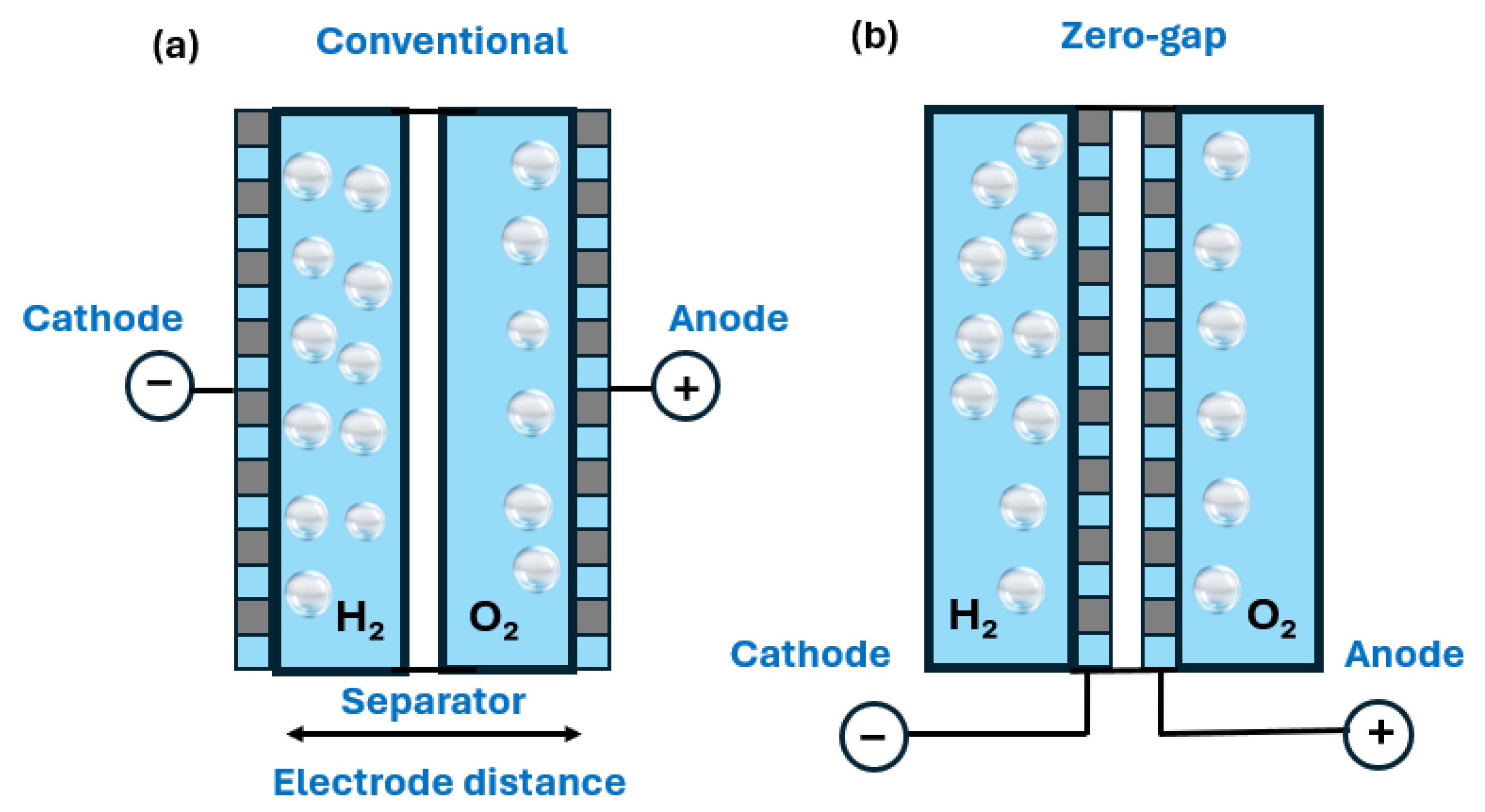
The experimental setup employed a zero-gap configuration (Figure 2), meaning that the space between the two electrodes was occupied only by the separator. This design prevents the recombination of the reaction products—oxygen (O₂) and hydrogen (H₂)—thereby reducing the risk of short circuits and facilitating the transport of hydroxide ions (OH⁻) [14]. Moreover, the zero-gap arrangement minimizes ohmic resistance compared to conventional configurations. In traditional systems, where the electrodes are positioned at opposite ends of the electrochemical cell, the increased distance between them leads to higher resistance and lower efficiency. Such setups also require the use of porous electrodes to promote electrolyte–membrane interaction and to enable hydroxide ion as previously described [8].

The choice of electrolyte is also crucial, as it governs ion transport within the electrochemical cell. Ionic conductivity directly affects the mobility of charged species—particularly at the cathode and anode—thereby influencing the efficiency of the half-reactions.

Aqueous solutions of potassium hydroxide (KOH) and sodium hydroxide (NaOH) are commonly used because of their high ionic conductivity. In this study, a 30 wt% KOH solution was selected, as it offers the highest ionic conductivity under standard conditions and provides excellent corrosion resistance [15,16].

To enhance the efficiency of electrolysis and hydrogen production, bubble accumulation on the electrode surfaces was addressed. A high bubble density creates a physical barrier between the electrolyte and electrodes, hindering the chemical reaction [17]. This accumulation obstructs electron transfer, increases the electrolyte resistance, raises the cell voltage, and decreases electrochemical efficiency. To mitigate this effect, piezoelectric actuators were used to generate ultrasound vibrations, detaching bubbles from the electrode surfaces and reducing their size. This approach minimizes bubble coalescence, increases the active electrode area, and improves the electron exchange in the electrolyte [18]. Consequently, the decongestion of the electrodes lowers electrical resistance, reduces cell voltage, and enhances efficiency.

The study then focused on the numerical analysis of high-speed video recordings of the electrolysis process to isolate the different entities within each frame. Previous works have employed various methods for this purpose. Some applied sequential digital filters—such as a median filtering followed by Otsu thresholding [19]—while others used the Hough transformation [20], a technique that detects geometric shapes by correlating points in an image. Although effective under simple conditions, its performance decreases when bubbles overlap.

The challenge becomes more pronounced due to the image artifacts (e.g., electrode pores misidentified as bubbles [21] and higher current densities, which produce denser and more chaotic bubble formation [22]. In this context, machine learning emerged as a powerful tool for interpreting experimental video data. Trained on annotated datasets, these models can identify complex objects with high accuracy. Their effectiveness depends on the chosen architecture. For instance, some studies have used the StarDist model, which represents objects by radial lines extending from their centers to their boundaries, assigning probabilities to determine object presence [22].

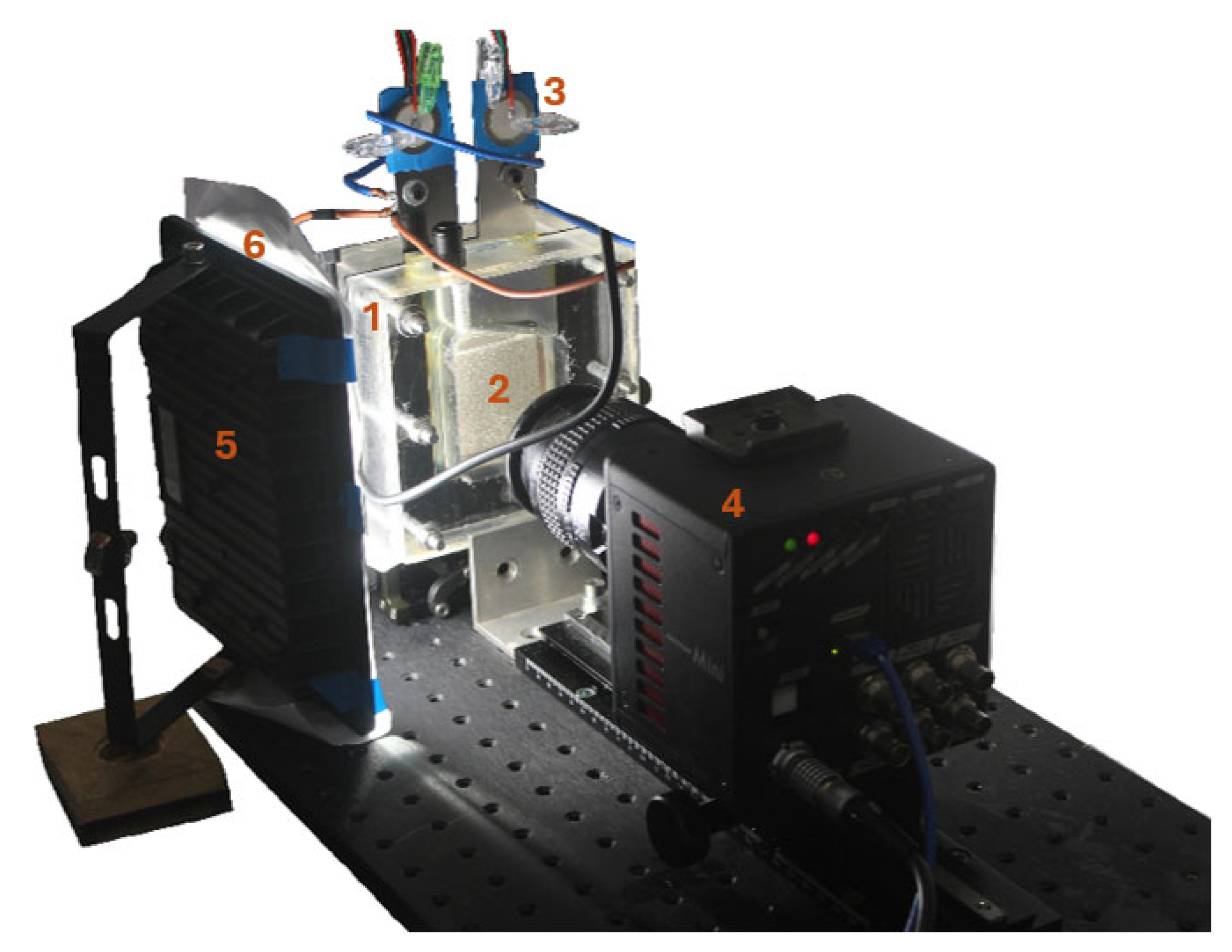
The electrochemical cell consisted of two porous nickels electrodes: each 2 mm thick. The pores acted as nucleation sites for bubble formation at different depths, thereby increasing the number of active sites for gas generation. Ideally, the bubble diameter corresponds to the pore size, enabling better control of bubble dimensions. The electrodes were immersed in the electrolyte solution to promote ion migration toward their surfaces. Figure 3 shows a general view of the experimental setup and the electrochemical cell.

To ensure efficient electron transport from the power source to the electrodes, each nickel electrode was connected to a conductive material. A diaphragm was placed between the two electrodes to divide the cell into two chambers, allowing hydrogen to form in one chamber while still permitting the passage of hydroxide ions (OH⁻) between compartments. Figure 4 presents an exploded view of the electrochemical cell.

Additionally, a rubber diaphragm was placed on each electrode to ensure watertight separation of the chambers, effectively preventing gas or liquid leakage that could compromise the experiment’s integrity. The setup was meticulously designed with sampling ports for collecting the electrolysis products. Transparent windows on the outer surfaces of both electrodes provided visual access while maintaining hermetic sealing of the cell.

The image acquisition and subsequent analysis were performed after the electrolytic system reached a quasi-steady operating regime. Initial transient stages, characterized by unstable bubble nucleation and electrode wetting effects, were intentionally excluded to ensure that the analyzed images represented statistically stable bubble dynamics.

4. Experimental Protocol

4.1. Electrolysis Observation

To observe the electrolysis reaction at the cathode, a high-speed camera was mounted on a rail facing the cathode window within the experimental setup, as shown in Figure 5.

A slim light projector was used to optimize illumination, ensuring high-quality recordings and clear visualization of bubble formation. The electrochemical cell consisted of:

• Two porous nickel electrodes.
• A potassium hydroxide (KOH) electrolyte.
• A current generator.
• A voltmeter measuring the potential difference between electrodes and a second voltmeter measuring the voltage across a cable, allowing precise calculation of current intensity through using Ohm’s law.
• A high-speed camera connected to a PC for image acquisition.

The experiments were initially conducted without ultrasound vibrations to avoid collateral effects such as electrolyte heating and interference from residual bubbles. Due to electrode porosity, bubbles formed throughout the electrode thickness. When the current was interrupted, some bubbles remained trapped within the structure, potentially distorting subsequent measurements. To prevent this, the protocol included mechanical percussion of the electrode surface before each test, dislodging trapped bubbles. A short waiting period was observed after setting up a new current to allow the system to reach a steady-state bubble dynamics regime.

The experimental procedure involved the following steps:

• Percuss the electrode surface to release residual bubbles from previous tests.
• Set the current intensity to the desired value.
• Wait two minutes to allow stabilization.
• Record the cathode region using the high-speed camera.

The protocol was repeated for each change in current intensity. A second phase of experiments was conducted with piezoelectric actuators activated to introduce controlled vibrations at the electrode surface. A total of 10 videos were collected, comprising 1504 frames. Tests were performed with and without ultrasonic actuation at current intensities of 0.040, 0.070, 0.130, 0.190, and 0.250 A. Measurements below 0.040 A were deemed ineffective, as the corresponding voltage (1.645 V) barely exceeds the theoretical minimum of 1.48 V required to initiate electrolysis. This threshold also considers the overpotential caused by electrolyte resistance.

4.2. Manual Determination of Bubbles Characteristics

The segmentation masks used for training and validation were generated through manual annotation of the high-speed images. Bubble boundaries were traced using a combination of polygonal contouring and pixel-level refinement to ensure accurate delineation of both large and small bubbles. All annotations were performed by a single trained annotator to maintain consistency across the dataset. While this approach minimizes stylistic variation in the masks, it does not allow for a direct assessment of inter-annotator variability. This represents a limitation of the present study, as differences in annotation style can influence the ground-truth labels used for training deep learning models. Future work should incorporate multiple annotators and quantify inter-annotator agreement—using metrics such as the Dice coefficient or intersection-over-union—to better characterize annotation uncertainty and its impact on segmentation performance.

5. Numerical Methods

A dedicated tool was developed to streamline result extraction at the end of each experiment, accelerating data processing while maintaining high reliability. The raw data consisted of high-speed video recordings capturing hydrogen bubble formation and rise at the cathode. Each frame contained approximately 40 bubbles, and with around 1500 frames per video, the data volume was substantial. Recordings were obtained under varying conditions, with and without piezoelectric actuation, across five current intensities.

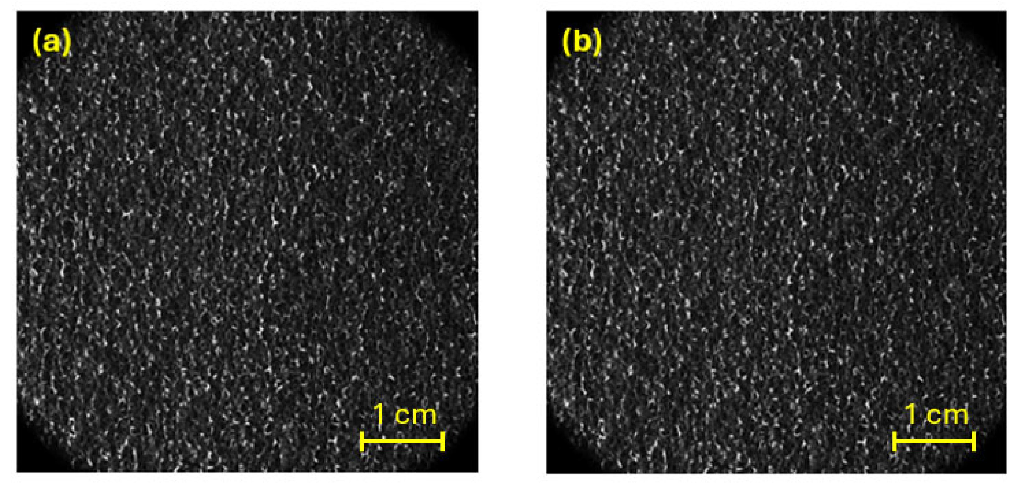
Given the dataset scale, an automated analysis was essential. The main objective was to isolate bubbles from the background using image segmentation, a computational technique that divides an image into pixel groups with distinct characteristics. Before segmentation, however, a pre-processing step was necessary. The images were grayscale (pixel values 0–2550), which allowed bubble identification and extraction from the porous nickel electrode, as illustrated in Figure 6.

A pre-processing step was required to remove the porous electrode pattern from the background, as interfered with bubble recognition. Without correction, electrode structures could be misinterpreted as bubbles, reductions algorithmic accuracy.

5.1. Image Pre-Treatment

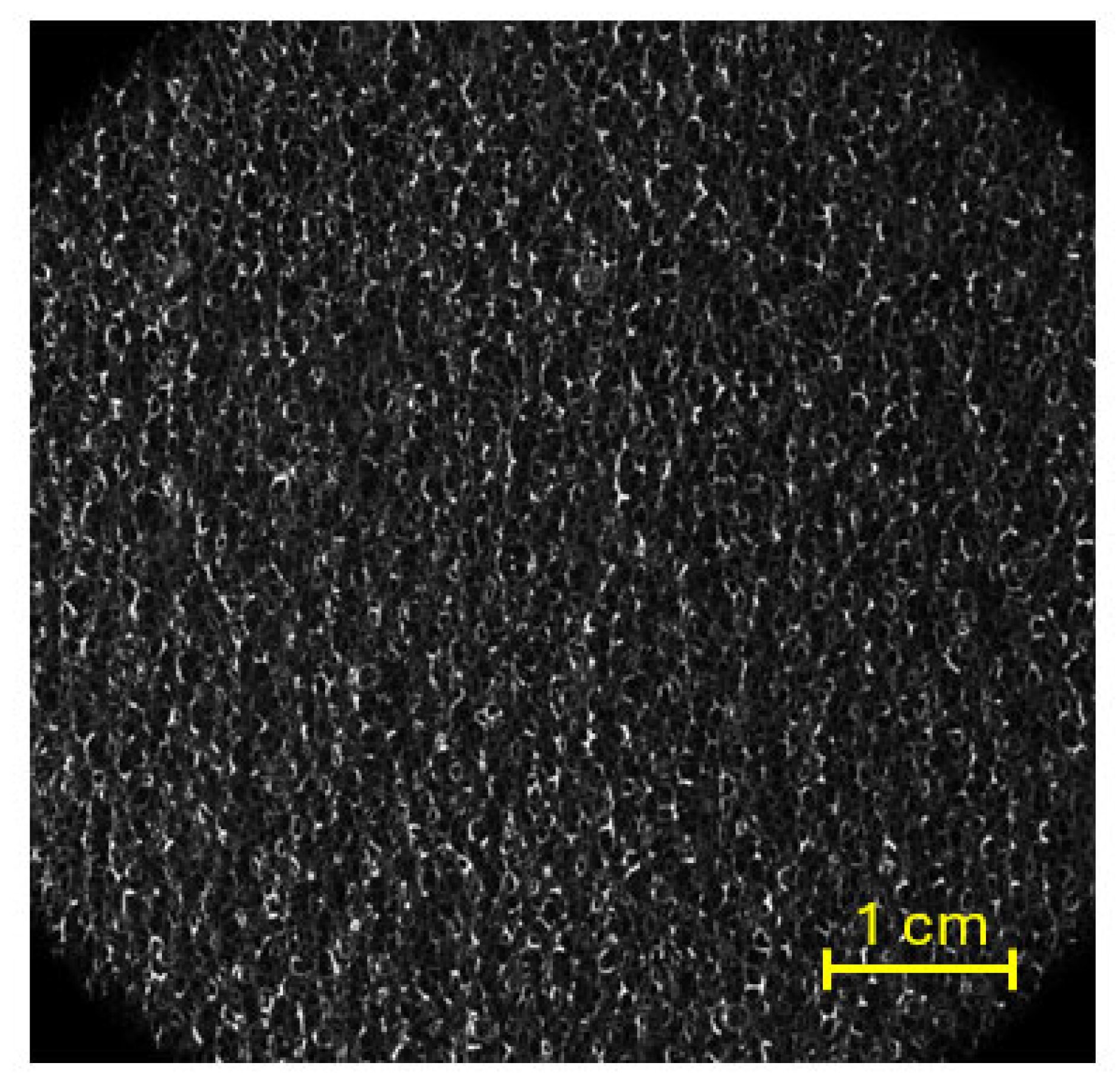
To eliminate the background, a pixel-wise averaging method was applied to a sample of frames. Due to the high bubble density, the electrode was obscured in many areas. Thus, averaging pixel intensities across a sufficient frame sample reconstructed the static background (mainly the electrode surface), as shown in Figure 7.

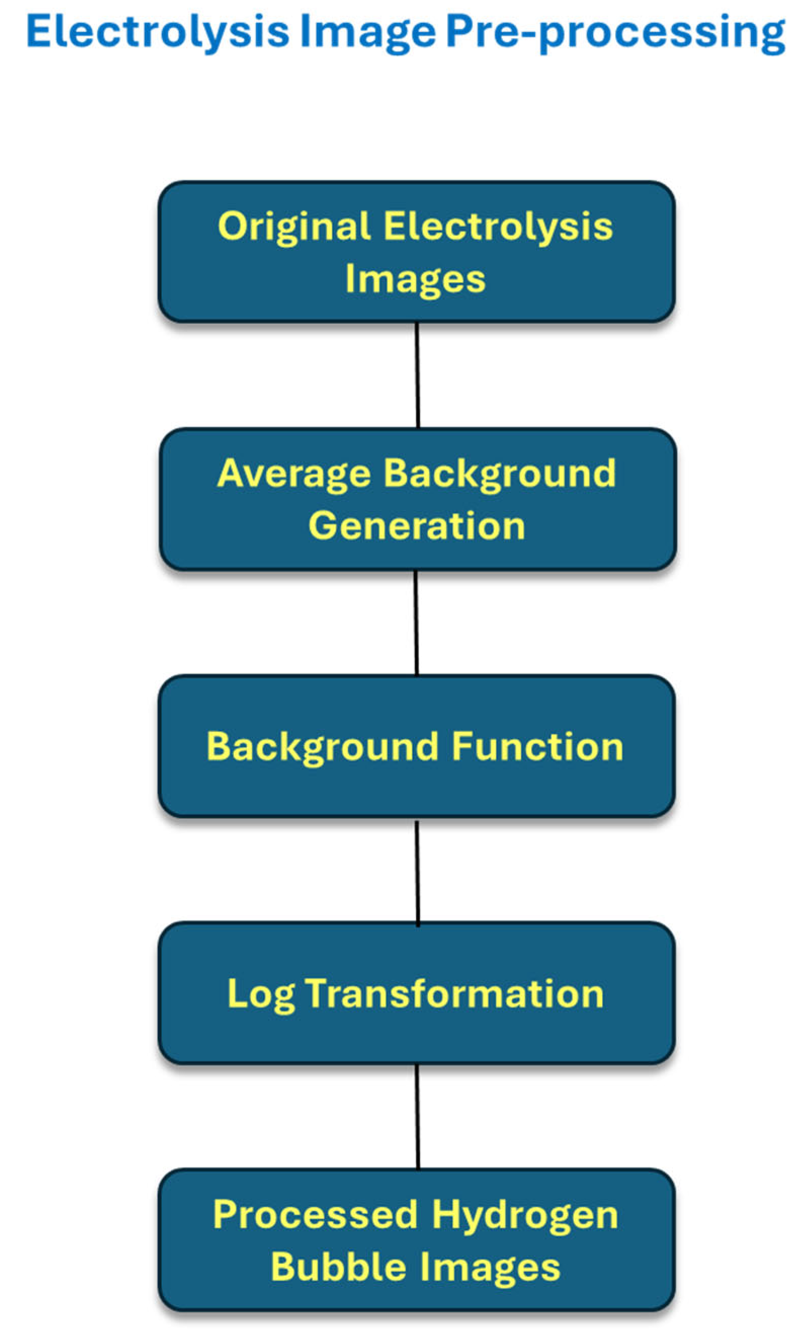
In the background, stationary bubbles adhered to the electrode were also visible. To remove them, a background subtraction technique was applied using a mean image computed from 30 frames before and 30 after each target frame, accurately representing static features. This mean image was subtracted from each frame, producing background-free images. To enhance contrast, a logarithmic transformation was then applied, improving bubble visibility (Figure 8).

This process improved bubble detection accuracy by removing static elements. The pre-processing steps were:

• Reference window selection: 30 frames before and after each target frame were chosen.
• Mean image calculation: the pixel-wise average generated a static background.
• Background subtraction: isolating moving hydrogen bubbles.
• Logarithmic transformation: enhancing contrast for better contour detection.

The result was a clean sequence of images suitable for reliable dynamic bubble identification. The main pre-processing steps are summarized in Figure 9.

Background subtraction was employed to isolate bubble contours; however, this approach can introduce non-negligible artifacts when applied to porous electrodes. The complex microstructure of materials such as nickel foam or sintered metal causes depth-dependent light scattering and local intensity fluctuations that are not temporally stable. As a result, the “background” is not truly static, and the subtraction process may amplify these variations, producing false edges, flickering features within pores, or apparent microbubbles that do not correspond to actual gas evolution. These artifacts can bias the quantitative extraction of bubble size, nucleation density, and detachment frequency, particularly for small or partially occluded bubbles. Although the overall trends reported in this work remain robust, the potential influence of electrode porosity on segmentation accuracy should be acknowledged. Future studies may benefit from adaptive background modeling, temporal averaging, or machine learning-based segmentation methods to mitigate these effects.

5.2. Ilastik Software

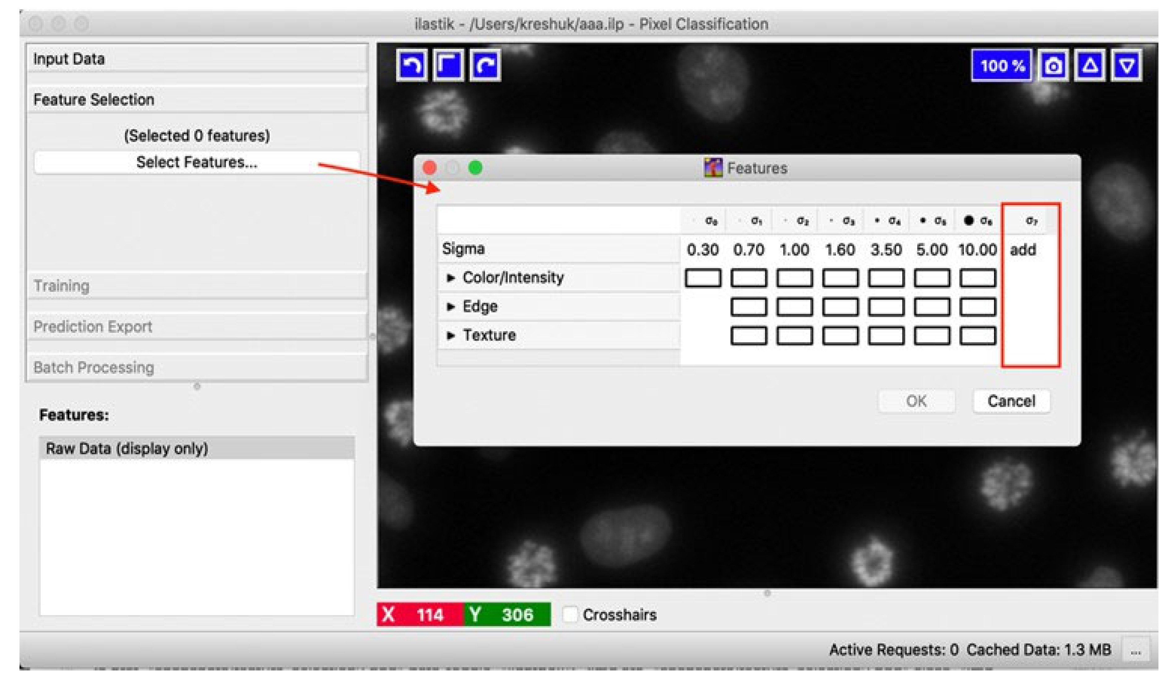
The first segmentation method used was Ilastik, v. 1.4.1.post1 an open-source tool for pixel-level classification and segmentation. Developed by the Heidelberg Collaboratory for Image Processing (Heidelberg University, 2011), Ilastik allows users to define categories that the algorithm learns to recognize. Classification relies on feature selection (intensity, texture, edges), implemented through Gaussian-based filters, where the sigma parameter determines the level of smoothing (Figure 10) [22].

A linear numerical filter was applied by multiplying the image illuminance E by a kernel filter A in the frequency domain, followed by convolution in the spatial domain [23]:

$${\mathrm{E}}_{\mathrm{f}\mathrm{i}\mathrm{l}\mathrm{t}\mathrm{e}\mathrm{r}}=\mathrm{A}\left(\mathrm{h},\mathrm{k}\right)·\mathrm{E}\left(\mathrm{i},\mathrm{j}\right)={\sum }_{\mathrm{h}=-\mathrm{m}/2}^{\mathrm{m}/2}{\sum }_{\mathrm{k}=-\mathrm{m}/2}^{\mathrm{m}/2}\mathrm{A}(\mathrm{h},\mathrm{k})·\mathrm{E}(\mathrm{i}-\mathrm{h},\mathrm{j}-\mathrm{k})$$

(5)

For a Gaussian filter, the kernel A is derived from the Gaussian function:

$$\mathrm{A}(\mathrm{h},\mathrm{k})={\displaystyle \frac{1}{2\pi {\sigma }^2}}\cdot {\mathrm{e}}^{-{\displaystyle \frac{{\mathrm{h}}^2+{\mathrm{k}}^2}{2{\sigma }^2}}}$$

(6)

The kernel coefficients were normalized so that their sum equaled one, preserving image brightness. The Gaussian filter reduces noise while retaining key details. A smaller $\sigma$ enhances fine details, while a larger $\sigma$ smooths the image.

This choice had a significant impact on the training process of the model. Notably, Ilastik includes an automated feature selection tool that helps optimize both the feature types and their corresponding values. The choice of features also affects training time, as more complex configurations may require longer processing. The next stage involved using a set of pre-processed images acquired from the electrolysis experiments. In this step, each object within the image was manually labeled as either Background or Bubble, depending on its nature. The labels enabled the model to learn and recognize relevant characteristics in the training images—particularly those influenced by Gaussian filters with distinct parameters. Figure 11 shows a representative labeled image obtained at 0.250 A (silent condition).

In this study, 24 images were manually labeled, selected from different acquisitions covering multiple current intensities, both with and without ultrasound. This diversity ensured that the training dataset adequately represented the range of expected operating conditions. The goal was to build a model capable of providing accurate predictions even when input images varied in bubble size, density, and quality. Although this diversity inevitably increased training time the number of images required for reliable predictions, it was deemed essential for enhancing the model’s generalization ability.

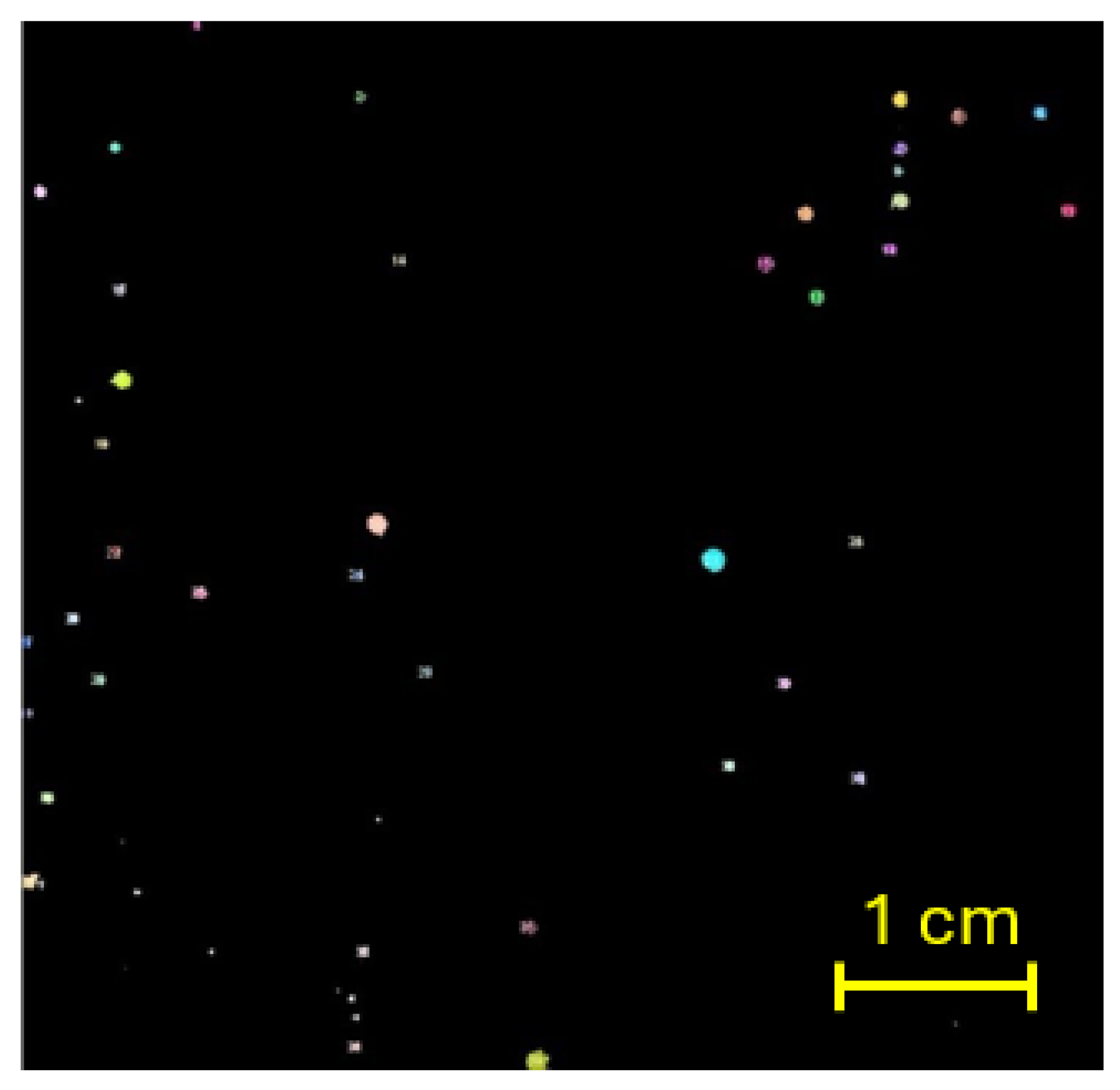
The model was trained using the Ilastik software, which relies on a Random Forest algorithm [22,24]—a machine learning method based on an ensemble of decision trees. Each tree evaluates a random subset of input features and makes classification decisions through a hierarchy of conditions. These decision points, or nodes, test variables such as pixel intensity, texture, and other image characteristics. During training, the model learned the optimal conditions for classifying each pixel as either “Background” or “Bubble.” Once trained on the 24 labeled images, the model was applied to new inputs to predict the class of each pixel. The resulting prediction outputs were saved in HDF5 format, which stores both the segmented image and the associated probability maps. For visualization, these files were converted into more accessible formats such as .PNG. Figure 12 illustrates the prediction result generated by the Ilastik model for frame 100, corresponding to an experiment at 0.190 A without ultrasound activation.

In the output image generated by the Ilastik model, the segmented entities appeared in white against a black background. The segmentation process classified pixels into bubbles (white) and background (black).

5.3. U-Net Model

Ilastik was initially chosen for its user-friendly interface, providing an intuitive approach to image classification [22]. Nevertheless, the need for a more autonomous and flexible solution emerged—particularly due to the HDF5 output format of Ilastik, which requires additional post-processing. This led to a shift in the focus toward models that could be implemented directly within a Python environment, allowing greater control and integration. Among the alternatives, the U-Net architecture was selected. U-Net is a Convolutional Neural Network (CNN) originally developed for biomedical image segmentation at the Department of Computer Science, University of Freiburg, Germany. CNNs are inspired by the structure of the human nervous system, consisting of multiple layers organized into blocks that progressively extract and learn features from the input data [25].

The U-Net model derives its name from its U-shaped architecture, which comprises a series of contracting paths followed by expanding paths. The contracting paths capture contextual information and extract deep features, while the expanding paths enable precise localization and refinement of those features [26]. In this study, the functioning of the learning model used to enhance and train the U-Net architecture is detailed below.

It is important to note that the U-Net model was trained on a limited dataset of 24 manually annotated images. This number was intentionally restricted due to the high annotation cost associated with high-resolution experimental images. Therefore, the U-Net implementation in this work should be interpreted as a proof-of-concept, aimed at evaluating feasibility rather than achieving full generalization. To mitigate dataset size limitations, data augmentation techniques were applied during training including rotations, flips, contrast adjustments, and synthetic noise, effectively increasing the diversity of the training samples. While these strategies improve the stability of the model, the limited dataset size remains a constraint and may impact on the segmentation accuracy, particularly for small or partially occluded bubbles. Future work should incorporate larger datasets, automated annotation pipelines, or transfer learning approaches using pre-trained segmentation networks to further enhance the performance of the model.

5.3.1. Encoding

The U-Net model begins with an encoding phase that processes the input image. For grayscale images, the input contains a single channel, whereas colored images have three. The encoding phase applies two successive convolutional layers, followed by a ReLU activation function and a max pooling operation. Each image is represented as a two-dimensional array, where each element corresponds to a pixel value. In grayscale images, pixel values range from 0 (black) to 255 (white). The convolutional layers use small filters—typically of size 3 × 3—to capture local patterns within the image. After each max pooling operation, the number of features maps doubles, allowing the model to analyze increasingly complex and detailed structures. The sequence of convolution, ReLU activation, and max pooling was repeated three times to gradually extract higher-level features. A convolutional layer performs the convolution operation between the input image and a filter.

The filter—a 3 × 3 matrix—slides across the image with a defined stride. At each position, the element-wise product between the filter and the corresponding image patch is computed, summed, and normalized by the number of pixels involved. This operation produces a new matrix that highlights the presence of specific features in the image. These filters, or kernels, are learned during training and designed to detect meaningful structures from the input data. The resulting feature maps indicate how strongly different regions of the image corresponded to the learned patterns. After convolution, the Rectified Linear Unit (ReLU) activation function is applied, defined by Equation (7):

$$\mathrm{f}\left(\mathrm{x}\right)=\mathrm{m}\mathrm{a}\mathrm{x}(0,\mathrm{x}) \mathrm{for} \mathrm{all} \mathrm{real} \mathrm{values} \mathrm{x}$$

(7)

This function sets all negative input values to zero, preventing issues such as vanishing gradients—where values converge toward zero—and exploding gradients, where they diverge toward infinity [25].

Subsequently, the model performs a max pooling operation, which reduces the image by converting it into a smaller matrix. This is done by sliding a 2 × 2 window across the image with a predefined stride and retaining only the maximum value within each window. This technique helps reduce computational complexity while preserving the most significant features.

After the max pooling, the image dimensions are reduced by half, effectively compressing the data while retaining the most relevant features. As a result, computational load decreases, but the essential information for further analysis is preserved.

5.3.2. Decoding

This stage follows the encoding phase and does not include any further max pooling operations. At this point, the image has been reduced to 128 × 128 pixels and represented by 256 feature channels, derived from an initial input size of 512 × 512. The decoding phase restores the spatial information lost during the encoding and gradually reduces the number of features to reconstruct the original image. This is achieved through deconvolution (transposed convolution) operations, which increase the spatial resolution of the feature maps. Afterward, a copy-and-crop operation is performed: feature maps from the corresponding encoding layer are copied and merged with those from the decoding layer. This fusion is achieved via concatenation along the first tensor dimension, effectively combining the features from both phases. This process recovers the spatial details lost during max pooling in the encoding phase. The final decoding step applies a 1 × 1 convolution filter, which projects the feature vector of each pixel into a probability value representing its likelihood of belonging to a given class. In this binary segmentation task, the output is a single-channel feature map representing the probability of each pixel being classified as “Bubble.” A probability map is generated, and binary segmentation is performed by applying a threshold (p = 0.5 in this case) to determine the final pixel classification.

5.3.3. U-Net Implementation

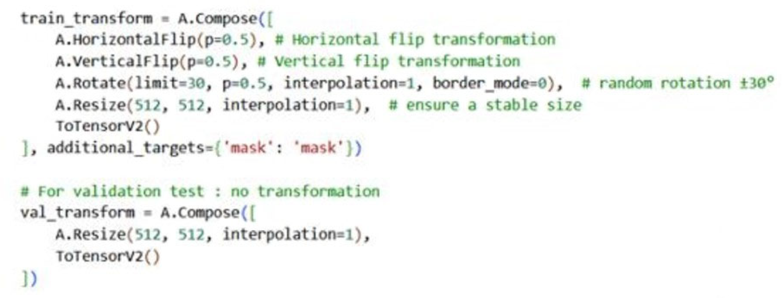
The next step was to implement the model using Python script. For this purpose, Google Colab was used, providing free access to a GPU with 12 GB of memory—an essential resource, as computational limitations would otherwise represent a significant constraint for this study. The implementation relied on the PyTorch library, which offers a wide range of pre-defined objects and functions that simplify the construction of the U-Net model. In addition, the Albumentations library was employed to handle data augmentation, a technique that enhances model training by generating new variations in existing images without increasing the actual dataset size. This was achieved through transformations such as vertical and horizontal flips and rotations, which simulate new visual scenarios for the model. As a result, it was possible to increase the number of training epochs, that is, the number of times each image is processed by the model. In this context, the variable p (Figure 13) represents the probability that a transformation will be applied to an image. The variable interpolation = 1 (Figure 13) ensures that both the image and its corresponding mask undergo the same transformation, maintaining alignment between them.

The training images were first resized to 512 × 512 pixels to match the defined hyperparameters. After resizing, both the image and its mask were converted into PyTorch tensors, which serve as the foundation for subsequent operations. For validation, the val_transform variable was defined. Since data augmentation was unnecessary during validation, the images were simply resized and converted into tensors for testing.

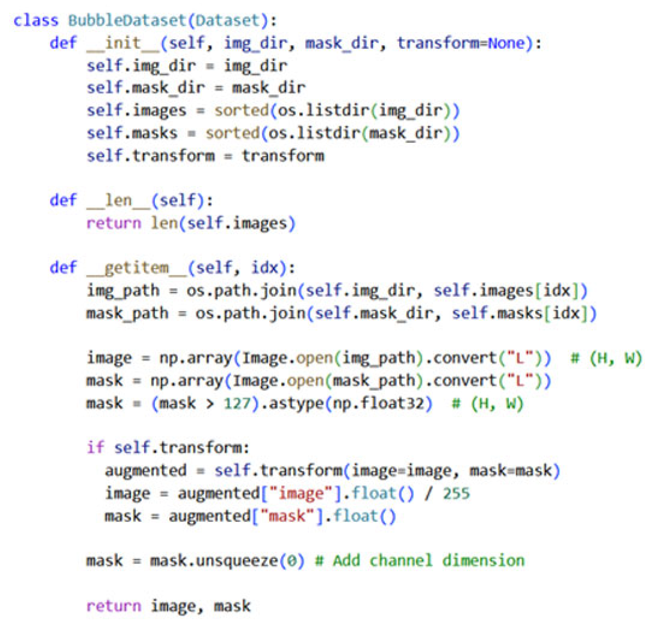
Apart from data augmentation, a customized class named BubbleDataset (Figure 14) was created. This class incorporated several functions to facilitate the import of image data into the Python environment. It handled both the raw training images and their corresponding masks, forming the dataset on which the model was trained. The __init__() function stored the relevant objects within the class instance, including the images, masks, file paths, and transformation settings. The __len__() method returned the total number of images available in the dataset. Finally, the __getitem__() method assigned a path to each image, opened it using the Image.open function from the PIL library, and converted it to grayscale using .convert(‘L’).

This operation was performed simultaneously on both the image and its corresponding mask. The mask was first binarized and then converted to 32-bit floating point format (float32) to ensure compatibility with the expected input type for transformation functions. Subsequently, identical transformations were applied to both the image and the mask to enable data augmentation, using the defined augmentation parameters.

Afterward, the image was converted into a floating-point format and normalized. The mask was also converted to float, and a channel dimension was added using the squeeze() function to match the expected input structure.

In PyTorch, each image is represented as a tensor with three dimensions:

$$(\mathrm{C},\mathrm{H},\mathrm{W})$$

where

• C is the number of channels corresponding to extracted features;
• H is the height (rows);
• W is the width (columns).

This tensor format supports image manipulation throughout the various stages of the model, particularly within the U-Net architecture, which relies on these feature channels for segmentation tasks.

5.3.4. Implementation of Convolutional Layers and U-Net Architecture in PyTorch

The first step in building the model involved implementing the convolutional layer using the conv_block() function., This function replicated a sequence of operations in which each block performed two consecutive 2D convolutions, each followed by a ReLU activation. This pattern ensured non-linearity and feature extraction at each stage. In all convolutional layers, a padding of one was applied. Padding is a technique used to preserve the spatial dimensions of the input matrix during convolution. Specifically, a padding value of one means that one row and one column of zeros were added around the input matrix, allowing convolution to be applied without reducing the output size.

After that, the U-Net class was defined, inheriting from nn.Module of PyTorch, which is the base class for all neural network models in PyTorch. Within this class, model parameters and layer definitions were initialized, and the forward() method was implemented to define the data flow through the network. The architecture followed the classic U-Net structure, consisting of an encoding path (a series of convolutional operations followed by max pooling) that progressively reduced spatial dimensions while increasing feature depth. The bottleneck, located at the deepest layer of the network, marked the transition between encoding and decoding. The decoding path involved upsampling (typically via transposed convolutions) and concatenation of the upsampled features with corresponding features from the encoding path. These skip connections help retain spatial information lost during the downsampling. This design enabled the model to learn both global context and fine-grained details, making it particularly effective for image segmentation.

In this work, the model architecture involved successive encoding operations—convolutional followed by max pooling—leading to the bottleneck, the transitional point between encoding and decoding. The decoding phase incorporated deconvolution operations, which were combined with their symmetric counterparts from the encoding path through concatenation along dimension one of the tensor (the channel axis). This allowed the model to merge fine-grained spatial details from the encoder with contextual information from the decoder.

The final convolutional layer produced an output with a single channel, representing a probability map. Its purpose was to project the learned feature maps into class probabilities, which explains the use of a single output channel. Unlike the initial U-Net model described in Figure 15, the current architecture avoided further spatial reduction during convolution. Consequently, there was no need for spatial reconstruction after deconvolution, as illustrated in Figure 15. Instead of reconstructing, the image, the decoding phase focused on contextual enrichment, aligning with the U-Net structure by merging feature dimensions rather than spatial ones.

5.3.5. Model Training Workflow in PyTorch

Once the model operations were implemented and its structure defined—specifying how data flowed through it, the next step was to train the model so it could refine its internal parameters (weights). It is important to note that refining the weights did not immediately guarantee high accuracy, as the model must learn through repeated exposure to the training data. Training involved adjusting the model weights epochs, where each epoch represents one complete pass through the training dataset. In convolutional neural networks, these weights correspond to the kernels (or filters) used in the convolutional layers.

To initiate training, the input image and its corresponding mask (label) were transferred to the designated device—a Google Colab NVIDIA T4 GPU—which enabled faster and more efficient computation compared to a CPU. The model processed the input tensor using PyTorch, generating predictions. Before computing the loss, the optimizer gradients were reset using optimizer.zero_grad() to prevent accumulation from previous iterations. The loss function compared the predicted output with the ground truth mask. Here, the nn.BCEWithLogitsLoss() function from PyTorch was used, suitable for binary classification tasks. The function calculates the error between the predicted and the actual values and aims to minimize it. In the setup of this work, it was used reduction = ‘mean’, averaging the loss across all pixels. The loss function can be expressed by Equation (8):

$$\mathrm{l}\mathrm{o}\mathrm{s}\mathrm{s}={\displaystyle \frac{1}{\mathrm{N}}}{\sum }_{\mathrm{n}=1}^{\mathrm{N}}{\mathrm{w}}_{\mathrm{n}}·\mathrm{B}\mathrm{C}\mathrm{E}\left({\mathrm{y}}_{\mathrm{n}},{\mathrm{x}}_{\mathrm{n}}\right)$$

(8)

where y_n are the predicted values, x_n are the ground truth masks, and w_n are optional pixel weights.

To optimize the model (Figure 16), loss.backward() computed the gradients of the loss function with respect to each weight. Then, optimizer.step() updated the weights based on these gradients, moving them in the direction that minimized the loss. This iterative process continued across epochs, gradually improving model performance.

After completing all training interactions, the model’s performance was evaluated using an unseen image outside the training set. Before this step, the key hyperparameters were defined, including batch size, number of epochs, image dimensions, and learning rate. During training, the model grouped individual images into batches of size N, optimizing memory usage and accelerating GPU processing. In this study, a batch size of 4 was selected due to the limited dataset size.

The number of epochs—defined as the number of times the model processes each image—was another critical factor. Multiple passes are typically required to obtain meaningful learning, but excessive epochs can cause overfitting, where the model becomes overly specialized in the training data. To mitigate this, data augmentation techniques (vertical/horizontal translations and rotations up to five degrees) were applied, allowing the model to perceive the same image in varied configurations.

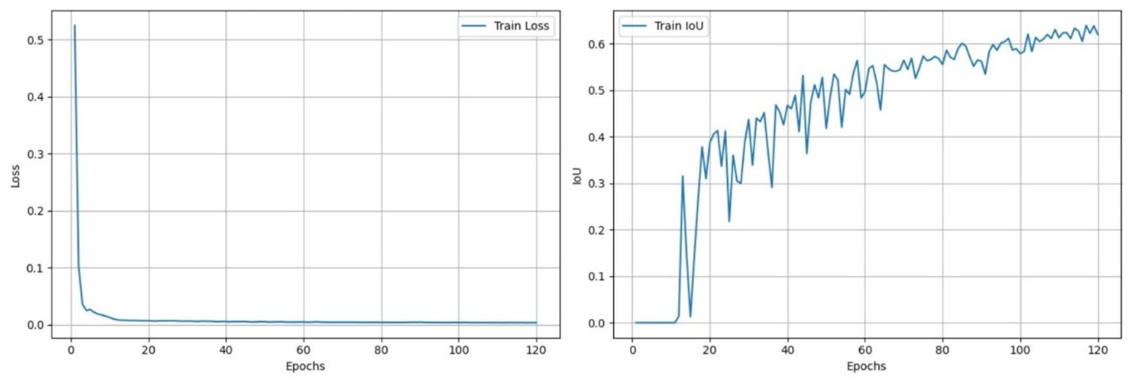
An empirical study was conducted to analyze the evolution of the Intersection over Union (IoU) metric relative to the number of epochs. IoU is defined as the ratio between the area of overlap (intersection) and the combined area (union) of the predicted object and its corresponding ground truth mask. A higher IoU indicates more accurate segmentation.

Conversely, a low IoU value reflects poor prediction accuracy, with minimal overlap and a larger union, causing the metric to approach zero. The results of this analysis are presented in Figure 17, which illustrates the evolution of both the loss function and the IoU metric as functions of the number of epochs during the training of the U-Net model, using data augmentation on a dataset of 24 images with a batch size of 4.

The loss function showed a significant decrease during training, reaching a plateau around 17 epochs. In parallel, the IoU metric steadily improved, peaking at near 120 epochs. However, further training was constrained by GPU resource limitations, restricting the number of epochs. Although the original images had a resolution of 1024 × 1024 pixels, processing such high-resolution data was computationally intensive and led to excessive GPU memory usage. Therefore, the images were downscaled to 512 × 512 pixels as a compromise between computational efficiency and spatial accuracy. This resolution reduction may introduce boundary inaccuracies, particularly for small bubbles close to the optical resolution limit. However, a qualitative inspection indicated that the larger bubbles remained well defined. The learning rate, which determines how frequently the model updates its weights, was set to 10⁻³. Once the model was fully trained, it was tested on an unseen image to assess the prediction quality. Future work may benefit from resolution-preserving architectures or patch-based training strategies to avoid the need for global image reduction. Figure 18 shows the prediction obtained using the PyTorch model.

The prediction results from the trained U-Net model revealed a binary segmentation that distinguished two classes: bubbles (white) and background (black). The model was trained using the provided dataset, repeatedly executing encoding and decoding operations while adjusting its weight based on the loss function to improve segmentation accuracy.

5.4. Fiji Software

Fiji v. 2.16.0 is an extended version of ImageJ, v. 1.54p an open-source image processing software developed at the Laboratory for Optical and Computational Instrumentation of the University of Wisconsin–Madison. The software supports traditional image processing operations such as thresholding and filtering and provides a broad range of plug-ins for advanced image analysis. In this study, Fiji was used to convert images into the HDF5 format—compatible with Ilastik—and to measure bubble dimensions using the Analyze Particles module. The TrackMate plug-in was employed for tracking operations, enabling bubble counting and determination of their release frequency.

Initially, a thresholding operation was applied to the grayscale predictions generated by the Ilastik model. Thresholding converts a grayscale image into a binary one by applying a defined threshold value m: pixels with intensity below m are set to zero, and those above m to one. This binary image allowed bubble counting and size distribution analysis and served as input for TrackMate to perform tracking across video frames.

Figure 19 presents a screenshot of the Analyze Particles module of Fiji, which identifies and isolates the bubbles in the image. Each bubble was assigned a unique ID, and its dimensions were measured using Fiji’s built-in analysis tools. The resulting data was exported as a .csv file for further processing.

Configuration and Operation of the TrackMate Plug-In

To use the TrackMate plug-in, several configuration and preparation steps were required. The first stage involved selecting the detector type, which identifies the hydrogen bubbles to be tracked. Once configured, the detector processed all 1504 frames in the sample, identifying bubbles in each frame. The tracking process established continuity between particles as they moved across frames, according to a set of user-defined parameters. After testing several detector–tracker combinations, the Thresholding Detector combined with the LAP (Linear Assignment Problem) Tracker yielded the most consistent results. For validation, the number of bubbles detaching from the electrode during the observation interval was manually counted.

• Thresholding Detector

The Thresholding Detector identifies entities whose pixel intensity exceeds a predefined threshold. Since the images had already undergone thresholding during pre-processing, this detector was the most suitable for isolating bubble regions based on intensity.

• LAP Tracker

The LAP Tracker links particles across consecutive frames by minimizing a cost function that combines Euclidean distance (D) and penalties (P) associated with differences in object features such as area, circularity, and intensity:

$$\mathrm{Cost}={(\mathrm{D}·\mathrm{P})}^2$$

(9)

where D is the Euclidean distance between two particles, and P is defined as

$$p=3·W·{\displaystyle \frac{\left|f_1-f_2\right|}{f_1+f_2}}$$

(10)

where W represents the weights associated with the characteristics, f₁ and f₂ are the features of entities m and k, respectively represent the characteristics of the m entity.

The tracker also supports gap closing, which reconnects track segments when a particle temporarily disappears and reappears in subsequent frames. This process is governed by:

• The maximum number of frames allowed between disconnections;
• The maximum spatial distance within which segments can still be linked.

Through these operations, TrackMate assigns each particle a predecessor and a successor or leaves it unlinked if no suitable match is found-based on the same cost-minimization principle [27].

In practice, Fiji was used to import the sample as an image sequence (File → Import → Image Sequence) and set the image type to 16-bit to obtain a black-and-white representation. A threshold of 255 was applied (Image → Adjust → Threshold) to binarize the image, setting all pixel values below 255 to 0 and those equal to 255 to 1. Next, the image scale was defined as 25 pixels per millimeter (Analyze → Set scale) by entering 25 for Distance in Pixels, 1 for Known Distance, and mm for Unit of Length. Figure 20 shows the user interface of the TrackMate plugin. Once scaled, the sequence was ready for tracking. The TrackMate plug-in was opened (Plugins → Tracking → TrackMate). The Thresholding Detector was selected with a threshold value of 254, ensuring that only pixels equal to 255 (white) were considered as objects. By clicking Preview, correctly detected bubbles appeared with a purple contour. The LAP Tracker was then selected to manage gap closing, allowing the software to reconnect bubbles that disappeared and reappeared without counting them as new objects. Figure 20 shows the TrackMate user interface.

Finally, under the Display options window, Spots option was selected, and the results were exported to a .csv file by clicking Export to CSV, generating a document containing all relevant tracking data.

6. Determination of the Size of Hydrogen Bubbles

To perform a detailed analysis of the hydrogen bubble distributions generated during electrolysis, it was necessary to develop a tool to process the predictions obtained from both the Ilastik and U-Net models. In both cases, the objective was to handle the numerical data extracted from the Analyze Particles module in Fiji, which analyzed the segmented images and generated tabulated characteristics for each detected entity-such as area, perimeter, and Feret diameter. Assuming the bubbles to be perfectly circular, their diameter (d) was calculated from the measured area (A) using Equation (11):

$$d=2\cdot \sqrt{{\displaystyle \frac{A}{\pi }}}$$

(11)

where d is the bubble diameter and A is the measured area.

This approach was preferred over the Feret diameter—which measures the distance between two extreme points of the object—because it better reflects the manual measurement method applied to the video samples. To evaluate the prediction accuracy, the Root Mean Square Error (RMSE) was calculated between the manually measured bubble diameters and those predicted by the Ilastik model. The RMSE, based on rea-, perimeter-, or Feret-derived diameter estimates, was computed using Equation (12):

$$\mathrm{R}\mathrm{M}SE=\sqrt{{\displaystyle \frac{1}{N}}{\sum }_{i=1}^N{\left(y_i-{\widehat{y}}_i\right)}^2}$$

(12)

where

• y_i is the manually measured characteristic of the $\mathrm{i}$-th bubble;
• ${\widehat{\mathrm{y}}}_{\mathrm{i}}$ is the corresponding predicted characteristic;
• N is the total number of matched entities.

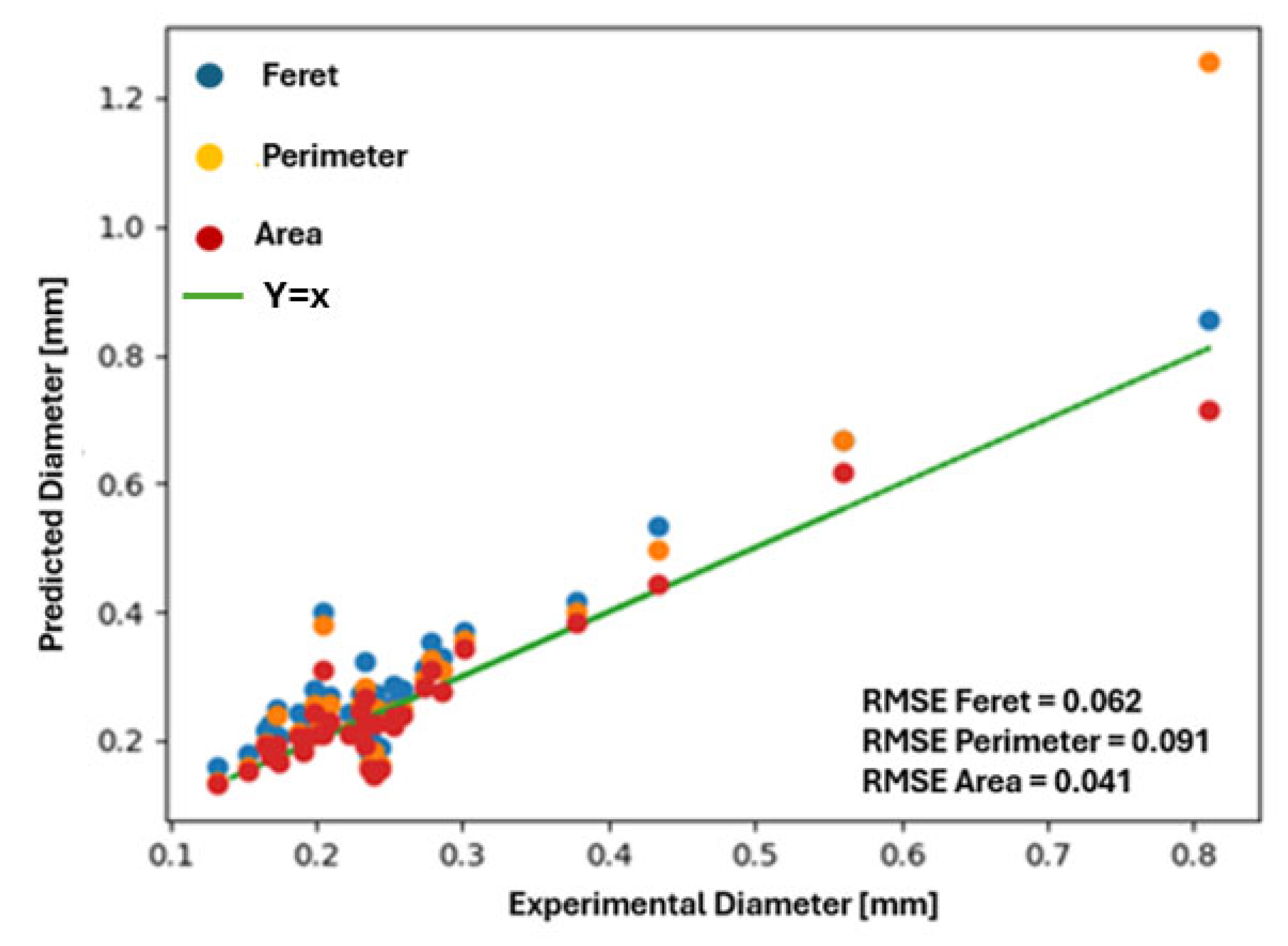
Figure 21 shows the measurement error of bubble diameters obtained through the different estimation methods.

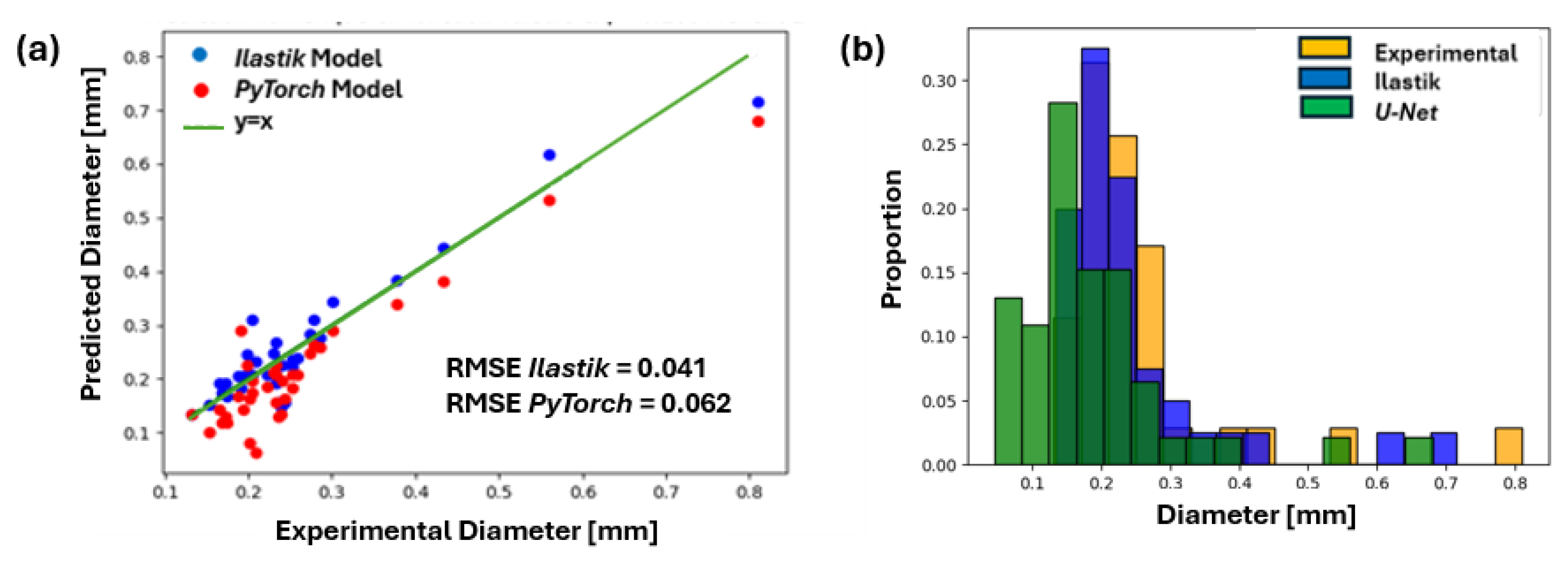
The RMSE is a reliable metric for assessing measurement accuracy, as it quantifies the average deviation of data points from the reference line y = x, where x represents experimental values. Expressed in millimeters, RMSE directly reflects the magnitude of the average error. To visualize and analyze the results from Fiji Analyze Particles module, a custom algorithm was developed in Python using the pandas library. The tool extracted and organized the tabulated data to evaluate the performance of each predictive model through graphical representation. In this plot, the x-axis corresponded to the manually measured bubble diameters, while the y-axis represented the predicted values. Two paired lists—one containing experimental measurements and another with model predictions—were constructed for one-to-one comparison. This approach allowed direct visualization of the bubble size distribution and facilitated the calculation of RMSE across all samples, quantifying the overall accuracy and reliability of both models.

7. Determination of the Bubble Release Frequency

The next step focuses on determining the hydrogen bubble release frequency from the electrode using an automated approach. This analysis relied on the previously developed U-Net model, which was used to predict the dimensions and occurrence of hydrogen bubbles. Although the Ilastik model was also evaluated, its implementation proved less efficient for processing large datasets, as each video recording contained 1504 frames, requiring an equal number of predictions. While Ilastik could handle these computations, it operated considerably slower than the U-Net model and required an additional step to convert the output files into HDF5 format. To streamline the workflow, the predictions generated by the U-Net model for each recording were directly processed in Fiji using the TrackMate plug-in. TrackMate produced a data table containing the identifier (ID) of each detected entity per frame, as well as a Track ID linking individual bubbles across consecutive frames—effectively recognizing each one as a single tracked object. A custom algorithm was then developed to extract the relevant tracking information from this dataset, enabling efficient analysis and accurate computation of the bubble release frequency.

8. Implementation of a Tracking Data Exploration Tool

The main objective was to quantify the number of hydrogen bubbles emerging from the electrode during the video recording. Using the tracking tool, a dataset was generated containing all detected bubbles, each identified by a unique Track ID. Visually, these bubbles appeared as they rose from the electrode within the video acquisition window.

To isolate only the bubbles that visibly emerged within the recorded frame, an algorithm was developed in Python using the pandas library to filter the tracking data and retain only the relevant trajectories. The filtering process consisted of the following steps:

• Initial calibration—Bubbles detected in the first two frames were excluded to initialize the counter at zero. This step accounted for potential detection errors and ensured that no bubbles were considered before actual formation began.
• Minimum duration filter—Tracks lasting fewer than 20 frames were removed. This filter eliminated transient noise and artifacts, such as background reflections or residual elements unrelated to bubble formation.
• Vertical displacement filter—Bubbles with a vertical displacement (difference between maximum and minimum y-coordinates) smaller than 0.5 mm were discarded. This condition removed false positives associated with static bright spots or imperfections on the porous electrode.
• Initial position filter—Bubbles whose first appearance occurred below the 18.2 mm mark on the vertical axis (measured from top to bottom) were excluded. This ensured that only bubbles originating within the visible region of the electrode were counted, preventing those entering the frame from being included.

After applying these filters, the remaining tracks corresponded to bubbles that genuinely emerged from the electrode surface. To determine the bubble release frequency, the total number of detected bubbles was divided by the area of the acquisition window. Considering a square acquisition window of approximately 20.5 mm per side and a recording time of 3 s, the bubble release frequency was calculated per unit surface area.

The adopted Python script implementing this procedure is shown below.

•               import pandas as pd
              

• # Load TrackMate output CSV
• # Replace 'trackmate_data.csv' with your actual filename
• df = pd.read_csv('trackmate_data.csv')
• # Assumed column names — adjust if needed
• # 'Track ID', 'Frame', 'Y', 'X' are typical columns from TrackMate
• # Ensure 'Y' is in millimeters or convert if needed
• # Step 1: Remove bubbles present in the first two frames
• first_two_frames = df[df['Frame'] <= 2]['Track ID'].unique()
• df_filtered = df[~df['Track ID'].isin(first_two_frames)]
• # Step 2: Remove bubbles tracked in fewer than 20 frames
• track_counts = df_filtered['Track ID'].value_counts()
• valid_tracks = track_counts[track_counts >= 20].index
• df_filtered = df_filtered[df_filtered['Track ID'].isin(valid_tracks)]
• # Step 3: Remove bubbles with vertical displacement < 0.5 mm
• vertical_displacement = df_filtered.groupby('Track ID')['Y'].agg(['min', 'max'])
• vertical_displacement['delta'] = vertical_displacement['max'] - vertical_displacement['min']
• valid_tracks = vertical_displacement[vertical_displacement['delta'] > 0.5].index
• df_filtered = df_filtered[df_filtered['Track ID'].isin(valid_tracks)]
• # Step 4: Remove bubbles whose first appearance is below 18.2 mm
• first_positions = df_filtered.groupby('Track ID').apply(lambda g: g[g['Frame'] == g['Frame'].min()])
• valid_tracks = first_positions[first_positions['Y'] <= 18.2]['Track ID'].unique()
• df_filtered = df_filtered[df_filtered['Track ID'].isin(valid_tracks)]
• # Final count of bubbles that emerged from the electrode
• bubble_count = df_filtered['Track ID'].nunique()
• # Calculate release frequency per surface unit
• acquisition_time = 3.008 # seconds
• window_side_mm = 20.48
• window_area_mm2 = window_side_mm ** 2
• frequency_per_mm2 = bubble_count / window_area_mm2
• print(f"Number of bubbles detected: {bubble_count}")
• print(f"Bubble release frequency: {frequency_per_mm2:.3f} bubbles/mm² over {acquisition_time} seconds")

9. Results

For a controlled and reproducible evaluation, both Ilastik and U-Net models were evaluated using the same unseen test images, which were not included during training. This approach ensured a direct and fair comparison between both segmentation strategies under identical experimental conditions.

9.1. Predictions of Hydrogen Bubbles Dimensions

The aim of this analysis was to evaluate the accuracy of the two predictive models—Ilastik and U-Net—in estimating the dimensions of hydrogen bubbles detaching from the electrode during electrolysis. The Root Mean Square Error (RMSE) was calculated for both models using two representative video samples: frame 1 from a recording at 0.160 A and frame 100 from a recording at 0.190 A, both captured under non-vibrating conditions. This RMSE analysis provided a quantitative measure of each model’s predictive accuracy. To complement the quantitative results, the bubble size distributions predicted by each model were compared against manually measured values, allowing a qualitative assessment of possible discrepancies between experimental data and model predictions.

The RMSE was computed only for one-to-one matched bubbles, meaning that only the bubbles simultaneously detected manually and by the model were considered. Unmatched bubbles-either manually identified or predicted-were excluded from the RMSE calculation but included in the distribution plots to provide a broader qualitative evaluation of model behavior. During this comparison, it was consistently observed that some manually detected bubbles were not recognized by the models, revealing specific limitations in both predictive approaches. Finally, the overall performance of the Ilastik and U-Net models was compared to determine which produced more reliable predictions under identical experimental conditions.

9.2. Predictions of the Ilastik Model

9.2.1. Presentation of Ilastik Results

The performance of the Ilastik model is summarized in Figure 22 and Figure 23, which show the quantitative error analysis and bubble diameter distributions. The RMSE was 41 µm for frame 1 (recorded at 0.160 A) and 24 µm for frame 100 (recorded at 0.190 A). These results provided an initial measure of the model’s predictive accuracy. The bubble diameter distributions revealed that most bubbles ranged between 0.1 mm and 0.3 mm, consistent with experimental expectations. Furthermore, validation on a set of four images yielded an Intersection over Union (IoU) of 0.69, indicating a moderate overlap between the predicted bubble regions and the manually labeled ground truth.

9.2.2. Discussion of Ilastik Results

Before interpreting the RMSE values, it is essential to contextualize the typical size range of hydrogen bubbles and observed distributions trends. The experimental data showed bubble diameters generally 100 and 300 µm, depending on the applied current intensity. Within this range, an RMSE of 24 µm (recorded at 0.160 A) corresponds to a relative error of approximately 12%, taking 200 µm as a reference diameter. Although moderate, this deviation is non-negligible. The model appeared more sensitive to larger bubbles, for which discrepancies between predicted and manually measured diameters became more evident. Additionally, the Ilastik model tended to overestimate bubble sizes, consistently predicting diameters slightly higher than those obtained experimentally.

9.3. Predictions of the U-Net Model

9.3.1. Presentation of U-Net Results

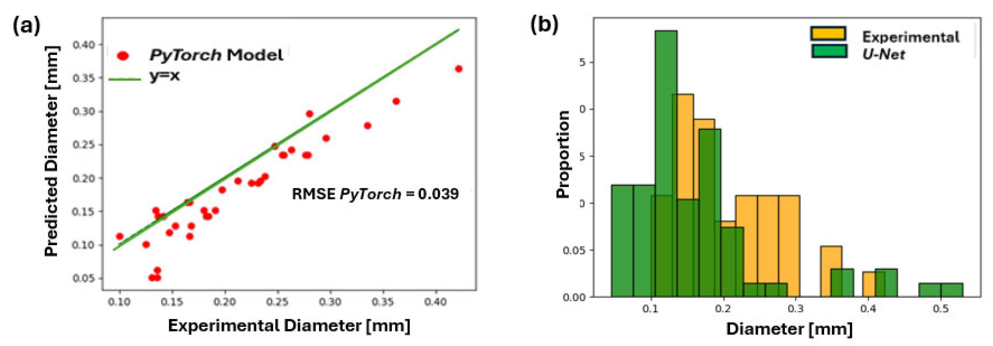
The performance of the U-Net model is summarized in Figure 24 and Figure 25, using the same post-processing applied to the Ilastik model, allowing for direct comparison under consistent evaluation criteria. The Root Mean Square Error (RMSE) values obtained were 0.039 mm for frame 1 (0.160 A) and 0.061 mm for frame 100 (0.190 A). These results indicate a nearly constant discrepancy in bubble diameter predictions, with the deviation being more pronounced for the 0.190 A recording. When evaluated on the same validation set of four images used for the Ilastik model, the U-Net achieved an Intersection over Union (IoU) of 0.68, confirming comparable predictive performance.

9.3.2. Discussion of U-Net Results

In the experiment’s observations, the hydrogen bubble diameters consistently ranged between 0.1 mm and 0.3 mm. Within this range, an RMSE of 0.039 mm at 0.160 A corresponded to a relative error of approximately 20%, while an RMSE of 0.061 mm represented an error of about 30%, assuming a reference diameter of 0.2 mm. These results indicate that the model operates within a persistent margin of error. This discrepancy may arise from labeling inaccuracies during manual data annotation or from image reconstruction errors occurring in the U-Net’s decoding phase. Moreover, the downscaling of the original images from 1024 × 1024 to 512 × 512 pixels likely led to information loss, further compromising measurement precision. It was also observed that the U-Net exhibited a systematic bias, consistently underestimating bubble diameters compared to experimental measurements. This deviation highlights the need for further refinement of both the model architecture and the pre-processing pipeline to achieve more reliable and accurate predictions.

9.4. Comparative Analysis of the Ilastik and U-Net Models

An important consideration in the analysis of bubble segmentation methods is the computational cost. Classical algorithms such as Otsu thresholding and watershed are highly efficient and require minimal processing time, making them suitable for real-time monitoring. In contrast, deep learning-based methods, including U-Net and Mask R-CNN, demand higher computational resources, particularly during training. However, once trained, these models can segment new datasets rapidly. A clear difference in the computational cost was observed between the Ilastik workflow and the U-Net–based segmentation pipeline. Ilastik exhibited considerably lower processing times, with a shorter mean time per frame and minimal hardware requirements. This efficiency arises from its reliance on classical machine learning classifiers and extraction methods, which operate directly on the CPU resources and do not require model training beyond the interactive labeling stage. As a result, Ilastik scales favorably for long image sequences, enabling rapid frame-by-frame segmentation with modest memory usage. On the contrary, the U-Net architecture demands significantly greater computational resources. The training of the model requires GPU acceleration to achieve practical runtimes, and even inference, although faster than training, remains more computationally demanding than Ilastik due to the greater number of convolutional operations and the need to process full-resolution images through a deep encoder–decoder network. The mean time per frame is therefore higher, and the runtime increases appreciably for long sequences.

A computational cost analysis was performed for a 100-frame high-speed imaging sequence to compare the performance of Ilastik and the U-Net segmentation pipeline. U-Net benchmarks were obtained using Google Colab NVIDIA T4 GPU, 16 GB VRAM, 2 vCPUs, 12–25 GB RAM, while Ilastik was executed on a standard CPU workstation Intel Core i7-11700 (Intel Corporation, Santa Clara, California, United States) 32 GB RAM, as Ilastik does not use GPU acceleration. Ilastik’s classical machine learning workflow results in low computational overhead and fast per-frame processing.

Table 1. Metrics values for the computational cost of Ilastik.

Metric	Ilastik (CPU)
Mean Inference Time per Frame	8–15 ms/frame
Total Runtime for 100-frame Sequence	0.8–1.5 s
Peak RAM Usage	1.5–2.0 GB

shows the values for the main evaluation metric for the computational costs of Ilastik.

Ilastik therefore provides near-real-time segmentation even for extended sequences and requires no specialized hardware. Regarding the U-Net computational cost. Although training is performed only once, it represents the largest computational cost in the U-Net workflow.

Table 2. Metrics values for the training computational costs of U-Net.

Metric	U-Net Training (GPU)
Training Time per Epoch (24 images + augmentation)	10–14 s/epoch
Total Training Time (100 epochs)	17–25 min
GPU Memory Usage	3–5 GB VRAM

summarizes the values for the training computational cost of U-Net.

Inference of U-Net was benchmarked separately to isolate the per-frame segmentation cost.

Table 3. Metric values for the U-Net inference for GPU and CPU.

Metric	U-Net Inference (GPU)	U-Net Inference (CPU)
Mean Inference Time per Frame	2.5–4.5 ms/frame	45–70 ms/frame
Total Runtime for 100-frame Sequence	0.25–0.45 s	4.5–7.0 s
Peak RAM Usage	2–3 GB	2–3 GB

summarizes the values for computational cost of U-Net inference for GPU and CPU.

On the T4 GPU, U-Net inference is faster than Ilastik, but this advantage is offset by the substantial training cost and the requirement for GPU availability. In summary, Ilastik offers the fastest overall workflow for a 100-frame sequence with no training cost or GPU being required, being ideal for rapid or repeated analyses. U-Net (GPU) gives fast inference of around 0.3 s per 100 frames, high training cost of approximately 20 min, and requires GPU access for practical performance.

Overall, Ilastik remains the more computationally efficient option for short and long sequences alike, while U-Net offers higher segmentation accuracy at the expense of significantly greater computational resources. The trade-off between accuracy and computational cost should be considered when selecting the appropriate approach for specific experimental scenarios.

The following comparative analysis focuses on qualitative and descriptive aspects of the segmentation approaches applied to the experimental datasets. Metrics such as segmentation quality, handling of overlapping bubbles, and adaptability to varying illumination are discussed to illustrate the characteristics and tendencies of each method without implying benchmarking or claims of superiority.

When comparing the predictions of the Ilastik and U-Net models with the experimental data, (both models demonstrated similar Intersection over Union (IoU) values—0.69 for Ilastik and 0.68 for U-Net—indicating comparable spatial overlap with manually labeled bubbles. The Root Mean Square Error (RMSE) values for individual frames were 0.041 mm (Ilastik) and 0.062 mm (U-Net) for frame 1 at 0.160 A, and 0.024 mm (Ilastik) and 0.039 mm (U-Net) for frame 100 at 0.190 A. For the relative error, frame 1 (≈200 µm bubbles) showed 20% for Ilastik and 31% for U-Net, while frame 100 (≈150 µm bubbles) showed 16% for Ilastik and 26% for U-Net. These values are presented for descriptive purposes and highlight differences in model predictions rather than establishing one method as superior.

Visual inspection of the prediction plots revealed characteristic tendencies of each model:

• Ilastik generally overestimates bubble diameters.
• U-Net generally underestimates bubble diameters.

These tendencies reflect the inherent architectural and training differences between the models. Regarding bubble size distributions, both models exhibited deviations from the experimental data, suggesting systematic biases. For frame 1 (0.160 A), Ilastik captured the overall shape of the distribution reasonably well, though its peak intensity was slightly lower, potentially due to detection of a higher number of small bubbles. For frame 100 (0.190 A), U-Net’s predictions displayed increased variability, emphasizing that RMSE alone does not fully describe qualitative differences in bubble distribution alignment.

Table 4. Comparison of the performance metrics between the Ilastik and U-Net models.

Metric	Frame 1 (0.160 A)	Frame 100 (0.190 A)	Model Comparison
IoU (Intersection over Union)	Ilastik: 0.69	Ilastik: 0.69	≈Equal
	U-Net: 0.68	U-Net: 0.68
RMSE (mm)	Ilastik: 0.041	Ilastik: 0.024	Ilastik better
	U-Net: 0.062	U-Net: 0.039
Relative Error (%)	Ilastik: 20% (200 µm)	Ilastik: 16% (150 µm)	Ilastik better
	U-Net: 31% (200 µm)	U-Net: 26% (150 µm)
Prediction Bias	Ilastik: Overestimation	Ilastik: Overestimation	_
	U-Net: Underestimation	U-Net: Underestimation
Distribution Alignment	Good shape match,	Chaotic, less aligned	Frame 1 Better
	lower Peak

summarizes the observed metrics for both models. The table reports IoU, RMSE, relative error, prediction bias, and distribution alignment descriptively. No quantitative ranking is implied; the values serve to illustrate model tendencies and characteristics.

Overall, both models provide useful insights into bubble dynamics. Ilastik offers a reliable and interpretable segmentation framework with moderate computational requirements, whereas U-Net provides flexibility to capture complex bubble features but requires greater computational resources during training. The choice between models depends on experimental priorities, including processing time constraints and desired qualitative alignment with the observed bubble patterns.

• Main conclusions:

The Ilastik consistently produced lower RMSE values, indicating more precise diameter predictions (Figure 26 and Figure 27). Both models achieved similar IoU scores, meaning that their spatial detection of bubble regions was comparable. Ilastik tended to overestimate, whereas U-Net tend to underestimate bubble sizes. Despite a slightly higher RMSE, Ilastik’s Frame 1 predictions aligned more closely with experimental distributions.

While the Ilastik model outperformed the U-Net based on its lower RMSE and closer alignment with experimental data, this does not imply complete model validation. Even the best-performing Ilastik configuration exhibited a minimum error of 16%, which remains significant. Furthermore, Ilastik’s potential for improvement is limited, primarily dependent on expanding its training dataset-a process constrained by computational resources, given that the current training set comprised only 24 images.

In contrast, the U-Net model presents greater opportunities for enhancement, providing adequate GPU resources. Future improvements could include training directly on high-resolution images (avoiding 512 × 512 downscaling) or implementing patch-based processing, which analyzes smaller image segments individually before recombining them. This strategy preserves high resolution while reducing memory demands, making it particularly suitable for complex image segmentation tasks.

9.5. Predictions of the Hydrogen Bubble Release Frequencies Using the U-Net Model

9.5.1. Presentation of Results

With the bubble release frequency prediction model operational, its performance was evaluated by comparing the number of bubbles predicted by the automated workflow against manually counted values. Manual bubble counts were previously obtained for four distinct experimental conditions: three recordings at current intensities of 0.160 A, 0.190 A, and 0.250 A under non-vibrating conditions, and one recording at 0.190 A with ultrasound-assisted vibration.

To generate predictions, the same U-Net model used for bubble size estimation was applied to all 1504 frames for each experimental video. Following the segmentation stage, tracking was performed using TrackMate, and the resulting dataset was processed with a dedicated exploration algorithm to filter bubbles and compute release frequencies. This procedure enabled a direct comparison between the model-based predictions and the manually obtained experimental counts, providing insight into the reliability of the U-Net-based approach across different electrolysis conditions. Figure 28 illustrates an example of a tracked sequence obtained from the TrackMate tool.

The bubble counts obtained manually and those predicted by the model are summarized in

Table 5. Number of experimentally observed bubbles versus model predictions.

Current	Real Bubble Count	Predicted Bubble Count (U-Net + TrackMate)
0.160 A (Silent)	90	159
0.190 A (Silent)	92	205
0.190 (Piezo)	59	71
0.250 A (Silent)	104	165

.

9.5.2. Analysis of Results

The errors associated with predicting the number of bubbles released from the cathode were found to be substantial, with deviations ranging from 24% to 132%, thereby preventing any meaningful validation of the model for this task. A predominant source of error was the frequent fragmentation of bubble trajectories during tracking. In many frames, a single bubble was incorrectly identified as multiple distinct entities. This occurred because the U-Net segmentations often displayed incomplete white regions, with black intrusions within the predicted bubble areas. These discontinuities caused TrackMate to interpret one bubble as several disconnected components, even when gap-closing options were activated.

This fragmentation behavior was systematic and reflected limitations in the U-Net prediction quality rather than in TrackMate itself. Although TrackMate introduces its own uncertainties—difficult to quantify independently—the decisive factor was the variability and imperfection of the predicted masks across the 1504-frame videos.

Tracking accuracy is highly sensitive to prediction consistency:

• Even one missing bubble in a single frame forces TrackMate to initiate a new track.
• This artificially inflates bubble counts.
• Therefore, this disrupts the computed release frequency.

As previously analyzed in the bubble diameter evaluation, the U-Net model already exhibited uncertainties in segmentation accuracy. These uncertainties became amplified when applied to tracking across long image sequences, where minor inconsistencies accumulate over time. Therefore, when tracking is used to determine the hydrogen bubble release frequency, the segmentation model must provide exceptionally stable predictions across all consecutive frames. Only under such conditions can the method be considered suitable for autonomous analysis of bubble dynamics and for future implementation in reinforcement learning frameworks.

Given the magnitude of the tracking errors, which reached values as high as 132%, the proposed pipeline cannot be considered reliable for a quantitative estimation of the bubble release frequency. These results highlight that the segmentation stability across consecutive frames is critical and that the small segmentation inconsistencies are amplified during tracking. Therefore, the release-frequency results should be interpreted qualitatively rather than quantitatively.

9.6. Discussion

9.6.1. Interpretation of the Segmentation Performance

The comparative analysis between Ilastik and U-Net highlights fundamental differences between classical machine learning workflows and deep learning approaches when applied to experimental electrolysis imaging. Ilastik demonstrated stable segmentation performance with minimal computational cost and limited training data requirements, making it suitable for exploratory studies or scenarios where rapid implementation is needed.

In contrast, the U-Net architecture exhibited higher sensitivity to image variability and training dataset size. Although U-Net has the potential to perform well under large and diverse datasets, its performance in the present study was constrained by the limited number of manually annotated images. As a result, segmentation accuracy was inconsistent across frames, particularly near bubble boundaries.

9.6.2. Impact of Segmentation Errors on the Bubble Tracking

Bubble tracking relies on temporal consistency of segmentation results across consecutive frames. Even small segmentation inaccuracies can propagate and amplify during tracking, leading to significant errors in estimated bubble trajectories and release frequencies. This effect was clearly observed in the present study, where tracking errors reached values exceeding 100%.

These findings demonstrate that segmentation accuracy alone is insufficient to guarantee reliable bubble tracking. Instead, segmentation robustness and temporal coherence must be considered jointly. Consequently, the proposed pipeline cannot yet be considered suitable for quantitative estimation of bubble release frequency, although it remains valuable for qualitative flow visualization.

9.6.3. Physical Interpretation of Bubble Dynamics

Despite the methodological focus of this work, the observed bubble patterns are consistent with known physical mechanisms in alkaline water electrolysis. The relationship between bubble size and release frequency is intrinsically linked to electrochemical operating conditions. An increase in electrical current enhances gas production rates, accelerating bubble growth and increasing the likelihood of coalescence. Ultrasound oscillations promote bubble detachment by reducing adhesion forces and disturbing the boundary layer near the electrode.

Although a detailed parametric study of these effects is beyond the scope of the present work, the image-based observations align with trends reported in the literature, supporting the physical plausibility of the segmentation results. These mechanisms provide a framework for interpreting the observed bubble patterns.

9.6.4. Comparison with the State of the Art

Most previous studies on hydrogen bubble analysis rely on classical threshold-based segmentation techniques and often assume reliable tracking without explicit error quantification. In contrast, the present work provides a direct comparison between classical machine learning (Ilastik) and deep learning (U-Net) approaches using experimental high-speed images, while explicitly quantifying segmentation and tracking errors.

By reporting both successes and limitations, this study contributes a transparent methodological assessment rather than a fully optimized solution.

Table 6. Comparison of this work with representative literature.

Aspect	Literature References	This Work
Image segmentation	Mostly threshold-based [28,29]	Ilastik vs. U-Net
Training dataset	Large or synthetic [9,30,31]	Small experimental dataset
Bubble tracking	Often assumed reliable [9,29,30]	Explicit error analysis
Electrolysis imaging	Static images [32,33,34,35]	High-speed imaging
Limitations discussed	Rarely explicit [30,31,32,33]	Explicit limitations section

summarizes key differences between this work and representative studies reported in the literature, highlighting the methodological advancements and the explicit consideration of segmentation and tracking limitations.

9.7. Limitations of the Study

This study presents several limitations. A major limitation is the reduced size of the manually annotated dataset used to train the U-Net model, consisting of only 24 images. Although data augmentation was applied, the dataset remains insufficient for robust generalization, and the results should not be extrapolated to different electrochemical systems or imaging conditions. Manual labeling was performed by a single annotator, and inter-annotator variability was not assessed, which may introduce subjective biases.

Image downscaling during the pre-processing may have caused potential boundary inaccuracies, particularly for small bubbles. Additionally, inconsistencies in segmentation affected the tracking accuracy, preventing reliable quantitative estimation of bubble release frequency. Background subtraction artifacts associated with electrode porosity may have influenced segmentation near the electrode surface.

These limitations highlight that while the proposed methodology provides qualitative and descriptive insights into bubble dynamics, caution should be exercised when interpreting the results for predictive or fully quantitative purposes.

10. Conclusions

This work presented a comparative evaluation of Ilastik and U-Net for hydrogen bubble segmentation and tracking in high-speed electrolysis images. Ilastik provides a robust and computationally efficient solution for qualitative bubble visualization, whereas U-Net shows potential for capturing complex bubble features but remains strongly dependent on dataset size and annotation quality.

Segmentation inconsistencies and error propagation during tracking prevent either method from being fully validated for quantitative determination of bubble release frequency. Therefore, the findings should be interpreted as exploratory, highlighting both the opportunities and current limitations of machine learning-based approaches for electrolysis imaging.

Future work should focus on expanding the annotated dataset, incorporating multi-annotator labeling, and improving temporal consistency in segmentation to enable more reliable quantitative analysis. Despite the promising potential of automated image segmentation, the current results underscore that further development is needed before these methods can be applied for fully quantitative bubble characterization.

References

1. Part D’énergie Renouvelable Dans la Consommation Finale Brute D’energie en France en 2023. Available online: https://batizoom.ademe.fr/indicateurs/part-des-energies-renouvelables-dans-la-consommation-finale-brute-delectricite (accessed on 11 January 2026).
2. IEA. Share of Renewables in Energy Consumption. Available online: https://www.iea.org/countries/france/renewables (accessed on 11 January 2026).
3. CEA. CLEFS CEA—Number 50/51—HIVER 2004-2005 P25. Available online: https://www.cea.fr/multimedia/Documents/publications/clefs-cea/archives/fr/024a025alleau.pdf (accessed on 11 January 2026).
4. Production De L’Hydrogene. Available online: https://www.connaissancedesenergies.org/fiche-pedagogique/production-de-lhydrogene (accessed on 11 January 2026).
5. CEA. CLEFS CEA—Number 50/51—HIVER 2004-2005 P31. Available online: https://www.cea.fr/multimedia/Documents/publications/clefs-cea/archives/fr/031a033baudouin.pdf (accessed on 11 January 2026).
6. ADEME. La France Pourra-T-Elle Produire Son Propre Hydrogène Vert De Façon Compétitive? Available online: https://hydrogentoday.info/ademe-france-produire-hydrogene-vert/ (accessed on 11 January 2026).
7. Hessenkemper, H.; Starke, S.; Atassi, Y.; Ziegenhein, T.; Lucas, D. Bubble identification from images with machine learning methods. Int. J. Multiph. Flow 2022, 155, 104169. [Google Scholar] [CrossRef]
8. Ronneberger, O.; Fischer, P.; Brox, T. U-Net: Convolutional Networks for Biomedical Image Segmentation. In Medical Image Computing and Computer-Assisted Intervention—MICCAI 2015; Lecture Notes in Computer Science; Navab, N., Hornegger, J., Wells, W., Frangi, A., Eds.; Springer: Berlin/Heidelberg, Germany, 2015; Volume 9351. [Google Scholar] [CrossRef]
9. Colliard-Granero, A.; Gompou, K.A.; Rodenbücher, C.; Malek, K.; Eikerling, M.H.; Eslamibidgoli, M.J. Deep learning-enhanced characterization of bubble dynamics in proton exchange membrane water electrolyzers. Phys. Chem. Chem. Phys. 2024, 26, 14529–14537. [Google Scholar] [CrossRef] [PubMed]
10. Shi, X.; Chen, X.; Cen, L.; Xie, Y.; Yin, Z. Aluminum Electrolysis Fire-Eye Image Segmentation Based on the Improved U-Net Under Carbon Slag Interference. Electronics 2025, 14, 336. [Google Scholar] [CrossRef]
11. Seong, J.H.; Ravichandran, M.; Su, G.; Phillips, B.; Bucci, M. Automated bubble analysis of high-speed subcooled flow boiling images using U-net transfer learning and global optical flow. Int. J. Multiph. Flow 2023, 159, 104336. [Google Scholar] [CrossRef]
12. Patrick, M.J.; Field, C.R.; Grae, L.H.L.; Rickman, J.M.; Field, K.G.; Barmak, K. A comparative analysis of YOLOv8 and U-Net image segmentation approaches for transmission electron micrographs of polycrystalline thin films. APL Mach. Learn. 2025, 3, 036105. [Google Scholar] [CrossRef]
13. Xu, Y.; Zhang, H.; Li, X. Recent Progress in Electrocatalysts for Water Electrolysis. Catalysts 2020, 10, 1422. [Google Scholar] [CrossRef]
14. Goudula-Jopek, A. Hydrogen Production: By Electrolysis; John Wiley and Sons: Hoboken, NJ, USA, 2015. [Google Scholar]
15. Schalenbach, M.; Tjarks, G.; Carmo, M.; Lueke, W.; Mueller, M.; Stolten, D. Acidic or alkaline? towards a new perspective on the efficiency of water electrolysis. J. Electrochem. Soc. 2016, 163, F3197–F3208. [Google Scholar] [CrossRef]
16. Stolten, D.; Emonts, B. Hydrogen Science and Engineering: Materials, Processes, Systems and Technology; Wiley-VCH: Hoboken, NJ, USA, 2016. [Google Scholar]
17. Wilson, S.D.R.; Hulme, A. Effect of bubbles attached to an electrode on electrical resistance and dissolved gas concentration. Proc. R. Soc. Lond. Ser. A Math. Phys. Sci. 1983, 387, 133–146. [Google Scholar] [CrossRef]
18. Matsushima, H.; Nishida, T.; Konishi, Y.; Fukunaka, Y.; Ito, Y.; Kuribayashi, K. Water electrolysis under microgravity: Part 1. Experimental technique. Electrochim. Acta 2003, 48, 4119–4125. [Google Scholar] [CrossRef]
19. Dou, Z.; Rox, H.; Ramos, Z.; Baumann, R.; Ravishankar, R.; Czurratis, P.; Yang, Z.; Lasagni, A.F.; Eckert, K.; Czarske, J.; et al. Scanning Acoustic Microscopy for Quantifying Two-phase Transfer in Operando Alkaline Water Electrolyzer. J. Power Sources 2025, 660, 238575. [Google Scholar] [CrossRef]
20. Rox, H.; Bashkatov, A.; Yang, X.; Loos, S.; Mutschke, G.; Gerbeth, G.; Eckert, K. Bubble size distribution and electrode coverage at porous nickel electrodes in a novel 3-electrode flow-through cell. arXiv 2022, arXiv:2209.11550v2. [Google Scholar] [CrossRef]
21. Silva, J.P.P.R.; Souza, R.R.; Pereira, J.S.; Oliveira, J.D.; Moita, A.S. Synergistic effects of piezoelectric actuators and electrode architecture in alkaline water electrolysis. Sustain. Energy Technol. Assess. 2025, 83, 104667. [Google Scholar] [CrossRef]
22. Ilastik. Ilastik. Available online: https://www.ilastik.org/documentation/pixelclassification/pixelclassification (accessed on 11 January 2026).
23. Hébert, P.; Laurendeau, D. Traitement Des Images (Part 1: Pretreatment). Available online: https://www.scribd.com/document/498672954/Resume-Rtrait-Ement-Image (accessed on 11 January 2026).
24. IBM. Qu’est Ce Qu’une Forêt D’Arbres Décisionnels. 59 Analysis of Bubble Dynamics on Electrodes via High-Speed Image Processing. Available online: https://www.ibm.com/frfr/think/topics/random-forest (accessed on 11 January 2026).
25. PrBenlahmar. Les Réseaux De Neurones Convolutifs. Available online: https://datasciencetoday.net/index.php/en-us/deep-learning/173-les-reseaux-de-neuronesconvolutifs (accessed on 11 January 2026).
26. Taparia, A. U-Net Architecture Explained. Available online: https://www.geeksforgeeks.org/machine-learning/u-net-architecture-explained/ (accessed on 11 January 2026).
27. ImageJ Official Website. TrackMate LAP Trackers. Available online: https://imagej.net/plugins/trackmate/trackers/lap-trackers (accessed on 11 January 2026).
28. Chen, B.; Ekwonu, M.C.; Zhang, S. Deep learning-assisted segmentation of bubble image shadowgraph. J. Vis. 2022, 25, 1125–1136. [Google Scholar] [CrossRef]
29. Babich, A.; Bashkatov, A.; Eftekhari, M.; Yang, X.; Strasser, P.; Mutschke, G.; Eckert, K. Oxygen versus Hydrogen Bubble Dynamics during Water Electrolysis at Microelectrodes. PRX Energy 2025, 4, 013011. [Google Scholar] [CrossRef]
30. Asaoka, K.; Wakuda, K.; Kanemoto, R.; Suwa, H.; Araki, T. Deep learning-based bubble detection with automatic training data generation: Application to the PEM water electrolysis. Trans. JSME 2023, 89, 22-00325. [Google Scholar] [CrossRef]
31. Sinapan, I.; Lin-Kwong-Chon, C.; Damour, C.; Kadjo, J.-J.A.; Benne, M. Oxygen Bubble Dynamics in PEM Water Electrolyzers with a Deep-Learning-Based Approach. Hydrogen 2023, 4, 556–572. [Google Scholar] [CrossRef]
32. Craye, E.J.B. Bubble Quantification in the Near Electrode Region in Alkaline Water Electrolysis. TU Delft Repository. 2023. Available online: https://resolver.tudelft.nl/uuid:f85ef347-0207-4481-999e-a0c87d7a0ca1 (accessed on 11 January 2026).
33. Lee, J.W.; Sohn, D.K.; Ko, H.S. Study on bubble visualization of gas-evolving electrolysis in forced convective electrolyte. Exp. Fluids 2019, 60, 156. [Google Scholar] [CrossRef]
34. Park, J. Study of Bubble Dynamics and Mass Transport in Alkaline Water Electrolysis: Insights from Event-Based Imaging. UC Irvine Electronic Theses and Dissertations. Master’s Thesis, University of California, Irvine, Irvine, CA, USA, 2024. Available online: https://escholarship.org/uc/item/6dh3w0ds (accessed on 11 January 2026).
35. Zerrougui, I.; Li, Z.; Hissel, D. Comprehensive Modeling and Analysis of Bubble Dynamics and its Impact on PEM Water Electrolysis Performance. In Proceedings of the International Conference on Fundamentals and Development of Fuel Cells, Ulm, Germany, 25–27 September 2023. [Google Scholar]
Figure 1. Workflow for bubble image treatment in alkaline electrolysis.
Algorithms 19 00077 g001
Figure 2. Schematic representation of a conventional configuration (a) and a zero-gap configuration (b).
Algorithms 19 00077 g002
Figure 3. General view of the experimental setup and electrochemical cell.
Algorithms 19 00077 g003
Figure 4. Exploded view of the electrochemical cell: (1) Cell housing, (2) Electrical conductor, (3) Neoprene seal, (4) Diaphragm, (5) Electrode, (6) Screw, and (7 and 8) Channels for electrolyte and gas flow [21].
Algorithms 19 00077 g004
Figure 5. Experimental setup for electrolysis observation: (1) Electrochemical cell, (2) Nickel porous electrode, (3) Piezoelectric actuators, (4) High-speed camera, (5) Light projector, (6) Paper sheet.
Algorithms 19 00077 g005
Figure 6. (a) Frame 1 at 0.190 A (silent) and (b) Frame 2 at 0.190 A (silent).
Algorithms 19 00077 g006
Figure 7. Extraction of the background at 0.250 A (silent).
Algorithms 19 00077 g007
Figure 8. (a) Frame 1 at 0.250 A (silent) pre-treated, and (b) Frame 93 at 0.250 A (silent) pre-treated.
Algorithms 19 00077 g008
Figure 9. Diagram of electrolysis image pre-processing.
Algorithms 19 00077 g009
Figure 10. Ilastik interface showing feature selection.
Algorithms 19 00077 g010
Figure 11. Labeled image at 0.250 A (silent condition).
Algorithms 19 00077 g011
Figure 12. (a) Prediction of the Ilastik model for frame 100 at 0.190 A (silent) and (b) Pre-treated frame 100 at 0.190 A (silent).
Algorithms 19 00077 g012
Figure 13. Implementation of data augmentation.
Algorithms 19 00077 g013
Figure 14. Implementation of the class BubbleDataset.
Algorithms 19 00077 g014
Figure 15. Implementation of the encoding and decoding phases.
Algorithms 19 00077 g015
Figure 16. Implementation of the U-Net model training.
Algorithms 19 00077 g016
Figure 17. Evolution of the loss (left) and IoU (right) as a function of the number of epochs.
Algorithms 19 00077 g017
Figure 18. (a) Prediction with PyTorch for frame 1 at 0.130 A (piezo) and (b) Pre-treatment frame 1 at 0.130 A (piezo).
Algorithms 19 00077 g018
Figure 19. Prediction treated with the Analyze Particles module of the Fiji software.
Algorithms 19 00077 g019
Figure 20. User interface of the TrackMate plugin.
Algorithms 19 00077 g020
Figure 21. Measurement errors of bubble diameter obtained through different methods.
Algorithms 19 00077 g021
Figure 22. (a) RMSE for frame 1 at 0.160 A (silent) using Ilastik; (b) bubble diameter distribution for frame 1 at 0.160 A (silent) using Ilastik.
Algorithms 19 00077 g022
Figure 23. (a) RMSE for frame 100 at 0.190 A (silent) using Ilastik; (b) Bubble diameter distribution for frame 100 at 0.190 A (silent) using Ilastik.
Algorithms 19 00077 g023
Figure 24. (a) RMSE for frame 1 at 0.160 A (silent) using U-Net; (b) Distribution of bubbles dimeters for frame 1 at 0.160 A (silent) using U-Net.
Algorithms 19 00077 g024
Figure 25. (a) RMSE for frame 100 at 0.190 A (silent) using U-Net; (b) Distribution of bubble diameters for frame 100 at 0.190 A (silent) using U-Net.
Algorithms 19 00077 g025
Figure 26. (a) RMSE comparison for frame 1 at 0.160 A (silent) between Ilastik and U-Net; (b) Comparison of the bubble diameter distributions for frame 1 at 0.160 A (silent) between Ilastik and U-Net.
Algorithms 19 00077 g026
Figure 27. (a) RMSE comparison for frame 100 at 0.190 A (silent) between Ilastik and U-Net; (b) Comparison of the bubbles diameter distributions for frame 100 at 0.190 A (silent) between Ilastik and U-Net.
Algorithms 19 00077 g027
Figure 28. Tracking hydrogen bubbles using the TrackMate plug-in.
Algorithms 19 00077 g028