Incomplete Judgments in AHP: Transition-Based Approaches, Aggregation Strategies, and Their Impact on Decision Outcomes

Abstract

This paper examines decision-making challenges that arise when information is incomplete, specifically when judgments are missing or unavailable in the context of individual and group applications of the Analytic Hierarchy Process (AHP). Two illustrative examples are provided. The first, adapted from a recently published study in the field of artificial intelligence, demonstrates how different methods for generating missing judgments can affect the outcomes of an individual decision-maker. The second example addresses a real-world problem of allocating farmland among three crops, wheat, corn, and soybeans, using four evaluation criteria: expenses, labor, reliability, and market considerations. In this example, two decision-makers form a group, and their incomplete judgments leave gaps in pairwise comparison matrices at different levels of the hierarchy. The solution incorporates both transition-based approaches (general transition rule and First-Level Transition Rule) and established methods such as Harker’s and van Uden’s. In addition, aggregation of individual judgments (AIJ) is applied where at least one judgment exists, while geometric aggregation is used when multiple judgments are available. This enables prioritization of decision elements in both examples, with particular attention to cases requiring a priori and a posteriori aggregation of individual judgments across hierarchical levels. A critical analysis of the results highlights key differences between methods, revealing ongoing controversies regarding their reliability in practice. Although it is shown that the First-Level Transition Rule method in the presented examples and other authors’ tests outperforms other methods used, the findings suggest that further research is needed to refine and establish more trustworthy procedures for handling incomplete information in AHP applications.

1. Introduction

Decision-making in a group differs from individual decision-making at both the methodological and mathematical levels. When there are multiple decision-makers (DMs), special techniques are typically required to define, analyze, and solve the problem. The basic scenario is whether the decision is made with or without consensus. In the first case, the focus is on organizing the decision-making process, while in the second, it is on synthesizing the individual decisions of group members. Group decision-making is also characterized by numerous sociological, psychological, and other factors, such as the reasons and methods for structuring groups, interest coalitions within and between groups, the predispositions of group members (education, communication culture, personal affinities, and intentions), and so on. Finally, the context of the decision-making process can change, which is characteristic of so-called electoral campaigns and social choice methodologies.

In the Analytic Hierarchy Process (AHP) [1], a well-established decision-making method, a pairwise comparison matrix is a key tool used to evaluate multiple criteria or alternatives by comparing them two at a time. Each cell in the matrix reflects the relative importance or preference of one element over another using a scale (typically 1 to 9). However, it is common to encounter empty or missing cells during the process, especially in early stages of data collection or when decision-makers are unsure about certain comparisons. Filling empty cells is essential for robust and defensible AHP analysis, and therefore scientists continuously work on finding the best methods to preserve coherent and efficient procedures for identifying missing values in comparison matrices.

Key issues in any discussion related to filling empty cells in AHP comparison matrices are understanding the cause of missing values and the implications of empty cells. Empty cells often arise due to incomplete data from experts or stakeholders, complexity or cognitive overload when comparing many decision elements, time constraints in workshops or interviews, and uncertainty or lack of expertise regarding certain comparisons. Leaving cells unfilled can disrupt the consistency and completeness of the matrix, which in turn affects: (a) calculation of priority weights (e.g., using the eigenvector method); (b) calculation of the consistency ratio (CR) measure (which requires a fully populated matrix); (c) reliability and credibility of the decision-making process.

There are many available approaches to fill empty spaces in matrices. The simplest is to ask the decision-maker (DM) again for the missing judgment. This preserves subjectivity and ensures alignment with stakeholder preferences. The other way is to apply the reciprocity rule, e.g., to use the judgment symmetrical to the main diagonal in the matrix and take its reciprocal value.

These are straightforward approaches; however, rarely applicable in reality. More justified is to estimate missing judgment by applying transitivity preferences; a simplified version is that, i.e., if A is preferred over B, and B over C, then A should be preferred over C. The problem is to determine how strong preferences are “strong”, i.e., to discover the weights of A, B, and C.

For example: If A > B (value 3) and B > C (value 4), then A > C can be estimated as 3 × 4 = 12. One can estimate a_ij ≈ a_ik × a_kj ≈ a_iJ. This is sometimes called the derived inference method.

To summarize, while direct input from decision-makers is ideal, several mathematical and logical techniques (transitivity, geometric estimation, and reciprocity) can help complete the matrix when direct input is unavailable. The key is to maintain transparency and consistency throughout the process to preserve the integrity of the final decision-making outcome.

In this paper, we consider a stationary context for group decision-making using AHP:

(a)

The number of group members is K ≥ 2;

(b)

The problem hierarchy is defined with a global goal at the top, a set of criteria at a lower level, and a set of alternatives at the bottom, third level.

(c)

Group members express their preferences regarding individual elements of the hierarchy following AHP rules and using Saaty’s 9-point scale;

(d)

Group members are not required to always express their preferences.

Characteristic (a) distinguishes the group from individual (K = 1) AHP applications. As shown in [2], in group decision-making, the synthesis of evaluations or priorities is performed, which does not occur in individual decision-making. Characteristic (b) is not restrictive, as any more complex hierarchy can be reduced to a basic one with only three levels in the AHP sense [1]. Characteristic (c) declares that in AHP, all comparisons of hierarchical elements are made pairwise. When comparing elements E_i and E_j at a given hierarchical level concerning a given element at a higher level, the DM semantically expresses the intensity of their preference for one element over the other. The verbal assessment is automatically assigned a value a_ij from the linear part of Saaty’s integer scale (1–9), where 1 indicates equal importance of E_i and E_j, and 9 represents an absolute higher importance of E_i compared to E_j. Due to the assumed reciprocity, the intensity of preference of E_j over E_i is a_ji = 1/a_ij, which means that the second part of the scale is nonlinear (1/2–1/9). At the time of evaluation, only those two elements being compared are explicitly important to the DM; all others are considered irrelevant. The use of Saaty’s scale is assumed in further consideration, as the group syntheses presented here are based on it and differ from syntheses using other scales. Characteristic (d) distinguishes cases of group decision-making when all group members provide complete information from cases where some information is missing or unavailable.

If all comparisons are performed properly by the DM, then AHP synthesis is straightforward. However, if the DM for various reasons fails to make some judgments, then there are empty cells in the corresponding local matrices. The first case can be treated as decision-making with complete information, and the other case with incomplete information.

This paper addresses the calculation of missing comparisons in AHP applications. Section 2 provides a review of the relevant literature, followed by Section 3, which offers an extended description of models commonly applied in both individual and group AHP settings, with particular emphasis on group AHP synthesis under conditions of complete and incomplete information. Section 4 presents two illustrative examples of handling incomplete matrices within the AHP framework. The first example considers a single 6 × 6 matrix with one missing judgment, representing an individual decision-making context with a one-level AHP hierarchy. The second example examines a two-level AHP hierarchy with missing judgments at both levels. Here, the group decision-making context is used to demonstrate how different methods for imputing missing data can lead to varying results. Finally, Section 5 summarizes the conclusions, highlighting key insights into the treatment of incomplete information in both individual and group AHP applications.

Appendix A and Appendix B present the algorithms used in deriving the solutions for Examples 1 and 2 in Section 4.

2. Related Research

There are many papers related to the problem of performing computations of priorities of decision alternatives within the framework of the Analytic Hierarchy Process (AHP) [1]. Well-established and scientifically sound, this method is widely used across corporate, governmental, and institutional contexts. It has proven in individual contexts, but most recently also proven as particularly effective in group decision-making. In all cases, participants structure the problem hierarchically and provide pairwise comparisons at each level of the hierarchy. In many papers, the problem of missing judgments in pairwise comparison matrices in AHP is also treated, and there are still controversies which approach is the best and which method offers sufficiently trustful solution in filling the one or more gaps in one or more matrices. Most studies are incomplete because they do not offer broader perspectives on AHP support to the decision-making process itself. That is, most studies treat just one matrix within the AHP hierarchical structure, rarely the whole hierarchy with pairwise comparison matrices at its different levels and outcomes of the synthesis process, which concludes the AHP. The reader is directed to the literature for lists and descriptions of the methods used when there are no missing judgments in the AHP matrices, for instance, in [3,4,5,6,7,8,9,10,11].

In relation to the problem of incomplete information while computing priorities of decision elements, which are previously compared in a pairwise manner respecting the decision element in the upper level of the AHP hierarchy (for instance, criteria vs. goal, or alternatives versus given criterion), it is important to recall that the number of comparisons required in complex scenarios can become overwhelming. As indicated in [12], with nine alternatives and five criteria, the group would need to answer 190 questions, and therefore various methods are examined for simplifying the preference elicitation process. A discussion is presented on three main reasons why one would want to make fewer than the full set of judgments for each of one or more sets of factors in an AHP model: (1) to reduce the time to make judgment; (2) he/she is unwilling to make a direct comparison between two particular elements; and (3) he/she is unsure about some comparisons, The paper introduce a method grounded in the graph-theoretic structure of the pairwise comparison matrix and the gradient of the right Perron vector. Simulations of random matrices are used to demonstrate the effectiveness of this approach.

Two extensions of the AHP methodology are presented in [13], aimed at dealing with incomplete pairwise comparisons and nonlinear ratio scales. Namely, the standard mode of questioning in the AHP requires the decision-maker to complete a sequence of positive reciprocal matrices by answering n(n − 1)/2 questions for each matrix, each entry being an approximation to the ratio of the weights of the n items being compared. This paper presents two extensions of the eigenvector approach of the AHP, which allow the decision-maker to say “I do not know” or “I am not sure” to some of the questions being asked, and to approximate nonlinear functions of the ratios of the weights. In this way, the questioning process can be substantially shortened, and better representations of the responses to certain stimuli may be derived. These two extensions are considered to speed up the elicitation process and provide the analyst with greater flexibility in the modeling of the decision-makers’ responses to the stimuli of comparing decision alternatives. However, several interesting research questions remain. First, what are the appropriate values of a in the power function approach, and if this power law is not applicable, what other functional forms f(w_i/w_j) can be employed in the AHP context? Also, the question of how the techniques discussed in this paper can be extended to deal more efficiently and effectively with the overall hierarchical structure, rather than with a single matrix, remains for future research.

An interesting review of the developments of the AHP presented in [14] includes a discussion on incomplete matrices and methods to fill in missing values. The authors referred to several pair-wise comparisons requested in an AHP three-level hierarchy with eight alternatives and six criteria, and counted that the process requires 183 entries in matrices. This high number can quickly become overwhelming, and comparisons may be entered with a small reflection time in order to speed up the process. Therefore, it has been proposed to enter fewer comparisons, which are well evaluated, than the total number of comparisons, which may be an approximate evaluation. In the discussion part, the authors also state that another reason for an incomplete comparison matrix could be that the decision-maker may not have formed a strong opinion on a particular judgment, and rather than forcing him to give an often-wild guess or to have the entire process slowed down due to one comparison, one can simply skip this question. The authors also refer to the work of Carmone et al. [15] and their Monte Carlo simulation study, where comparisons are deleted from large matrices (rank 10, 15, and 20), and where it has been discovered that one can randomly delete as much as 50% of the comparisons without significantly reducing the quality of results. The authors used the value of consistency index as an efficiency criterion of fulfilling the empty places in the matrices by applying different methods.

Ishizaka et al. [14] also recall that the minimal number of comparisons required is n − 1, one for each row or column of the pairwise comparison matrix, and that the other comparisons are redundant and only necessary to check consistency and possibly improve accuracy. For that purpose, suggested calculations are the application of the transitivity rule of general type, such as a_ij = a_ik·a_km·…·a_vj. In relation to this, worth mentioning are arguments of Harker [13] who claimed that “a natural way to fill in the missing matrix element is to take the geometric average of all the indirectly calculated missing comparisons with the extended transitivity rule”. Furthermore, Harker claims that the drawback of this method is that the number of indirect comparisons grows with the number of alternatives n in such a way that the calculation requires a long processing time. In order to overcome this problem, he proposed to use the eigenvector method for prioritization and to derive weights of decision elements directly without estimating unknown comparisons [13]. Note that this method is described briefly and labeled hereafter in our study as Harker’s method.

To obtain results from AHP, it is necessary to fill in all the elements of the lower or upper triangle of the pairwise matrix. As the number of decision elements in an AHP increases, the number of elements to be mutually (pairwise) compared in certain matrices grows almost quadratically, requiring the decision-maker to perform a large number of comparisons. The paper of Muslim et al. [16] explored the characteristics of consistent 5 × 5 matrices when one of its elements is missing and found that out of 1000 randomly generated matrices, only 31 matrices had a consistency ratio less than the tolerance value 0.10. Although it is not reported which prioritization method is used and how transition rules are controlled within a matrix, the findings suggest that a consistent, complete pairwise matrix tends to exhibit the same characteristics (priority sequence, no rank reversal of decision elements, and consistency index), even with one missing value. However, the authors do not propose a method to fill in empty entries in the matrices while maintaining the consistency parameter.

Faramondia et al. [17] discuss an issue of incomplete pairwise comparison matrices concerning the expression of decision-makers’ preferences in an ordinal and cardinal way. Stating that ordinal information is crucial, there is a bias in the literature in the sense that cardinal models dominate. They suggest a need for an approach based on blending ordinal and cardinal information, and as an illustration of their proposal, two cascading problems are considered: first, ordinal preferences are computed while maximizing an index that combines ordinal and cardinal information, and secondly, a cardinal ranking is obtained by enforcing ordinal constraints. An algorithm is developed to enable the required computations, and several examples are used as a proof of concept. In [18], a special class of preferences, given by a directed acyclic graph, is considered. Incomplete pairwise comparison matrices are considered as partial information available in a graph, that is, for some pairs there are no comparison is given. A weighting method is recommended to satisfy the linear order preservation property, which always results in a ranking such that an alternative directly preferred to another does not have a lower rank. The study concentrates on two well-known prioritization methods, the eigenvector method and the Logarithmic Least Squares Method, to check if they meet this axiom. In conclusion, it is stated that weighting methods break linear order preservation, while the ranking obtained by the eigenvector method depends on the chosen incomplete pairwise comparison representation.

A study of Tekile et al. [19] is presented on the application of the Nelder–Mead algorithm to the constrained “λ_max-optimal completion”. Numerical simulations are performed to analyze its performance while solving the problem of how to optimally complete an incomplete matrix, which commonly appears in AHP applications when an expert, for some reason, may avoid certain judgments while making pairwise comparisons of decision elements. The algorithm numerically minimizes a maximum eigenvalue function, which is difficult to write explicitly in terms of variables, subject to interval constraints. Many numerical simulations are carried out to examine the performance of the algorithm, and the results show that the proposed algorithm can minimize the constrained eigenvalue problem. Provided illustrative examples show the simplex procedures obtained by the proposed algorithm, and how well it fills in the given incomplete matrices.

Navarro et al. [20] address common challenges in sustainability-related decision-making, which often involve numerous and conflicting criteria, stretching the capabilities of traditional multi-criteria decision-making tools. Using the AHP framework, the authors highlight that as the number of criteria increases, so does the complexity of their interrelations, making accurate and reliable judgments more difficult. To address this, the paper introduces a neutrosophic AHP completion method that reduces the number of judgments required from decision-makers. This approach enhances response consistency and accounts for the inherent uncertainty in human reasoning. Applied to a sustainable design problem, the method reduced required comparisons by up to 22% and maintained an average accuracy deviation of under 10% compared to a fully completed conventional AHP matrix.

In Kwiesielewicz and van Uden [21] a brief introduction is given about certain achievements in handling incomplete matrices Authors point to Harker’s method [12] which is based on the eigenvalue method, and the method of Shiraishi et al. [22], which is built on an observation of the coefficients of the characteristic polynomial [6] and can estimate only one missing entry. In [13], Harker proposes to reduce the complexity of the preference eliciting process, and as an illustration, he explains how complex a decision process can be if one has to handle a multi-attribute decision problem with nine alternatives and five criteria, requiring that the expert must answer 190 questions. To simplify the whole process, he proposes to start out with incomplete pairwise comparison matrices and then to complete them most consistently. Kwiesielewicz’s approach [23] assumes that the missing data are in the form of ratios consistent with the result ranking. The approach presented by van Uden [24] is based on the geometric mean method [25] and extracts the missing data from the intermediate comparisons.

Srdjevic et al. [26] addressed the challenge of prioritizing decision elements within the AHP when the available information (judgments) is incomplete. They proposed an approach for filling gaps in pairwise comparison matrices generated during the standard AHP procedure. Specifically, the method reconstructs a missing judgment while ensuring that the reproduced values remain consistent with the same ratio scale used for the elicited judgments. To achieve this, the authors introduced the First-Level Transitivity Rule (FLTR) method. The approach screens entries in the neighborhood of the missing value, then applies scaling (if necessary) and geometric averaging of these entries to estimate the missing judgment. Once completed, the matrix can be used for prioritization through the eigenvector method or other standard techniques. The paper illustrates the method with examples and compares it to existing approaches, particularly Harker’s and Van Uden’s methods, both designed to address incomplete AHP matrices. Results show that all methods achieve a degree of consistency, but the authors argue that FLTR has a unique advantage: it preserves the coherence of the generating process. In other words, every value in the matrix, whether original or reconstructed, derives from the same ratio scale and retains correct semantic meaning. In the present study, the FLTR method is applied alongside Harker’s and Van Uden’s approaches. Additionally, the general transition rule (GTR) method is introduced for comparative purposes, enabling a more comprehensive discussion of the strengths and weaknesses of all four methods.

Several notable methods for addressing the problem of incomplete AHP matrices have been developed by researchers worldwide. These include consistency optimization [27], neural network-based approaches [28], the connecting paths method [29], van Uden’s approximation rule for estimating missing judgments [21,24], and graph representation techniques [30], among others. Simulation results reported in [28] indicated that the connecting paths method performs particularly well for small-sized matrices. In this study, the efficiency of different approaches is also compared, including that of the characteristic polynomial-based method [12] and the revised geometric mean method [13].

The state of current research in the subject area—filling incomplete matrices in AHP—is very rich and includes tens of high-quality papers on the problem under study in this paper. Most recently, Csato [31] presented a review on methods related to the problem of how to choose a completion method for pairwise comparison of matrices with missing entries, based on an axiomatic approach. More interesting studies and theoretical background of the incomplete problem can also be found in papers [32,33,34,35,36].

3. Group AHP Synthesis with Complete and Incomplete Information

3.1. Analytic Hierarchy Process (AHP)

The Analytic Hierarchy Process (AHP), introduced by Thomas L. Saaty in the early 1970s [12], is one of the most widely used multi-criteria decision-making methods in both individual and group settings. It establishes a cardinal preference structure for a set of alternatives with respect to a global goal, using a hierarchy of criteria and sub-criteria, and performs best in hierarchically structured problems. Although not an optimization method, AHP is mathematically well-founded and has been applied extensively in strategic management, finance, resource allocation, trade, equipment selection, and many other fields.

AHP is increasingly used for group decision-making. Its application depends on whether group members act independently or aim for cooperation and consensus. In the first case, preferences are synthesized a posteriori using the standard AHP procedure. In the second, individual assessments are aggregated a priori, and the hierarchy is treated as if evaluated by a single decision-maker. This second approach is also relevant when some group members cannot or choose not to express judgments for all criteria or alternatives, leading to incomplete information that must be processed before group synthesis.

Note that whatever scenario happens, such as dealing with one pairwise comparison matrix, or with more matrices during complete AHP application, deriving priority vectors of analyzed decision elements (criteria, alternatives), has to be performed by using certain prioritization method, for instance EV-eigenvector [1], Cosine Maximization method (CM) [9], Direct Least Squares Method [37], Weighted Least Squares Method (WLS) [37], Logarithmic Least Squares Method (LLS) [38], Logarithmic Least Absolute Value Method (LLAV) [39], Goal Programming Method (GP) [40], Logarithmic Goal Programming Method (LGP) [41], and Fuzzy Preference Programming Method (FPP) [42].

3.2. Synthesis with Complete Information

Assuming that all members (k = 1, 2, …, K) of group G have made all the necessary pairwise evaluations for a given hierarchy, in the AHP methodology, there are two ways to determine the priorities of alternatives to the goal. The first method involves applying AHP individually for each decision-maker (DM) and then aggregating the resulting priority vectors for the alternatives. This procedure is known as the Aggregating Individual Priorities (AIP) method and is characterized by the subsequent synthesis of individual decisions. The second method involves immediately aggregating the individual preference ratings across all levels of the hierarchy, followed by synthesis for a virtual (‘group’) decision-maker in the same way as in individual AHP applications. This type of aggregation is known as the Aggregating Individual Judgments (AIJ) method.

It is worth noting that, in AHP group decision-making, the weights (i.e., “importance”) of individual decision-makers can be incorporated in two principal ways, as discussed in detail by Forman and Peniwati [2] and many subsequent studies. One approach is to assume equal importance for all individuals, while the other introduces a priori differences among them. The latter option is generally difficult to justify and can be applied only after obtaining initial results, for example, when decision-makers can be ranked by demonstrated consistency. A further theoretical alternative, excluding one or more individuals based on external criteria, is also hard to defend in practice.

In our research, we considered both decision-makers to be equally important, assigning them weights of 0.5.

AIP and AIJ methods for group synthesis are described in detail in [2]. Here, we present the relationships necessary for understanding the examples in the next section.

For AIP synthesis, two aggregation methods are commonly used:

Weighted Sum Method (WSM). By his method, the individual priority vectors are additively aggregated. The weights of the alternatives determined by each DM are weighted according to the assigned weight or importance of each DM (which could be equal or different for each DM). The weighted mean of the individual priority vectors is then calculated to obtain the final group priorities.

Mathematically, the WSM value for each alternative is given by:

$$z_i^G={\displaystyle \sum _{k=1}^K{\alpha }_k{z}_i(k)}$$

(1)

where $z_i^G$ is the composite weight (priority) of the alternative A_i, and z_i(k) is the weight (priority) of the alternative A_i assigned by the decision-maker k in the group (k =1, 2, …, K), while α_k is the weight (importance) of decision-maker k. By assumption, individual weights α_k are additively normalized.

This method gives more importance to the priorities of decision-makers who are considered more influential or whose judgments are deemed more reliable.

Weighted Product Method (WPM). This is another approach to aggregating the individual priority vectors. Mathematically, the WPM value for each alternative A_i is calculated as:

$$z_i^G={\displaystyle \prod _{k=1}^K{[z_i(k)]}^{{\alpha }_k}}$$

(2)

The individual weights α_k are also subjected to additive normalization before application of Equation (2). This ensures that the total weight assigned to all members sums to one, preserving proportionality and fairness in the aggregation process. After applying Equation (2), it is necessary to perform additive normalization of the weights assigned to all alternatives. This step ensures that the sum of the weights equals one, maintaining consistency and enabling meaningful comparisons across alternatives.

The geometric mean is particularly useful when the data represent relative comparisons and allows for a more balanced aggregation, especially when dealing with varying scales or magnitudes.

For AIJ synthesis, the aggregation method is as follows: The numerical preference ratings for the elements are aggregated at the local level (for each matrix separately) to create a synthetic set of matrices for a fictitious decision-maker (DM) that represents the group. In other words, after all group members have made the necessary pairwise comparisons of the hierarchy elements, the filled matrices of type A(k) = {a_ij(k)} (k = 1, 2, …, K) are aggregated into corresponding unique matrices for the group G by applying micro-aggregation using geometric averaging at each position (i,j):

$$a_{ij}^G=[{\displaystyle \prod _{k=1}^K{a}_{ij}(k){]}^{1/K}}$$

(3)

The final step of this aggregation is to perform the standard AHP synthesis and obtain the final priority vector, i.e., weights of alternatives.

In syntheses (1)–(3), it is assumed that complete information is available, meaning that all group members have made the necessary evaluations. The difference between AIP (Aggregating Individual Priorities) and AIJ (Aggregating Individual Judgments) is that in the calculation of (1) and (2) for AIP, the so-called local weight vectors (w) for all pairwise comparison matrices in the given hierarchy and the composite weight vector (z) for alternatives (obtained through AHP synthesis, i.e., derived values) are used. On the other hand, in the case of AIJ (Equation (3)), the rating a_ij, which can be considered a priori values concerning the previously mentioned ones, is used.

3.3. Synthesis with Incomplete Information

When some comparison matrices contain empty entries, this refers to decision-making with incomplete information. In this case, different techniques are applied depending on whether all or only partial information is available from the decision-makers. In the case of a single decision-maker (DM), AHP is not applicable a priori because it is not possible to determine the priority vector for at least one matrix. In this case, various techniques could be applied to estimate missing information where empty cells appear in comparison matrices. There is no best solution for this problem, and multiple simulations are required with different sizes of matrices in the decision problem, to eventually come to the conclusion which method could be more “trustworthy” concerning criteria such as consistency, minimum violation, reordering, etc.

There are techniques, more or less reliable, that can be used to complete missing entries. Interested readers may consult for details about some techniques (e.g., [13,14,24,26]). A brief description is given below for the methods used in this study:

• Harker’s method

Harker [12,13] was one of the first who propose how to solve the incomplete matrices problem. In [12], he takes the geometric average of all the indirectly calculated missing comparisons, based on the concept of “connecting path”. Connecting paths implement the general transition rule (GTR) based on the following mathematics: if a_ij (i ≠ j) is missed in a positive reciprocal matrix, a_ij can be determined by a connecting path of size k, CP_k, as follows:

CP_k = a_i,p1a_p1,p2 … a_pk,pj

(4)

The missing element a_ij is the geometric mean of all connecting paths related to a_ij:

$$a_{ij}=\sqrt[q]{{\displaystyle \prod _{k=1}^{q}C{P}_k}}$$

(5)

where CP_k is a connecting path, k defines the number of elements in the connecting path, and q is the number of all possible connecting paths. A major drawback of this method, which can also be named the general transition rule (GTR) method, is that the number of connecting paths can be high for large matrices. For example, for a matrix of size 10, the number of connecting paths is 109,000.

If there is more than one missing entry in the incomplete matrix A(a_ij), Harker in [13] proposed to use an nxn matrix from the partially completed matrix $\tilde{A}({\tilde{a}}_{ij})$, defined as

$${\tilde{a}}_{ij}=\left\{\begin{array}{ccc}1+m_i& if& i=j\\ 0& if& a_{ij} is \mathit{missing}\\ a_{ij}& otherwise& \end{array}\right.$$

(6)

where m_i is the number of missing elements in the i-th row. This method can be named hereafter as Harker’s method.

• Van Uden’s method

Van Uden [24] proposed a method for filling in empty positions in the evaluation matrix of size n. Geometric averaging of the products of existing values in the matrix is applied, while adhering to the principle of transitivity. In the case when only one value a_ik is missing in the matrix, due to symmetry, the reciprocal value a_ki is also missing, and in this case, the missing element a_ik is determined using the Formula (4).

$$a_{ik}=\sqrt[n-2]{{\displaystyle \frac{X}{Y}}}, X={\prod }_{\begin{array}{c}j\\ j\ne k\end{array}}{a}_{ij}, Y={\prod }_{\begin{array}{c}j\\ j\ne i\end{array}}{a}_{kj}$$

(7)

In Formula (7), X represents the product of elements along the i-th row (excluding the k-th column), and Y represents the product of elements along the k-th row (excluding the i-th column).

• FLTR method

The first-order transition rule (FLTR) method proposed by Srdjevic et al. [26] is also aimed at filling in empty positions in the evaluation matrix of size n. It also relies on using Saaty’s 9-point scale (S) and assessing a set of inner products:

$$X=\{{(a_{ij}{a}_{jk})}^{(l)}:i\ne j;j\ne k;i,j,k=1,2,\dots ,n;l=1,2,\dots ,m\}$$

(8)

A set X consists of exactly m = n − 2 different inner products of existing elements in a matrix. There are two possible cases:

• Case 1. If all products in X set by an individual value fall within the range [1/9, 9] in Saaty’s scale, denoted as S, then the approximation of missing element a_ik is computed as a geometric average

  $$a_{ik}^{\prime }={[{\displaystyle \prod _{l=1}^{l=m}{\left(a_{ij}{a}_{jk}\right)}^{(l)}}]}^{1/m}$$

  (9)

This value falls into the range [1/9, 9] and it only remains to round the value to the nearest discrete scale point from the set S. This point is then declared as FLTR generated missing value a_ik from the matrix A.

• Case 2. If at least one of the inner products in X violates the range [1/9, 9] in Saaty’s scale, all inner products have to be additively normalized and then scaled to fall within the scale. For a “distance” R between the upper and lower limit of the scale, normalization and scaling give

  $${(a_{ij}{a}_{jk})}^{(l(s))}=[{(a_{ij}{a}_{jk})}^{(l)}/{\displaystyle {\sum }_{l=1}^{l=m}{(a_{ij}{a}_{jk})}^{(l)}}]\cdot R,l=1,\dots ,m, (m=n-2)$$

  (10)

Geometric averaging of scaled values

$$a_{ik}^{\prime }={[{\displaystyle \prod _{l=1}^{l=m}{\left(a_{ij}{a}_{jk}\right)}^{(l(s))}}]}^{1/m}$$

(11)

produces a value which falls within the range R. Simply matching the nearest discrete value on the scale gives the required missing element a_ik.

Note that in Equations (9)–(11), l is superscript, and l(s) is superscript referring to scaled value.

Remark 1. 

The FLTR method uses one pair within each transitivity chain, resulting in a total of (n − 2) chains, which makes the approach straightforward to implement. Although modern computational technologies allow the use of all possible (or at least the most significant) chains without restrictions on data volume, FLTR remains an efficient and unbiased approach, at least with respect to the selection and inclusion of important chains.

                    ***

In group decision-making settings, there are two basic scenarios:

• Each position in each matrix has at least one evaluation made by any decision-maker: In this situation, the evaluation of one decision-maker is simply adopted as the group’s evaluation, as it is the only available data for that position. When there are multiple evaluations for the same position in the matrix, these evaluations are geometrically averaged (micro-aggregation) to obtain a final group evaluation. Geometric averaging ensures that all group members’ opinions are taken into account, even if the evaluations differ.
• When no decision-maker has expressed a preference for at least one pair of elements E_i and E_j, in this case, AHP is not applicable, because there is insufficient data to calculate priorities for all elements in the hierarchy. This situation is similar to that of a single decision-maker who cannot compare all elements, making it impossible to compute the priority vector for the matrix. The only solution is to apply a technique, as mentioned earlier, to “generate missing values” in some matrices. However, this process can lead to instability and significant inconsistency, making the results unreliable.

In both scenarios of incomplete information, the key approach is to leverage the available data as much as possible and to aggregate it (typically using geometric averaging) when multiple evaluations are present. If certain pairs remain unaddressed (with no evaluations from all group members), recall that AHP synthesis becomes unfeasible for the group, as priorities for those pairs cannot be determined. Unless “generative” techniques are applied in group decision-making with incomplete information, the AIP method is not applicable because there are no composite priority vectors for some members of the group. The problem can be solved by applying AIJ with the available information. Since micro-aggregation at position (i,j) in a given matrix is performed by geometrically averaging the evaluations of those group members who have expressed a preference for element E_i over element E_j at least one decision-maker (DM) must express their preference for the value a_ij (or its reciprocal symmetric element a_ji), and a modified version of Formula (3) is then used.

$$a_{ij}^G=[{\displaystyle \prod _{k\in K}{a}_{ij}(k){]}^{1/M}}$$

(12)

where K denotes the set of group members who have evaluated the pair of elements (E_i, E_j) and M is the number of such members.

The conclusion is that group decision-making with incomplete information requires flexibility, as it is not always possible to have complete comparison matrices. In such cases, micro-aggregation and the use of geometric averages allow for a group decision to be reached, even when some information may be missing.

Worth mentioning is that when entries in one or more matrices within an AHP hierarchy are missing, the results of micro-aggregations should be carefully examined to identify potential biases and to determine whether the conditions for safe use in further computations, such as deriving priority vectors or consistency parameters, are satisfied. An effective approach to reducing possible biases is to consult the participating decision-makers and verify with them whether the micro-aggregated values can be considered reliable or should be adjusted in an acceptable manner (e.g., through consensus).

4. Examples and Discussion

The first example illustrates the application of the general transition rules (GTR) and the First-Level Transition Rules (FLTR) for imputing missing entries in an almost fully consistent pairwise comparison matrix of order six, considered in the context of individual decision-making. For methodological comparison, the outcomes derived from Harker’s and van Uden’s approaches are also reported, and the results obtained by all four methods are subjected to a critical comparative discussion.

The second example illustrates the effect of applying the two transition rules in a group decision-making context and within a complete AHP hierarchy, rather than a single matrix. A real-life problem is addressed of allocating land among three crops, evaluated by two decision-makers acting as a group. Both decision-makers provided incomplete judgments, leaving empty cells in their matrices at different levels of the hierarchy. The solution is obtained not only through the use of transition rules but also by applying aggregation of individual judgments (AIJ) in cells where at least one judgment is available, while in positions with multiple judgments, geometric aggregation is employed.

Example 1. 

Individual decision with incomplete information (single matrix).

The comparison matrix of size 6 × 6 is taken from the data set used in Srđević [43], and presented on the left side in Figure 1. Then, arbitrarily chosen cell a₂₄ (and its symmetrical cell a₄₂) is emptied to obtain an incomplete matrix on the right side of Figure 1.

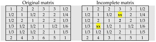
Figure 1. Original and incomplete matrix (Example 1).

Following the FLTR method, relation (8) gives the transitivity pairs X = {(a₂₁·a₁₄), (a₂₃·a₃₄), (a₂₅·a₅₄), (a₂₆·a₆₄)} = {3/2, 1, 4, 3/2}. Because values for all pairs fall into a set (range [1/9, 9]), Case 1 applies. Relation (9) produces the result for missing value a₂₄ = 1.778, which is then rounded to 2 as the nearest discrete value in Saaty’s scale; consequently, a₄₂ is 1/2, Figure 2. The EV method is used to compute priorities and check for consistency parameter CR (which should be less than 0.10). Note that the FLTR method generated a missing entry a₂₄ = 2, with the CR value 0.019; these two values are previously obtained for the original matrix.

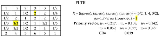
Figure 2. Completed matrix with resulting priorities and CR parameter obtained by FLTR method (Example 1).

By using the GTR method, 13 transition rules are generated randomly to also approximate the missing value a₂₄ (and a₄₂). Better results obtained by this method are shown in Figure 3 for five (out of thirteen) rules labeled as rules 4, 7, 9, 10, 12. The EV method is repeatedly used for each GTR-completed matrix to compute priorities and check for the consistency parameter CR.

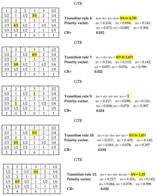
Figure 3. Selected completed matrices with resulting priorities and CR consistency parameter. obtained by GTR method (Example 1).

Note that application of Transition rule 10 led to values (a) a₂₄= 5/3 (≅1.67), close to 2 but without exact semantic value; and (b) consistency ratio CR = 0.018, which is slightly better than the value CR (=0.19) obtained by the FLTR.

Selected general transition rules shown in Figure 3 illustrate how results can differ if transition rules “screen” matrix entries are farther from the empty entry a₂₄. Geometric aggregations of the obtained a₂₄ values should not be close to the result obtained by the FLTR, and the semantic value cannot be exactly obtained as stated in the 9-point scale. Note that it might not be a generally accepted conclusion, but violations of semantic equivalents to numericals again question the validity of the generated outcome.

If Harker’s method (Equation (6)) is applied, corresponding matrices are given in Figure 4. For Harker’s matrix, the derived priority vector and consistency parameter are: w₁ = 0.217; w₂ = 0.106; w₃ = 0.142; w₄ = 0.060; w₅ = 0.078; w₆ = 0.398; CR = 0.018. The result is almost the same as this one obtained by FLTR and GTR (Transition rule 10). Important notice here is that in this case eigenvector method is applied directly to Harker’s matrix, and that there is no estimate of missing judgment a₂₄.

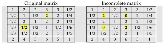
Figure 4. Original matrix (left) and Harker’s matrix (right).

If van Uden’s method is applied (Equation (7)), the matrix on the right side of Figure 5 is obtained, and the result is similar to earlier for FLTR, GTR, and Harker’s methods: w₁ = 0.217; w₂ = 0.105; w₃ = 0.142; w₄ = 0.060; w₅ = 0.078; w₆ = 0.398; CR = 0.018.

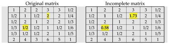
Figure 5. Original matrix (left) and Van Uden’s matrix (right).

Remark 2. 

In either Harker’s or Van Uden’s method, or application of the GTR method, the calculated missing value in the pairwise comparison matrix is not supposed to be explicitly shown; rather, it is directly used for deriving the priority vector. This means that in all these cases, there is no need to have insight into the semantic meaning of the calculated missing value. On the contrary, in the case of the FLTR method, the prioritization is made after the semantic meaning (as defined in Saaty’s scale) is given to the calculated missing value. Recall that in the FLTR method derived value may exactly fit to scale, or it has to be rounded to the nearest value in the scale. In either case, the computed value immediately receives semantic value and only then does the prioritization occur, differently from both Harker’s and Van Uden’s method, or the application of the GTR method. Knowing the exact semantic meaning of the generated missing judgment (as derived by FLTR) could be important to check with the decision-maker because he might have unintentionally skipped that judgment position in the matrix. The other two methods do not offer that opportunity.

Example 2. 

Group decision with incomplete information.

In this example, a complete three-level hierarchy is evaluated in the group context by the AHP, firstly with complete information (all judgments exist), and secondly, with partially missing information (some judgments do not exist).

The real-life problem is defined as follows: Determine the area, concerning the total planting area of an agricultural farm (size 75 hectares), where crops, soybeans, wheat, and corn should be sown. The global goal is to achieve the best allocation of land to crops regarding the criteria: (1) plant production costs; (2) the risk that the crop will fail (reliability); (3) the technical competence of the workforce; and (4) the possibility of market sales (if there is a surplus of products).

The decision has to be made at the group level. Without reducing generality, the assumption is that the group consists of two members (K = 2), labeled as decision-makers DM1 (the first author of this paper) and DM2 (co-author of the paper).

Worth mentioning is that the authors of this paper served as consultants to the farmer in Vojvodina Province in Serbia, helping him to best allocate three crops in season 2023/2024.

The hierarchy has three levels and consists of (top-down view):

Level 1: Goal: Best land allocation

Level 2: Criteria: Costs (C1), Reliability (C2), Workforce (C3), Market (C4)

Level 3: Alternatives: Soybeans (A1), Wheat (A2), Corn (A3)

• Group evaluation of the hierarchy with complete information

The DM1 and DM2 performed all pairwise evaluations (using a 9-point Saaty’s scale), shown in two groups of matrices in Figure 6.

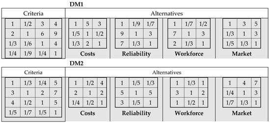
Figure 6. AHP matrices for a three-level hierarchy problem (goal, criteria, alternatives) for decision-makers (DM1 and DM2). Complete information (all judgments present).

Since the information is complete, the group decision can be determined by aggregating the individually obtained priorities of allocating crops. The first two rows in Table 1 are the weights (priority vectors) of the crops obtained by the individual application of AHP for DM1 and DM2; the weights correspond to the percentage of the total area that should be sown by plants. The next two rows in Table 1 present weights (priority vectors) obtained by aggregating individual vectors (weights) of decision-makers (AIP) (Equation (1) for WSM, and Equation (2) for WPM). Finally, the last row contains the group priority vector obtained if geometric micro-aggregation of individual judgments of decision-makers is made (AIJ) (Equation (3)), followed by the standard AHP procedure: (a) prioritization of criteria vs. goal in the first level of hierarchy; and (b) prioritization of alternatives vs. each criterion on the second level of hierarchy. Prioritization at two levels is performed by the eigenvector method.

Table 1. Individual and group weights (priority vectors) for land allocation with complete information.

AHP Methods of Synthesis and Aggregation	Soybeans	Wheat	Corn
	w1	w2	w3
DM1	0.246	0.486	0.268
DM2	0.199	0.610	0.191
Group (AIP/WAM)	0.222	0.548	0.230
Group (AIP/WGM)	0.223	0.549	0.228
Group (AIJ)	0.215	0.564	0.221

The individual evaluations of DM1 and DM2 have only one common ranking: wheat is ranked first. The rankings for soybeans and corn are reversed. Since this is a land allocation problem, cardinal information is more important than the ordering information. Thus, DM1 “believes” that wheat should be sown on about 49% of the available land, while DM2 “believes” that this area should be 61%, and so on.

The group decision, using all three methods of aggregation, results in the same crop ranking as obtained for the DM1: 1. wheat; 2. corn; and 3. soybeans. The percentage values change depending on whether individual priorities are aggregated (AIP) or micro-evaluations (AIJ) are aggregated before prioritization. When AIP is applied, the WAM and WGM results do not differ much, as the group is small (K = 2), and the internal weights for the members are assumed equal (α₁ = α₂ = 0.5). The group decision is that wheat should be sown on about 55% of the land, and so on. When AIJ is applied, the result is, as expected, similar: wheat should be sown on 56% of the land.

• Group evaluation of the hierarchy with incomplete information

Assume that DM1 has not fully expressed his preferences regarding the importance of all elements of the hierarchy. First, in the criteria matrix, DM1 has not provided a rating for the importance of the reliability of yield (C2) relative to the required workforce (C3), and second, he did not specify the relative importance of soybeans (A1) and wheat (A2) concerning the required workforce (C3). In the corresponding matrices, two positions in the upper triangles remain empty: (a) in the criteria matrix, a₂₃ = 6 (as well as symmetrical value a₃₂ = 1/6); and (b) in the workforce matrix, a₁₂ =1/7 (as well as a₂₁ = 7). Matrices for DM1 with complete information are given in Figure 6, and corresponding matrices with incomplete information are presented in Figure 7.

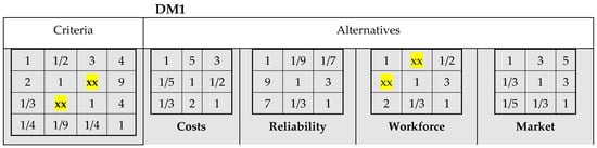
Figure 7. Incomplete matrices for DM1.

For the complete criteria matrix of the DM1 (Cf. Figure 6), the computed priority vector is: w₁= 0.271, w₂ = 0.555, w₃ = 0.123, and w₄ = 0.051; consistency parameter is CR = 0.052.

In case of a missing value a₂₃ (Figure 8, left), application of two general transition rules (GTR 1 and GTR 2) generates value a₂₃ = 9/4 = 2.25 (without semantic meaning) and a₂₃ = 2 (with semantic meaning). Both values are far different from the original value a₂₃ = 6 (Cf. Figure 6). The consistency ratio in both cases is below the tolerance limit of 0.100 (CR = 0.052 and CR = 0.058, respectively), and priority vectors do not differ significantly.

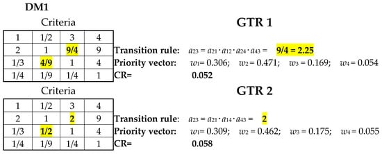
Figure 8. Application of general transition rules to criteria matrix for DM1 (Example 2).

Application of the FLTR method produced the value a₂₃ = 3, Figure 9, with the lowest value of CR = 0.042. Its priority vector differs from those obtained by GTR1 and GTR2. Its Manhattan distance from the original vector is the lowest, that is, 0.120, compared to 0.144 for GTR1 and 0.187 for GTR2.

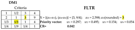
Figure 9. Application of FLTR to criteria matrix for DM1 (Example 2).

Note that priority vectors for the four criteria obtained in cases of GTR and FLTR significantly differ, which may have a strong impact in the later stage of the AHP application. On the other side, for the missing value a₁₂ in a small-sized (3 × 3) matrix for alternatives vs. workforce criterion, both GTR and FLTR calculated the missing value a₁₂ = 1/6, which is the same one as in the original matrix with complete information. The filled (actually reproduced original) small-sized matrix is fully consistent (CR = 0.000), Figure 10.

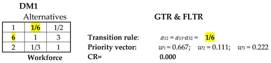
Figure 10. Application of GTR and FLTR to workforce alternatives matrix for DM1 (Example 2).

Remark 3. 

At later stages of AHP synthesis, missing information at the alternatives level may not be as critical, especially when there are only a few alternatives, compared to missing judgments at the higher criteria level, particularly when the number of criteria is large. Our simulations with larger hierarchies (up to 8 criteria and 3 alternatives) confirmed this observation.

Similarly, assume that DM2 has not fully expressed his/her preferences regarding the criteria. For example, if DM2 has not provided a rating for the importance of production costs (C1) relative to the required workforce (C3), then the positions a₁₃ = 1/4 (and a₃₁ = 4) will be emptied in the criteria matrix, Figure 11.

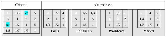
Figure 11. Incomplete criteria matrix for DM2 (Example 2).

Application of GTR and FLTR transition rules generates priority vectors shown in Figure 12. Note that FLTR generated a closer value to the original one (1.00 vs. 0.25; Cf Figure 6), both having the correct semantics value, different from the one generated by application of GTR (1.43).

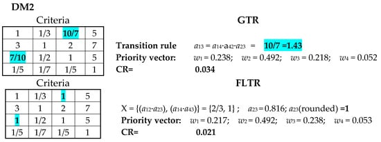
Figure 12. Application of GTR and FLTR rules to criteria matrix for DM2 (Example 2).

Remark 4. 

It is worth noting that for the original criteria matrix of DM2, the computed priority vector is w₁ = 0.152, w₂ = 0.461, w₃ = 0.337, and w₄ = 0.051, with CR = 0.085. This original priority vector differs significantly from the corresponding vectors obtained using GTR and FLTR methods. The higher consistency ratio of the original vector indicates that both GTR and FLTR improved the consistency of the original criteria matrix. Additionally, there is a change in the ordering of w₁ and w_3, and, as in the previous case, the Manhattan distance between the FLTR vector and the original vector is smaller (indicating a closer match) than that between the GTR vector and the original vector.

Since neither DM has defined all of their preferences, the standard AHP synthesis cannot be used in this example to determine their composite vectors, and the AIP method cannot be employed for the group decision. The only option is aggregation using AIJ, as there is at least one defined value for every position in any hierarchy matrix by one of the decision-makers. Recall that in cases where there are two values, their geometric mean is taken.

By applying AIJ, the composite vector of weight values for the crops was obtained: 1. wheat (0.521); 2. soybeans (0.262); and 3. corn (0.218), as shown in Table 2. It can be observed that the share of wheat has decreased compared to the previous cases, but there is also a change in the ranking of the other two crops. Soybeans are ranked higher than corn in this group evaluation, which is an important difference compared to the situation where all preferences are defined.

Table 2. Group priorities for land allocation with incomplete information.

AIJ Aggregation	Soybeans	Wheat	Corn
	w1	w2	w3
Group	0.262	0.521	0.218

Remark 5. 

Regarding this example of group evaluation of the hierarchy with incomplete information, worth to note is that this example illustrates an important and often underestimated phenomenon, which is that incomplete judgments in group AHP can change not only the intensity of preferences but also the ranking of alternatives. In our example, it was shown that the reversal between soybeans and corn when shifting from complete to incomplete information really happened. It would be interesting to explore this outcome more deeply, but with the farmer, a posterior warning him how many implications of the result may be important if there is a missing problem, and force him, for example, to repeat parts of the elicitation process, and provide all judgements in all matrices, especially if they are of small size, like in this practical situation.

5. Conclusions

This study shows that incomplete or missing judgments in the Analytic Hierarchy Process (AHP) significantly affect decision outcomes in both individual and group contexts. This result is well known, and two examples, an AI-inspired case of a single decision-maker and a farmland allocation problem involving multiple decision-makers, additionally demonstrate how different methods yield divergent results. In both examples, transitivity chains are employed to fill in missing elements within the pairwise comparison matrices. Since the transitivity of judgments is not always maintained for objective reasons, the results clearly fluctuated, confirming a long-known fact. To complement the application of transition-based approaches, specifically the General Transition Rule (GTR) and First-Level Transition Rule (FLTR), their results were compared with the results of the methods of Harker and van Uden. In addition, aggregation of individual judgments (AIJ) and geometric aggregation of individual priorities (AIP) were employed to address group decision-making with incomplete data.

The findings highlight that the choice of method, as well as the distinction between a priori and a posteriori aggregation, can alter priority outcomes. The results also confirm that no single approach consistently ensures reliable solutions, underlining the methodological controversies that persist in handling incomplete information in AHP. Probably, this result is the lack of effectiveness criteria, which is discussed in [44].

The presented examples demonstrate that FLTR is more efficient method than GTR in generating missing judgments in comparison matrices. Specifically, FLTR relies on transition rules that primarily (or exclusively) capture the influence of judgments located near the missing value. In contrast, GTR may require a large number of multiplication chains to estimate the missing entry, especially in larger matrices. We also consider it a significant advantage of FLTR that the generated value retains clear semantic meaning, as it is derived directly from the same 9-point scale used for the other judgments in the matrix. GTR, on the other hand, does not necessarily preserve this level of coherence across all judgments, including the imputed one.

It is worth mentioning that in the presented two examples (for a single matrix and multiple matrices within a complete AHP hierarchy), it is shown that the FLTR method outperformed other methods used in this study. However, based on existing methodological controversies and other findings in pertinent literature sources, several avenues for future research are suggested. The development of hybrid models that integrate transition-based rules with established methods could offer a balanced solution between theoretical rigor and computational feasibility. The applicability of these methods should be tested on larger, more complex decision hierarchies to assess their scalability and robustness, while incorporating uncertainty modeling and advanced sensitivity analysis could improve the reliability of results derived from incomplete judgments. Further investigation into aggregation strategies, particularly under varying group dynamics and preference heterogeneity, may provide deeper insights into the robustness of collective decision-making. Advancing research along these lines would help establish more trustworthy and systematic approaches for managing incomplete information in AHP applications.

A specific direction for future research could also be to compare the sensitivity of solutions obtained from a complete AHP hierarchy (rather than a single matrix) within fuzzy and rough set environments, particularly under hesitant group decision-making conditions. Recent researches imply that the sensitivity and robustness of aggregation schemes applied to individual AHP results will be continuously relevant when a larger number of entries are missing across different levels of the hierarchy.

References

- Saaty, T.L. Analytic Hierarchy Process; McGraw-Hill: New York, NY, USA, 1980. [Google Scholar]
- Forman, E.; Peniwati, K. Aggregating individual judgments and priorities with the analytic hierarchy process. Eur. J. Oper. Res. 1998, 108, 165–169. [Google Scholar] [CrossRef]
- Mikhailov, L.; Singh, M.G. Comparison analysis of methods for deriving priorities in the analytic hierarchy process. In Proceedings of the 1999 IEEE International Conference on Systems, Man and Cybernetics, Tokyo, Japan, 12–15 October 1999; pp. 1037–1042. [Google Scholar]
- Mikhailov, L.; Singh, M.G. Fuzzy assessment of priorities with application to the competitive bidding. J. Decis. Syst. 1999, 8, 11–25. [Google Scholar] [CrossRef]
- Lipovetsky, S.; Conklin, W.M. Robust estimation of priorities in the AHP. Eur. J. Oper. Res. 2002, 137, 110–122. [Google Scholar] [CrossRef]
- Srdjevic, B. Combining different prioritization methods in the analytic hierarchy process synthesis. Comp. Oper. Res. 2005, 32, 1897–1919. [Google Scholar] [CrossRef]
- Moreno-Jimenez, J.M.; Aguaron, J.; Escobar, M.T. The core of consistency in AHP-group decision making. Group Dec. Neg. 2008, 17, 249–265. [Google Scholar] [CrossRef]
- Kou, G.; Lin, C. A cosine maximization method for the priority vector derivation in AHP. Eur. J. Oper. Res. 2014, 235, 225–232. [Google Scholar] [CrossRef]
- Tomashevskii, I.L. Optimization methods to estimate alternatives in AHP: The classification with respect to the dependence of irrelevant alternatives. J. Oper. Res. Soc. 2017, 69, 1114–1124. [Google Scholar] [CrossRef]
- Szybowski, J.; Kułakowski, K.; Prusak, A. New inconsistency indicators for incomplete pairwise comparison matrices. Math. Soc. Sci. 2020, 108, 138–145. [Google Scholar] [CrossRef]
- Lin, C.; Kou, G. A heuristic method to rank the alternatives in the AHP synthesis. App. Soft Comp. 2021, 100, 106916. [Google Scholar] [CrossRef]
- Harker, P.T. Alternative modes of questioning in the analytic hierarchy process. Math. Mod. 1987, 9, 353–360. [Google Scholar] [CrossRef]
- Harker, P.T. Incomplete pairwise comparisons in the analytic hierarchy process. Math. Mod. 1987, 9, 837–848. [Google Scholar] [CrossRef]
- Ishizaka, A.; Labib, A. Review of the main developments in the analytic hierarchy process. Expert Syst. Appl. 2011, 38, 14336–14345. [Google Scholar] [CrossRef]
- Carmone, F.J.; Kara, A.; Zanakis, S.H. A Monte Carlo Investigation of Incomplete Pairwise Comparison Matrices in AHP. Eur. J. Oper. Res. 1997, 102, 538–553. [Google Scholar] [CrossRef]
- Muslim, E.; Riansa, I.; Komarudin. Analytic Hierarchy Process (AHP) Pairwise Matrix with One Missing Value. Int. J. Technol. 2017, 7, 1356–1360. [Google Scholar] [CrossRef]
- Faramondi, L.; Oliva, G.; Bozoki, S. Incomplete Analytic Hierarchy Process with Minimum Weighted Ordinal Violations. Int. J. Gen. Syst. 2020, 49, 574–601. [Google Scholar] [CrossRef]
- Csató, L.; Rónyai, L. Incomplete Pairwise Comparison Matrices and Weighting Methods. Fundam. Informaticae 2016, 144, 309–320. [Google Scholar] [CrossRef]
- Tekile, H.A.; Fedrizzi, M.; Brunelli, M. Constrained Eigenvalue Minimization of Incomplete Pairwise Comparison Matrices by Nelder-Mead Algorithm. Algorithms 2021, 14, 222. [Google Scholar] [CrossRef]
- Navarro, I.J.; Martí, J.V.; Yepes, V. Neutrosophic Completion Technique for Incomplete Higher-Order AHP Comparison Matrices. Mathematics 2021, 9, 496. [Google Scholar] [CrossRef]
- Kwiesielewicz, M.; van Uden, E. Ranking Decision Variants by Subjective Paired Comparisons in Cases with Incomplete Data. In Computational Science and Its Applications—ICCSA 2003. Lecture Notes in Computer Science; Kumar, V., Gavrilova, M.L., Tan, C.J.K., L’Ecuyer, P., Eds.; Springer: Berlin/Heidelberg, Germany, 2003; Volume 2669. [Google Scholar] [CrossRef]
- Shiraishi, S.; Obata, T.; Daigo, M. Properties of a positive reciprocal matrix and their application to AHP. J. Oper. Res. Soc. Jpn. 1998, 41, 404–414. [Google Scholar] [CrossRef]
- Kwiesielewicz, M. The logarithmic least squares the generalized pseudoinverse in estimating ratios. Eur. J. Oper. Res. 1996, 93, 611–619. [Google Scholar] [CrossRef]
- van Uden, E. Estimating missing data in pairwise comparison matrices. In Operational and Systems Research in the Face to Challenge the XXI Century, Methods and Techniques in Information Analysis and Decision Making; Bubnicki, Z., Hryniewicz, O., Kulikowski, R., Eds.; Academic Printing House: Warsaw, Poland, 2002; pp. II-73–II-80. [Google Scholar]
- Saaty, T.L. The Analytic Hierarchy Process Series I; RWS Publication: Maidenhead, UK, 1990. [Google Scholar]
- Srdjevic, B.; Srdjevic, Z.; Blagojevic, B. First-level transitivity rule method for filling in incomplete pair-wise comparison matrices in the analytic hierarchy process. App. Math. Inf. Sci. 2014, 8, 459–467. [Google Scholar] [CrossRef]
- Fedrizzi, M.; Giove, S. Incomplete pairwise comparison and consistency optimization. Eur. J. Oper. Res. 2007, 183, 303–313. [Google Scholar] [CrossRef]
- Gomez-Ruiz, A.; Karanik, M.; Peláez, J.I. Estimation of missing judgments in AHP pairwise matrices using a neural network-based model. App. Math. Comp. 2010, 216, 2959–2975. [Google Scholar] [CrossRef]
- Chen, Q.; Triantaphillou, E. Estimating data for multi-criteria decision making problems: Optimization techniques. In Encyclopedia of Optimization; Pardalos, P.M., Floudas, C., Eds.; Kluwer Academic Publishers: Boston, MA, USA, 2001; Volume 2. [Google Scholar] [CrossRef]
- Bozóki, S.; Fülöp, J.; Rónyai, L. On optimal completion of incomplete pairwise comparison matrices. Math. Comp. Mod. 2010, 52, 318–333. [Google Scholar] [CrossRef]
- Csató, L. How to choose a completion method for pairwise comparison matrices with missing entries: An axiomatic result. Approx. Reason. 2024, 164, 109063. [Google Scholar] [CrossRef]
- Dong, Y.; Xu, Y.; Li, H.; Dai, M. A comparative study of the numerical scales and the prioritization methods in AHP. Eur. J. Oper. Res. 2008, 186, 229. [Google Scholar] [CrossRef]
- Ergu, D.; Kou, G.; Peng, Y.; Shi, Y. A simple method to improve the consistency ratio of the pair-wise comparison matrix in ANP. Eur. J. Oper. Res. 2011, 213, 246–259. [Google Scholar] [CrossRef]
- Fan, Z.P.; Jiang, Y.P. A judgment method for satisfying the consistency of the linguistic judgment matrix. Control Decis. 2004, 19, 903–906. [Google Scholar]
- Finan, J.S.; Hurley, W.J. Transitive calibration of the AHP verbal scale. Eur. J. Oper. Res. 1999, 112, 367–372. [Google Scholar] [CrossRef]
- Floriano, C.M.; Pereira, V.; Rodrigues, B.E.S. 3MO-AHP: An inconsistency reduction approach through mono-multi- or many-objective quality measures. Data Technol. Appl. 2022, 56, 645–670. [Google Scholar] [CrossRef]
- Chu, A.; Kalaba, R.; Springam, K. A comparison of two methods for determining the weights of belonging to fuzzy sets. J. Optim. Theory Appl. 1979, 27, 531–541. [Google Scholar] [CrossRef]
- Crawford, G.; Williams, C. A note on the analysis of subjective judgment matrices. Math. Psych. 1985, 29, 387–405. [Google Scholar] [CrossRef]
- Cook, W.D.; Kress, M. Deriving weights from pairwise comparison ratio matrices: An axiomatic approach. Eur. J. Oper. Res. 1988, 37, 355–372. [Google Scholar] [CrossRef]
- Bryson, N. A goal programming method for generating priority vectors. J. Oper. Res. Soc. 1995, 46, 641–648. [Google Scholar] [CrossRef]
- Bryson, N.; Joseph, A. Generating consensus priority point vectors: A logarithmic goal programming approach. Comput. Oper. Res. 1999, 26, 637–643. [Google Scholar] [CrossRef]
- Mikhailov, L. A fuzzy programming method for deriving priorities in the analytic hierarchy process. J. Oper. Res. Soc. 2000, 51, 341–349. [Google Scholar] [CrossRef]
- Srđević, B. Evaluating the Societal Impact of AI: A Comparative Analysis of Human and AI Platforms Using the Analytic Hierarchy Process. AI 2025, 6, 86. [Google Scholar] [CrossRef]
- Saaty, T.; Ergu, D. When is a decision-making method trustworthy? Criteria for evaluating multi-criteria decision-making methods? Inf. Technol. Decis. Mak. 2015, 14, 1171–1187. [Google Scholar] [CrossRef]
Disclaimer/Publisher’s Note: The statements, opinions and data contained in all publications are solely those of the individual author(s) and contributor(s) and not of MDPI and/or the editor(s). MDPI and/or the editor(s) disclaim responsibility for any injury to people or property resulting from any ideas, methods, instructions or products referred to in the content. |
© 2025 by the authors. Licensee MDPI, Basel, Switzerland. This article is an open access article distributed under the terms and conditions of the Creative Commons Attribution (CC BY) license.