Revealing Spatiotemporal Deformation Patterns Through Time-Dependent Clustering of GNSS Data in the Japanese Islands

Abstract

Understanding the spatial and temporal structure of crustal deformation is essential for identifying tectonic blocks, assessing seismic hazard, and detecting precursory deformation associated with major megathrust earthquakes. In this study, we analyze twenty years of continuous GNSS observations from the Japanese Islands to identify coherent deformation domains and anomalous regions using an integrated time-dependent clustering framework. The workflow combines six machine learning algorithms (Hierarchical Agglomerative Clustering, K-means, Gaussian Mixture Models, Spectral Clustering, HDBSCAN and consensus clustering) and constructs a set of deformation-related features including steady-state velocities, strain rates, co-seismic and post-seismic displacements, and spatial distance metrics. Optimal cluster numbers are determined by validity metrics, and the most robust segmentation is obtained using a consensus approach. The resulting spatiotemporal domains reveal clear segmentation associated with major geological structures such as the Fossa Magna graben, the Median Tectonic Line, and deformation belts related to Pacific Plate subduction. The method also highlights deformation patterns potentially associated with the preparation stages of megathrust earthquakes. Our results demonstrate that machine learning-based clustering of long-term GNSS time series provides a powerful data-driven tool for quantifying deformation heterogeneity and improving the understanding of active geodynamic processes in subduction zones.

1. Introduction

The Japanese Islands are some of the most tectonically active regions on Earth, located at the convergence of major lithospheric plates: the Pacific, Philippine, Eurasian (Amurian), and North American (Okhotsk) plates [1]. This complex plate interaction gives rise to high seismicity, active crustal deformation, and the formation of intricate fault-block structures. Understanding the spatial and temporal evolution of these fault-block systems is fundamental for assessing seismic hazard and improving models of crustal dynamics.

Over the past three decades, the deployment of dense GNSS networks, and particularly the GEONET system operated by the Geospatial Information Authority of Japan (GSI), has enabled continuous monitoring of crustal motion with unprecedented temporal and spatial resolution. These long-term GNSS time series reveal steady-state inter-seismic deformation, transient post-seismic relaxation, and co-seismic displacements associated with large subduction earthquakes [2,3] (Figure 1). However, the interpretation of such high-dimensional data remains challenging, as it requires identifying both spatially coherent deformation domains and their evolution through the seismic cycle.

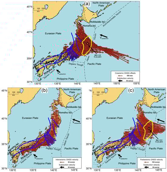
Figure 1. Surface displacements of the Japanese Islands at different stages of the seismic cycle related to the 2011 Tohoku earthquake: (a) co-seismic displacements during the 11 March 2011 Tohoku earthquake; (b) inter-seismic velocities for the period 11.03.2010–10.03.2011; (c) post-seismic velocities for the period 12.03.2011–10.03.2012. Blue lines mark major tectonic faults [4,5]; the semi-transparent blue polygon indicates the Fossa Magna graben [5]. The yellow line outlines the rupture area of the 2011 Tohoku earthquake after [6]. All displacements are shown relative to the Eurasian lithospheric plate.

During the long inter-seismic stage, deformation is largely continuous and reflects elastic strain accumulation driven by plate convergence, resulting in a well-correlated velocity field across the Japanese Islands (Figure 1b). In contrast, the co-seismic stage (Figure 1a) produces highly localized displacements within the vicinity of the rupture area, involving only part of tectonic blocks forming the continental margin. Post-seismic relaxation (Figure 1c) further reveals quasi-independent block motions through afterslip and viscoelastic response [3,7]. These distinct stages of surface motion should therefore imprint characteristic kinematic patterns in GNSS-derived velocity and displacement fields.

Traditional studies of Japan’s tectonic structure have used block models to estimate rotations and inter-block strain, typically relying on predefined geological boundaries [4,8,9,10,11,12,13]. Most of the studies are devoted to identifying tectonic blocks and modeling block motions in particular parts of the Islands, resulting in dozens of small blocks interacting with each other [9,10,11,12,13]. The block models of the whole Islands based on the analysis of GNSS velocity field revealed up to 20 tectonic blocks [4,8]. While these methods have provided valuable insights, they inherently depend on a priori assumptions about the geometry and activity of fault zones.

Modern approaches in studying the tectonic structure of Japanese Islands are based on the clustering methods, providing tectonic segmentation consistent with the block-motion studies [14,15]. Data-driven techniques based on machine learning—particularly clustering analysis—offer a powerful alternative for objectively identifying tectonic domains directly from geodetic observations [14,16,17,18,19,20,21,22,23,24]. Such approaches allow the detection of both stable and transient deformation patterns that may not correspond to previously mapped faults.

Clustering approaches for identifying deformation domains and tectonic blocks are widely used in modern geosciences [16]. The outcome of clustering analyses depends on several factors, including the type of clustering (hard vs. soft), the algorithm (e.g., K-means, hierarchical, DBSCAN), choice of features, validation metrics (Silhouette, Davies–Bouldin, Elbow curve), distance or linkage criteria, and hyperparameter selection. Many studies are devoted to identifying fault block structures in different tectonically active regions, proposing new clustering algorithms and specific linkage criterions, distance metrics, etc., [14,17,18,19,20,21,22]. While most contemporary clustering studies rely on GNSS velocity fields, some valuable perspectives have been gained by applying clustering to strain-rate invariants and rotation-rate fields computed from these velocities [23]. Time-dependent feature space have also been examined as potential sources of additional tectonic information, but primarily in isolated context (for example, co-seismic or steady-state fields analyzed separately) [24].

While inter-seismic deformation patterns have been extensively studied [10,11,12,13], the way in which the spatial structure of deformation changes when co-seismic and post-seismic signals are included remains insufficiently explored. A direct comparison of cluster structures obtained from inter-seismic velocities alone and from an extended dataset incorporating inter-, co- and post-seismic displacements may provide insight into block coupling, segmentation, and stress redistribution following major earthquakes. Such an approach is particularly relevant for Japan, where dense GNSS observations are available before and after the 2003 Tokachi-oki earthquake (Mw 8.3) and the 2011 Tohoku earthquake (Mw 9.0).

Advanced clustering approaches, such as density-based methods (DBSCAN, HDBSCAN) and graph-based or spectral clustering, are particularly suited to identify non-convex domains, diffuse deformation belts, and multi-scale tectonic partitioning [25,26,27,28,29]. Spatiotemporal and trajectory clustering methods can operate on full GNSS time series or temporal embeddings, detecting transient deformation, slow slip, or fault creep [30,31]. Deep learning-based methods (autoencoders, contrastive learning) can extract low-dimensional embeddings directly from raw GNSS time series, capturing subtle transient signals [32].

However, these modern approaches have limitations for tectonic interpretation. Learned embeddings are primarily statistical, making it difficult to relate clusters to geophysical processes, and they may mix tectonic motions with seasonal, hydrological, or anthropogenic signals. In contrast, the regression-derived features used in this study—including inter-seismic velocities, co-seismic offsets, and logarithmic/exponential post-seismic transients—are physically interpretable and directly linked to seismic-cycle mechanics. This allows a clear connection between clustering results and tectonic processes, essential for evaluating block coupling, fault-zone dynamics, and lithospheric segmentation.

The aim of our study is to develop a time-dependent clustering framework for analyzing GNSS-derived deformation parameters in Japan and to evaluate its ability to produce stable clustering results across different initial datasets.

The main contributions and novelty of our study are as follows:

• We propose a time-dependent clustering framework for GNSS time series that incorporates regression-derived, physically interpretable features capturing inter-seismic trends, co-seismic offsets, and post-seismic transients, enabling direct linkage between clustering results and tectonic processes.
• We introduce a robust feature-generation and validation strategy, combined with multiple clustering algorithms, internal validity metrics, and consensus-based stability analysis, ensuring reliable segmentation of deformation patterns in noisy and nonstationary GNSS datasets.
• We apply the proposed methodology to the Japanese Islands, a tectonically complex region, demonstrating how deformation-based cluster boundaries evolve across different stages of the seismic cycle and align with major fault-block structures. The approach is generalizable to other active regions with dense GNSS networks.

2. Seismotectonic Setting

The main seismotectonic patterns of the Japanese Islands region are governed by the nearby subduction zones formed by interaction of major lithospheric plates: Pacific, North American, Eurasian and Philippine Sea [33]. (Figure 2). Recent geotectonic studies also identify smaller regional plates, like Amurian and Okhotsk [1].

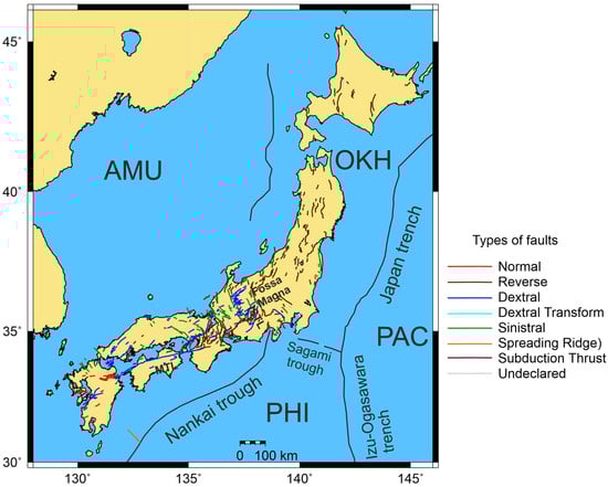
Figure 2. Main active faults of the Japanese Islands [34]. Major plates: PAC (Pacific), PHI (Philippine Sea), OKH (Okhotsk), and AMU (Amurian). Principal inland faults: Median Tectonic Line (MTL) and Itoigawa–Shizuoka Tectonic Line (ISTL).

In this study, we investigate the seismotectonic characteristics of the Japan islands region based on the distribution of regional seismicity according to the ISC catalog [35], focal mechanisms of earthquakes from the Global CMT catalog [36,37], and regional active faults from the GEM Global Active Faults Database [34].

Since the main seismogenic structure of the region is the subducting slab of the Pacific plate, the selection of seismic events was limited to those with source depths shallower than 40 km, in order to focus on the seismotectonic features of the Earth’s crust within the Japanese region (Figure 3).

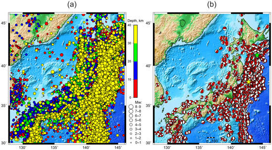
Figure 3. Regional seismicity of the Japanese Islands. (a) Earthquakes with crustal-depth hypocenters from the ISC catalog [35]. (b) Focal mechanisms (shown as beachballs) of earthquakes with $M_w$ > 4.5 according to the gCMT catalog [36,37]. Yellow and green stars indicate the epicenters of the 2011 Tohoku and 2003 Tokachi-oki earthquakes, respectively.

Analysis of the spatial distribution of crustal seismicity and earthquake focal mechanisms reveals several characteristic features. The largest island of the Japanese archipelago, Honshu, is divided by the Fossa Magna graben into two approximately equal parts. The northeastern part of the island is dominated by transcrustal faults of predominantly reverse character, generally oriented subparallel to the oceanic trench (Figure 2). In contrast, the southwestern part is characterized by shallow-focus seismicity (Figure 3), mainly associated with strike-slip faults oriented both subparallel and oblique to the trench axis (Figure 2).

It is also noteworthy that the largest subduction-related earthquake sources are concentrated in the northeastern part of the Japanese archipelago (Figure 3b). During the analyzed period (1996–2016), two major earthquakes with $M_w$ > 8 ruptured the subduction interface in this region—the 2003 Tokachi-oki earthquake ($M_{w}8.3)$ and the 2011 Tohoku earthquake ($M_{w}9.0$). The spatial distribution of regional seismicity (Figure 3b) also reveals several “aseismic” zones surrounded by belts of transcrustal seismicity. These aseismic domains may represent relatively stable crustal blocks.

The deformation field patterns across the Japanese Islands are strongly coupled with the processes of stress accumulation and release in the surrounding subduction zones—commonly referred to as the seismic or earthquake cycle [2,3]. This cycle comprises three main phases: (1) stress accumulation resulting from the interaction between the oceanic and continental lithospheric plates along the subduction interface; (2) stress release during megathrust earthquakes; and (3) post-seismic relaxation. During the stress accumulation phase, tectonic blocks may deform as a consolidated medium, whereas during the co-seismic and post-seismic phases, independent motion of crustal blocks forming the continental margin may occur [38], revealing the actual fault-block structure of the region.

3. Materials and Methods

3.1. GNSS Data

This study utilizes GNSS displacement data from Japan’s GEONET (GNSS Earth Observation Network), one of the densest permanent geodetic networks in the world, operated by the Geospatial Information Authority of Japan (GSI). The dataset comprises time series in the International Terrestrial Reference Frame (ITRF2008) from more than 1400 continuously operating stations covering the period 1996–2016 [39]. A regression analysis of these time series was conducted to derive key parameters describing the kinematic and deformation patterns at each GNSS station, including steady-state motion, seasonal harmonics, co-seismic offsets, and post-seismic relaxation (see Section 3.3.1 for details).

To minimize the influence of large-scale plate motions on the clustering results, we calculated the steady-state plate motions using the NNR-MORVEL56 model [1] (Table S2) and subtracted them from our steady-state velocity components in the ITRF reference frame. The resulting velocity field thus reflects only the steady-state deformation associated with compression along the continental margin and the possible motions of small crustal blocks forming the Japanese Islands. The resulting velocity field is shown in Figure 4b.

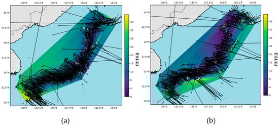
Figure 4. Velocity maps. (a) Initial steady-state GNSS velocities. (b) Modified steady-state GNSS velocities after removing large-scale plate motion using the NNR-MORVEL56 model [1].

3.2. Clustering Algorithm Workflow

The proposed workflow integrates a comprehensive set of unsupervised learning techniques to identify spatiotemporal deformation patterns from GNSS observations in the Japanese Islands. The analysis proceeds through the following main stages (Figure 5):

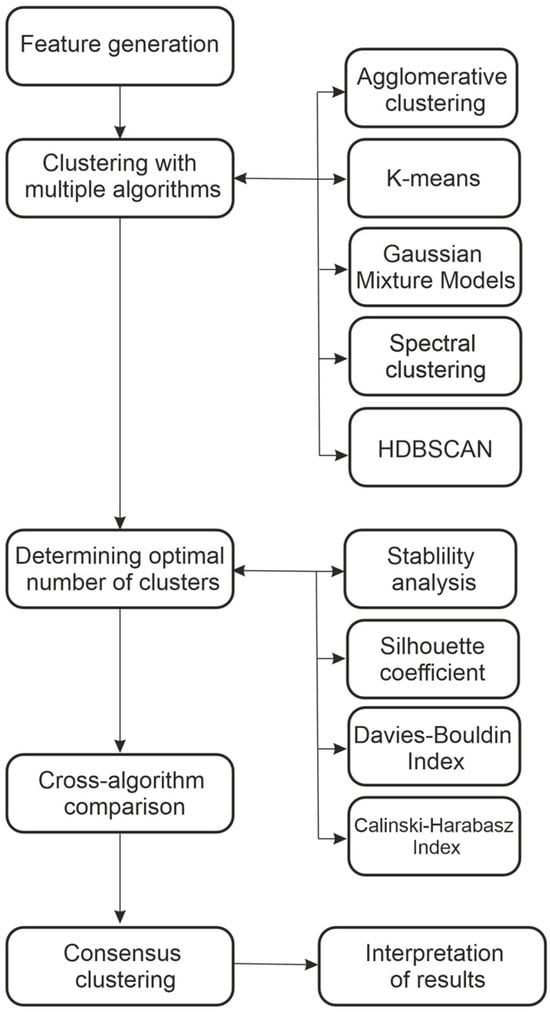
Figure 5. Clustering algorithm pipeline.

• Data preparation and feature engineering.

We constructed the feature vector based on regression-derived parameters that characterize the kinematic and deformation behavior of GNSS stations (see Section 3.3 for details). The resulting features were standardized, examined for pairwise correlations, and subsequently projected into a lower-dimensional space using Uniform Manifold Approximation and Projection for Dimension Reduction (UMAP) [40]. This procedure allows the clustering algorithms to operate on a low-dimensional representation that preserves meaningful local and global structure.

2.

Clustering with multiple algorithms.

Since the key features that best capture deformation patterns associated with regional tectonic blocks are not known a priori, we employ several widely used clustering algorithms (Table 1) to minimize the bias introduced by the choice of a specific method or its hyperparameters. The use of multiple algorithms provides complementary perspectives on the data structure and enables the construction of a consensus clustering that highlights the most stable and tectonically meaningful deformation domains.

Table 1. Description of the clustering algorithms.

Algorithm	Clustering Principle	Metric	Advantages	Limitations
K-means	Minimizes the sum of within-cluster distances	Euclidean	Simple and fast	Performs poorly on non-convex or non-spherical clusters
Gaussian Mixture Models (GMM)	Models clusters as a mixture of probability distributions	Mahalanobis	Flexible cluster shapes; can capture elongated or anisotropic clusters	Sensitive to noise and initialization; may overfit if too many components
Hierarchical Agglomerative Clustering (HAC)	Successively merges clusters using a metric and linkage criterion	Euclidean + Ward’s linkage	Reveals hierarchical structure; natural for tectonic block interpretation	Computationally expensive for large datasets
Spectral Clustering (SPC)	Constructs a similarity graph and clusters the low-dimensional eigenvector embedding	Graph-based similarity	Handles arbitrary cluster shapes; effective on manifold or nonlinear data structures	Requires graph construction; sensitive to choice of similarity parameters
HDBSCAN	Density-based hierarchical clustering with noise identification	Euclidean	Arbitrary cluster Captures clusters of variable density; explicitly identifies noise; robust to outliers	Hyperparameter tuning influences cluster stability; may produce many small clusters

Hierarchical Agglomerative Clustering (HAC) [41] is widely used to segment GNSS velocity fields into tectonic-related domains, effectively capturing hierarchical deformation patterns that naturally reflect the fault-block structure of tectonically active regions, such as the Japanese Islands.

K-Means [42] and Gaussian Mixture Models (GMMs) [43] aim to identify compact clusters within the dataset but differ in their underlying approaches. K-Means is a classical algorithm that minimizes the within-cluster variance of all data points; however, its performance strongly depends on the predefined number of clusters and the initial placement of cluster centers. In contrast, GMM represents a form of soft clustering, where each observation is assigned a probability of belonging to each cluster. This probabilistic formulation is particularly useful for detecting transition zones in deformation fields, such as the boundaries between tectonic blocks.

Spectral Clustering [29] adds a graph-based perspective by first constructing a similarity graph between feature vectors and then using the eigenvectors of the graph Laplacian to embed the data into a space where standard clustering (e.g., K-Means) can effectively detect nonlinear, curved, or manifold-shaped structures. This property is particularly valuable for GNSS-derived features in the Japanese Islands region, where the surface strain field is dominated by continental margin compression associated with subduction, producing elongated, curved, and manifold-like deformation structures.

HDBSCAN [26] provides a complementary density-based viewpoint by building a hierarchy of clusters based on local point density and extracting the most stable cluster configuration. Unlike K-based algorithms, HDBSCAN does not require the number of clusters to be specified in advance, can identify clusters of varying densities, and naturally labels sparse or incoherent observations as noise—an important feature when interpreting deformation fields where measurement gaps, localized transients, or low-signal regions occur.

Together, these complementary algorithms provide multiple perspectives on the clustering of our feature space, offering new insights into the spatiotemporal domains of crustal deformation revealed by the GNSS dataset.

3.

Determination of the optimal number of clusters using combined validity metrics

Since no a priori information is available regarding the number of deformation domains in our dataset, the choice of validation metric—which determines the optimal number of clusters—has a strong influence on the clustering results. Various metrics focus on different aspects of clustering quality. In this study, we employed three metrics that have demonstrated robust performance on synthetic datasets [44]:

• Silhouette Coefficient (SC).
• Davies–Bouldin Index (DBI).
• Calinski–Harabasz Index (CHI).

The Silhouette coefficient [45] is a validity metric focuses on assessing the compactness and separation of clusters. It is formulated as a cumulative sum over all objects:

$$SC={\displaystyle \frac{1}{N}}{\sum }_{i=1}^N\left(b_i-a_i\right)/max(a_i,b_i),$$

(1)

where $a_i$ is the mean distance from i object to all other objects of the same cluster, $b_i$ is the mean distance from i object to all points in the nearest neighboring cluster, N is the total number of objects. The SC tends toward 1 for well-defined clustering solutions, where clusters are both compact and well-separated.

The Davies–Bouldin Index [46] metric quantifies the average ratio of within-cluster scatter to inter-cluster distance for all clusters:

$$\mathit{DBI}={\displaystyle \frac{1}{N}}{\sum }_{i=1}^N\underset{i\ne j}{\max }\left(S_i+S_j/M_{ij}\right),$$

(2)

where k is the total number of clusters, $S_i$ is the average distance between all objects in cluster and its centroid, $M_{ij}$ is the distance between the centroids of clusters i and j. Lower DBI values correspond to compact, well-separated clusters. This property is particularly important for tectonic block identification, since tectonic domains are expected to form spatially coherent regions within the deformation field.

The Calinski–Harabasz Index [47] evaluates the clustering quality by calculating the ratio of between-cluster dispersion to within-cluster dispersion:

$$CHI={\displaystyle \frac{N-k}{k-1}}·{\displaystyle \frac{Tr\left(B_k\right)}{Tr\left(W_k\right)}},$$

(3)

where N is the total number of objects, k is the total number of clusters, $Tr\left(W_k\right)$ is the trace of the within-cluster dispersion matrix, which measures how tight is the distribution of objects $x_i$ of cluster ${Cl}_j$ around its centroid$c_j$:

$$W_k={\sum }_{j=1}^k{\sum }_{x_i\in {Cl}_j}\left(x_i-c_j\right){\left(x_i-c_j\right)}^T,$$

(4)

and $Tr\left(B_k\right)$ is the trace of the between-cluster dispersion matrix, which measures how far are the cluster centroids from the global mean of the dataset:

$$B_k={\sum }_{j=1}^k{n}_j\left(c_j-\overline{x}\right){\left(c_j-\overline{x}\right)}^T,$$

(5)

where $n_j$ is the number of points in jth cluster, $\overline{x}$ is the global mean of all objects.

High CHI values indicate compact and well-separated clusters. In the context of tectonic block identification, a high CHI suggests that clustering successfully distinguishes kinematically distinct and internally coherent deformation domains.

The optimal number of clusters ($K_{opt}$) for each algorithm was determined within a range of K = [2, 30] by identifying the maximum values of SC and CHI, and the minimum of DBI. The results from different criteria were compared to ensure consistency across approaches.

In the next step, we perform a stability analysis of the clustering results for all algorithms. The purpose of this analysis is to assess whether the clustering outcomes remain consistent across multiple runs with varying numbers of clusters (K), slightly modified hyperparameters, or small perturbations added to the input features. To quantify clustering robustness, we apply a statistical test based on the Adjusted Rand Index (ARI) [48], which measures the agreement between two clustering outcomes $U$ and $V$ obtained using different algorithms, parameter settings, or noise realizations:

$$ARI={\displaystyle \frac{RI-\mathbb{E}\left[RI\right]}{max\left(RI\right)-\mathbb{E}\left[RI\right]}},$$

(6)

where RI is the Rand Index [49], representing the proportion of all possible pairs of objects that are assigned consistently (either together or separately) in both clusterings. The term $\mathbb{E}\left[RI\right]$ denotes the expected Rand Index, i.e., the level of agreement that would be observed purely by chance for random cluster assignments with the same number of objects per cluster. The ARI thus corrects for random chance, yielding values close to 1 for highly similar clusterings and near 0 for random or unrelated partitions.

The optimal number of clusters ($K_{opt}$) for each algorithm is compared with the mean ARI values computed over the full range of $K$ each averaged across m repeated runs with varying hyperparameters or small perturbations added to the input features. This comparison ensures that the selected clustering solution corresponds to a stable and reproducible segmentation of the data:

$${ARI}_{UV}\left(K\right)=ARI\left({labels}_U\right(K),{labels}_V(K\left)\right),$$

(7)

The overall stability of the clustering for a given $K$ is than estimated by the mean ARI across all $m$ runs:

$$\overline{ARI}(K)={\displaystyle \frac{2}{m(m-1)}}{\sum }_{U<V}{ARI}_{UV}\left(K\right),$$

(8)

High mean ARI values (0.8–1) indicate stable domains that likely represent coherent tectonic blocks. Moderate ARI values (0.5–0.8) correspond to a mixture of stable domains and uncertain or transitional zones, possibly associated with diffuse deformation. Low ARI values (less than 0.4) suggest that the clustering results are highly sensitive to noise and, therefore, less meaningful in a tectonic sense.

4.

Cross-Algorithm Comparison

To systematically compare all clustering outcomes, we perform a pairwise ARI matrix across all label sets obtained from different algorithms and parameter choices. For each number of clusters K, we compute the pairwise Adjusted Rand Index between the partitions obtained by algorithms a and b:

$${ARI}_{ab}\left(K\right)=ARI\left({labels}_a\right(K),{labels}_b(K\left)\right),$$

(9)

The resulting ARI heatmap visualized the degree of agreement among clustering results. High ARI blocks correspond to consistent partitions detected across methods, indicating reliable underlying structures in the GNSS feature space. Regions of low ARI revealed sensitivity to algorithmic assumptions or parameter choices.

At the last step of cross-algorithm stability analysis, we quantify the average agreement between all algorithms for a given number of clusters K:

$${\overline{ARI}}_{alg}(K)={\displaystyle \frac{2}{n_{alg}\left(n_{alg}-1\right)}}{\sum }_{a<b}{ARI}_{ab}\left(K\right),$$

(10)

where $n_{alg}=3$ is the total number of algorithms involved (K-means, HAC, GMM). The ${\overline{ARI}}_{alg}(K)$ metric provides a measure of the overall consistency among different clustering methods. The final estimate of the optimal number of clusters ($K_{opt}^F$) is determined by maximizing ${\overline{ARI}}_{alg}(K)$ over the explored range of $K$. High values of ${\overline{ARI}}_{alg}(K)$ indicate that different algorithms converge to a similar data partitioning, suggesting that the observed structure reflects intrinsic features of the GNSS velocity field rather than algorithm-specific artifacts. Low ${\overline{ARI}}_{alg}(K)$ values highlight areas of parameters–algorithms space where clustering results are highly sensitive to algorithm-specific assumptions or noise in the feature space.

5.

Consensus clustering

At the final stage of our clustering workflow, we produce the final segmentation of the GNSS data for all clustering algorithms (K-means, HAC, GMM, SPC, HDBSCAN) using final estimate of optimal number of clusters ($K_{opt}^F$).

To combine this obtained clustering results and derive the most stable segmentation of Japanese Islands we also made a consensus clustering [50,51]. The main idea of consensus clustering is to aggregate not the original feature vectors but the label sets $\mathsf{\Pi }=\left\{{\pi }_1,\dots ,{\pi }_C\right\}$already produced by clustering the initial dataset $\mathbb{X}=\left\{x_1,\dots x_N\right\}$ using different algorithms and parameter choices. This is done by aggregating all individual label sets produced by clustering algorithms into a co-association (or similarity) matrix:

$$S_{ij}=S\left(x_i,x_j\right)={\displaystyle \frac{1}{C}}{\sum }_{c=1}^C\mathcal{I}\left({\pi }_c\left(x_i\right)={\pi }_c\left(x_j\right)\right),$$

(11)

where each entry represents the frequency with which two GNSS stations ($x_i\mathrm{and}{x}_j$) were assigned to the same cluster across all algorithms and parameterizations, $C$ is the total number of all clustering outcomes, $\mathcal{I}$ is the indicator function, ${\pi }_c\left(x_i\right)$ and ${\pi }_c\left(x_i\right)$ are the cluster labels assigned to $x_i\mathrm{and}{x}_j$ objects at $c\mathrm{th}$ clustering outcome. The consensus clusters were then derived by applying HAC to the co-association matrix, with the number of clusters set to $K_{opt}^F$ determined previously. The resulting consensus labels represent a robust, ensemble-based synthesis of clustering outcomes, capturing the most stable and tectonically consistent deformation patterns in the Japanese GNSS network.

The resulting clustering maps are then visualized and compared with previously published studies on the fault-block structure of the Japanese Islands and the associated seismotectonic patterns (Figure 2 and Figure 3).

3.3. Feature Vector Construction

The feature generation process is one of the main factors influencing the clustering outcome. In a clustering problem, each object (e.g., a GNSS station) is represented by its numerical counterpart—a feature vector with N components, each reflecting a property of the object that is important for the clustering process. The novelty of our approach is to extend the feature vector describing the clustering objects with additional data emphasizing spatiotemporal behavior of Earth’s lithosphere due to variable strain accumulation.

Since our goal is to capture spatial domains in GNSS data which can be further interpreted as tectonic blocks, we should extract only features reflecting the motion and deformation of these blocks:

• Kinematic features (steady-state velocities, co-seismic offsets, post-seismic decays).
• Deformation features (surface strain parameters).
• Spatial features (distance from trench, elevation).
• Seasonal features (deformation induced by seasonal factors).

All features were derived from the GNSS time series for each station using regression-based recovery algorithms, ensuring consistent parameter estimation across the entire network.

3.3.1. Regression Recovery Problem

To investigate how the seismic cycle affects the mechanical behavior of tectonic blocks and the surface deformation field across the Japanese Islands, we employ a regression-based approach to extract geodynamically meaningful signals from GNSS displacement time series [52]. Our core assumption is that GNSS time series contain separable signals that correspond to physically distinct deformation processes—steady inter-seismic strain accumulation, instantaneous co-seismic offsets, and transient post-seismic relaxation. The primary objective of the regression analysis is to develop an interpretable and statistically robust model capable of decomposing the observed displacements into components representing steady-state, co-seismic, and post-seismic deformation. The regression framework is therefore designed so that each basis function corresponds to a deformation mechanism expected from elastic, viscoelastic, and rate-strengthening models of the seismic cycle. Linear terms capture long-term secular motions related to plate convergence; seasonal harmonics represent hydrological and thermoelastic effects; Heaviside steps model co-seismic displacements; and logarithmic or exponential terms encode post-seismic relaxation (viscoelastic relaxation in upper mantle and frictional afterslip) with physically interpretable decay timescales. Because the model is additive, each estimated coefficient directly measures the strength of its corresponding deformation component at a given GNSS site. This approach integrates statistical modeling with geophysical interpretation, enabling the resulting regression coefficients to serve as informative features for subsequent clustering and machine learning analyses of deformation domains and crustal block dynamics.

The problem is formulated as a supervised learning task where the model seeks a parametric statistical dependence

$$M=\left\{f\left(t,\theta \right)|\theta \in \mathsf{\Theta }\right\},$$

(12)

between the moments of time $t_i\in T$ and the observed values of the time series $y_i\in Y$. Here, θ is a vector of parameters representing contributions of different deformation processes.

Within this formulation, the regression recovery task becomes equivalent to empirical risk minimization:

$$a\left(X^m\right)=\underset{a\in M}{\mathrm{argmin}}Q\left(a,X^m\right),$$

(13)

where

$$Q\left(a,X^m\right)={\displaystyle \frac{1}{m}}{\sum }_{i=1}^m\mathcal{L}\left(a,t_i\right),$$

(14)

is an empirical risk functional, $a=a\left(X^m\right)\in \mathrm{M}$ is a parametric model trained on a dataset $X^m=\left(t_i,y_i\right),i=1,\dots ,m$ and $\mathcal{L}(a,t_i)$ is the loss function, typically formulated as the squared error between predicted and observed displacements.

The displacement model is constructed based on the principle of deformation additivity. Accordingly, the model can be expressed as a linear combination of basis functions:

$$M={\sum }_{j=1}^n{\theta }_j{p}_j\left(T\right),\theta \in {\mathbb{R}}^n,$$

(15)

where $p_j\left(T\right)$ are time-dependent functions forming the feature vector:

$$p\left(t\right)=\begin{array}{c}(1,t,\sin \left(2\pi t\right),\cos \left(2\pi t\right),\sin \left(4\pi t\right),\cos \left(4\pi t\right),H\left(t>T_0\right),\dots ,\\ H\left(t>T_l\right),H\left(t>T_0^{post}\right)·{post}_0\left(t\right),\dots ,\left(t>T_k^{post}\right)·{post}_k\left(t\right))\end{array},$$

(16)

The Heaviside function $H\left(t\right),$models instantaneous displacements (co-seismic offsets) and start times of post-seismic processes, while ${post}_i\left(t\right)$ describes post-seismic relaxation effects, typically parameterized as:

$$post\left(t\right)=\left|\begin{array}{c}\left(\mathit{ln}\left(1+{\displaystyle \frac{t}{{\tau }_a}}\right),-\mathit{exp}\left(-{\displaystyle \frac{t}{{\tau }_b}}\right)\right)\left(I\right)\\ \left(\mathit{ln}\left(1+{\displaystyle \frac{t}{{\tau }_a}}\right),\mathit{ln}\left(1+{\displaystyle \frac{t}{{\tau }_b}}\right),-\mathit{exp}\left(-{\displaystyle \frac{t}{{\tau }_c}}\right)\right)\left(II\right)\\ \left(\mathit{ln}\left(1+{\displaystyle \frac{t}{{\tau }_a}}\right),-\mathit{exp}\left(-{\displaystyle \frac{t}{{\tau }_b}}\right),-\mathit{exp}\left(-{\displaystyle \frac{t}{{\tau }_c}}\right)\right)\left(III\right)\end{array}\right.,$$

(17)

where ${\tau }_a$, ${\tau }_b$, and ${\tau }_c$ are attenuation constants defining the decay rate of nonlinear post-seismic motion.

The complete regression recovery algorithm includes two main phases: data preparation and modeling. The data preparation phase aims to transform raw GNSS time series into clean, quasi-stationary signals suitable for regression analysis. It consists of:

• Trend estimation using a modified robust Theil–Sen method [53], where slopes are estimated between pairs of points separated by one year to account for the annual harmonic. Trend slopes outside two standard deviations from the median are discarded to ensure robustness.
• Outlier detection and cleaning using classical interquartile range (IQR) technique.
• Instantaneous shift detection using existing change-point algorithms with sliding-window optimization [54]. This step identifies co-seismic displacements and defines the time points $T_0,\dots ,T_N$ for modeling.
• Interpolation of missing data using monotonic piecewise cubic interpolation to fill small data gaps [55].

The modeling phase involves sequentially constructing regression models of increasing complexity:

• Stage 1: A piecewise linear model excluding post-seismic terms is used to determine the most suitable optimization method among the Least Squares, Lasso, Bayesian Ridge, and Theil–Sen algorithms. The method with the highest determination coefficient R² is retained as the optimal approach for the subsequent stage of analysis.
• Stage 2: A complete nonlinear model including post-seismic terms is iteratively constructed. The attenuation constants τ are treated as hyperparameters varied between 1 and 300 days. The best-fit model minimizes mean absolute error while maximizing R².

The statistical significance of the final model is evaluated using F-tests on the regression coefficients, ensuring that all estimated components (linear, periodic, co-seismic, post-seismic) are meaningful.

The resulting regression coefficients and post-seismic parameters help us form a high-dimensional feature vector describing the deformation state of each GNSS station. This enriched feature space may include steady-state velocity components, amplitudes of seasonal variations, magnitudes of co-seismic shifts, and relaxation parameters of post-seismic decay. Clustering these feature vectors allows investigation of whether Japan’s crust behaves as a coherent block or partitions into smaller, semi-independent segments during different phases of the seismic cycle.

3.3.2. Feature Engineering

To obtain a compact and tectonically meaningful feature set, we first derive a set of regression-based parameters from each GNSS time series and then construct combined features whose physical interpretation is directly related to crustal kinematics, co-seismic deformation, and transient post-seismic processes (Table 2). This approach ensures that all features are transparent and geophysically interpretable, unlike latent representations produced by deep neural embeddings or autoencoded trajectories. Although the regression model provides annual and semiannual sinusoidal amplitudes and phases, these signals predominantly reflect hydrological and atmospheric loading, not tectonic deformation. To maintain interpretability and avoid introducing noise unrelated to long-term crustal motion, all seasonal features were excluded from further analysis.

Table 2. List of all features used in clustering.

Feature Name	Type of Probability Distribution	Description
DIST	Gaussian-like	Distance from trench (km)
SOURCE_DIST (Tohoku case)	Multimodal	Distance from earthquake source (centroid)
SOURCE_DIST (Tokachi-oki case)	Multimodal	Distance from earthquake source (centroid)
E_DEF	Gaussian-like	N component of steady-state velocity magnitude (m/a)
N_DEF	Gaussian-like, heavy-tailed	E component of steady-state velocity magnitude (m/a)
U_TREND	Gaussian-like, heavy-tailed	Steady-state vertical velocity, (m/a)
N_OFFSET (Tohoku case)	Heavy-tailed, zero-inflated	N component of co-seismic offset
N_OFFSET (Tokachi-oki case)	Long-tailed, zero-inflated	N component of co-seismic offset
E_OFFSET (Tohoku case)	Heavy-tailed, zero-inflated	E component of co-seismic offset
E_OFFSET (Tokachi-oki case)	Long-tailed, zero-inflated	E component of co-seismic offset
U_OFFSET (Tohoku case)	Long-tailed, zero-inflated	U component of co-seismic offset
U_OFFSET (Tokachi-oki case)	Long-tailed, zero-inflated	U component of co-seismic offset
N_LOG_OFFSET (Tohoku case)	Long-tailed, zero-inflated	N component of afterslip offset
N_LOG_OFFSET (Tokachi-oki case)	Long-tailed, zero-inflated	N component of afterslip offset
E_LOG_OFFSET (Tohoku case)	Long-tailed, zero-inflated	E component of afterslip offset
E_LOG_OFFSET (Tokachi-oki case)	Long-tailed, zero-inflated	E component of afterslip offset
N_EXP_OFFSET (Tohoku case)	Long-tailed, zero-inflated	N component of viscoelastic offset
N_EXP_OFFSET (Tokachi-oki case)	Long-tailed, zero-inflated	N component of viscoelastic offset
E_EXP_OFFSET (Tohoku case)	Long-tailed, zero-inflated	E component of viscoelastic offset
E_EXP_OFFSET (Tokachi-oki case)	Long-tailed, zero-inflated	E component of viscoelastic offset
DILATATION (Tohoku case)	Gaussian-like, heavy-tailed	Dilatation strain rate (1/a)
DILATATION (Tokachi-oki case)	Gaussian-like, heavy-tailed	Dilatation strain rate (1/a)
MAX_SHEAR (Tohoku case)	Long-tailed	Max shear strain rate (1/a)
MAX_SHEAR (Tokachi-oki case)	Long-tailed	Max shear strain rate (1/a)
N_OFFSET_IND	binary	Indicator for N_OFFSET
E_OFFSET_IND	binary	Indicator for E_OFFSET
U_OFFSET_IND	binary	Indicator for U_OFFSET
N_LOG_IND	binary	Indicator for N_LOG_OFFSET
E_LOG_IND	binary	Indicator for E_LOG_OFFSET
N_EXP_IND	binary	Indicator for N_EXP_OFFSET
E_EXP_IND	binary	Indicator for E_EXP_OFFSET

Steady-state GNSS velocities were corrected for rigid plate motion using the reference plate model (MORVEL56) [1]. The residual velocities (E_DEF and N_DEF) represent the surface deformation of the continental margin after removing the rigid component. These quantities directly reflect ongoing tectonic strain accumulation and block motions.

Two spatially continuous strain-rate features were computed from the detrended horizontal velocity field following the method of [56]. Velocities were interpolated onto a regular grid under the assumption of locally uniform deformation in the neighborhood of each node. Spatial derivatives of velocity yield the strain-rate tensor components ${\dot{e}}_{xx}$, ${\dot{e}}_{xy}$ and ${\dot{e}}_{yy}$, which were subsequently used to calculate the DILATATION and MAX_SHEAR features:

$$DILATATION={\dot{e}}_{xx}+{\dot{e}}_{yy},$$

(18)

$$MAX\_SHEAR=\sqrt{{4\dot{e}}_{xy}^2+{\left({\dot{e}}_{xx}-{\dot{e}}_{yy}\right)}^2},$$

(19)

These fields highlight zones of compression, extension, and shear partitioning, and therefore serve as key tectonic indicators in the clustering stage.

During the studied period, two major megathrust earthquakes affected the northern Japanese arc: the 2003 Mw 8.3 Tokachi-oku earthquake and the 2011 Mw 9.0 Tohoku earthquake (Figure 2). To evaluate their influence on regional deformation, we construct two independent sets of earthquake-related features, one for each event. For each earthquake we extract co-seismic N, E and U offsets at the earthquake epoch, which reflect immediate elastic deformation due to fault slip. To distinguish “affected” from “unaffected” regions, we introduce binary indicator features for each offset type (Table 2). These encode the spatial footprint of earthquakes and help clustering algorithms avoid treating zero offsets as valid numerical values. from all distinguished offsets using time of earthquake occurrence.

We also constructed four new features related to horizontal components of the afterslip relaxation (log-type motion) [3] occurred in the vicinity of the rupture zone and the viscoelastic relaxation in the upper mantle (exp-type motion) [7]. Since the afterslip process is relatively fast, we construct log-features as cumulative displacements over first 6 months (t = 0.5 year) after earthquake, using regression-derived values of magnitude $a$ and decay ${\tau }_a$ of afterslip process:

$$N\_LOG\_OFFSET=a^N\mathit{ln}\left(1+{\displaystyle \frac{t}{{\tau }_a^N}}\right),$$

(20)

$$E\_LOG\_OFFSET=a^E\mathit{ln}\left(1+{\displaystyle \frac{t}{{\tau }_a^E}}\right),$$

(21)

Viscoelastic relaxation is a very long-lasting process which can last for decades [7]. We construct related features as cumulative displacements for 1-year after the earthquake (t = 1 year):

$$N\_EXP\_OFFSET=b^N\mathit{exp}\left(1+{\displaystyle \frac{t}{{\tau }_b^N}}\right),$$

(22)

$$E\_EXP\_OFFSET=b^E\exp \left(1+{\displaystyle \frac{t}{{\tau }_b^E}}\right),$$

(23)

To further characterize spatial tectonic context, we include two distance-based features DIST and SOURCE_DIST. DIST is a minimum distance from each station to the nearest point on the subduction trench, derived from the NNR-MORVEL56 plate boundaries [1]. This feature helps approximate the gradient of interplate coupling and margin compression. SOURCE_DIST is a great-circle distance from each station to the epicenter of the particular earthquake. This describes spatial attenuation of co-seismic and post-seismic deformation.

Some features, like co-seismic and post-seismic offsets can produce NaN values for GNSS station in the southern part of Japanese Islands, since large earthquakes with M > 8 producing prominent co-seismic and post-seismic occur only in the northern part of the Islands. We introduce special binary features for all co-seismic and post-seismic offset-related features to help clustering algorithms distinguish “affected” from “unaffected” regions and avoid treating zero offsets as valid numerical values.

To prevent overfitting and eliminate scale-related bias, all features were scaled before the clustering process. Before scaling, each feature undergoes a three-step inspection procedure: (1) spatial visualization on a GNSS map to verify tectonic plausibility and identify spurious values (Table S1); (2) histogram analysis to diagnose feature distribution type (Gaussian-like, heavy-tailed, zero-inflated, multimodal) (Table 2); (3) outlier clipping using interquartile range (IQR)-based thresholds or log-IQR rules for long-tailed variables.

To minimize the influence of skewed, zero-inflated, and heavy-tailed feature distributions on the clustering results, we implemented a distribution-specific scaling algorithm. For each feature, we detect whether the data are zero-inflated, long-tailed, or strongly non-Gaussian and applies an appropriate transformation prior to scaling. Zero-inflated variables are separated into zero and non-zero components to prevent distortion during transformation. Features with strong non-Gaussian structure are normalized using a Yeo–Johnson power transform, while positive long-tailed variables are stabilized using a log-transformation. After transformation, all features are standardized using standard Python 3.13.5 functions RobustScaler (median and IQR) or StandardScaler, depending on sensitivity to outliers. Zeros in zero-inflated features are preserved. This strategy yields feature distributions that are more symmetric and comparable in scale, ensuring that clustering distances are not dominated by extreme values or differing units, and ultimately leading to more stable and physically meaningful cluster structures.

To ensure that the clustering analysis is based on deformation parameters that are both statistically robust and tectonically interpretable, we implemented an automated feature quality assessment workflow. After removing purely metadata fields and intermediate time-series diagnostics, we constructed a cleaned feature matrix containing only GNSS-derived deformation features (Table 3 and Table 4). Indicator variables describing the presence of co-seismic and post-seismic offsets were retained for interpretive purposes but excluded from quantitative scoring.

Table 3. Diagnostic metrics for the Tokachi-oki feature set, ordered by Total Score (highest to lowest).

Feature Name	1 *	2 *	3 *	4 *	5 *	6 *	7 *	8 *
DIST	1.338144	0.696363	0.744344	0.035788	0.718728	2.542118	0.948453	0.632770
U_OFFSET	2.084871	0.319584	0.088237	1.000000	0.663177	2.765984	0.958217	0.612423
DILATATION	1.067104	0.821250	0.802787	0.035768	0.557982	1.906709	0.924564	0.609954
U_TREND	1.048173	0.931759	0.762633	0.035777	0.548013	1.585062	0.961651	0.609009
E_OFFSET	4.581508	0.166083	0.302788	1.000000	0.706750	2.962769	0.877303	0.604584
N_LOG	3.799484	0.241624	0.153565	1.000000	0.672246	2.748255	0.954532	0.593988
E_LOG	1.967987	0.355458	0.077848	1.000000	0.590707	2.371712	0.992256	0.593386
E_EXP	2.158059	0.355458	0.080358	1.000000	0.628337	2.704739	0.852540	0.592322
N_OFFSET	8.557780	0.154646	0.391847	1.000000	0.710990	2.182752	0.987196	0.583719
E_DEF	1.860934	0.367814	0.724870	0.035863	0.635883	2.770939	0.958531	0.572536
N_DEF	1.827167	0.367814	0.792594	0.035793	0.659524	2.608442	0.884839	0.567812
N_EXP	4.157669	0.154646	0.155893	1.000000	0.659739	2.905767	0.749217	0.556306
MAX_SHEAR	1.111572	0.871359	0.424776	0.036078	0.675752	1.335335	0.890049	0.546043

* 1—Variance Inflation Factor Score, 2—Redundancy Score, 3—Shape Score. 4—Dispersion Score, 5—Spatial Score, 6—PCA Loading Score, 7—UMAP Stability Score, 8—Total Score.

Table 4. Diagnostic metrics for the Tohoku feature set, ordered by Total Score (highest to lowest).

Feature Name	1 *	2 *	3 *	4 *	5 *	6 *	7 *	8 *
DIST	1.338144	0.696363	0.744344	0.035788	0.718728	2.542118	0.948453	0.632770
U_OFFSET	2.084871	0.319584	0.088237	1.000000	0.663177	2.765984	0.958217	0.612423
DILATATION	1.067104	0.821250	0.802787	0.035768	0.557982	1.906709	0.924564	0.609954
U_TREND	1.048173	0.931759	0.762633	0.035777	0.548013	1.585062	0.961651	0.609009
E_OFFSET	4.581508	0.166083	0.302788	1.000000	0.706750	2.962769	0.877303	0.604584
N_LOG	3.799484	0.241624	0.153565	1.000000	0.672246	2.748255	0.954532	0.593988
E_LOG	1.967987	0.355458	0.077848	1.000000	0.590707	2.371712	0.992256	0.593386
E_EXP	2.158059	0.355458	0.080358	1.000000	0.628337	2.704739	0.852540	0.592322
N_OFFSET	8.557780	0.154646	0.391847	1.000000	0.710990	2.182752	0.987196	0.583719
E_DEF	1.860934	0.367814	0.724870	0.035863	0.635883	2.770939	0.958531	0.572536
N_DEF	1.827167	0.367814	0.792594	0.035793	0.659524	2.608442	0.884839	0.567812
N_EXP	4.157669	0.154646	0.155893	1.000000	0.659739	2.905767	0.749217	0.556306
MAX_SHEAR	1.111572	0.871359	0.424776	0.036078	0.675752	1.335335	0.890049	0.546043

* As in Table 3.

We evaluated the suitability of each feature for further clustering using an automated Total Score (TS) algorithm that integrates several complementary diagnostics. Each feature receives a composite TS computed as mean of multiple normalized statistical, spatial, and manifold-based measures, all implemented using standard methods available in widely used Python 3.13.5 libraries: (1) variance inflation factors (VIFs) for detecting multicollinearity, (2) maximum correlation–based redundancy scores, (3) univariate distribution properties (skewness, excess kurtosis, and zero inflation), (4) dispersion stability derived from robust scale estimates, (5) spatial coherence quantified by Moran’s I, (6) cumulative PCA loading strength reflecting contributions to variance, and (7) UMAP stability, which measures the sensitivity of a low-dimensional manifold representation to the removal of individual features. Table 3 and Table 4 summarize the diagnostic values for each feature, demonstrating that all features surpass the chosen TS threshold of 0.5, corresponding to a moderate level of “goodness,” and can be confidently included in further clustering procedures.

The VIF Score quantifies how strongly a feature can be linearly predicted from all other features. Low values (VIF < 5) indicate weak collinearity and are considered good, whereas values above 10 imply that the feature is highly redundant and should be excluded.

The Redundancy Score measures the degree to which each feature resembles any other feature. It is defined as one minus the highest absolute pairwise correlation. Values close to 1 indicate a truly independent feature, while values near 0 mean that the feature is almost a duplicate of another and therefore not informative.

The Shape Score assesses the statistical distribution of each feature, combining skewness, kurtosis, and zero-inflation diagnostics. High scores (above 0.7) correspond to well-behaved, balanced distributions, whereas low scores (below 0.3) reveal heavy skew, extreme tails, or a large fraction of zeros—all signs of unstable or noisy features.

The Dispersion Score quantifies how much a feature varies relative to its typical magnitude. Features with strong and meaningful variability obtain high scores, while nearly constant or extremely low-variance features receive low scores and are considered uninformative.

The Spatial Score reflects how strongly a feature exhibits spatial structure, measured through spatial autocorrelation. High values indicate consistent geographic patterns that likely reflect real physical processes. Low values indicate spatial randomness, suggesting the feature may be dominated by noise rather than tectonic signal.

The PCA loading Score measures how much a feature contributes to the dominant modes of variability in the dataset. Features with high loadings meaningfully shape the principal components and have strong global importance, while features with very low scores contribute little to the variance and can often be removed without affecting the analysis.

The UMAP Stability Score evaluates the importance of each feature to the underlying nonlinear structure of the data by measuring how much the UMAP embedding changes when the feature is removed. High values mean the feature helps preserve manifold geometry, while low values indicate that dropping the feature does not affect the embedding—marking it as weak or noisy.

To better capture the nonlinear geometry of GNSS-derived deformation features, we apply UMAP [40]—a graph-based manifold learning approach—allowing the clustering algorithms to operate on a low-dimensional representation that preserves meaningful local and global structure more effectively than linear PCA projections. GNSS deformation patterns in subduction regions, like Japanese Islands, often lie on nonlinear manifolds shaped by processes such as co-seismic strain release, inter-seismic strain accumulation, and viscoelastic transients. In this case calculated UMAP embedding is particularly effective at separating stations with different kinematic regimes, even when their raw features overlap in linear space.

4. Results

4.1. Clustering of the Steady-State Velocity Field

We started our clustering analysis by constructing segmentation of the most common type of GNSS feature space, derived from the horizontal components of the steady-state deformation velocity field (N_DEF and E_DEF). These features capture the primary spatial gradients of motion and allow us to distinguish regions with coherent deformation patterns. The resulting clusters delineate areas with similar steady-state motion, which can be interpreted as tectonic blocks or zones of uniform strain accumulation. Clustering of the steady-state velocity field allows one to identify only large-scale deformation domains within the Japanese Islands that reflect the long-term kinematic behavior of the crust. We assume this clustering as a reference for all other segmentations.

The SC (Figure 6a) and DBI (Figure 6b) validity metrics both marks $K$ = 4 as an optimal number of clusters. This is consistent with the assumption about coherent deformation of continental margin during a stable inter-seismic stage of the seismic cycle. Nevertheless, the CHI maximizes only at K = 29, indicating the presence of possible fine structure in GNSS data (Figure 6c). The $\overline{ARI}(K)$ stability index (Figure 6d) reaches high values (0.9–1) for KMeans, HAC and GMM algorithms for $K$ = 2–10 and exceeds 0.7 for all K-based methods for $K$ > 15.

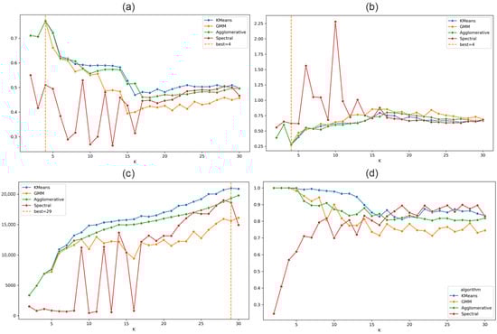
Figure 6. Evaluation metrics for the clustering results for the two-feature vector case. The dashed line marks the optimal number of clusters (K). (a) Silhouette coefficient; (b) Davies–Bouldin index; (c) Calinski–Harabasz index; and (d) stability analysis using the Adjusted Rand Index (ARI).

To assess the cross-algorithm stability and determine the optimal number of clusters, we computed the pairwise ARI heatmap (Figure S1) and the ${\overline{ARI}}_{alg}(K)$ metric (Figure 7). The resulting ARI heatmap indicate consistent partitions at K = 3–5, indicating a stable structure in this area. The ${\overline{ARI}}_{alg}(K)$ values show a clear maximum at K = 4 and K = 9, both reaching approximately 0.81. This suggests that clustering solutions with 4 or 9 clusters are the most consistent across repeated runs and thus represent the most robust structure in the data. For smaller K < 4 or larger K > 9 numbers of clusters, ${\overline{ARI}}_{alg}(K)$ values decrease, indicating less stable or over-fragmented partitions. Thus, ARI-based stability analysis supports selecting K = 4 or K = 9 as the optimal number of clusters for the dataset. The first solution corresponds to large stable clusters due to relatively stable strain accumulation process, whereas the solution with a large number of clusters indicates a possible division of the steady-state deformation into smaller parts.

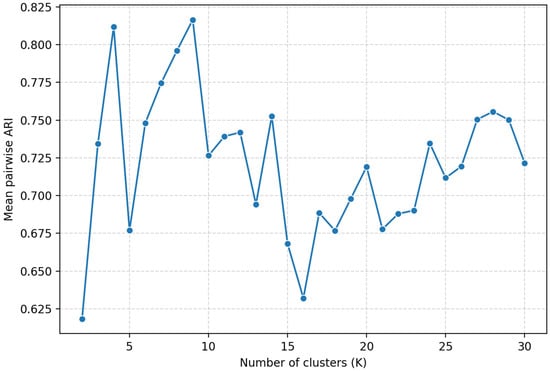
Figure 7. Results of ARI-based estimation of the optimal number of clusters for the two-feature vector case.

We performed clustering using all K-based algorithms (Kmeans, GMM, HAC and SPC), adopting the optimal values of $K_{opt}^F$ = 4 and $K_{opt}^F$ = 9 to derive the possible tectonic segmentation of the Japanese Islands. Clustering solutions in the UMAP-reduced space are shown in Figures S2 and S4 and on the geographic map in Figures S3 and S5. The results from all four clustering K-based techniques are highly consistent in the UMAP-reduced space for $K_{opt}^F$ = 4, in agreement with the high values of ${\overline{ARI}}_{alg}(K)$ metric. For $K_{opt}^F$ = 9 some differences emerge, reflecting alternative ways of subdividing the initial clusters.

To further validate our results, we performed independent clustering using the modern HDBSCAN method. Iterative tuning of HDBSCAN hyperparameters for the two-feature vector case (Table 5) explored a range of minimum cluster sizes and minimum samples to optimize cluster stability and minimize noise points. The tuning indicated that a minimum cluster size of 5–30 and a minimum samples value of 10 provide the most robust clustering, capturing the main data structures while keeping the fraction of unassigned points near 0%. HDBSCAN identified an optimum of K = 4 clusters, supporting the previously determined $K_{opt}^F$ = 4 as the most reliable estimate of clearly distinguished clusters in the Japanese Islands based on the steady-state deformation velocity field.

Table 5. Results of iterative tuning of HDBSCAN parameter for the two-feature vector case.

Minimum Cluster Size	Minimum of Samples	Noise, %	Silhouette Index	Number of Clusters
5	10	0	0.770355	4
10	10	0	0.770355	4
15	10	0	0.770355	4
20	10	0	0.770355	4
30	10	0	0.770355	4
10	1	3.47	0.718274	19
5	5	0	0.710441	5
10	5	0	0.710441	5
15	1	0	0.710441	5
15	5	0	0.710441	5
20	1	0	0.710441	5
20	5	0	0.710441	5
30	1	0	0.710441	5
30	5	0	0.710441	5
5	1	7.06	0.535501	84

We then collected all labels from the K-based and HDBSCAN clustering outcomes to construct a co-association matrix and perform consensus clustering for $K_{opt}^F$ = 4. Comparison of the consensus clustering results with the HDBSCAN outcomes shows a high degree of similarity in both the UMAP-reduced space (Figure 8) and the geographic map (Figure 9), highlighting the advantage of HDBSCAN in handling noisy GNSS data for steady-state deformation rates. Both methods clearly identify trench-parallel clusters associated with the gradual decrease in strain accumulation toward the continent, accurately define boundaries along the Median Tectonic Line (MTL) and the Itoigawa-Shizuoka Tectonic Line (ISTL) (Figure 1 and Figure 2), and distinguish a cluster near the future source region of the 2011 Tohoku earthquake (Figure 3 and Figure 9) revealing the anomaly in the strain accumulation process. The obtained segmentation of the Japanese Islands supports the assumption of two types of deformation patterns along the trench. Northeastern part of Honshu and Hokkaido Islands deform near uniformly during the stable inter-seismic stage of seismic cycle, thus accumulating high amounts of elastic stresses that is later released during megathrust earthquakes. In contrast, the southwestern part of Japanese Islands is characterized by a more intricate tectonic structure, where smaller tectonic blocks deform quasi-independently and contribute to a more heterogeneous strain field.

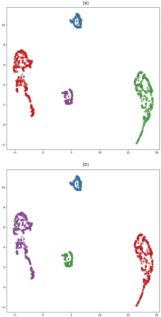
Figure 8. Clustering solutions in the UMAP-reduced space for the two-feature vector case (number of clusters set to 4). Panels show results from (a) Consensus clustering, (b) HDBSCAN.

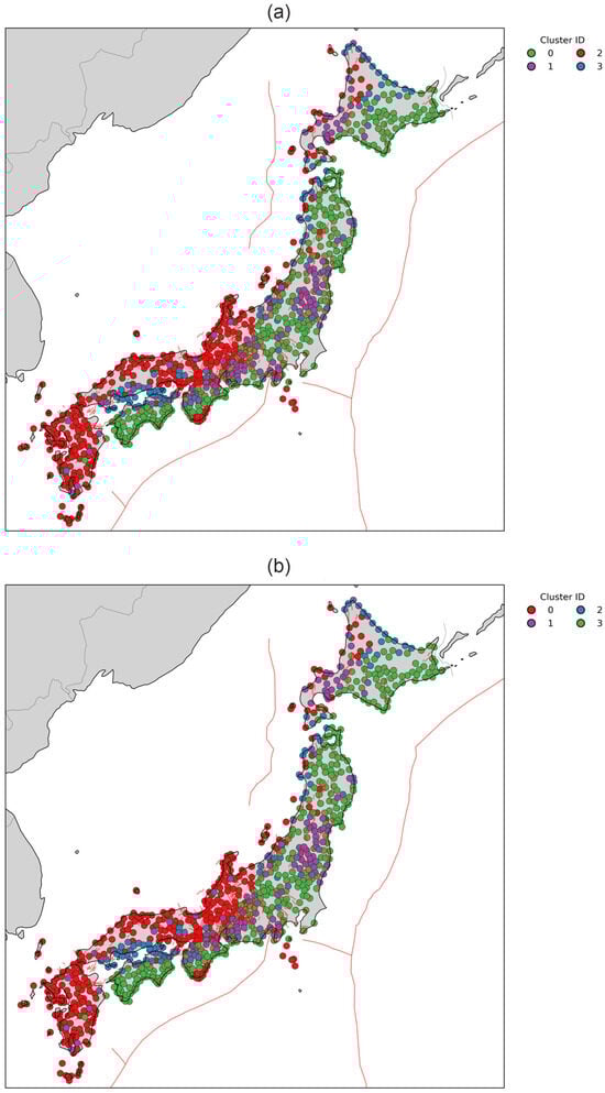
Figure 9. Geographic distribution of clustering results obtained for the two-feature vector case. (number of clusters is set to 4). Panels show results from (a) Consensus clustering, (b) HDBSCAN.

4.2. Clustering of the Complete Feature Vector for the Tokachi-Oki Case

In the next stage of our clustering analysis, we examined the segmentation obtained from the full feature vector, which includes both strain-rate and offset-related features associated with the 2003 Tokachi-oki earthquake (Figure 3). This Mw 8.3 event occurred offshore along the Pacific coast of Hokkaido. Owing to the relatively compact source geometry, the earthquake-related strain accumulation and co-seismic–post-seismic deformation signals are largely confined to Hokkaido Island and its nearest vicinity.

The SC (Figure 10a) and DBI (Figure 10b) validity metrics both marks $K$ = 2 as an optimal number of clusters. This is consistent with the assumption about coherent deformation of continental margin during a stable inter-seismic stage of the seismic cycle. Nevertheless, the CHI maximizes only at K = 30, indicating the presence of possible fine structure in GNSS data (Figure 10c). The $\overline{ARI}(K)$ stability index (Figure 10d) shows less consistency than in the two-feature case, reaching relatively high values (>0.8) within the range K = 12–20, further supporting the notion of potential multi-scale segmentation in the full feature space.

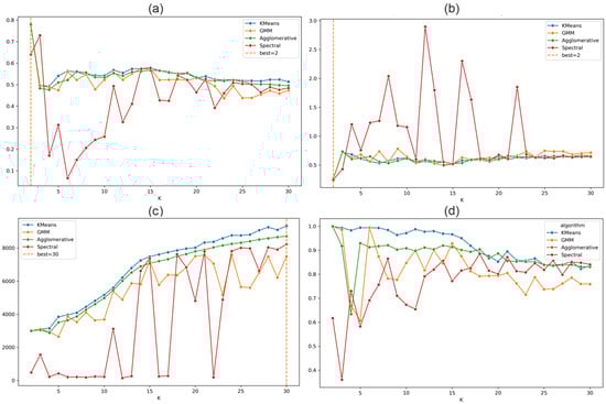
Figure 10. Evaluation metrics for the clustering results for the complete feature vector (Tokachi-oki case). The dashed line marks the optimal number of clusters (K). (a) Silhouette coefficient; (b) Davies–Bouldin index; (c) Calinski–Harabasz index; and (d) stability analysis using the Adjusted Rand Index (ARI).

To assess the cross-algorithm stability and determine the optimal number of clusters, we computed the pairwise ARI heatmap (Figure S7) and the ${\overline{ARI}}_{alg}(K)$ metric (Figure 11). The resulting ARI heatmap indicate the most consistent partitions at K = 14–16, indicating a stable structure in this area. The ${\overline{ARI}}_{alg}(K)$ values show a clear maximum at K = 15 reaching approximately 0.92. This suggests that clustering solutions with 15 clusters are the most consistent across repeated runs and thus represent the most robust structure in the data. For smaller K < 15 or larger K > 15 numbers of clusters, ${\overline{ARI}}_{alg}(K)$ values decrease, indicating less stable or over-fragmented partitions. Overall, the ARI-based stability assessment supports selecting K = 15 as the optimal number of clusters, capturing a more refined segmentation of the deformation field influenced by the Tokachi-oki earthquake-related processes.

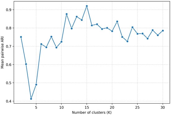
Figure 11. Results of ARI-based estimation of the optimal number of clusters for the complete feature vector (Tokachi-oki case).

We performed clustering using all K-based algorithms (Kmeans, GMM, HAC and SPC), adopting the optimal values of $K_{opt}^F$ = 15 to derive the possible tectonic segmentation of the Japanese Islands. Clustering solutions in the UMAP-reduced space are shown in Figure S8 and on the geographic map in Figure S9. The results from all four clustering K-based techniques are highly consistent in the UMAP-reduced space for $K_{opt}^F$ = 15, in agreement with the high values of ${\overline{ARI}}_{alg}(K)$ metric.

To further validate our results, we performed independent clustering using the modern HDBSCAN method. Iterative tuning of HDBSCAN hyperparameters for the two-feature vector case (Table 6) explored a range of minimum cluster sizes and minimum samples to optimize cluster stability and minimize noise points. The tuning indicated that a minimum cluster size of 15–20 and a minimum samples value of 10 provide the most robust clustering, capturing the main data structures while keeping the fraction of unassigned points below 14%. HDBSCAN identified an optimum of K = 14 clusters very similar to the previously determined $K_{opt}^F$ = 15. We assume that K = 14–15 is therefore the most reliable estimate of clearly distinguished clusters in the Japanese Islands base on the full feature vector for Tokachi-oki.

Table 6. Results of iterative tuning of HDBSCAN parameter for the complete feature vector (Tokachi-oki case).

Minimum Cluster Size	Minimum of Samples	Noise, %	Silhouette Index	Number of Clusters
15	10	13.54	0.632786	14
20	10	13.43	0.632786	13
5	10	13.89	0.596488	19
10	10	13.89	0.596488	19
5	5	17.82	0.593585	35
20	5	9.14	0.588542	15
15	5	9.72	0.579341	16
30	1	6.37	0.569264	13
10	5	10.07	0.560099	21
20	1	5.21	0.556993	16
15	1	6.48	0.530774	20
5	1	11.57	0.514690	72
10	1	9.38	0.495977	34
30	10	3.13	0.435302	8
30	5	0.69	0.422177	8

A comparison between the consensus solution and the HDBSCAN results reveals a moderate to high degree of agreement in both the UMAP-reduced feature space (Figure 12) and in the geographic domain (Figure 13). The primary differences arise in sparsely populated regions associated with unstable or transitional deformation regimes, which HDBSCAN classifies as noise. This ability to explicitly identify noise while preserving the stable cluster structure underscores an important advantage of HDBSCAN for analyzing GNSS data affected by variable signal quality and nonstationary deformation behavior.

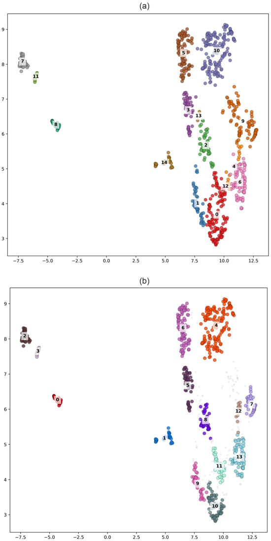
Figure 12. Clustering solutions in the UMAP-reduced space for the complete feature vector (Tokachi-oki case). Number of clusters is set to 15 for Consensus and 14 for HDBSCAN. Panels show results from (a) Consensus clustering, (b) HDBSCAN.

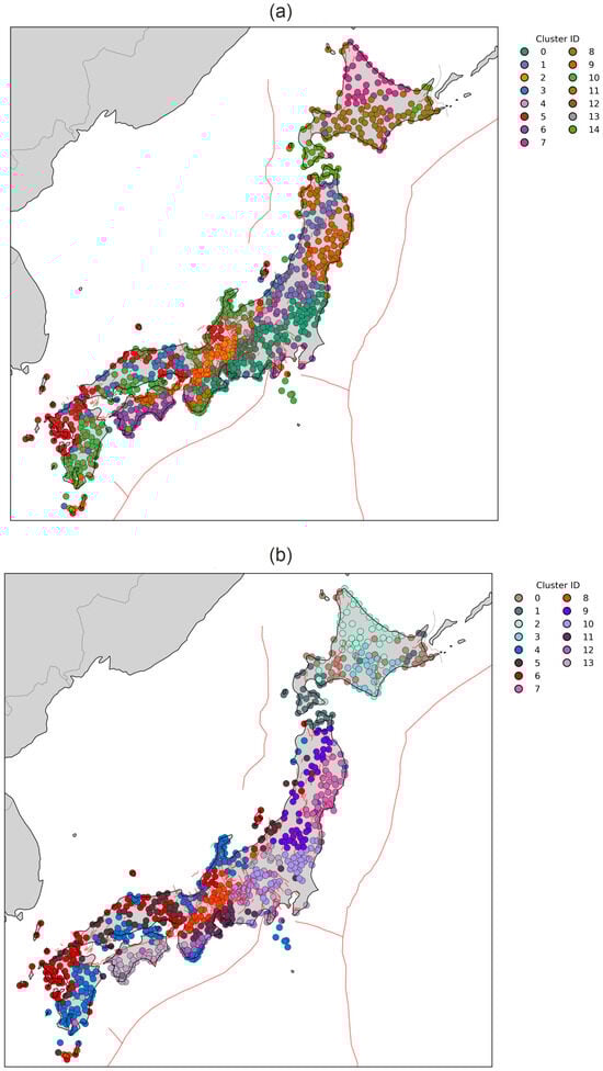
Figure 13. Geographic distribution of clustering results obtained for the complete feature vector (Tokachi-oki case). Number of clusters is set to 15 for consensus and 14 for HDBSCAN. Panels show results from (a) Consensus clustering, (b) HDBSCAN.

In contrast to the steady-state velocity field, which yields four large-scale clusters that primarily delineate Japan’s first-order tectonic architecture—including clear segmentation along the MTL, the ISTL, and trench-parallel belts reflecting steady-state strain-accumulation gradients—the Tokachi-oki-specific feature vector produces a finer segmentation of the deformation field. Using the full Tokachi-oki feature set, which incorporates co-seismic and post-seismic transient offsets, consensus clustering resolves 15 spatially coherent clusters (Figure 13a). These clusters capture a substantially more complex deformation pattern, revealing localized variations that are not detectable in the velocity-only analysis.

First, northern Honshu and Hokkaido exhibit strong internal differentiation, reflecting spatially variable post-seismic relaxation and fault-controlled kinematic domains associated with the 2003 Tokachi-oki earthquake. Second, along the Pacific margin, numerous narrow, trench-parallel clusters emerge, indicating that transient deformation enhances along-arc segmentation beyond what is visible in the steady velocity field. Third, central Honshu shows a patchwork of small clusters that coincide with the Fossa Magna.

The HDBSCAN solution (Figure 13b) provides a complementary perspective, emphasizing the most persistent and density-supported structures in the Tokachi-oki feature space. While the number of clusters is similar (14 in the HDBSCAN case), HDBSCAN sharpens the segmentation by removing low-confidence assignments and capturing compact, high-density domains. Notably, HDBSCAN highlights strong subdivision in eastern Hokkaido, multiple sub-domains along the fore-arc of northern Honshu, and enhanced segmentation across the MTL and other major crustal boundaries.

Overall, the Tokachi-oki feature vector reveals a much richer tectonic segmentation than the steady-state velocity field alone. This demonstrates that transient GNSS signals—especially those associated with large offshore earthquakes—add substantial discriminatory power to clustering, exposing short-term deformation domains that are otherwise hidden within long-term velocity gradients.

4.3. Clustering of the Complete Feature Vector for the Tohoku Case

In the final stage of our clustering analysis, we examined the segmentation obtained from the full feature vector, which includes both strain-rate and offset-related features associated with the 2011 Tohoku earthquake (Figure 3). This Mw 9.0 event occurred offshore along the Pacific coast of northern Honshu. Despite its relatively compact source geometry, the earthquake produced strain-accumulation and co-seismic–post-seismic deformation signals that extend across nearly all of the Japanese Islands. (Figure 1).

The SC (Figure 14a) and DBI (Figure 14b) validity metrics both marks $K$ = 3–5 as an optimal number of clusters. This is consistent with the assumption about coherent deformation of continental margin during a stable inter-seismic stage of the seismic cycle. Nevertheless, the CHI maximizes only at K = 29, indicating the presence of possible fine structure in GNSS data (Figure 14c). The $\overline{ARI}(K)$ stability index (Figure 14d) shows less consistency than in the two-feature case, reaching relatively high values (>0.8) for K = 2–20 (for K-based algorithms), further supporting the notion of potential multi-scale segmentation in the full feature space.

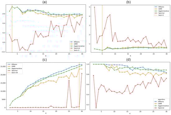
Figure 14. Evaluation metrics for the clustering results for the complete feature vector (Tohoku case). The dashed line marks the optimal number of clusters (K). (a) Silhouette coefficient; (b) Davies–Bouldin index; (c) Calinski–Harabasz index; and (d) stability analysis using the Adjusted Rand Index (ARI).

To assess the cross-algorithm stability and determine the optimal number of clusters, we computed the pairwise ARI heatmap (Figure S12) and the ${\overline{ARI}}_{alg}(K)$ metric (Figure 15). The resulting ARI heatmap indicate consistent partitions at K = 4–6 and K > 17, indicating stable structures in these areas. The ${\overline{ARI}}_{alg}(K)$ values show clear maximums at K = 5, K = 18, K = 25 and K = 30, reaching approximately 0.71–0.78. This suggests that clustering solutions with 5,18, 25 and 30 clusters are the most consistent across repeated runs and thus represent the most robust structure in the data. For smaller K < 5 numbers of clusters, ${\overline{ARI}}_{alg}(K)$ values decrease, indicating less stable partitions. Overall, the ARI-based stability assessment supports selecting K = 5, 18, 25 and 30 provide optimal cluster numbers, reflecting both the coarse segmentation and progressively finer hierarchical structures in the deformation field associated with Tohoku earthquake-related processes.

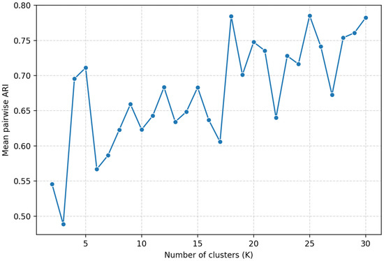
Figure 15. Results of ARI-based estimation of the optimal number of clusters for the complete feature vector (Tohoku case).

We performed clustering using all K-based algorithms (Kmeans, GMM, HAC and SPC), adopting the optimal values of $K_{opt}^F$ = 5 and $K_{opt}^F$ = 18 to derive the possible tectonic segmentation of the Japanese Islands. Clustering solutions in the UMAP-reduced space are shown in Figures S13 and S15 and on the geographic map in Figures S14 and S16. The results from all four clustering K-based techniques are highly consistent in the UMAP-reduced space for $K_{opt}^F$ = 5, in agreement with the high values of ${\overline{ARI}}_{alg}(K)$ metric. For $K_{opt}^F$ = 18 some differences emerge, reflecting alternative ways of subdividing the initial clusters.

To further validate our results, we performed independent clustering using the modern HDBSCAN method. Iterative tuning of HDBSCAN hyperparameters for the two-feature vector case (Table 7) explored a range of minimum cluster sizes and minimum samples to optimize cluster stability and minimize noise points. The tuning indicated that a minimum cluster size of 5–10 and a minimum samples value of 10 provide the most robust clustering, capturing the main data structures while keeping the fraction of unassigned points below 12%. The alternative set of hyperparameters (minimum cluster size = 20, minimum samples = 5) produces a similar Silhouette Score while generating even less noise (<8%). Thus, HDBSCAN identified an optimum of K = 15 and K = 22 clusters similar to the previously determined $K_{opt}^F$ = 18. We assume that K = 15–22 is therefore the most reliable estimate of clearly distinguished clusters in the Japanese Islands base on the full feature vector for Tohoku.

Table 7. Results of iterative tuning of HDBSCAN parameter for the complete feature vector (Tohoku case).

Minimum Cluster Size	Minimum of Samples	Noise, %	Silhouette Index	Number of Clusters
5	10	12.04	0.709692	22
10	10	12.04	0.709692	22
20	5	7.75	0.705100	15
15	5	8.68	0.682760	19
30	1	4.86	0.675231	14
5	5	7.52	0.671453	32
10	5	8.10	0.670623	25
30	5	2.66	0.668798	13
20	1	8.45	0.652204	17
15	1	3.13	0.652111	20
10	1	4.75	0.632783	27
20	10	0.81	0.614077	10
30	10	0.81	0.614077	10
15	10	1.85	0.605961	13
5	1	12.96	0.578300	68

The clustering results for solutions with fewer clusters (K = 5 for consensus clustering and K = 15 for HDBSCAN) show clear grouping in the UMAP-reduced feature space (Figure 16). The consensus clustering solution for K = 5 (Figure 17a) closely resembles the velocity-only clustering outcome (Figure 9), representing a coarse segmentation of the Japanese Islands, but with clearer separation between strongly affected near-trench stations in Tohoku, the resilient back-arc domain, and southwestern Japan. The inclusion of co-seismic and post-seismic terms introduces a distinct Tohoku source zone cluster that was less explicit in the steady-state velocity results. Comparison between the consensus solution and the HDBSCAN results for a larger number of clusters reveals a moderate to high level of agreement, both in the UMAP-reduced feature space (Figure 18) and in the geographic domain (Figure 19). The main differences appear in sparsely populated regions associated with unstable or transitional deformation regimes, which HDBSCAN identifies as noise and produces slightly different numbers of clusters. The ability of HDBSCAN to explicitly detect noise while preserving stable cluster structures highlights its advantage for analyzing GNSS data affected by variable signal quality and nonstationary deformation behavior. Consensus clustering results for K = 18 (Figure 19a) further subdivides Japanese Islands hierarchically, resolving fine-scale segmentation within Tohoku and Hokkaido, and distinguishing localized zones of elevated post-seismic response. In contrast, HDBSCAN applied to the same feature set (Figure 19b) produces a more irregular but spatially precise mapping, detecting small, high-density deformation domains along the Pacific coast and several isolated microclusters associated with strong co-seismic displacement. The consensus solution remains smoother and structurally coherent, whereas HDBSCAN highlights localized complexity and transient deformation heterogeneity.

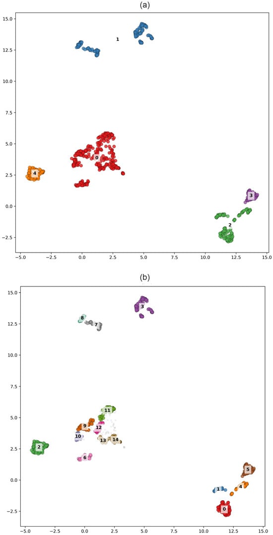
Figure 16. Clustering solutions in the UMAP-reduced space for the complete feature vector (Tohoku case). Number of clusters is set to 5 for Consensus and 15 for HDBSCAN. Panels show results from (a) Consensus clustering, (b) HDBSCAN.

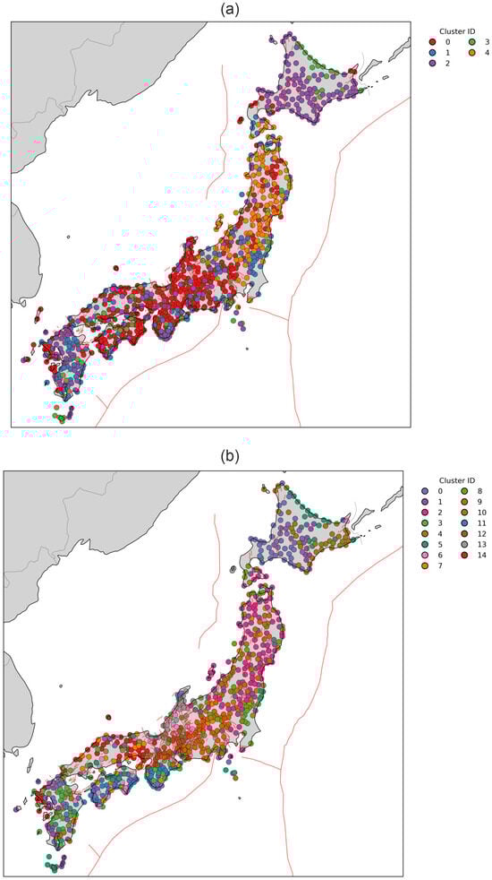
Figure 17. Geographic distribution of clustering results obtained for the complete feature vector (Tohoku case). Number of clusters is set to 5 for consensus and 15 for HDBSCAN. Panels show results from (a) Consensus clustering, (b) HDBSCAN.

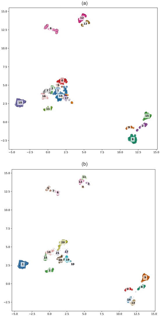
Figure 18. Clustering solutions in the UMAP-reduced space for the complete feature vector (Tohoku case). Number of clusters is set to 18 for Consensus and 22 for HDBSCAN. Panels show results from (a) Consensus clustering, (b) HDBSCAN.

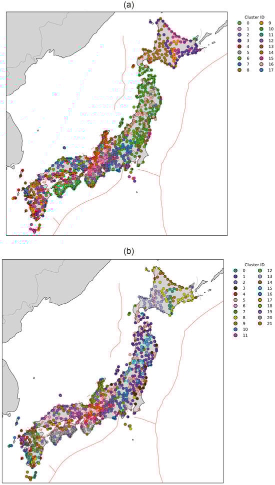
Figure 19. Geographic distribution of clustering results obtained for the complete feature vector (Tohoku case). Number of clusters is set to 18 for consensus and 22 for HDBSCAN. Panels show results from (a) Consensus clustering, (b) HDBSCAN.

4.4. Comparison of Clustering Results

To evaluate the consistency between obtained clustering solutions and highlight regions sensitive to feature selection, we computed ΔC fields representing pointwise differences between cluster labels obtained from alternative feature sets. Figure 20 illustrates ΔC for two consensus clustering configurations: Tohoku–Tokachi ΔC, comparing clustering results based on earthquake-specific feature vectors, and Tohoku–VEL2 ΔC, comparing results based on Tohoku-related features with the velocity-only clustering.

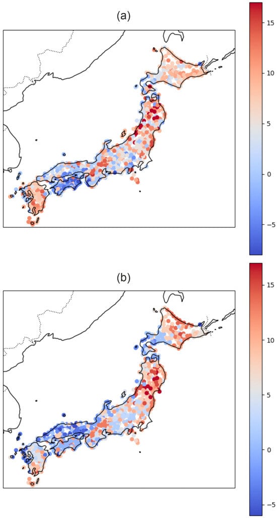
Figure 20. Geographic distribution of ΔC results obtained for (a) the difference between the two-feature vector consensus clustering and Tohoku complete feature vector consensus clustering, (b) the difference between the Tohoku and Tokachi-oki complete feature vectors.

The spatial distribution of the ΔC values (Figure 20a) reveals systematic differences between the consensus clustering obtained for the full Tohoku dataset and the clustering derived from velocity-only (VEL2) features. Positive ΔC values (warm colors) indicate stations assigned to higher-indexed clusters in the Tohoku solution relative to the VEL2 solution, whereas negative values (cool colors) mark stations that shift toward lower-indexed clusters.

Overall, the pattern highlights several coherent tectonic domains where the inclusion of additional deformation-related features substantially modifies the clustering structure. Along the Pacific side of northeastern Honshu, broad regions of positive ΔC dominate, indicating that the Tohoku solution tends to group these stations into more dynamically active or internally heterogeneous clusters than the velocity-only analysis suggests. In contrast, southwestern Japan (Shikoku and Kyushu) exhibits extensive negative ΔC values, implying that when full time-series-derived features are incorporated, these areas converge toward more uniform cluster assignments relative to the velocity-only case. The transition zones between these domains, especially along central Honshu, show a fine-scale mosaic of positive and negative ΔC, reflecting localized sensitivities to non-velocity features such as episodic offsets or transient deformation signals.

The spatial distribution of ΔC values shown on Figure 20b reveals systematic, tectonically meaningful differences between the Tokachi- and Tohoku-based clusterings. Positive ΔC values dominate along the Pacific margin of northeast Honshu and Hokkaido, particularly in the Sanriku–Tohoku forearc, where stations are reassigned to higher-index clusters in the Tohoku-based solution. This indicates that the Tohoku-derived feature set emphasizes stronger deformation signatures and greater structural complexity in the forearc domain. A pronounced positive anomaly extends from Fukushima through Miyagi to Iwate, consistent with enhanced strain gradients and post-seismic effects associated with the 2011 Tohoku earthquake.

In contrast, negative ΔC values cluster across southwest Honshu, Shikoku, and parts of western Hokkaido, suggesting that Tokachi-based features classify these regions into comparatively higher-complexity clusters, while the Tohoku-based features assign them to more homogeneous, lower-index groups. These negative values reflect regional deformation patterns that are more sensitive to the 2003 Tokachi-oki event than to the Tohoku sequence.

Regions with ΔC ≈ 0—including central Honshu and parts of northern Hokkaido—correspond to stable domain assignments across both earthquake scenarios, indicating consistent structural behavior and relatively uniform deformation rates. Overall, the ΔC field highlights coherent, large-scale reorganization of cluster boundaries between the two feature sets and delineates zones of strong sensitivity to event-specific deformation manifolds.

Both Δ-maps reveal coherent spatial patterns of cluster disagreement. The largest ΔC values are concentrated along the Pacific margin of Honshu and Hokkaido—areas strongly affected by the 2003 Tokachi-oki and the 2011 Tohoku earthquakes—indicating that inclusion of transient seismic features significantly alters tectonic grouping. In contrast, southwestern Japan and the back-arc region display lower ΔC, implying stable classification largely independent of feature choice. Overall, the Δ-clustering approach provides a quantitative measure of sensitivity in cluster assignments and helps identify zones where seismic transients play a dominant role in deformation behavior.

5. Discussion

Active continental margins, such as Japanese Islands, are complex geodynamic systems where lithospheric deformation results from interactions among tectonic blocks separated by faults with varying strength and permeability. Due to the strong rheological contrast between blocks and faults, such systems may respond to loading either as a quasi-continuous medium or as a set of weakly coupled elements capable of relative motion and rotation. This dual behavior becomes especially evident across different stages of the seismic cycle. Additionally, the surface velocity field in Japan is strongly influenced by subduction-driven 3D deformation, unlike mainly strike-slip regions such as California. As a result, GNSS-based clustering in Japan reflects a combination of block-related motions and strain accumulation/release anomalies.

In this study, we adopt a hard clustering approach to identify compact clusters in the feature space associated with the kinematics and deformation of tectonic blocks. Tectonic blocks are spatially compact, typically convex, and exhibit well-defined boundaries; therefore, GNSS stations are assigned strictly to a single cluster. Our approach extends traditional feature vectors by incorporating parameters associated with time-dependent crustal deformation and combines standard clustering algorithms with internal validity metrics to achieve stable segmentations.

Unlike deep learning approaches such as autoencoders, recurrent networks, or data-driven trajectory encoders, which extract latent representations based solely on statistical patterns, our method constructs features that are explicitly tied to the physics of the seismic cycle. The regression basis is designed a priori to represent well-understood tectonic processes: secular plate motion, periodic environmental loading, co-seismic offsets, and post-seismic relaxation. As a result, each regression coefficient has a direct geophysical interpretation rather than being an abstract latent variable. This interpretability is essential for studying crustal block behavior, because it ensures that spatial patterns identified through clustering reflect genuine differences in tectonic loading and rheology rather than opaque statistical structures learned by a model. Our physically informed feature extraction therefore provides a transparent alternative to deep learning, enabling meaningful comparisons across stations and improving the reliability of geodynamic inferences. Nevertheless, in our future work we are planning to extend the approach by using more specific clustering algorithms, validity metrics and linkage approaches.

Several previously published articles support the complex tectonic segmentation of the Japanese Islands accommodating the compression strain due to subduction [4,8,10,11,12,13,15,22]. The results of our study are consistent with these models in identifying main tectonic patterns of Japanese Islands: large blocks in the northeastern part of Honshu Island, complex tectonic structure in Fossa Magna, fragmentation of Kyushu, Shikoku and southwestern part of Honshu Islands on smaller blocks associated with the Median Tectonic Line.

Our clustering results indicate that, in the context of long-term deformation, the tectonic blocks previously identified in seismotectonic and block-motion studies deform largely coherently during the accumulation of inter-seismic strain caused by subduction of the oceanic plates. The detected anomalies in the deformation field correspond to the principal tectonic structures of the Japanese Islands—such as the Fossa Magna, the Median Tectonic Line, and regions undergoing preparation for megathrust earthquakes.

We constructed feature vectors combining steady-state and time-dependent deformation parameters. Future work will explore clustering based on direct year-to-year GNSS variations and implement advanced clustering approaches, including density-based, graph-based, and spatiotemporal methods, to further refine tectonic segmentation.

6. Conclusions

Our work demonstrates the power of combining machine learning methods and time-dependent characteristics of the deformation field to better understand strain and rotation patterns in subduction margins and their interplay with geological structures and long-term tectonic domains. We analyzed 20 years of continuous GNSS observations from the Japanese Islands to identify spatiotemporal deformation domains corresponding to independent tectonic block motions or zones of anomalous deformation associated with the preparation of large megathrust earthquakes.

We developed a novel clustering methodology that extends the traditional feature vector describing GNSS station kinematics with regression-derived parameters capturing temporal variations in surface strain. This approach allows us to account for spatial heterogeneities in the GNSS network and temporal evolution of elastic stress accumulation and relaxation. We demonstrated that a carefully designed feature-generation workflow—incorporating robust outlier detection, feature-distribution characterization, and feature-specific scaling—helps preserve stable clustering outcomes even when using an expanded feature vector in a noisy deformation environment. By combining multiple clustering algorithms and internal validity metrics, our method achieves stable and interpretable segmentation of deformation domains. Modern clustering methods such as HDBSCAN demonstrate clear advantages for analyzing GNSS data affected by variable signal quality and nonstationary deformation behavior, owing to their ability to explicitly identify noise while simultaneously preserving the underlying stable cluster structure.

Our results highlight several key contributions:

• A physically interpretable feature construction framework for GNSS time series can capture key tectonic processes.
• A clustering workflow integrating multiple unsupervised algorithms and stability metrics that robustly identifies tectonic blocks.
• A generalizable methodology that can be applied to other active regions with dense GNSS networks and poorly constrained tectonic structures.

Overall, this study offers new insights into crustal fragmentation, provides a robust approach for identifying spatiotemporal deformation domains, and contributes data valuable for improving seismic hazard assessment and refining models of strain accumulation and release in tectonically active regions.

References

- Argus, D.F.; Gordon, R.G.; DeMets, C. Geologically current motion of 56 plates relative to the no-net-rotation reference frame. Geochem. Geophys. Geosyst. 2011, 12, Q11001. [Google Scholar] [CrossRef]
- Barnhart, W.; Chaussard, E. The Seismic Cycle: From Observations to Models of Fault Slip. In Remote Sensing for Characterization of Geohazards and Natural Resources; Chaussard, E., Jones, C., Chen, J.A., Donnellan, A., Eds.; Springer Remote Sensing/Photogrammetry; Springer: Cham, Switzerland, 2024. [Google Scholar] [CrossRef]
- Scholz, C.H. The Mechanics of Earthquakes and Faulting, 2nd ed.; Cambridge University Press: Cambridge, UK; New York, NY, USA; Melbourne, Australia, 2019; 516p. [Google Scholar] [CrossRef]
- Loveless, J.P.; Meade, B.J. Geodetic imaging of plate motions, slip rates, and partitioning of deformation in Japan. J. Geophys. Res. 2010, 115, B02410. [Google Scholar] [CrossRef]
- Panayotopoulos, Y.; Hirata, N.; Sato, H.; Kato, A.; Imanishi, K.; Kuwahara, Y.; Cho, I.; Takeda, T.; Asano, Y. Investigating the role of the Itoigawa-Shizuoka tectonic line towards the evolution of the Northern Fossa Magna rift basin. Tectonophysics 2014, 615, 12–26. [Google Scholar] [CrossRef]
- Ozawa, S.; Nishimura, T.; Suito, H.; Kobayashi, T.; Tobita, M.; Imakiire, T. Coseismic and postseismic slip of the 2011 magnitude-9 Tohoku-Oki earthquake. Nature 2011, 475, 373–376. [Google Scholar] [CrossRef]
- Pollitz, F.F. Gravitational viscoelastic postseismic relaxation on a layered spherical Earth. J. Geophys. Res. 1997, 102, 17921–17941. [Google Scholar] [CrossRef]
- Hashimoto, M.; Miyazaki, S.; Jackson, D.D. A block-fault model for deformation of the Japanese Islands derived from continuous GPS observation. Earth Planet Sp. 2000, 52, 1095–1100. [Google Scholar] [CrossRef]
- Nishimura, T.; Sagiya, T.; Stein, R.S. Crustal block kinematics and seismic potential of the northernmost Philippine Sea plate and Izu microplate, central Japan, inferred from GPS and leveling data. J. Geophys. Res. 2007, 112, B05414. [Google Scholar] [CrossRef]
- Nishimura, T.; Yokota, Y.; Tadokoro, K.; Ochi, T. Strain partitioning and interplate coupling along the northern margin of the Philippine Sea plate, estimated from Global Navigation Satellite System and Global Positioning System-Acoustic data. Geosphere 2018, 14, 535–551. [Google Scholar] [CrossRef]
- Kimura, H.; Tadokoro, K.; Ito, T. Interplate coupling distribution along the Nankai Trough in southwest Japan estimated from the block motion model based on onshore GNSS and seafloor GNSS/A observations. J. Geophys, Res. Solid Earth 2019, 124, 6140–6164. [Google Scholar] [CrossRef]
- Tanaka, Y.; Kano, M.; Nishimura, T.; Ohta, Y.; Yano, K. Numerical experiment toward simultaneous estimation of the spatiotemporal evolution of interseismic fault slips and block motions in southwest Japan. Earth Planets Space 2024, 76, 69. [Google Scholar] [CrossRef]
- Kawabata, H.; Yoshioka, S. Spatiotemporal changes in the strain field in the Niigata–Kobe Tectonic Zone: Long-term analysis using GNSS time series data. Prog. Earth Planet. Sci. 2025, 12, 22. [Google Scholar] [CrossRef]
- Savage, J.C. Euler-vector clustering of GPS velocities defines microplate geometry in southwest Japan. J. Geophys. Res. Solid Earth 2018, 123, 1954–1968. [Google Scholar] [CrossRef]
- Qu, W.; Wang, J.; Yang, Y.; Gao, Y.; Li, J.; Wang, Y.; Zhang, Q.; Hao, M. Fine divided method of active tectonic blocks based on adaptive density peak clustering and improved Euler model, revealed by GNSS velocities in Southwest Japan. Tectonophysics 2022, 844, 229635. [Google Scholar] [CrossRef]
- Kubo, H.; Naoi, M.; Kano, M. Recent advances in earthquake seismology using machine learning. Earth Planets Space 2024, 76, 36. [Google Scholar] [CrossRef]
- Kılıç, B.; Özarpacı, S. Ensemble Clustering in GPS Velocities: A Case Study of Turkey. Appl. Sci. 2022, 12, 12636. [Google Scholar] [CrossRef]
- Takahashi, A.; Hashimoto, M. Cluster analysis of dense GNSS velocity field reveals characteristics associated with regional tectonics in New Zealand. J. Geophys. Res. Solid Earth 2022, 127, e2022JB024793. [Google Scholar] [CrossRef]
- Takahashi, A.; Yano, K.; Kano, M. A GNSS-velocity clustering method applicable at local to global scales. J. Geophys. Res. Solid Earth 2025, 130, e2024JB029689. [Google Scholar] [CrossRef]
- Şafak Yaşar, Ş.; Tiryakioğlu, İ.; Aktuğ, B.; Erdoğan, H.; Özkaymak, Ç. Determination of Anatolian Plate’s tectonic block boundaries with clustering analysis using GNSS sites velocities. Geomat. Nat. Hazards Risk 2025, 16, 2446588. [Google Scholar] [CrossRef]
- Simpson, R.W.; Thatcher, W.; Savage, J.C. Using cluster analysis to organize and explore regional GPS velocities. Geophys. Res. Lett. 2012, 39, L18307. [Google Scholar] [CrossRef]
- Savage, J.C.; Simpson, R.W. Clustering of GPS velocities in the Mojave Block, southeastern California. J. Geophys. Res. 2013, 118, 1747–1759. [Google Scholar] [CrossRef]
- Yáñez-Cuadra, V.; Moreno, M.; Ortega-Culaciati, F.; Donoso, F.; Báez, J.C.; Tassara, A. Mosaicking Andean morphostructure and seismic cycle crustal deformation patterns using GNSS velocities and machine learning. Front. Earth Sci. 2023, 11, 1096238. [Google Scholar] [CrossRef]
- Granat, R.; Donnellan, A.; Heflin, M.; Lyzenga, G.; Glasscoe, M.; Parker, J.; Pierce, M.; Wang, J.; Rundle, J.; Ludwig, L.G. Clustering Analysis Methods for GNSS Observations: A Data-Driven Approach to Identifying California’s Major Faults. Earth Space Sci. 2021, 8, e2021EA001680. [Google Scholar] [CrossRef]
- Ester, M.; Kriegel, H.-P.; Sander, J.; Xu, X. A Density-Based Algorithm for Discovering Clusters in Large Spatial Databases with Noise; AAAI Press: Washington, DC, USA, 1996; pp. 226–231. [Google Scholar]
- Campello, R.J.G.B.; Moulavi, D.; Sander, J. Density-Based Clustering Based on Hierarchical Density Estimates. In Advances in Knowledge Discovery and Data Mining; Pei, J., Tseng, V.S., Cao, L., Motoda, H., Xu, G., Eds.; Springer: Berlin/Heidelberg, Germany, 2013. [Google Scholar] [CrossRef]
- Ng, A.Y.; Jordan, M.I.; Weiss, Y. On spectral clustering: Analysis and an algorithm. In Advances in Neural Information Processing Systems, 14; Dietterich, T.G., Becker, S., Ghahramani, Z., Eds.; MIT Press: Cambridge, MA, USA, 2002. [Google Scholar]
- Shi, J.; Malik, J. Normalized cuts and image segmentation. IEEE Trans. Pattern Anal. Mach. Intell. 2000, 22, 888–905. [Google Scholar] [CrossRef]
- von Luxburg, U. A tutorial on spectral clustering. Stat. Comput. 2007, 17, 395–416. [Google Scholar] [CrossRef]
- Kumar, U.; Legendre, C.P.; Lee, J.C.; Zhao, L.; Chao, B.F. On analyzing GNSS displacement field variability of Taiwan: Hierarchical Agglomerative Clustering based on Dynamic Time Warping technique. Comput. Geosci. 2022, 169, 105243. [Google Scholar] [CrossRef]
- Paparrizos, J.; Gravano, L. K-Shape: Efficient and Accurate Clustering of Time Series. In Proceedings of the 2015 ACM SIGMOD International Conference on Management of Data, Melbourne, VIC, Australia, 31 May–4 June 2015; Association for Computing Machinery: New York, NY, USA, 2015; pp. 1855–1870. [Google Scholar] [CrossRef]
- Patara, T.; Shin, Y.; Kang, J.; Nam, Y.; Na, J.; Bae, M.; Kim, J.; Kim, B.; Lee, J.-G. Universal Time-Series Representation Learning: A Survey. arXiv 2024. [Google Scholar] [CrossRef]
- DeMets, C.; Gordon, R.G.; Argus, D.F.; Stein, S. Effect of Recent Revisions to the Geomagnetic Reversal Time Scale on Estimates of Current Plate Motions. Geophys. Res. Lett. 1994, 21, 2191–2194. [Google Scholar] [CrossRef]
- Styron, R.; Pagani, M. The GEM Global Active Faults Database. Earthq. Spectra 2020, 36, 160–180. [Google Scholar] [CrossRef]
- International Seismological Centre. Online Bulletin. Available online: https://www.isc.ac.uk/iscbulletin/search/ (accessed on 14 December 2025).
- Dziewonski, A.M.; Chou, T.-A.; Woodhouse, J.H. Determination of earthquake source parameters from waveform data for studies of global and regional seismicity. J. Geophys. Res. 1981, 86, 2825–2852. [Google Scholar] [CrossRef]
- Ekström, G.; Nettles, M.; Dziewonski, A.M. The global CMT project 2004-2010: Centroid-moment tensors for 13,017 earthquakes. Phys. Earth Planet. Inter. 2012, 200–201, 1–9. [Google Scholar] [CrossRef]
- Lobkovsky, L.I.; Kerchman, V.I.; Baranov, B.V.; Pristavakina, E.I. Analysis of seismotectonic processes in subduction zones from the standpoint of a keyboard model of great earthquakes. Tectonophysics 1991, 199, 211–236. [Google Scholar] [CrossRef]
- GSI Website. Available online: https://www.gsi.go.jp/ENGLISH/geonet_english.html (accessed on 12 November 2025).
- McInnes, L.; Healy, J. UMAP: Uniform Manifold Approximation and Projection for Dimension Reduction. arXiv 2018. [Google Scholar] [CrossRef]
- Mojena, R. Hierarchical grouping methods and stopping rules: An evaluation. Comput. J. 1977, 20, 359–363. [Google Scholar] [CrossRef]
- Hartigan, J.A.; Wong, M.A. Algorithm AS 136: A k-means clustering algorithm. J. R. Stat. Soc. Ser. C Appl. Stat. 1979, 28, 100–108. [Google Scholar] [CrossRef]
- Reynolds, D. Gaussian Mixture Models. In Encyclopedia of Biometrics; Li, S.Z., Jain, A., Eds.; Springer: Boston, MA, USA, 2009. [Google Scholar] [CrossRef]
- Arbelaitz, O.; Gurrutxaga, I.; Muguerza, J.; Pérez, J.M.; Perona, I. An extensive comparative study of cluster validity indices. Pattern Recognit. 2013, 46, 243–256. [Google Scholar] [CrossRef]
- Rousseeuw, P.J. Silhouettes: A graphical aid to the interpretation and validation of cluster analysis. J. Comput. Appl. Math. 1987, 20, 53–65. [Google Scholar] [CrossRef]
- Davies, D.L.; Bouldin, D.W. A Cluster Separation Measure. IEEE Trans. Pattern Anal. Mach. Intell. 1979, PAMI-1, 224–227. [Google Scholar] [CrossRef]
- Caliński, T.; Harabasz, J. A dendrite method for cluster analysis. Commun. Stat. 1974, 3, 1–27. [Google Scholar] [CrossRef]
- Hubert, L.; Arabie, P. Comparing partitions. J. Classif. 1985, 2, 193–218. [Google Scholar] [CrossRef]
- Rand, W.M. Objective criteria for the evaluation of clustering methods. J. Am. Stat. Assoc. 1971, 66, 846–850. [Google Scholar] [CrossRef]
- Monti, S.; Tamayo, P.; Mesirov, J.; Golub, T. Consensus Clustering: A Resampling-Based Method for Class Discovery and Visualization of Gene Expression Microarray Data. Mach. Learn. 2003, 52, 91–118. [Google Scholar] [CrossRef]
- Nguyen, N.; Caruana, R. Consensus Clusterings. In Proceedings of the Seventh IEEE International Conference on Data Mining (ICDM 2007), Omaha, NE, USA, 28–31 October 2007; pp. 607–612. [Google Scholar] [CrossRef]
- Gabsatarov, Y.V.; Vladimirova, I.S. Machine learning for GNSS time series analysis in the time domain. Russ. J. Earth Sci. 2025, 25. [Google Scholar] [CrossRef]
- Blewitt, G.; Kreemer, C.; Hammond, W.C.; Gazeaux, J. MIDAS robust trend estimator for accurate GPS station velocities without step detection. J. Geophys. Res. Solid Earth 2016, 121, 2054–2068. [Google Scholar] [CrossRef]
- Truong, C.; Oudre, L.; Vayatis, N. Selective review of offline change point detection methods. Signal Process. 2020, 167, 107299. [Google Scholar] [CrossRef]
- Fritsch, F.N.; Carlson, R.E. Monotone Piecewise Cubic Interpolation. SIAM J. Numer. Anal. 1980, 17, 238–246. [Google Scholar] [CrossRef]
- Shen, Z.-K.; Jackson, D.D.; Ge, B.X. Crustal deformation across and beyond the Los Angeles basin from geodetic measurements. J. Geophys. Res. 1996, 101, 27957–27980. [Google Scholar] [CrossRef]
Disclaimer/Publisher’s Note: The statements, opinions and data contained in all publications are solely those of the individual author(s) and contributor(s) and not of MDPI and/or the editor(s). MDPI and/or the editor(s) disclaim responsibility for any injury to people or property resulting from any ideas, methods, instructions or products referred to in the content. |
© 2025 by the authors. Licensee MDPI, Basel, Switzerland. This article is an open access article distributed under the terms and conditions of the Creative Commons Attribution (CC BY) license.