Abstract
Sampling with replacement occurs when drawing without removing individuals from finite populations. It is a common distribution technique used in physics, biology, and medicine. It is used in state analysis of qubits, the physics of particle interactions, studies of genetic variation and variability, and analyzing the treatment effects from clinical trial analyses. When applied, sample statistics should be accompanied by confidence intervals. The major difficulty in expressing the confidence intervals in sampling with replacement consists of discreetness regarding the probability distribution. As a result, no mathematical formula can handle an optimum solution. Using a simple algorithm is proposed in order to obtain confidence intervals for sampling with replacement variables (x from m trials with replacement) and their proportion (). A question-based discussion is presented. Traditional confidence intervals often require large sample sizes. Confidence intervals, constructed in a deterministic way provided by the proposed algorithm for sampling with replacement, allow constructing intervals without constraints.
1. Introduction
The sampling strategy is foundational when dealing with finite populations. In “sampling with replacement,” after extracting an individual (or a case) from a population, it can be selected for insertion in the population, having a non-zero probability of being extracted again in the future. In medical studies, sampling a dichotomous outcome emulates a Bernoulli trial [1], and the ratio between the desired (positive) outcome (x) and the number of trials (or sample size, m) leads to a proportion ().
Fundamental in this context is the probability associated with the reproduction of the observed outcome. Imposing the size of a second sample to have the value of the first one, the distribution function for the probability of having y as the outcome is binomial (referring to the notation; see [2]), as in Equation (1):
In Equation (1), the true proportion rate from the population has been replaced by the observed value of it from the sample. In the absence of any other observation, all the information from the sampling has been used. The question is “How far away from x can y be?”. The result can be expressed using a confidence interval (CI) assuming a success rate (usually 95%).
Calculating the CI (with a conventional risk of 5% or otherwise) for a discrete probability distribution is a problem of combinatorics, which is a fact that has been recognized for quite a long time [3], but the complexity of the problem denied the availability of an exact method for its calculation until much later [4].
A series of approximations have been proposed, speculating the normal asymptotic behavior of the binomial distribution [5]. The construction of the exact CI has been proposed as well [4,6]. Feeding an optimization algorithm with the values obtained from a pool of variants is yet another explored alternative [7].
Turning to the fields of survey sampling and robust estimation, readers can find very useful results, including Raghav’s, communicated in [8] (reporting a novel class of estimators and several new member estimators, combining the ratio and product forms, within the framework of adaptive cluster sampling), as well as those in [9] (reporting new estimators utilizing ranked set sampling to assess the population mean when faced with both correlated and uncorrelated measurement errors), and those in [10] (reporting a case study on a Poisson distribution).
An algorithm balancing the actual error around the imposed level of error is proposed here for variables taken from sampling with replacement and their proportions.
2. Constructing a CI
In many ways, Wald’s CI [5], derived under the assumption of an infinite population, is a reference example of a CI. Anticipating the results communicated here, a CI for a sampled with replacement variable (x out of m) should be seen as the outcome of an algorithm rather than of a simple mathematical formula, and the outcome of an such algorithm should be a series of numbers, indexed from 0 to m: , , …, .
It is proposed that, by symmetry, a CI should be constructed with these numbers for x out of m as .
Let us take an example with Wald’s CI [5]. Let , where is the cumulative function of the normal distribution. For = 0.05, is about 1.95996. A Wald CI will be calculated as in Equation (2):
It is nonsensical to have boundaries smaller than 0 or larger than m. Furthermore, any non-integer value of the boundary makes no difference since x takes only integer values.
Table 1 lists the CIs for variables (x in Table 1) with nonnegative integers as boundaries calculated with Equation (2) and provided along with their true coverage probabilities.

Table 1.
From Wald’s CI to ordered integer sequences ( and ).
One should notice the symmetry in the intervals provided in Table 1. However, the solution provided in Table 1 is not optimal. Thus,
- CIs provided in Table 1 are not optimal; 2, 3, 5, 6, and 8 instead of 1, 2, 4, 5, and 7 provide better estimates;
- If it is optimal to provide an at least coverage, then should be [0, 3] instead of [0, 2] with a coverage of 98.72% instead of 92.98%; should be [0, 5] or [1, 6] instead of [1, 5] with coverage of 95.27% and 96.12% instead of 92.44%;
- If it is optimal to provide an at most coverage, then should be [0, 3] instead of [0, 4] with a coverage of 87.91% instead of 97.72%; should be [0, 6] instead of [1, 7] with a coverage of 94.52% or [1, 6] with a coverage of 93.92% instead of 97.72%;
- As can be observed, imposing a single rule (such as “at least” or “at most”) is not enough; see alternatives for : [0, 5] has a coverage of 95.27% and [1, 6] has a coverage of 96.12% or alternatives for : [0, 6] has a coverage of 94.52% and [1, 6] has a coverage of 93.92%;
- Being closest to the imposed coverage but at least equal (or at most equal) to it seems a reasonable criterion but does not work all the time; thus, for it to be the closest to the imposed coverage but at most equal, should be [1, 5] with a coverage of 92.44% and should be [0, 6] with a coverage of 94.52%. However, since the left boundary of is 1, another common sense rule says that the left boundary of should be at least 1.
To summarize, there is no unique recipe for an ideal CI for binomial distribution. There are many optimal solutions depending on what is considered to be optimal. In [7], for instance, min has been suggested, where is the coverage of as criteria.
3. Balanced CI with Ordered Integer Sequences
The way in which a confidence interval for a discrete distribution is constructed should be changed. In the case of a binomial distribution, a mathematical formula is not able to encompass the complexity of the issue. Three algorithms have been proposed in [11].
Here, one solution is given, balancing between the imposed and actual level of residual error.
To fix the terminology, is the imposed level, x is the number of successes, m is the number of trials, is the confidence interval, and q is its actual coverage.
Algorithm 1 systematically keeps the error closest to the imposed level. There is a symmetry in the confidence intervals provided by the algorithm. For each significance level and sample size m, the solution provided by running Algorithm 1 is a series of numbers, , …, . The CI of a pair of data for is , where . Some series are listed in the Appendix A for convenience.
The series provided by Algorithm 1 are monotonic. The actual coverage probability series are symmetric. Any of the series defined by and by provide the same but in the reversed order, and this is the beauty of the proposed solution.
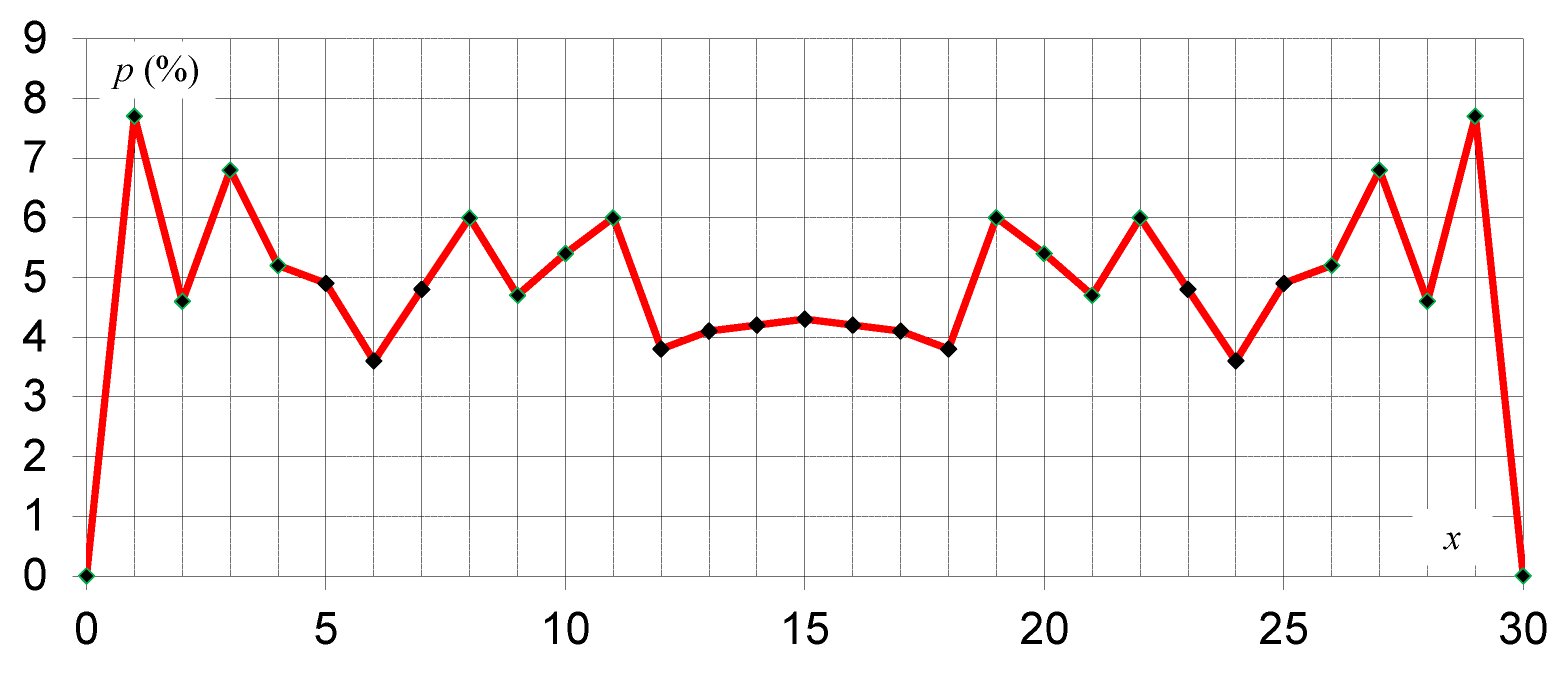
The values of the numbers constructing CIs with are given in Appendix A at entry and designated as , …, . The plot of Algorithm 1 CI non-coverage probabilities is given in Figure 1.
| Algorithm 1: BalancedCI |
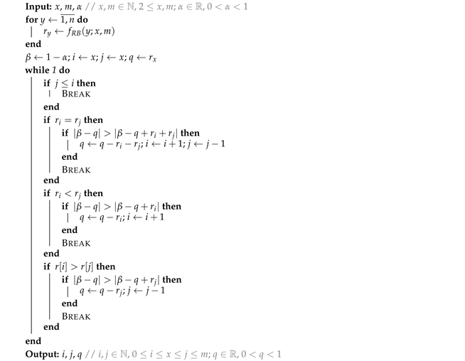 |

Figure 1.
Actual non-coverage probability (p) of BalancedCI for a sample of and (red line is only for visual purposes, doesn’t have physical meaning).
The actual non-coverage of CIs provided by Algorithm 1 is not monotone (it alternates, on average, around the imposed level) but symmetric and convergent to it. With data in Appendix A, Table 2 statistics can be calculated; the average values converge slowly, ).
Table 2.
Actual non-coverage probability tendencies ().
In terms of computational complexity, Algorithm 1 for given , m, and x requires a number of steps to arrive from x ( and in Algorithm 1) to and (see the series of for m = 30, 45, 100, and 900 in Appendix A). The solution is nearby. In fact, Equation (2) is an estimate of the asymptotic interval. Computational time is then proportional to . The shortest computational time is for and (near 0; only evaluation of the function time since and always), while the longest is for x near (where evaluations are needed). Thus, Algorithm 1 complexity is . The algorithm speed can be increased too if an approximate solution is provided before the While loop. Algorithm 1 from [11] or , with Equation (2) can be used for this task.
4. Discussion
One major point is to provide simple answers to simple questions. Here are some:
4.1. Question 1
How to express the confidence interval for a variable?
Let us take with . Using Appendix A, we get (this is in the series) and (this is in the series). The BalancedCI at 95% desired coverage () is [23, 29], and its actual coverage is 94.8%.
4.2. Question 2
How should one deal with proportions instead of variables?
The main issue is people’s tendency to simplify. For instance, is often written as ; for , we write or , but it is, in fact, not the same thing when it comes to sampling.
The preference for real numbers is obvious: people are much more comfortable with them and they quickly indicate the order of magnitude (0.0…or 0.1…is close to 0, 0.8…or 0.9…is close to 1, 0.4…or 0.5…is close to 0.5), which allows for instant interpretation. At the same time, however, it lets something slip through the cracks. One can express (with three decimal places, for example) any real sub-unit number, but its exact value cannot be obtained as a proportion of two integers, except under certain conditions and very few situations (one of these being that the sample size is 1000; for the sample size 997, however, there is no non-trivial situation).
Thus, using the same numbers, for positive outcomes from trials, in order to pass along all information, a convention is first needed to express the proportion as is without simplifying it (proportion is then ), and the confidence interval is expressed accordingly with fractions too.
The BalancedCI at 95% desired coverage () for is , and its actual coverage is 94.8%.
4.3. Question 3
How should a real-world data analysis be conducted?
Let us provide the answer by taking one case study from the literature. In [12], a study was conducted with 20 patients subject to dermal regeneration template placement over areas with exposed bone/tendon prior split-thickness skin grafting, all being confirmed clinically and microbiologically negative for previously treated infection. Utilizing non-invasive fluorescence imaging, bacterial load was identified using a defined threshold in eight out of twenty patients. Out of eight, four developed an infection. Three of the four infections were positive for Pseudomonas.
There are certain sampling with replacement variables in the study data. Five research questions can be formulated (the null hypothesis is that the effect being studied does not exist; the observation can be merely by chance):
- Q3.1: Was the detection of the bacterial load with non-invasive fluorescence imaging statistically significant in the group, or can it be asserted as being observed by chance?Answer: The observed proportion was 8 out of 20. The sequence of integers for and is 0 0 0 1 1 2 3 4 4 5 6 7 8 9 10 11 13 14 16 18 20. The CI for is [4, 12]. The answer is Yes (detection of the bacterial load with non-invasive fluorescence imaging was statistically significant in the group), with a true risk (of being in error in the coverage) of 3.6%.
- Q3.2: Was the development of a bacterial infection a real risk for the patients following the procedure, or can it be asserted as being observed by chance?Answer: The observed proportion was 4 out of 20. Using the same sequence of integers, the CI for is [1, 7], and the answer is Yes (developing a bacterial infection was a real risk for the patients following the procedure), with a true risk of 4.3%.
- Q3.3: Was Pseudomonas a real threat for the patients following the procedure, or can it be asserted as being observed by chance?Answer: The observed proportion was 3 out of 20. Using the same sequence of integers, the CI for is [1, 6], and the answer is Yes (Pseudomonas was a real threat for the patients following the procedure), with a true risk of 6.1%.
- Q3.4: Was the development of a bacterial infection a real risk for the patients possessing bacterial load detected by non-invasive fluorescence imaging, or can it be asserted as being observed by chance?Answer: The observed proportion was 4 out of 8. The sequence of integers for and is 0 0 0 1 2 3 4 6 8. The CI for is [2, 6], and the answer is Yes (developing a bacterial infection was a real risk for the patients possessing bacterial load detected by non-invasive fluorescence imaging), with a true risk (of being in error in the coverage) of 7.0%.
- Q3.5: Was infection with Pseudomonas a real risk for the patients possessing bacterial load detected by non-invasive fluorescence imaging, or can it be asserted as being observed by chance?Answer: The observed proportion was 4 out of 8. The sequence of integers for and is 0 0 0 1 2 3 4 6 8. The CI for is [1, 5]. The answer is Yes (infection with Pseudomonas was a real risk for the patients possessing bacterial load detected by non-invasive fluorescence imaging), with a true risk (of being in error in the coverage) of 5.9%.
With the sampled data, the answer was Yes in all cases since .
4.4. Question 4
How is the proposed method positioned relatively to other methods from the scientific literature?
Any formula-based approach will have the same deficiency against proposed method as the Wald confidence interval (Equation (2)) does. In this category, included are Agresti-Coull [13] and Wilson [14] CIs, and lesser-known approaches, such as arcsine and logit [15].
Any probabilistic-based approach, such as Clopper–Pearson [3] and Blyth–Still–Casella [16], imposes an actual risk always less than or equal to imposed risk. Because of that, the actual risk is severely penalized and on average tends to be biased relative to the imposed value (their ideal actual coverage is approximated by for , being about 4.1% instead of 5% for ).
A probabilistic balanced approach, such as Jeffrey’s [17], will provide a good solution on average, but not the one with minimal deviation from the imposed level, as Algorithm 1 does.
5. Conclusions
For sampling with replacement, an algorithm was proposed for calculating the confidence interval for the variable that defines the number of successes. The interval is constructed so that it is as close as possible to the required significance level. The algorithm is useful for small samples, for which the approximation to normality cannot be accepted, but the simplicity of its construction makes it applicable to practically any sample volume from real-world applications. The solution proposed by the algorithm is the construction of a sequence of monotonically increasing integers (between 0 and the volume of the sample), with which the confidence interval is constructed. Thus, if is the series of numbers (with x from 0 to m, several cases being listed in Appendix A), then the sequence of confidence intervals for the variable x extracted with replacement from the sample of volume m is .
Funding
No funding received for conducting this study.
Data Availability Statement
Raw data provided in the manuscript.
Acknowledgments
Help from editorial board and reviewers in improving this work is acknowledged.
Conflicts of Interest
The author declares no conflicts of interest.
Appendix A
Here, the ordered integer sequences, to be used for generating 95% coverage confidence intervals (CIs) for sampling with replacement variables, are given. For other coverage levels, Algorithm 1 should be used to generate new series.
- For a variable x from a sample of size m, the interval is .
- For a proportion , the interval is .
Each entry has numbers in the series (from to ). Ordered integer sequences are obtained with Algorithm 1 given in the paper.
The following notations have been used within the manuscript:
- : ceil function (smallest integer greater than);
- : floor function (greatest integer smaller than);
- : closed interval;
- : significance level;
- CI: confidence interval;
- p: non-coverage probability;
- , .
Appendix A.1. Ordered Integer Sequence for α = 0.05 and m = 30
0 0 0 1 1 2 2 3 4 5 6 7 7 8 9 10 11 12 13 14 15 16 18 19 20 21 23 24 26 28 30
Appendix A.2. Ordered Integer Sequence for α = 0.05 and m = 45
0 0 0 0 1 2 2 3 4 4 5 6 7 8 9 10 10 11 12 13 14 15 16 17 18 19 20 21 22 23 24 25 26 27 29 30 31 32 34 35 36 38 39 41 43 45
Appendix A.3. Ordered Integer Sequence for α = 0.05 and m = 100
0 0 0 0 1 2 2 3 3 4 5 6 6 7 8 9 10 10 11 12 13 14 15 15 16 17 18 19 20 21 22 23 24 25 25 26 27 28 29 30 31 32 33 34 35 36 37 38 39 40 41 41 42 43 44 45 47 48 49 50 51 52 53 54 55 56 57 58 59 60 61 62 63 65 66 67 68 69 70 71 72 74 75 76 77 78 79 81 82 83 84 86 87 88 90 91 92 94 96 98 100
Appendix A.4. Ordered Integer Sequence for α = 0.05 and m = 900
0 0 0 0 1 1 2 3 3 4 5 5 6 7 8 8 9 10 11 11 12 13 14 14 15 16 17 18 19 19 20 21 22 23 24 24 25 26 27 28 29 30 30 31 32 33 34 35 36 36 37 38 39 40 41 42 43 43 44 45 46 47 48 49 50 51 51 52 53 54 55 56 57 58 59 60 60 61 62 63 64 65 66 67 68 69 69 70 71 72 73 74 75 76 77 78 79 80 80 81 82 83 84 85 86 87 88 89 90 91 91 92 93 94 95 96 97 98 99 100 101 102 103 104 104 105 106 107 108 109 110 111 112 113 114 115 116 117 118 119 119 120 121 122 123 124 125 126 127 128 129 130 131 132 133 134 134 135 136 137 138 139 140 141 142 143 144 145 146 147 148 149 150 151 152 152 153 154 155 156 157 158 159 160 161 162 163 164 165 166 167 168 169 170 171 172 172 173 174 175 176 177 178 179 180 181 182 183 184 185 186 187 188 189 190 191 192 193 194 195 195 196 197 198 199 200 201 202 203 204 205 206 207 208 209 210 211 212 213 214 215 216 217 218 219 220 221 222 222 223 224 225 226 227 228 229 230 231 232 233 234 235 236 237 238 239 240 241 242 243 244 245 246 247 248 249 250 251 252 253 254 255 255 256 257 258 259 260 261 262 263 264 265 266 267 268 269 270 271 272 273 274 275 276 277 278 279 280 281 282 283 284 285 286 287 288 289 290 291 292 293 294 295 296 297 298 298 299 300 301 302 303 304 305 306 307 308 309 310 311 312 313 314 315 316 317 318 319 320 321 322 323 324 325 326 327 328 329 330 331 332 333 334 335 336 337 338 339 340 341 342 343 344 345 346 347 348 349 350 351 352 353 354 355 356 357 358 359 360 361 362 363 364 365 366 367 368 369 370 371 372 373 374 375 376 376 377 378 379 380 381 382 383 384 385 386 387 388 389 390 391 392 393 394 395 396 397 398 399 400 401 402 403 404 405 406 407 408 409 410 411 412 413 414 415 416 417 418 419 420 421 422 423 424 425 426 427 428 429 430 431 432 433 434 435 436 437 438 439 440 441 442 443 444 445 446 447 448 449 450 451 452 453 454 455 456 457 458 459 460 461 462 463 464 465 466 467 468 469 470 471 472 473 474 475 476 477 478 479 480 481 482 483 484 485 486 487 488 489 490 491 492 493 494 495 496 497 498 499 500 501 502 503 504 505 506 507 508 509 510 511 512 513 514 515 517 518 519 520 521 522 523 524 525 526 527 528 529 530 531 532 533 534 535 536 537 538 539 540 541 542 543 544 545 546 547 548 549 550 551 552 553 554 555 556 557 558 559 560 561 562 563 564 565 566 567 568 569 570 572 573 574 575 576 577 578 579 580 581 582 583 584 585 586 587 588 589 590 591 592 593 594 595 596 597 598 599 600 601 602 603 604 605 606 607 608 609 611 612 613 614 615 616 617 618 619 620 621 622 623 624 625 626 627 628 629 630 631 632 633 634 635 636 637 638 639 640 641 643 644 645 646 647 648 649 650 651 652 653 654 655 656 657 658 659 660 661 662 663 664 665 666 667 669 670 671 672 673 674 675 676 677 678 679 680 681 682 683 684 685 686 687 688 689 690 691 693 694 695 696 697 698 699 700 701 702 703 704 705 706 707 708 709 710 711 713 714 715 716 717 718 719 720 721 722 723 724 725 726 727 728 729 730 732 733 734 735 736 737 738 739 740 741 742 743 744 745 746 747 749 750 751 752 753 754 755 756 757 758 759 760 761 762 763 765 766 767 768 769 770 771 772 773 774 775 776 777 779 780 781 782 783 784 785 786 787 788 789 790 792 793 794 795 796 797 798 799 800 801 802 804 805 806 807 808 809 810 811 812 813 815 816 817 818 819 820 821 822 823 824 826 827 828 829 830 831 832 833 835 836 837 838 839 840 841 842 844 845 846 847 848 849 850 852 853 854 855 856 857 859 860 861 862 863 864 866 867 868 869 870 872 873 874 875 877 878 879 880 882 883 884 885 887 888 890 891 892 894 896 898 900
References
- Bernoulli, J. Ars Conjectandi; Inpenfis Thurnsiorum Fratum: Basel, Switzerland, 1713; Available online: http://sheynin.de/download/bernoulli.pdf (accessed on 10 March 2025).
- Andrews, G.E. The Geometric Series in Calculus. Am. Math. Mon. 1998, 105, 36–40. [Google Scholar] [CrossRef]
- Clopper, C.J.; Pearson, E.S. The use of confidence or fiducial limits illustrated in the case of the binomial. Biometrika 1934, 26, 404–413. [Google Scholar] [CrossRef]
- Blyth, C.R.; Still, H.A. Binomial confidence intervals. J. Am. Stat. Assoc. 1983, 78, 108–116. [Google Scholar] [CrossRef]
- Wald, A. Contributions to the theory of statistical estimation and testing hypotheses. Ann. Math. Stat. 1939, 10, 299–326. [Google Scholar] [CrossRef]
- Korn, E.L.; Graubard, B.I. Confidence intervals for proportions with small expected number of positive counts estimated from survey data. Surv. Methodol. 1998, 24, 193–201. [Google Scholar]
- Bolboacă, S.D.; Jäntschi, L. Optimized confidence intervals for binomial distributed samples. Int. J. Pure Appl. Math. 2008, 47, 1–8. [Google Scholar]
- Mishra, R.; Singh, R.; Raghav, Y.S. On combining ratio and product type estimators for estimation of finite population mean in adaptive cluster sampling design. Braz. J. Biom. 2024, 42, 412–420. [Google Scholar] [CrossRef]
- Ahmadini, A.A.H.; Singh, R.; Raghav, Y.S.; Kumari, A. Estimation of population mean using ranked set sampling in the presence of measurement errors. Kuwait J. Sci. 2024, 51, 100236. [Google Scholar] [CrossRef]
- Raghav, Y.S.; Ahmadini, A.A.H.; Mahnashi, A.M.; Rather, K.U.I. Enhancing estimation efficiency with proposed estimator: A comparative analysis of Poisson regression-based mean estimators. Kuwait J. Sci. 2025, 52, 100282. [Google Scholar] [CrossRef]
- Jäntschi, L. Binomial distributed data confidence interval calculation: Formulas, algorithms and examples. Symmetry 2022, 14, 1104. [Google Scholar] [CrossRef]
- Viana, E.H. 562 Bacterial Fluorescence Signals Are Associated with Dermal Regeneration Template Infections in Burn Patients. J. Burn Care Res. 2025, 46, S149. [Google Scholar] [CrossRef]
- Agresti, A.; Coull, B.A. Approximate is better than "exact" for interval estimation of binomial proportions. Am. Stat. 1998, 52, 119–126. [Google Scholar] [CrossRef] [PubMed]
- Wilson, E.B. Probable inference, the law of succession, and statistical inference. J. Am. Stat. Assoc. 1927, 22, 209–212. [Google Scholar] [CrossRef]
- Brown, L.D.; Cai, T.T.; DasGupta, A. Interval Estimation for a Binomial Proportion. Stat. Sci. 2001, 16, 101–133. [Google Scholar] [CrossRef]
- Casella, G. Refining binomial confidence intervals. Can. J. Stat. 1986, 14, 113–129. [Google Scholar] [CrossRef]
- Jeffreys, H. An invariant form for the prior probability in estimation problems. Proc. R. Soc. Lond. Ser. A Math. Phys. Sci. 1946, 186, 453–461. [Google Scholar] [CrossRef]
Disclaimer/Publisher’s Note: The statements, opinions and data contained in all publications are solely those of the individual author(s) and contributor(s) and not of MDPI and/or the editor(s). MDPI and/or the editor(s) disclaim responsibility for any injury to people or property resulting from any ideas, methods, instructions or products referred to in the content. |
© 2025 by the author. Licensee MDPI, Basel, Switzerland. This article is an open access article distributed under the terms and conditions of the Creative Commons Attribution (CC BY) license (https://creativecommons.org/licenses/by/4.0/).