Abstract
Temperature prediction plays a crucial role across various sectors, including agriculture and climate research. Understanding weather patterns, seasonal shifts, and climate dynamics heavily relies on accurate temperature forecasts. This paper presents an innovative hybrid method, EEMD-LR, that combines ensemble empirical mode decomposition (EEMD) with linear regression (LR) for temperature prediction. EEMD is used to decompose temperature signals into stable sub-signals, enhancing their predictability. LR is then applied to forecast each sub-signal, and the resulting predictions are integrated to obtain the final temperature forecast. The proposed EEMD-LR model achieved RMSE, MAE, and R2 values of 0.000027, 0.000021, and 1.000000, respectively, on the sine simulation time-series data used in this study. For actual temperature time-series data, the model achieved RMSE, MAE, and R2 values of 0.713150, 0.512700, and 0.994749, respectively. The experimental results on these two datasets indicate that the EEMD-LR model demonstrates superior predictive performance compared to alternative methods.
1. Introduction
Temperature prediction plays a crucial role in modern society, with applications spanning across multiple fields [1]. Firstly, temperature prediction can assist meteorological departments in issuing early warnings for weather-related disasters, thereby reducing casualties and property losses. Secondly, the temperature is a vital factor in the growth and development of crops, so accurate temperature prediction helps to increase crop yields and ensure food security. Additionally, temperature prediction is of significant importance in transportation, energy production and supply [2], urban planning [3], health management [4], and disease control, as well as environmental protection [5] and ecological balance. Therefore, continuously improving the accuracy and reliability of temperature prediction is essential for addressing climate change [6], ensuring public safety, and promoting sustainable development.
Temperature prediction serves domain-specific critical functions: agriculture relies on growing-degree days (GDD) forecasts to optimize crop cycles; energy systems use hourly load predictions to prevent grid failures; public health organizations employ heatwave alerts to reduce mortality; transportation requires road-surface temperature forecasts for accident prevention; and climate policy depends on decadal projections for emission strategies. Each application demands distinct prediction horizons and accuracy thresholds, collectively justifying the need for modeling that is robust against inherent non-stationarity and noise.
Temperature prediction has a significant impact on agricultural production [7] and food security. Temperature is one of the key factors that affects crop growth and development, and its accurate prediction helps farmers in making informed decisions regarding the planting time, fertilization, and irrigation of their crops, as well as other agricultural activities. This, in turn, leads to increased crop yield and quality, ensuring food supply and agricultural product safety [8].
Temperature prediction also holds significant importance in energy production and supply, transportation, urban planning, health management, and disease control, as well as environmental protection and ecological balance. In terms of energy production and supply, accurate temperature prediction assists the power and gas industries in effectively planning their energy supply, improving energy utilization efficiency and reducing energy costs. Concerning transportation and urban planning, temperature prediction helps transportation management departments in implementing effective traffic control measures, reducing traffic congestion and accidents, and enhancing the efficiency of urban transportation. Regarding health management and disease control, the temperature directly impacts human health, so accurate temperature prediction aids health departments and medical institutions in taking timely measures to prevent and address temperature-related health issues. In certain specific fields, such as greenhouse temperature control (e.g., MPC and RL optimizations [9], GRU-based multi-scale predictions [10]), photovoltaic panel temperature modeling (hybrid numerical-ML methods [11]), and soil temperature estimation (spatiotemporal deep learning frameworks [12]), effective temperature management and prediction are required. In the realm of environmental protection and ecological balance, temperature prediction contributes to monitoring and assessing the quality of the environmental, preventing and reducing environmental pollution, protecting ecosystems and biodiversity, and promoting sustainable development and ecological balance.
The current methods for temperature prediction include traditional physical model approaches and data-driven machine learning methods. Here are some common temperature prediction methods.
First, the traditional numerical [13] weather prediction models entail a forecasting method based on atmospheric physics equations and numerical calculation techniques. These models divide the atmosphere into three-dimensional grids and simulate atmospheric dynamics and thermodynamics processes to predict temperature changes over a future period of time. Some of the well-known prediction models for weather include the Medium-Range Weather Forecasts of European Centre, the Global Forecast System (GFS), and Environmental Prediction, which was developed by the National Centers, among others. These models provide high-resolution weather forecasts and are suitable for short-term and medium-term predictions.
Second, statistical methods [14] represent an approach that uses historical observation data and statistical models to forecast future temperature changes. These methods include time-series analysis, regression analysis, and probabilistic statistical methods, among others. Statistical methods are commonly used for short-term and medium-term weather forecasts, particularly when complex physical process simulations are not available. They can provide simple and effective predictions.
Third, machine learning methods [15,16] have gained attention in recent years as a temperature prediction approach. These methods utilize a large amount of observation data and model input data to train machine learning models to forecast future temperature changes. Typical machine learning techniques encompass support vector machines, decision trees, deep learning methods, neural networks, and various other approaches. These methods are suitable for long-term and global-scale climate simulations and can handle complex nonlinear relationships and multivariate data, achieving certain prediction results.
Fourth, the ensemble forecast method [17] is an approach that enhances the accuracy of temperature prediction by constructing a collection of models with different initial conditions or parameter settings, and then conducting statistical analysis on these model ensembles. This method effectively reduces the predictive errors of individual models and thereby improves the reliability and confidence of forecasts. It is commonly used for long-term and global-scale predictions [18]. In fact, methods can be diverse and mixed methods, such as Bayesian models for probabilistic temperature prediction, physical information neural networks for heat transfer modeling, and “perfect model” framework research for regional climate prediction [19].
Fifth, time-series analysis [20,21,22,23] is a statistical method used to forecast temperature changes. It identifies temperature change patterns by examining the periodicity, trend, and seasonality in historical data. Secondly, it utilizes models such as ARMA, ARIMA, etc., to fit the historical data and predict future temperatures. It has an improved prediction accuracy due to incorporating external factors such as meteorological data. Although it cannot capture complex processes, it has certain applications in short-term and medium-term forecasts. Some studies have used mixed time-series methods, and here are some references to groundbreaking work—the CEEMDAN-PSO hybrid model [24] for price prediction—and recent developments—the HHO-LSTM-SVR [25] for TBM parameter prediction and the ARIMA-ANN hybrid model [26] for high-frequency financial data.
Sixth, data assimilation techniques [27,28] involve combining observational data with numerical model simulations and using optimization methods to adjust the model state, which enhances the temperature prediction accuracy of the model. Data assimilation techniques can effectively utilize multiple sources of observational data, correct model errors and uncertainties, and improve the spatial and temporal resolution of temperature predictions. It is an important means of improving the accuracy of temperature prediction.
Finally, transformer-based models [29] have demonstrated significant advantages in time-series forecasting. They effectively capture complex relationships and pattern changes within time series through self-attention mechanisms, which makes them suitable for applications such as stock market prediction and climate change modeling. Various improved models, such as GPHT, ShapeFormer, TFT, and FLUID-GPT [30], have been proposed to enhance the forecasting performance and applicability of existing models. These models can handle long sequence data, capture long-range dependencies, and provide interpretable insights. However, transformer models can be computationally intensive when dealing with time series and require substantial amounts of data, so considerations of computational resources and data availability are necessary in practical applications. Reference [29] proposes using Transformer models for predicting dynamic systems that represent physical phenomena. By employing Koopman-based embeddings, dynamic systems are projected into vector representations, which are then predicted by the Transformer model. The proposed approach outperforms traditional methods that are commonly used in scientific machine learning, which demonstrates its effectiveness. Reference [30] introduces the FLUID-GPT model for predicting particle trajectories and erosion in industrial-scale steam pipelines. FLUID-GPT combines GPT-2 and CNN, requiring only five initial conditions for accurate erosion prediction. Compared to BiLSTM, FLUID-GPT exhibits significant improvements in both its accuracy and efficiency.
Although current temperature prediction methods have achieved certain success in various scenarios and time scales, there are still some challenges. The complexity and uncertainty of temperature prediction make forecasting difficult, and the mismatch between different scales limits the applicability of the existing models. This paper combines multiple methods for temperature prediction and has achieved good results in experiments.
The remainder of this document is structured as outlined below: A brief overview of relevant concepts, terminologies, and the EEMD and LR techniques is provided in Section 2. Following that, Section 3 showcases the combined approaches for short-term temperature prediction using ensemble EMD with LR. Moving on to Section 4, we focus on the introduction of the experimental data utilized in this research. Section 5 details the experimentation through simulation and the subsequent empirical analysis of the proposed methodologies. The concluding section summarizes key findings and highlights potential future endeavors.
2. Ensemble EMD with LR Related Works
To enhance the accuracy of temperature forecasting, a novel approach for temperature prediction that combines ensemble empirical mode decomposition (EEMD) with linear regression (LR) has been introduced as LR-EEMD. Drawing inspiration from the divide-and-conquer strategy for tackling complex issues and the iterative optimization approach of machine learning, this hybrid method aims to improve on the temperature prediction performance of existing models. This paper begins by introducing the fundamental concepts and terminologies, which is followed by a detailed discussion on the application of EEMD and LR. Additionally, empirical mode decomposition (EMD) will be introduced in relation to this study.
2.1. EMD
EMD is the abbreviation for empirical mode decomposition. It is a signal processing approach introduced by Huang et al. in 1998 [31]. It addresses the challenges posed by traditional decomposition methods when dealing with non-stationary and nonlinear signals. Instead of relying on predefined assumptions, EMD adaptively breaks down signals into components known as IMFs (intrinsic mode functions), with each capturing specific frequency and amplitude characteristics. This technique stands out for its ability to capture local signal nuances.
The EMD algorithm follows a straightforward “sifting and extraction” process. Initially, it constructs lower and upper boundaries using local extrema points, then iteratively computes IMFs by subtracting the mean of these envelopes. The process continues until certain IMF criteria are met, which results in a set of IMFs and a residue term. These IMFs represent the signal’s oscillatory behavior across different time scales.
EMD’s strength lies in its data-driven approach, which eliminates the need for predefined assumptions about the signal. This versatility makes it suitable for diverse signal types, including nonlinear and non-stationary ones. Moreover, EMD excels in capturing local signal details, which leads to higher fidelity decomposition outcomes.
In practical applications, EMD finds utility in various signal processing tasks. It can effectively denoise signals by selectively filtering high-frequency IMFs while preserving critical signal features. Additionally, EMD facilitates signal analysis by revealing the main characteristics of the signal through the examination of IMFs at different frequencies. Its versatility and effectiveness make it a valuable tool in signal processing contexts.
When dealing with specific types of signals, the traditional EMD method may face challenges such as mode mixing and over-decomposition. In such cases, multiple intrinsic mode functions (IMFs) with similar characteristic frequencies can lead to confusion, which can make it challenging to interpret and analyze the signal characteristics. This situation is referred to as mode mixing. Additionally, traditional EMD’s tendency to extract numerous IMFs from a signal can lead to over-decomposition and result in an excessive number of IMFs, some of which may contain noise or irrelevant components and thereby complicate the process of signal analysis.
In 2009, Wu and colleagues introduced an adaptive empirical mode decomposition technique (EEMD) [32]. It leverages the statistical properties of white noise signals. EEMD tackles these challenges by incorporating random noise. More specifically, it integrates different random noises with the initial signal. It reconstructs the signal repeatedly, using a distinct random noise profile each time. This iterative process results in the generation of subtly varying intrinsic mode functions (IMFs) with each reconstruction, which enhances the model’s diversity in capturing the signal’s structural characteristics. Subsequently, the outcomes of multiple reconstructions are averaged to yield the final IMF. This holistic approach aids in mitigating mode mixing by exploiting the slight deviations in the IMFs produced during each reconstruction, and allows for more comprehensive capturing of the signal’s attributes. Furthermore, averaging the outcomes of multiple reconstructions can mitigate over-decomposition by potentially nullifying irrelevant IMFs in the averaging process.
Based on recent studies, EEMD has demonstrated significant advancements in processing non-stationary signals across diverse domains:
- (1)
- Biomedical signal denoising: EEMD combined with modified sigmoid thresholding effectively reduces noise in ECG signals while preserving QRS complexes and enhancing feature extraction for clinical diagnosis [33]. Novel approaches like EEMD-MD (Mahalanobis distance) further improve the noise separation in finger-based ECG by quantifying the probability density functions of IMFs [34];
- (2)
- Industrial vibration analysis: Enhanced EEMD algorithms with multi-sensor fusion and minimum lower-bound frequency selection enable the precise denoising of acoustic signals from high-voltage shunt reactors. This method eliminates environmental noise interference and accurately assesses the health of equipment [35];
- (3)
- Financial forecasting [36]: Integrated into hybrid frameworks (e.g., EEMD-SE-GA-GRU), EEMD decomposes nonlinear stock market data (e.g., Dow Jones Index) into multi-scale IMFs. Clustering IMFs by their sample entropy (SE) complexity reduces the input dimensions by 38%, significantly boosting the prediction accuracy of this approach (R2 = 0.9814);
- (4)
- Geophysical signal processing [37]: While newer variants like SVMD dominate marine MT data denoising, EEMD-inspired decomposition principles underpin noise suppression in wave-induced electromagnetic interference, which improves the subsurface electrical structure analysis of this approach;
- (5)
- Environmental modeling: Some studies apply EEMD to PM2.5 prediction (e.g., EEMD-SSA-LSTM, EEMD-ALSTM [38]), and the development of an EEMD-CNN-BiLSTM water environmental indicators prediction method [39] highlights the successful application of EEMD in the field of meteorology. In terms of model comparison, this method mainly includes integrated benchmarks in LSTM, SVR, and urban air quality index prediction research (for example, LSTM-SVR hybrid models are superior to individual models [40]), as well as GIS transformer frameworks for irregular time series [41], and so on.
These applications highlight EEMD’s adaptability in isolating signal components from noise-polluted, non-linear data through adaptive IMF extraction and ensemble averaging.
In summary, EEMD enhances the robustness and dependability of signal decomposition through the incorporation of stochastic elements and integration methodologies. This enables it to effectively address challenges like mode mixing and over-decomposition that are prevalent in traditional EMD methods, which renders it a more potent and trustworthy tool for managing diverse signal types.
In the process of using EEMD, the initial task involves identifying the characteristics of the random noise and establishing the number of iterations. Afterward, this noise is merged with the initial signal to create numerous unique random experiments. Each experiment involves combining the initial signal with varying random noise to generate multiple versions featuring diverse random disturbances. Subsequently, EMD is utilized on each noisy signal experiment to derive a collection of IMFs. Ultimately, the outcomes from each experiment pertaining to the identical IMF component are averaged to yield resilient IMFs. Below is a concise overview of the procedure for decomposing time series using EEMD.
- (1)
- Initialization
Assume that there is an initial signal x(t), along with EEMD parameters (such as iteration count, noise standard deviation, etc.), and that the selection of the type and parameters of the random noise is to be conducted.
- (2)
- Generate random experiments
For each experiment (i = 1, 2, …, n), generate random noise sequences Ni(t) of the same length. The random noise can be Gaussian noise or a uniformly distributed random sequence.
- (3)
- Add random noise
Combine each random noise sequence with the initial signal to obtain signal experiments with noise yi(t) = x(t) + Ni(t).
- (4)
- Run EMD
Apply the EMD algorithm to each signal experiment with noise yi(t), decomposing it into a set of IMFi (i = 1, 2, …, ) as demonstrated in Equation (1).
where is the i-th IMF in the experiment, and is the residual term.
The initial signal depicted by the black line in Figure 1 is processed using a cubic spline interpolation approach that identifies the local minimum and maximum values. This process generates lower and upper envelope lines, which are represented by the red and blue lines in Figure 1, respectively.
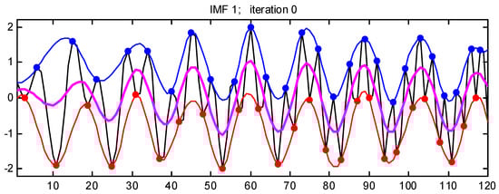
Figure 1.
The process of EEMD decomposition.
- (5)
- Compute average IMF
For each IMFi (i = 1, 2, …, ) component, calculate the average value of the same IMF component across all experiments.
- (6)
- Reconstruct the signal
Reconstruct the signal as the sum of all average IMFs and the residual term as shown in Equation (2).
The quantity of sub-time series, denoted by k in Equation (2), is contingent upon the complexity of the initial time series.
- (7)
- Termination
Output the reconstructed signal , along with the obtained IMFs. Figure 2 illustrates the EEMD decomposition process for the sin time series described in Equation (3).
where .
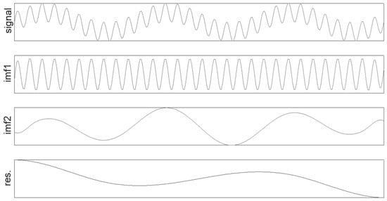
Figure 2.
Sin EEMD decomposition chart.
2.2. Linear Regression
The linear regression (LR) model [42], a statistical tool, is utilized to establish linear connections between variables. By capturing the linear correlation between the independent variables (features) and the dependent variable, this model enables the prediction of unknown observations. When applied to temperature prediction, the LR model can be used to scrutinize the correlation between the temperature and various influencing factors such as the season, geographic location, altitude, and more. By gathering historical temperature data and data associated with these factors as independent variables, the LR model can formulate the mathematical relationship between the temperature and these factors. Subsequently, leveraging this relationship, the LR model can make forecasts about future temperatures. This methodology can benefit meteorologists, agricultural specialists, urban planners, and others by leveraging past data to forecast upcoming temperature changes, and thereby facilitates informed decision-making and planning [43]. Below is a concise overview of the procedure involved in decomposing data using the LR technique.
The simplest and most straightforward relationship between feature x and target y is a linear relationship. Each feature is associated with a weight that directly influences the expression of the target.
Assume that the linear model is constructed with the expression shown in Equation (4).
where represents the input t-dimensional feature vector, also known as the independent variables. Y is the target and also the dependent variable. is termed the intercept; (, , …, , ) are referred to as the slope coefficients; is the error term, which is independent of the model and follows a normal distribution N(0, ).
In a figurative sense, the linear model adheres to the LINE criteria. Here, L represents linearity, which indicates that the correlation between the target and the independent variables is linear. I stands for independence, denoting that the error terms are mutually independent. N signifies normality, which suggests that the error terms follow a normal distribution. E denotes equal variance, which indicates that error terms have constant variance.
Actually, Equation (4) can be simplified into Equation (5).
Here, , , , and , in Equation (5), respectively, can be substituted for Equations (6)–(9).
where the in the above equations represent the transposition of the matrix.
The model’s goodness is generally evaluated by the sum of the squared residuals, as shown in Equation (10). Equation (10) is commonly referred to as the residual sum of squares (RSS).
During experiments, the aim is to minimize this loss by adjusting ; thus, becomes the coefficients to be estimated for the model. Linear regression is a convex optimization problem, with its loss function being strictly convex. There must exist an optimal value within the interval; thus, Equation (11) exists.
This equation requires that is invertible, which involves linear space theory and requires solving cases accordingly.
If is invertible, it means that only the vector exists such that , and that and have the same null space. Therefore, it necessitates that is full rank, meaning that the columns of are linearly independent among the samples.
When is not invertible, it implies that does not satisfy full rank, indicating linear correlation among multiple input samples. This means that at least one sample can be represented through a linear blend of other samples, which is termed as having perfect multicollinearity among the independent variables. In such cases, it is necessary to remove variables that are linear combinations of others, or collect more features to ensure that no linear relationships exist among the samples.
When is invertible but some samples are nearly expressible as linear combinations of others, it indicates the presence of near multicollinearity among the variables. In this scenario, dimensionality reduction techniques can be employed to address this issue.
Here is the reasoning process for whether there exists an optimal solution for simple linear regression, which is a simplification of Equation (11) to Equation (12).
Following this are Equations (13) and (14).
where is the sample mean, is the target mean, and and are the parameters that we estimate.
It is worth noting that the aforementioned simple linear regression does have an optimal solution. It requires calculating the Hessian matrix of the loss, as shown in Equation (15).
It is easy to observe that seeking the eigenvalues of H is equivalent to determining the eigenvalues of the matrix A, as shown in Equation (16). The eigenvalues of matrix A are represented as shown in Equation (17).
Equation (17) transforms into Equation (18) after the matrix operations.
Through simple mathematical reasoning, it is easy to see that Equation (19) is non-negative, that is, greater than or equal to zero.
Therefore, Equation (17) has two roots. One root is greater than 0, while the other root is greater than or equal to 0. The eigenvalue of Equation (18) is 0 only when the condition that Equation (19) is 0 holds. Hence, it is inferred that matrix A is positive definite or semi-definite, which implyes that matrix H is also positive definite or semi-definite. Consequently, the loss function is convex, and it can be solved using convex optimization (such as quasi-convex optimization) or gradient descent methods.
2.3. Gradient Descent
The purpose of gradient descent is to find the minimum value of the cost function. The cost functions primarily include the mean squared error (MSE), the calculation formula for which is shown in Equation (10), and the cross-entropy loss (CEL) function, which is shown in Equation (20). The mean squared error is commonly employed to measure the error between predicted values and true values in prediction tasks. The CEL is frequently employed to measure the error between predicted probabilities and true labels in classification tasks.
where represents the predicted probability, represents the true label, m denotes the quantity of categories, and n denotes the quantity of samples.
Suppose that there is a function z = f(x,y) that is defined in a neighborhood U(P) of point P(x,y). From point P, let us draw a ray l. If the limit shown in Equation (21) exists, it is called the directional derivative of point (x,y) along the direction of l, and is denoted by .
Clearly, numerous rays, l, can be found, which indicates that there are infinite directional derivatives. However, the focus is typically on the maximum one, which signifies the direction in which the function changes the fastest; this is what is commonly referred to as the gradient.
The derivative of the loss function is the focal point of attention. The direction of the smallest negative gradient of the loss is the quickest path to reduction. If this direction is optimized, the loss decreases even faster.
Sometimes, it is not necessary for the line fitted through a large set of data to pass through the origin. In such cases, an additional parameter needs to be introduced. Consequently, the graph of forms a surface.
Gradient descent can be imagined as descending a mountain, as shown in Figure 3. How do you descend from a high mountain to its base as quickly as possible? The answer is to start from any position, find the steepest direction at that point, walk a distance along that direction, and then, at each step, reassess the steepest direction at the current position. Continue this process, walking along the newly identified direction, to descend to the base of the mountain as quickly as possible. During this descent, it is crucial to confirm the steepest direction at each step. The key lies in determining the “steepest direction,” with the direction of the largest gradient indicating the steepest descent direction.
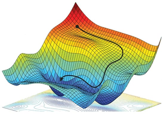
Figure 3.
Gradient descent process diagram.
During the descent down the mountain, at each step, a new direction needs to be determined. Constantly determining new directions implies that the parameters of the cost function are continuously changing. To obtain new parameters, it is necessary to update them based on the known old parameters. This requires repeatedly updating the parameters, a process known as batch gradient descent, as shown in Equations (22)–(24).
where is the learning rate, determining how large the steps are that are taken during the descent. The purpose of the derivative is to determine the direction of the descent. The on the right side is the old parameter, while the on the left side is the new parameter. At each step (each iteration), a new parameter needs to be determined, and only by updating the parameters can the direction for the next step be determined.
In summary, first, initialize the current position, calculate the position after one step of gradient descent according to the formula, and then, based on this position, subtract the product of the learning rate and the derivative at that point from the parameter value to obtain the position after one more step of gradient descent, i.e., the new parameter value. Repeat the above steps until the lowest point is reached. During this process, it is observed that, as the gradient descent progresses, the magnitude of movement of the point becomes smaller and smaller because, as the point descends, the value of the derivative decreases, while remains constant, which causes the step size to decrease.
2.4. LSTM Neural Network
Recurrent neural networks (RNNs) are primarily engineered to tackle nonlinear, time-varying issues. Their internal connections facilitate both forward and backward data propagation. Incorporating feedback loops enables convenient residual or weight updates during the forward pass. This capability proves particularly advantageous for time-series forecasting, empowering the extraction of patterns from historical data to predict future values. The fundamental architecture of an RNN is illustrated in Figure 4, where the leftmost column depicts the overarching RNN structure, while the rightmost column provides a detailed expansion thereof.
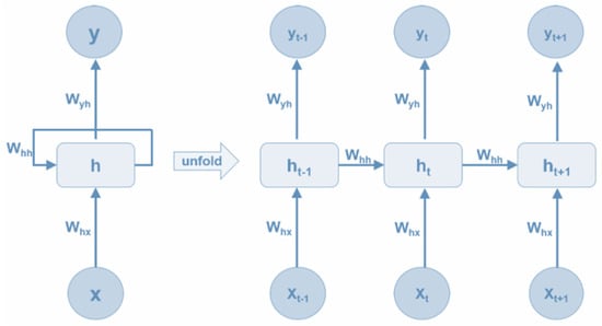
Figure 4.
Fundamental architecture of RNN.
The RNN module, denoted as in Figure 4, processes input data and yields an output at time . Unlike traditional neural networks, RNNs share the parameters , , and across each layer. This parameter sharing implies that every step within the RNN performs analogous operations, albeit on different input–output pairs . Consequently, the parameter space to be learned in RNNs is significantly reduced. As RNNs expand, they manifest as multilayer neural networks. In contrast to traditional setups where each layer possesses distinct parameters, RNNs maintain uniformity across layers. For instance, the parameters between the and layers remain consistent, as do those between the and layers. Likewise, the parameters between and and between between and remain identical throughout.
In the RNN, each step involves an output and input, but not every step’s input and output are crucial. Take predicting mathematical expression values as an example: we only need the output after inputting the last expression symbol, rather than that for each symbol input. The hidden layer of the RNN is its essence, being adept at capturing both short- and long-term information within time-series data. However, RNNs are plagued by the issue of vanishing gradients during network training. This issue can lead to indefinite increases in the training time, and can ultimately cause network paralysis. Hence, a simple RNN is suboptimal for predicting time series with long-term dependencies.
The LSTM neural network addresses the gradient vanishing issue encountered by simple RNNs when dealing with time series with long-term dependencies. It introduces output, input, and forget gates to the network model, which enhances its capabilities. These gates, illustrated in Figure 5, incorporate sigmoid activations, effectively combating gradient disappearance. The memory cell, a key innovation in LSTM, stores essential state information, enabling it to adeptly capture long-term dependencies. Each gate module typically employs an activation function to facilitate nonlinear transformations or information filtering. For instance, the forget gate ft decides which neuron state information to discard, enhancing the network’s adaptability.
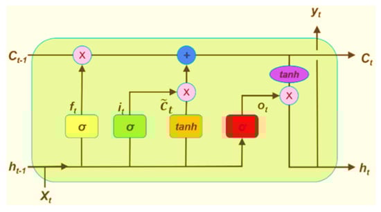
Figure 5.
Basic structure of LSTM.
2.5. Activation Function
Activation functions are pivotal in neural networks, serving to apply nonlinearity to weighted and summed input data. They introduce nonlinear elements that are critical for tackling problems beyond linear model capabilities. Without activation functions, neural network outputs would merely be linear combinations of preceding layer inputs, regardless of the network depth. These functions enable neural networks to approximate any arbitrary nonlinear function, expanding their problem-solving capacities beyond those of linear models.
Figure 6 and Figure 7 illustrate the curves of eight frequently employed standard activation functions, including the Softsign, ReLU, Tanh, Sigmoid, and Softplus functions. Here, we introduce the formulas of several typical activation functions. Equations (25)–(28) depict the formulas for the Sigmoid, Tanh, ReLU, and Softplus functions, respectively. Additionally, the softmax function, with slightly different formulas, finds primary application in multi-classification neural networks.
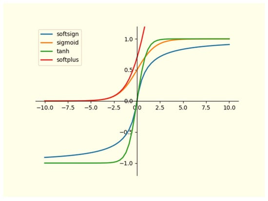
Figure 6.
The curves of four typical activation functions.
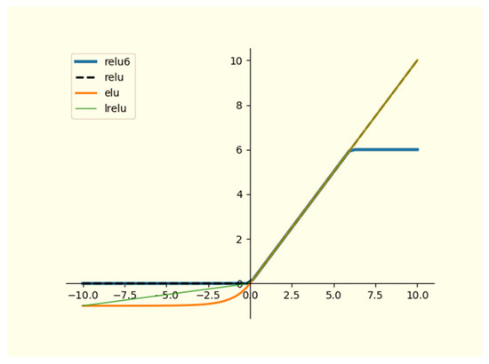
Figure 7.
The curves of four ReLU activation functions.
The ReLU function has been selected as the activation function for all gates in the LSTM in this study. For instance, Equation (29) depicts the function for the forgetting gate, which is denoted as ft.
Figure 5 illustrates the workflow of the LSTM. In each formula, Wi, Wf, Wc, and Wo denote the weight vectors, while bi, bo, bc, and bf denote the bias vectors. These elements are involved in various computations within the network:
- (1)
- The LSTM neural network receives external input data . It is combined with the output data to create the input data . Initially, this input data pass through the forgetting gate ft. Following activation function calculations shown in Equation (29), the resulting data from the forget gate, represented by ft, are acquired. This gate, ft, serves to dictate which neuron state information will be cleared.
- (2)
- Simultaneously, the input data are directed towards the input gate. Following the activation function calculations outlined in Equation (8), the output of the input is derived. This gate, denoted as , dictates the information to be updated and store within the memory neuron. Its function is described in Equation (30);
- (3)
- The input data are directed towards the tanh gate. Following the activation function calculations as outlined in Equation (31), the output of tanh is derived. This serves as the candidate vector produced by the tanh, and is utilized for updating the neuron state. Equation (31) describes the tanh gate function.
- (4)
- The updated state information is derived from the previous state information of the neuron, and is calculated using the function defined in Equation (32). This process involves the candidate vector , which determines the extent of state information to be updated.
- (5)
- Concurrently, the input data are directed towards the output gate. Following the activation function calculations shown in Equation (33), the output from the output gate is acquired. This gate, represented as , is governed by the function depicted in Equation (33).
- (6)
- Equation (34) illustrates the process for computing the output data . Initially, the activation function filters the neuron’s state information, which is then fed into the tanh gate. Multiplying the resulting output data of the output gate yields the output data .
3. Methodology
In this section, we present the foundational theory behind our proposed EEMD-LSTM and EEMD-LR prediction methods. Initially, we provide a brief overview of the EEMD, LSTM, and LR techniques discussed earlier. Subsequently, we delve into the basic structure of prediction methods for EEMD-LSTM and EEMD-LR, establishing the theoretical framework for our prediction methodologies [44]. Our approach involves decomposing complex wind speed sequences into low complexity sub-sequences using EEMD. These sub-sequences are then individually predicted by employing LR, LSTM, EEMD-LSTM, and EEMD-LR methodologies. The ultimate forecast for the initial sequence is obtained by aggregating the prediction values from multiple sub-sequences.
The models for EEMD-LSTM and EEMD-LR are depicted in Figure 8 and Figure 9, respectively. Additionally, Figure 10 illustrates the the proposed EEMD-LR. This approach aims to simplify complex problems by breaking them down into simpler ones, solving each to address the overall complexity. The fundamental operational process of EEMD-LR involves decomposing the problem into manageable subproblems and solving them individually to attain the overarching solution.

Figure 8.
Schematic diagram of EEMD-LSTM.
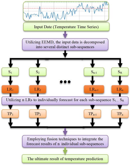
Figure 9.
Schematic diagram of EEMD-LR.
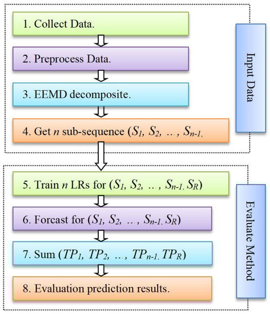
Figure 10.
Diagram outlining the proposed EEMD-LR.
Below are schematic diagrams of the models for the EEMD-LSTM and EEMD-LR methods. The models encompass five distinct steps: collect and prepare data, employ EEMD to decompose and to create various sub-sequences, train machine learning models separately for forecasting, aggregate prediction results from all sub-sequences, and evaluate the model. Figure 10 is a concise overview of the fundamental operational process of the EEMD-LR method. In short, Figure 10 illustrates the end-to-end workflow of the proposed EEMD-LR method: raw Signal → EEMD → IMFs → parallel LR models → ensemble prediction.
The novelty of combining EEMD with LR lies in leveraging EEMD’s ability to decompose complex time series into intrinsic mode functions, which can capture underlying patterns and trends more effectively. This decomposition enhances LR’s predictive accuracy by providing cleaner, more relevant features for regression analysis. By integrating these methods, our approach addresses limitations of traditional regression models, achieving an improved prediction performance on non-stationary or noisy data. This novel combination offers a more robust and accurate framework for time-series forecasting, which sets it apart from conventional methods that rely solely on linear regression or simpler decomposition techniques.
To clarify the EEMD–ML interaction, further explanation is provided on the relationships between important modules. After decomposing the raw temperature signal into IMFs via EEMD, each IMF (and residual) is treated as an independent input channel for the ML model. For linear regression (LR), each IMF component is fitted with a separate LR sub-model. Predictions from all sub-models are aggregated (summed) to produce the final output. Decomposition reduces nonlinearity in sub-signals, simplifying the modeling complexity. LR is applied to each IMF to capture linear trends at different frequency scales, which avoids the need for complex nonlinear architectures.
Below is a detailed description of the proposed method:
- (1)
- Simulation data are generated alongside the collection of real-world data, both of which undergo preprocessing to align with formatting requirements for the EEMD. This ensures the formation of the input data X for the EEMD;
- (2)
- The EEMD divides the input data X into n sub-sequences, adhering to the regulations of the decomposition for time series. Typically, the final sub-sequence is termed the residual sub-sequence SR. Hence, the n sub-sequences comprise n − 1 IMF sub-sequences and one residual sub-sequence SR, which is denoted as (S1, S2, …, Sn−1, SR). The data of each sub-sequence are partitioned into training and test sets. The training data are utilized for machine learning model training, while the testing data evaluate the trained model’s performance;
- (3)
- Each sub-sequence’s training data are implemented to sequentially train the corresponding model. For instance, the LSTM model is trained in the EEMD-LSTM and the LR in the EEMD-LR. These training processes are independent of each other. Following model training, we form the models LSTMi, and LRi (i = 1, 2, 3, …, n − 1, n). We then employ these trained models to forecast the respective test data of the sub-sequences, generating prediction results TPi (i = 1, 2, 3, …, n − 1, n);
- (4)
- Various fusion techniques are available for combining the prediction outcomes from numerous sub-sequences to derive the ultimate temperature prediction result. In this study, the chosen fusion technique is summation. This method entails aggregating the prediction outcomes of each individual sub-sequence test dataset and culminates in the final result of temperature prediction;
- (5)
- In conclusion, the forecasted outcomes are contrasted with the actual results from the test data utilizing three assessment standards (RMSE, MAE, and R2) to compute forecasting errors and assess the model’s strengths and weaknesses.
EEMD (ensemble empirical mode decomposition) is a data-driven decomposition method that is particularly effective in analyzing non-linear and non-stationary time-series data. Here are the reasons for using EEMD in our study:
- (1)
- Capturing intrinsic data characteristics: EEMD decomposes a time series into a set of intrinsic mode functions (IMFs) and a residual trend. This allows for a more flexible and detailed analysis of the data compared to traditional decomposition methods, which might not capture the inherent characteristics of non-stationary signals as effectively;
- (2)
- Noise reduction: EEMD enhances the ability to distinguish between noise and meaningful signals. By adding white noise to the data and averaging the results across multiple realizations, EEMD reduces the impact of noise and provides a clearer separation of signal components;
- (3)
- Improving analysis accuracy: The ability of EEMD to adapt to the data’s intrinsic properties helps in better capturing subtle patterns and features that might be missed by other methods. This is especially useful in complex datasets where traditional methods may not perform optimally.
In short, EEMD enhances the clarity of data by effectively separating noise from the signal, demonstrating robustness and revealing detailed insights through its decomposition of the data into IMFs and a residual trend.
The pseudocode for the EEMD-LR algorithm of our proposed model is shown in Algorithms 1–3.
| Algorithm 1: EEMD |
| Input: Time-series data x(t), number of ensembles N; |
| Output: Set of IMFs and residual trend (SR); |
| 1: Initialize: -Set number of ensembles N, -Set noise amplitude A; |
| 2: For each ensemble i from 1 to N do: |
| 3: Add white noise to the original signal: x_i(t) = x(t) + A * noise(t) |
| 4: Decompose x_i(t) into a set of IMFs and a residual trend: IMF_i, res_i = EMD(x_i(t)) |
| 5: Store the IMFs and residuals from this ensemble: SN_i = IMF_i; SR_i = res_i |
| 6: Average the IMFs and residuals over all ensembles: SN = Average(SN_i); SR = Average(SR_i) |
| 7: Return: (S1, S2, …, SN−1, SR). |
| Algorithm 2: LR |
| Input: Training dataset features F, labels L, number of iterations I; |
| Output: Optimized coefficients _opt |
| 1: Initialize: Initialize coefficients: -Set _opt = 0; |
| 2: For each iteration i from 1 to I do: |
| 3: Compute the model’s predictions: u = F * _opt; p = 1/(1 + exp(−u)) |
| 4: Calculate the loss function (cross-entropy): Loss(_opt) = −1/n * Σ [L_j * log(p_j) + (1 − L_j) * log(1 − p_j)] |
| 5: Compute the gradient: Grdnt = 1/n * F^T * (p − L) |
| 6: Update the coefficients: _opt = _opt − β * Grdnt |
| 7: Return: (_opt). |
| Algorithm 3: EEMD-LR |
| Input: Time-series data x(t); |
| Output: Prediction results TP(t); |
| 1: Initialize: Load EEMD and LR method; |
| 2: For each segment of a time series i from 1 to N do: |
| 3: Utilizing EEMD decomposed the input data: (S1, S2, …, SN−1, SR) = EEMD(x(t)) |
| 4: Utilizing n LRs to individually forecast for each sub-sequence: (TP1, TP2, …, TPN−1, TPN) = LR((S1, S2, …, SN−1, SR)) |
| 5: Return: (TP1, TP2, …, TPN−1, TPN). |
4. Experimental Data
In this section, we primarily present the experiment data utilized in this research to better evaluate the proposed method’s prediction efficacy. Two types of data are employed. Firstly, artificial simulation data generated automatically by computer algorithms are utilized to verify the proposed method’s correctness and validity, which is a common practice in the literature. Secondly, real-world temperature time-series data are employed. Analyzing real temperature data solely with the proposed method holds practical significance. Applying the proposed prediction technique in practical scenarios represents the most efficient assessment for evaluating the proposed approach.
4.1. Experimental Data Generated by Simulation
To evaluate our proposed method’s efficacy, experimental data generated by artificial simulation are employed. Ensuring ample and effective results, the manually generated data should not be excessively short. Hence, they span a length of 10,000. Generated based on the sine function, these data are automatically produced by a computer program in accordance with Equation (35).
where in Equation (35).
4.2. Experimental Data Obtained from Real-World
In our experiment, real-world temperature data were utilized. Within meteorology, temperature data hold significant importance and serve as a representative metric. They directly reflect natural phenomena, remaining unaffected by human interference, and exhibit complex and fluctuating patterns in the meteorological realm.
These temperature data constitute a portion of weather data released by the US Embassy. Specifically, they encompasse climate records for Beijing during the period spanning from January 2010 to December 2014, with the weather having been recorded on an hourly basis. The dataset comprises various parameters including the date, weather conditions, time, PM2.5 levels, duration over which snowfall accumulated, temperature, wind direction, wind speed, dew point, atmospheric pressure, and additional meteorological details.
Access to the initial temperature dataset file is provided via the UCI website, which facilitates further analysis and research endeavors.
4.3. Data Preprocessing
In pursuit of optimal experimental outcomes, we strive to extend the length of our experimental data to the greatest extent possible. Table 1 displays the extent of the experimental dataset. The prediction task entails foreseeing the succeeding value by analyzing 11 consecutive preceding values within the sequence. In other words, we aim to predict the 12th value by utilizing 11 consecutive preceding values from the time series. The experimental data include artificial simulation data that represented by Equation (35) and real-world temperature data.

Table 1.
Experiment data length.
Before conducting the experiment, it is necessary to preprocess the initial data. The prediction task involves forecasting the next value based on 11 consecutive former values in the sequence. Due to the data being organized in a single dimension, they require conversion into two-dimensional arrays, where each row accommodates 12 data points. As a result, the overall data length in the experiment is 12 units shorter compared to the initial data that were selected, as indicated in row 3 and row 4 of Table 1.
To streamline the experiment, we opted to select the initial 10,000 pieces of the temperature data due to their considerable length. Consequently, the sin(.) simulation data were also set to a length of 10,000. Both datasets utilized in the experiment have a combined length of 10,000, as illustrated in row 4 in Table 1. Following preprocessing, the cumulative extent of the experimental data is now 9988, as detailed in row 3 in Table 1.
In accordance with the fundamental principles of model training, we partitioned the initial data into training and test sets. The experiment follows a 6:4 training/test data ratio, translating to 60% allocated for training and 40% for testing. The lengths of the test and training data are indicated, respectively, in row 1 and row 2 in Table 1.
5. Experimental Procedures
In this experiment, the data that are utilized are derived from two sources: artificial simulation data and real-world data. Furthermore, for comparative purposes, nine prediction methods were chosen to evaluate the identical experimental dataset. Consequently, this section will present a comprehensive explanation and analysis of the experiment results from four distinct perspectives.
5.1. Assessment Standard
Various assessment standards exist for assessing models, each of which is tailored to specific objectives. Common tasks include pairing, regression, dual clustering, ranking, classification, and clustering. To ensure the accurate and efficient evaluation of the proposed method, the MAE, R2, and RMSE were chosen as assessment standards to measure prediction errors and evaluate the effectiveness of the model.
The calculation formula for the mean absolute error (MAE), shown in Equation (36), represents the mean absolute error value. This metric provides a better reflection of the true state of predicted value inaccuracies.
In Equation (36), the symbols and , respectively, denote the predicted and real values from the test dataset. Additionally, m indicates the length of the test data sequence.
R square (R2) is a metric used to gauge a model’s predictive ability, and is calculated as the ratio of the sum of squares for regression to the sum of squares for total deviation. A higher R2 value indicates a more accurate and effective model, with 1 being the best score possible. Models with an R2 value over 0.9 are generally considered superior, while negative values suggest very poor performance, indicating predictions worse than the average. The calculation formula for R2 can be found in Equation (37).
The symbols , , and in Equation (37) correspond to the predicted value, average value, and true value from the test dataset, respectively. Meanwhile, m denotes the length of the test data. The formula used to compute the mean value is detailed in Equation (38).
The calculation formula for the widely used evaluation index, the root mean square error (RMSE), alternatively referred to as the standard error, is depicted in Equation (39). This metric is particularly responsive to exceptionally small or large errors within test datasets.
In Equation (39), the symbols and denote the sequences of real and predicted values for the test data, respectively. Additionally, and depict the actual and forecasted values, respectively, for the i-th element within the test data sequence. The symbol signifies the length of the test dataset sequence.
Incorporating the reviewers’ suggestions, we utilized four metrics—AIC, SBIC, HQIC, and AICc—to analyze the experimental results of the model. This approach allows for a better evaluation and selection of models, as well as a balanced consideration of the models’ fit and complexity. Although these four criteria are commonly used to evaluate small sample regression models, they can also be applied here. A brief introduction to these four criteria is provided below.
The AIC (Akaike information criterion), depicted in Equation (40), is a commonly used model selection criterion that is designed to balance a model’s fit and complexity. By minimizing the AIC value, the best model can be chosen, with a smaller AIC typically indicating a better model. This criterion is particularly important when evaluating the fit of a model, especially in cases of small sample sizes.
In Equation (40) and the subsequent equations, Equations (41)–(43), k is the number of parameters of the model and L is the maximum likelihood estimation of the model.
The SBIC (Schwarz Bayesian information criterion) or BIC, depicted in Equation (41), is also used for model selection and imposes a stronger penalty on the model complexity than AIC, especially for large sample sizes. A smaller BIC value indicates a better model. This criterion is important in preventing overfitting, especially with large datasets.
In Formula (41) and the subsequent formulas, Formulas (42) and (43), n represents the sample size.
The HQIC (Hannan–Quinn Information Criterion), depicted in Equation (42), is another information criterion that, while considering sample size and model complexity, penalizes the model complexity in a way that is slightly different from that of the AIC and BIC. The HQIC performs well with small or moderate sample sizes and offers a good balance in preventing overfitting and selecting an appropriate model.
The AICc (corrected Akaike information criterion), depicted in Equation (43), is a corrected version of the AIC that is specifically used for small sample sizes. When the sample size n is relatively small and the k is large, the AICc adds an extra penalty term to adjust the AIC, helping to avoid selecting overly complex models. It generally performs better in small sample scenarios.
5.2. Assessment of Experiment Result of Other Methods
Before detailing the results of the experiment, here is a brief introduction to the hyperparameter settings and optimization process of LSTM, LR, and EEMD, as shown in Table 2.
Table 2.
The hyperparameter settings of the LSTM, LR, and EEMD methods.
We selected nine methods for carrying out the experiment to compare and analyze their prediction effects on two datasets. The prediction outcomes of these approaches are displayed in Table 3. Along with the previously introduced EEMD-LSTM and EEMD-LR methods, we provide brief introductions to five additional methods.
5.2.1. RFR
RFR, an abbreviation for random forest regression, is a widely-used machine learning algorithm for regression. It is part of the ensemble learning method, building multiple decision trees and averaging their predictions to mitigate overfitting. RFR is renowned for its ability to handle large, high-dimensional datasets and capture intricate feature–target relationships.
5.2.2. KNR
KNN regression, an abbreviation for K-nearest neighbors regression, is a method in machine learning tailored for regression tasks. It operates within the instance-based learning framework, relying on similarities among data points to make its predictions. The algorithm computes the predicted value for a novel data point by averaging the values of its k closest neighbors from the training dataset. Unlike some algorithms, KNN regression does not undergo a clear instruction phase; it stores the training data and calculates predictions when needed. Although appreciated for its simplicity and ease of implementation, the algorithm’s effectiveness can vary depending on the choice of distance metric and the selection of k.
5.2.3. SVR
NuSVR, short for nu support vector regression, is a specialized automated learning model for regression tasks. Derived from support vector machine (SVM), NuSVR seeks the hyperplane that best fits the training data and has minimal errors. It introduces a unique parameter, “nu”, to regulate support vectors, which enhances its outlier handling compared to traditional SVM. NuSVR excels in managing high-dimensional datasets and resisting overfitting, and shines in scenarios with nonlinear feature–target relationships. It is a favored choice for small-to-medium-sized datasets, offering adaptability and robustness, which are crucial for effective regression analysis.
5.2.4. GBR
Gradient boosting regression (GBR) is an ensemble learning approach, particularly for regression tasks, that employs multiple weak learners, often decision trees, that are trained in sequence to rectify predecessor errors. Each successive learner targets the reduction of residual errors from the aggregate model. GBR iteratively fits decision trees on residuals of prior trees, halting either at a preset tree count or performance threshold. Renowned for its accuracy and resistance to overfitting, GBR is widely favored across diverse regression scenarios.
5.2.5. KR
Kernel ridge regression (KR) integrates ridge regression with kernel methods, utilizing L2 norm regularization to obtain linear least squares. In the linear kernel’s data space, it mirrors a linear mathematical operation from the initial space. Conversely, with a nonlinear kernel, it mirrors a nonlinear mathematical operation from the initial space. This approach combines the regularization benefits of ridge regression with the flexibility of kernel methods, enabling the effective modeling of both linear and nonlinear relationships in the data.
Table 3 exhibits the forecast results of nine methodologies applied to two time series: sine and temperature. Each approach utilizes data processed from these two series, with the specific data length being detailed in the third row of Table 1. The objective was to predict the subsequent time-series value by analyzing the preceding 11 consecutive values. The evaluation in Table 3 is based on the R2, MAE, and RMSE, comparing the projected values against the actual outcomes. Lower RMSE and MAE values signify a stronger predictive capability, while a higher R2 score indicates a greater prediction accuracy of the employed method.
Table 3.
Forecasting outcomes from nine approaches for two data sets.
Table 3.
Forecasting outcomes from nine approaches for two data sets.
| Method | Sin | Temperature | |
|---|---|---|---|
| RFR | RMSE | 0.005341 | 1.464543 |
| MAE | 0.003571 | 1.058784 | |
| R2 | 0.999970 | 0.977853 | |
| KNR | RMSE | 0.011126 | 1.885286 |
| MAE | 0.005177 | 1.419670 | |
| R2 | 0.999869 | 0.963300 | |
| NuSVR | RMSE | 0.033481 | 3.207245 |
| MAE | 0.030063 | 2.692735 | |
| R2 | 0.998818 | 0.893789 | |
| GBR | RMSE | 0.012665 | 1.419190 |
| MAE | 0.009983 | 0.998826 | |
| R2 | 0.999831 | 0.979204 | |
| KR | RMSE | 0.838632 | 8.860991 |
| MAE | 0.700675 | 7.788972 | |
| R2 | 0.258231 | 0.189280 | |
| LSTM | RMSE | 0.650849 | 8.455165 |
| MAE | 0.042390 | 1.545091 | |
| R2 | 0.836532 | 0.682006 | |
| EEMD-LSTM | RMSE | 0.389935 | 3.030954 |
| MAE | 0.038895 | 0.922435 | |
| R2 | 0.854381 | 0.738811 | |
| LR | RMSE | 0.000035 | 1.392644 |
| MAE | 0.000022 | 0.978153 | |
| R2 | 0.999985 | 0.979974 | |
| Proposed EEMD-LR | RMSE | 0.000027 | 0.713150 |
| MAE | 0.000021 | 0.512700 | |
| R2 | 1.000000 | 0.994749 | |
To facilitate comparison and analysis, we have visualized the data used in this study. Figure 11 is a visualization of the data from Table 3 that allows for a more intuitive presentation and discovery of the relationships between them. Through this graphical representation, readers can clearly observe the performance comparison between the proposed method and other methods. Since the KR and LSTM methods have relatively high metric values on the temperature sequences, which affect the comparison of other metrics, we excluded these two methods to provide a clearer view of the relationships between the metrics of the other methods. A comparison of the remaining seven methods is shown separately in Figure 12. Specifically, the line graph in the figure enhances the visual distinction of the data, which makes it easier to identify the comparisons between the different groups. In examining Figure 11 and Figure 12, it is evident that the proposed method consistently has lower metric values, which indicates better performance.
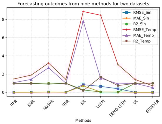
Figure 11.
Comparison of forecasting results from nine methods.
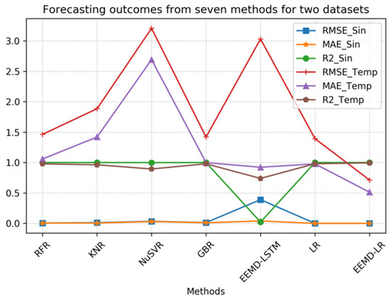
Figure 12.
Comparison of forecasting results from seven methods.
In Table 3, the optimal results are highlighted in bold. EEMD-LR demonstrates superior performance in predicting both sine and temperature data compared to the other methods. Upon meticulous examination of Table 3 and thorough analysis of the experimental values, it is evident that the KR method exhibits the poorest prediction performance for the sine data among the nine methods. Conversely, the remaining eight methods yield satisfactory prediction results, with LR and EEMD-LR displaying the most favorable outcomes. The RMSE and MAE values of KNR, NuSVR, and GBR are all greater than 0.01 but less than 0.03, which indicates that they also have relatively good predictive accuracy but are slightly inferior to LR and EEMD-LR. The MAE and RMSE values of EEMD-LSTM and LSTM are both greater than 0.03 but less than 0.07, which indicates that they have rather average predictive accuracy but significantly poorer performance compared to LR and EEMD-LR. Notably, these five methods excel in forecasting sequences with consistent fluctuations. Figure 13 illustrates the prediction performance of the LR method. The overall predictive efficacy of the LR method is commendable, which is particularly evident when the method is used to forecast 800 consecutive data points. For clarity, only the forecasted results for the 800 successive data points are depicted in the diagrams presented herein.
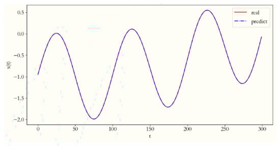
Figure 13.
The LR method’s prediction results for the sine time series.
From Table 3, it is evident that LSTM, EEMD-LSTM, and NuSVR yield notably high MAE and RMSE values for the temperature data, which indicates their poor predictive performance in this regard. Conversely, while NuSVR exhibits relatively high RMSE and MAE values for the sine data, LSTM and EEMD-LSTM do not demonstrate significant discrepancies in this aspect. This suggests that NuSVR, EEMD-LSTM, and LSTM are better suited for forecasting sequences with regular and stable patterns, whereas they may not be as effective for sequences with irregular patterns, as evidenced by the more predictable and stable nature of the sine data.
Upon careful examination of Table 3, it is evident that, although the KR, LSTM, and EEMD-LSTM methods did not, the other five methods demonstrate a favorable predictive performance for sine time-series data. The R2 evaluation index for these five methods exceeds 0.98, which indicates their superior predictive capability for time series that exhibit regular and stable patterns.
Table 4 shows the AIC, SBIC, HQIC, and AICc values for the nine models. The AIC, SBIC, HQIC, and AICc are four commonly used model selection criteria that aim to balance the fit and complexity of models. The AIC selects the optimal model by minimizing information loss, and is suitable for small sample sizes, with smaller AIC values indicating better models. The SBIC imposes a stronger penalty on model complexity, especially for larger sample sizes, with smaller SBIC values indicating better models. The HQIC falls between the AIC and BIC, which makes it suitable for moderate sample sizes. The AICc is a corrected version of the AIC, and is designed to address small sample sizes and reduce the risk of overfitting. Overall, the AIC tends to favor models with a better fit, while the BIC and HQIC place more emphasis on avoiding overfitting, with smaller values typically indicating better models.
Table 4.
Criteria values of nine approaches for two data sets.
Through careful observation of Table 3, it can be seen that the predictive performance of the LSTM and EEMD-LSTM methods is not satisfactory. However, comparing these two algorithms, it can be seen that the EEMD-LSTM method outperforms the LSTM method in terms of the MAE, RMSE, and R2 metrics, which indicates that the EEMD-LSTM outperforms the LSTM in predictive capability.
To facilitate comparison and analysis, we visualized the data. Figure 14 presents the visualization of the data from Table 4, providing a more intuitive way to identify the relationships between them. Through this graphical representation, readers can clearly observe the performance comparison between the proposed method and the other methods. Since the KR and LSTM methods exhibit higher metric values on the temperature sequence, which affect their comparison with other metrics, we excluded these two methods and separately presented the comparison results of the remaining seven methods, which are shown in Figure 15. However, the metric values of the NuSVR and EEMD-LSTM methods are still relatively high, which may hinder the comparison. Therefore, we excluded these two methods as well and separately provided the comparison results for the remaining five methods, as shown in Figure 16. Specifically, the line charts in the figures make it visually easier to distinguish the data, and thus facilitates comparison between the different groups. In observing Figure 14, Figure 15 and Figure 16, it is evident that the proposed method consistently demonstrates lower values across all metrics, which indicates superior performance.
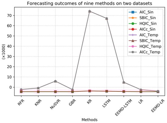
Figure 14.
Comparison of forecasting results of nine methods.
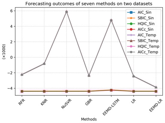
Figure 15.
Comparison of forecasting results of seven methods.
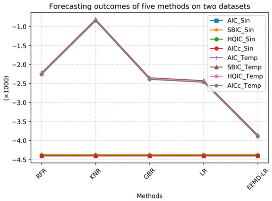
Figure 16.
Comparison of forecasting results of five methods.
5.3. Evaluation of Experimental Outcomes Utilizing Artificial Simulation Data
The proposed method is assessed using artificial simulation experimental data. To ensure the reliability of the experimental results, it is essential to generate a sufficiently long artificial sine simulation time series. As a result, a time series with a length of 10,000 is generated in order to achieve this objective.
Table 3 illustrates our use of nine approaches to predict the sine simulation data. The aim was to assess the forecast accuracy and validity of the proposed approach. The proposed EEMD-LSTM and EEMD-LR methods were applied to predict the sine artificial simulation data prior to scrutinizing the empirical findings of real-world data within the domain. By conducting simulated experiments, the accuracy and efficiency of these two methods can be validated.
Upon analyzing the experimental data in Table 3, it is evident that RFR, KNR, NuSVR, GBR, LR, and the proposed EEMD-LR method exhibit significantly high R2 index values for the temperature data, which indicates their strong forecasting capability for sine data. Additionally, these six methods demonstrate relatively low RMSE and MAE index values for the sine data, which further affirms their efficacy in forecasting sine data. Ultimately, LR and EEMD-LR outperform the others, which confirms the efficiency and accuracy of our proposed EEMD-LR method.
5.4. Evaluation of Experimental Outcomes Utilizing Genuine Data
In our investigation to assess the applicability and efficacy of EEMD-LR, we opt for actual meteorological temperature data for predictive analysis. Temperature, being a component of meteorology, exhibits substantial fluctuations that are largely independent of human influence. Its predictability holds significance for exploring EEMD-LR’s utility in meteorological applications.
The results obtained from the NuSVR experiments outlined in Table 3 demonstrate that it does not perform better than the other methods in predicting data for temperature and sine waves. The consistency and reliability of the temperature and sine series fluctuations suggest that NuSVR is more suitable for predicting such consistent patterns. Despite being a form of support vector regression, NuSVR has been enhanced with improvements that allow for greater flexibility in penalty and loss function selection, which is particularly beneficial for larger sample sizes. Notably, the experimental results in Table 3 indicate that NuSVR’s predictive accuracy does not rank the highest among the tested time-series data.
Table 3 reveals that LSTM struggles in forecasting temperature time-series data but shows marginal improvement with sine time-series data. This is unexpected given the advancements in deep learning algorithms, and suggests that LSTM should excel. However, the experiment’s results imply that the LSTM model construction, parameter configurations, and training iterations may have influenced its underperformance.
In short, our proposed EEMD-LR model achieved RMSE, MAE, and R2 values of 0.000027, 0.000021, and 1.000000, respectively, on the sine simulation time-series data. For the actual temperature time-series data, the model achieved RMSE, MAE, and R2 values of 0.713150, 0.512700, and 0.994749, respectively. The experimental results on these two datasets indicate that the EEMD-LR model demonstrates superior predictive performance compared to alternative methods.
Table 3 presents a comparison of the RMSE evaluation metrics for the predictions of LSTM and EEMD-LSTM on the temperature time series. Notably, the EEMD-LSTM method exhibits superior performance over the standard LSTM approach across both temperature and sine time series. Figure 17 visually depicts the EEMD-LSTM prediction results for the temperature.
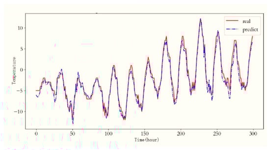
Figure 17.
The EEMD-LSTM method’s prediction results for temperature.
The forecasting results of LR and EEMD-LR for the temperature were evaluated using the MAE and RMSE evaluation indexes, as observed in Table 3. The comparison of the evaluation indexes reveals that EEMD-LR outperforms LR in terms of its RMSE and MAE. Moreover, Figure 18 illustrates the temperature forecasting results achieved by EEMD-LR.
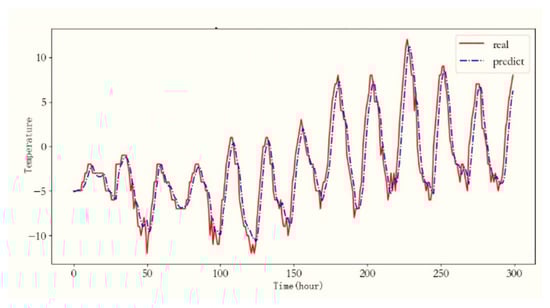
Figure 18.
The EEMD-LR method’s prediction results for temperature.
The results from Table 3 indicate that hybrid methods, such as EEMD-LSTM and EEMD-LR, outperform the initial LSTM and LR approaches across temperature and sine wave datasets. Notably, the EEMD-LR and LR methods demonstrate promising experimental outcomes. This success can likely be attributed to the EEMD algorithm being employed in the hybrid methods, which decomposes the complex sequences into stable and regular sub-sequences, enhancing the models’ predictability and efficacy. To elucidate the EEMD decomposition and wind speed variations, Figure 19 illustrates the sequence and sub-components changes post-EEMD decomposition. The initial sub-graph in Figure 19 depicts the initial sequence shift, while the subsequent sub-graphs are EEMD decomposition sub-graphs, showcasing increased stability, regularity, and simplicity.
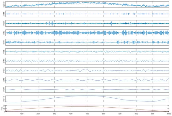
Figure 19.
The temperature time series undergoes EEMD decomposition to produce its decomposed components.
6. Conclusions and Future Work
An innovative hybrid approach, EEMD-LR, is introduced for temperature time-series forecasting, integrating LR and EEMD methodologies. Initially, the EEMD algorithm decomposes the temperature time series into distinct components, each representing a simpler, more regular, and more stable sub-sequence compared to the initial series. Subsequently, the LR method is applied to forecast each sub-component signal. These predicted values are then aggregated to derive the final predictions for the initial temperature series. Two datasets were employed to evaluate the efficacy of our proposed method against nine other techniques, with our proposed method demonstrating a superior predictive performance. While our approach yielded promising results in experimentation, it also exhibited certain limitations, notably in forecasting sequences with abrupt changes.
The field of time-series analysis and forecasting methods has experienced rapid development, yet its effectiveness often falls short of meeting the rigorous demands of practical applications in various fields. Numerous challenges persist, indicating areas for further research and improvement. Despite the efforts outlined in this paper, several avenues remain open for future investigation:
- (1)
- This paper employs the EEMD method to decompose intricate time series, yielding some success. Yet, its predictive efficacy falters when the proposed method is applied to time series with abrupt fluctuations. To address this issue, future endeavors should focus on refining the EEMD method or integrating it with complementary techniques, such as LSTM and transformer methods. This collaborative approach aims to enhance the prediction accuracy for time series characterized by significant variability;
- (2)
- This paper evaluates only nine machine learning techniques for sequence prediction. To facilitate more comprehensive comparative research, future endeavors should explore additional machine learning or deep learning methodologies, for example, models based on LSTM and transformer methodologies. Conducting experiments will enable a thorough understanding of each method’s strengths and weaknesses, aiding in informed selection based on specific practical scenarios;
- (3)
- The experimental outcomes presented in this paper are promising; however, they fall short of our anticipated results. A preliminary analysis of potential factors contributing to this discrepancy is outlined herein, highlighting areas for future investigation and enhancement. Moving forward, our focus will center on refining and amalgamating multiple algorithms to enhance the sequence forecasting efficacy in real-world scenarios. Additionally, leveraging high-performance computing resources, increasing the number of training iterations, and expanding the test dataset size will be paramount to constructing a more robust and applicable learning model.
The EEMD-LR framework faces challenges in highly volatile scenarios (e.g., abrupt regime shifts or extreme events), where EEMD may suffer from residual mode mixing, that compromises its decomposition stability and LR components might inadequately capture transient nonlinear dynamics. For future work, we propose the following: (1) integrating adaptive noise-assisted EEMD variants (e.g., CEEMDAN) to enhance the model’s robustness in high-variability contexts; (2) replacing LR with attention-based deep learning modules (e.g., transformers) to model complex temporal dependencies; (3) developing an uncertainty quantification mechanism for probabilistic forecasts. To strengthen the model’s practical relevance, we will anchor discussions to concrete real-world applications: (a) short-term renewable energy forecasting (e.g., solar/wind generation under erratic weather) and addressing intermittency management for grid stability; (b) high-frequency financial volatility prediction (e.g., cryptocurrency markets) to support algorithmic trading risk control. Case studies from these domains will be prioritized in validation, with methodological advances being explicitly linked to tangible operational impacts.
Author Contributions
Conceptualization, Y.Y. (Yujun Yang) and Y.Y. (Yimei Yang); methodology, H.L.; software, Y.Y. (Yujun Yang); validation, Y.Y. (Yujun Yang), Y.Y. (Yimei Yang) and H.L.; formal analysis, Y.Y. (Yimei Yang); investigation, H.L.; resources, Y.Y. (Yujun Yang); data curation, H.L.; writing—original draft preparation, Y.Y. (Yimei Yang); writing—review and editing, Y.Y. (Yujun Yang) and H.L.; visualization, Y.Y. (Yimei Yang); supervision, Y.Y. (Yujun Yang); project administration, H.L.; funding acquisition, Y.Y. (Yujun Yang) and Y.Y. (Yimei Yang). All authors have read and agreed to the published version of the manuscript.
Funding
This work was partially funded by the Hunan Provincial Natural Science Foundation of China (Grant Nos. 2024JJ7373 and 2024JJ7381), the Key Scientific Research Fund from the Hunan Provincial Department of Education (Grant 22A0548), the Key Laboratory of Intelligent Control Technology for Wuling-Mountain Ecological Agriculture in Hunan Province (Grants ZNKZN2021-09, ZNKZD2023-4, and ZNKZD2024-6).
Data Availability Statement
The data utilized in this paper is freely accessible without any confidentiality constraints. Scholars have the liberty to retrieve it from the UCI ML library (archive.ics.uci.edu/ml/) at no cost.
Acknowledgments
I would like to express my deepest gratitude to my supervisor and paper reviewer for their valuable guidance, insightful suggestions, and constant encouragement throughout this research and the writing of this thesis/dissertation. Their expertise and critical feedback were indispensable in shaping the direction and quality of this work. This work was supported in part by the Key Laboratory of Wuling-Mountain Health Big Data Intelligent Processing and Application in Hunan Province Universities, the Huaihua University Double First-Class initiative Applied Characteristic Discipline of Control Science and Engineering.
Conflicts of Interest
The authors collectively affirm that no conflicts of interest exist among them.
References
- Huang, Y.-P.; Yu, T.-M. The hybrid grey-based models for temperature prediction. IEEE Trans. Syst. Man Cybern. Part B (Cybern.) 1997, 27, 284–292. [Google Scholar] [CrossRef] [PubMed]
- He, Q.; Si, J.; Tylavsky, D. Prediction of top-oil temperature for transformers using neural networks. IEEE Trans. Power Deliv. 2000, 15, 1205–1211. [Google Scholar] [CrossRef]
- Geng, X.; Zou, Y.; Meng, L. Deep Learning and Self-Powered Sensors Enabled Edge Computing Platform for Predicting Microclimate at Urban Blocks. IEEE Sens. J. 2023, 23, 20928–20936. [Google Scholar] [CrossRef]
- Ma, S.; Yao, Q.; Masuda, T.; Higaki, S.; Yoshioka, K.; Arai, S.; Takamatsu, S.; Itoh, T. Development of Noncontact Body Temperature Monitoring and Prediction System for Livestock Cattle. IEEE Sens. J. 2021, 21, 9367–9376. [Google Scholar] [CrossRef]
- Zhang, K.; An, Z.; Gao, X. Time Series Temperature Prediction Model Based on Big Data. In Proceedings of the 2023 IEEE 3rd International Conference on Electronic Technology, Communication and Information (ICETCI), Changchun, China, 26–28 May 2023; pp. 1147–1152. [Google Scholar] [CrossRef]
- Jia, T.; Yang, K.; Peng, Z.; Tang, L.; Duan, H.; Luo, Y. Review on the Change Trend, Attribution Analysis, Retrieval, Simulation, and Prediction of Lake Surface Water Temperature. IEEE J. Sel. Top. Appl. Earth Obs. Remote. Sens. 2022, 15, 6324–6355. [Google Scholar] [CrossRef]
- Wang, H.; Ma, X.; Cui, M.; Dai, Y.; Ye, X.; Lv, X.; Wang, Y. Application of the Informer Long-Term Sequence Model in Agricultural Temperature Prediction. In Proceedings of the 2023 China Automation Congress (CAC), Chongqing, China, 17–19 November 2023; pp. 7122–7127. [Google Scholar] [CrossRef]
- Terliksiz, A.S.; Altylar, D.T. Use Of Deep Neural Networks For Crop Yield Prediction: A Case Study of Soybean Yield in Lauderdale County, Alabama, USA. In Proceedings of the 2019 8th International Conference on Agro-Geoinformatics (Agro-Geoinformatics), Istanbul, Turkey, 16–19 July 2019; pp. 1–4. [Google Scholar] [CrossRef]
- Yu, J.; Sun, C.; Zhao, J.; Ma, L.; Zheng, W.; Xie, Q.; Wei, X. Prediction and control of greenhouse temperature: Methods, applications, and future directions. Comput. Electron. Agric. 2025, 237, 110603. [Google Scholar] [CrossRef]
- Liu, W.; Han, T.; Wang, C.; Zhang, F.; Xu, Z. Predicting indoor temperature of solar green house by machine learning algorithms: A comparative analysis and a practical approach. Smart Agric. Technol. 2025, 12, 101096. [Google Scholar] [CrossRef]
- Li, P.; Luo, Y.; Xia, X.; Shi, W.; Zheng, J.; Liao, Z.; Gao, X.; Chang, R. Advancing photovoltaic panel temperature forecasting: A comparative study of numerical simulation and machine learning in two types of PV power plant. Renew. Energy 2024, 237, 121602. [Google Scholar] [CrossRef]
- Malik, A.; Sudhamsu, G.; Wratch, M.K.; Singh, S.; Sagiraju, S.R.; Mansour, L.; Rai, P.; Ali, R.; Kuriqi, A.; Yadav, K.K. Soil temperature estimation at different depths using machine learning paradigms based on meteorological data. Environ. Monit. Assess. 2024, 197, 104. [Google Scholar] [CrossRef] [PubMed]
- Song, D.; Yang, Y. Temperature prediction of molten iron transporting process based on extended Kalman filter. In Proceedings of the 2018 37th Chinese Control Conference (CCC), Wuhan, China, 25–27 July 2018; pp. 4212–4216. [Google Scholar] [CrossRef]
- Liu, B.; Shen, L.; You, H.; Dong, Y.; Li, J.; Li, Y. Comparison of algorithms for road surface temperature prediction. Int. J. Crowd Sci. 2018, 2, 212–224. [Google Scholar] [CrossRef]
- Wu, P.; He, Y.; Li, Y.; Wang, Y.; Wang, S. Online Prediction of Cutting Temperature Using Self-Adaptive Local Learning and Dynamic CNN. IEEE Trans. Ind. Inform. 2022, 18, 8629–8640. [Google Scholar] [CrossRef]
- Sachan, P.; Bharadwaj, P. Incorporating Uncertainty and Reliability for Battery Temperature Prediction Using Machine Learning Methods. IEEE J. Emerg. Sel. Top. Ind. Electron. 2024, 5, 234–241. [Google Scholar] [CrossRef]
- Hao, H.; Yu, F.; Li, Q. Soil Temperature Prediction Using Convolutional Neural Network Based on Ensemble Empirical Mode Decomposition. IEEE Access 2020, 9, 4084–4096. [Google Scholar] [CrossRef]
- Zhou, H.; Mao, Y.; Song, Z. Probabilistic Forecast of Surface Air Temperature Using Bayesian Model Averaging. Clim. Chang. Res. Lett. 2019, 8, 269–278. [Google Scholar] [CrossRef]
- Li, T.; Zhang, X.; Jiang, Z. What aspect of model performance is the most relevant to skillful future projection on a regional scale. J. Clim. 2024, 37, 1567–1580. [Google Scholar] [CrossRef]
- Zhang, W.Y.; Xie, J.F.; Wan, G.C.; Tong, M.S. Single-step and Multi-step Time Series Prediction for Urban Temperature Based on LSTM Model of TensorFlow. In Proceedings of the 2021 Photonics & Electromagnetics Research Symposium (PIERS), Hangzhou, China, 21 November 2021; pp. 1531–1535. [Google Scholar] [CrossRef]
- Shaowu, D.; Qiangqiang, C.; Hongde, D. Prediction of Exhaust Gas Temperature Margin Based on LSSVR. In Proceedings of the 2019 Chinese Control Conference (CCC), Guangzhou, China, 27–30 July 2019; pp. 6808–6812. [Google Scholar] [CrossRef]
- Long, Y.; Shi, X.; Yang, Y.; Qin, Y.; Lv, J.; Zhang, J. Exhaust Temperature Margin Prediction Based on Time Series Reconstruction. In Proceedings of the 2021 CAA Symposium on Fault Detection, Supervision, and Safety for Technical Processes (SAFEPROCESS), Chengdu, China, 17–18 December 2021; pp. 1–5. [Google Scholar] [CrossRef]
- Zuo, X.; Zhou, X.; Guo, D.; Li, S.; Liu, S.; Xu, C. Ocean Temperature Prediction Based on Stereo Spatial and Temporal 4-D Convolution Model. IEEE Geosci. Remote. Sens. Lett. 2021, 19, 1003405. [Google Scholar] [CrossRef]
- Garai, S.; Paul, R.K.; Yeasin; Paul, A.K. CEEMDAN-Based Hybrid Machine Learning Models for Time Series Forecasting Using MARS Algorithm and PSO-Optimization. Neural Process. Lett. 2024, 56, 92. [Google Scholar] [CrossRef]
- Man, K.; Cao, Z.; Liu, X.; Song, Z.; Liu, R. Predicting TBM Tunnelling Parameters with HHO-LSTM-SVR Model. In Railway Standard Design; Tongfang Zhinan (Beijing) Technology Co., Ltd.: Beijing, China, 2024; pp. 1–12. [Google Scholar] [CrossRef]
- Ondieki, R.; Nyabwanga, R.N.; Waititu, H. Modeling and Forecasting High Frequency Currency Exchange Rates. A Comparative Study of ARIMA, ANN, and Hybrid ARIMA-ANN Models. Asian J. Probab. Stat. 2024, 26, 32–45. [Google Scholar] [CrossRef]
- Ouala, S.; Herzet, C.; Fablet, R. Sea Surface Temperature Prediction and Reconstruction Using Patch-Level Neural Network Representations. In Proceedings of the 2018 IEEE International Geoscience and Remote Sensing Symposium (IGARSS), Valencia, Spain, 22–27 July 2018; pp. 5628–5631. [Google Scholar] [CrossRef]
- Haack, T.; Holt, T.; Tyndall, D.; Granger, B.; Justice, E. Effects of Assimilation of Surface Temperature Data on the Evaporation Duct and Propagation Predictions. In Proceedings of the 2018 USNC-URSI Radio Science Meeting (Joint with AP-S Symposium), Boston, MA, USA, 8–13 July 2018; pp. 103–104. [Google Scholar]
- Geneva, N.; Zabaras, N. Transformers for modeling physical systems. Neural Netw. 2022, 146, 272–289. [Google Scholar] [CrossRef] [PubMed]
- Yang, S.D.; Ali, Z.A.; Wong, B.M. FLUID-GPT (Fast Learning to Understand and Investigate Dynamics with a Generative Pre-Trained Transformer): Efficient Predictions of Particle Trajectories and Erosion. Ind. Eng. Chem. Res. 2023, 62, 15278–15289. [Google Scholar] [CrossRef] [PubMed]
- Huang, N.E.; Shen, Z.; Long, S.R.; Wu, M.C.; Shih, H.H.; Zheng, Q.; Yen, N.-C.; Tung, C.C.; Liu, H.H. The empirical mode decomposition and the Hilbert spectrum for nonlinear and non-stationary time series analysis. In Proceedings of the Royal Society of London. Ser. A Math. Phys. Eng. Sci. 1998, 454, 903–995. [Google Scholar] [CrossRef]
- Wu, Z.; Huang, N.E. Ensemble empirical mode decomposition: A noise-assisted data analysis method. Adv. Adapt. Data Anal. 2009, 1, 1–41. [Google Scholar] [CrossRef]
- Mohguen, O. Noise reduction and QRS detection in ECG signal using EEMD with modified sigmoid thresholding. Biomed. Eng./Biomed. Tech. 2024, 69, 61–78. [Google Scholar] [CrossRef] [PubMed]
- Yin, C.; Zhang, X. The Finger-Based Ecg De-Noising Algorithm Based On Eemd-Md. J. Nanyang Inst. Technol. 2016, 8, 35–39. [Google Scholar] [CrossRef]
- Wang, G.; Lei, W.; Min, Y.; Wan, B.; Li, B.; Wang, Y. Application of an improved EEMD algorithm in high voltage shunt reactor sound signal denoising. Power Syst. Prot. Control 2023, 51, 164–174. [Google Scholar] [CrossRef]
- Yu, H.; Dong, J.; Li, B. Economic insight through an optimized deep learning model for stock market prediction regarding Dow Jones industrial Average index. Expert Syst. Appl. 2025, 291, 128473. [Google Scholar] [CrossRef]
- Xu, T.; Luo, M.; Feng, C.; Wu, Y. A noise suppression method for marine MT data based on SVMD-PSR-MNF. Chin. J. Geophys. 2025, 68, 282–298. [Google Scholar]
- Liu, Z.; Ji, D.; Wang, L. PM2.5 concentration prediction based on EEMD-ALSTM. Sci. Rep. 2024, 14, 12636. [Google Scholar] [CrossRef] [PubMed]
- Wang, Z.; Duan, L.; Shuai, D.; Qiu, T. Research on water environmental indicators prediction method based on EEMD decomposition with CNN-BiLSTM. Sci. Rep. 2024, 14, 1676. [Google Scholar] [CrossRef] [PubMed]
- Zhang, B.; Duan, M.; Sun, Y.; Lyu, Y.; Hou, Y.; Tan, T. Air Quality Index Prediction in Six Major Chinese Urban Agglomerations: A Comparative Study of Single Machine Learning Model, Ensemble Model, and Hybrid Model. Atmosphere 2023, 14, 1478. [Google Scholar] [CrossRef]
- Moualla, L.; Rucci, A.; Naletto, G.; Anantrasirichai, N.; Da Deppo, V. Hybrid GIS-Transformer Approach for Forecasting Sentinel-1 Displacement Time Series. Remote. Sens. 2025, 17, 2382. [Google Scholar] [CrossRef]
- Song, K.-B.; Baek, Y.-S.; Hong, D.H.; Jang, G. Short-term load forecasting for the holidays using fuzzy linear regression method. IEEE Trans. Power Syst. 2005, 20, 96–101. [Google Scholar] [CrossRef]
- Yang, Y.; Liu, J.; Yang, Y.; Xiao, J.; Alkhateeb, A.F. An Efficient Hybrid Method to Predict Wind Speed Based on Linear Regression and VMD. Fractals 2023, 31, 2340135. [Google Scholar] [CrossRef]
- Ma, Q.; Ye, R. Short-Term Prediction of the Intermediate Point Temperature of a Supercritical Unit Based on the EEMD-LSTM Method. Energies 2024, 17, 949. [Google Scholar] [CrossRef]
Disclaimer/Publisher’s Note: The statements, opinions and data contained in all publications are solely those of the individual author(s) and contributor(s) and not of MDPI and/or the editor(s). MDPI and/or the editor(s) disclaim responsibility for any injury to people or property resulting from any ideas, methods, instructions or products referred to in the content. |
© 2025 by the authors. Licensee MDPI, Basel, Switzerland. This article is an open access article distributed under the terms and conditions of the Creative Commons Attribution (CC BY) license (https://creativecommons.org/licenses/by/4.0/).