A Linear Regression Prediction-Based Dynamic Multi-Objective Evolutionary Algorithm with Correlations of Pareto Front Points

Abstract

The Dynamic Multi-objective Optimization Problem (DMOP) is one of the common problem types in academia and industry. The Dynamic Multi-Objective Evolutionary Algorithm (DMOEA) is an effective way for solving DMOPs. Despite the existence of many research works proposing a variety of DMOEAs, the demand for efficient solutions to DMOPs in drastically changing scenarios is still not well met. To this end, this paper is oriented towards DMOEA and innovatively proposes to explore the correlation between different points of the optimal frontier (PF) to improve the accuracy of predicting new PFs for new environments, which is the first attempt, to our best knowledge. Specifically, when the DMOP environment changes, this paper first constructs a spatio-temporal correlation model between various key points of the PF based on the linear regression algorithm; then, based on the constructed model, predicts a new location for each key point in the new environment; subsequently, constructs a sub-population by introducing the Gaussian noise into the predicted location to improve the generalization ability; and then, utilizes the idea of NSGA-II-B to construct another sub-population to further improve the population diversity; finally, combining the previous two sub-populations, re-initializing a new population to adapt to the new environment through a random replacement strategy. The proposed method was evaluated by experiments on the CEC 2018 test suite, and the experimental results show that the proposed method can obtain the optimal MIGD value on six DMOPs and the optimal MHVD value on five DMOPs, compared with six recent research results.

1. Introduction

Dynamic Multi-objective Optimization Problems (DMOPs) have attracted the attention of scientists and developers for decades due to their common appearances in various fields, e.g., logistics [1], disaster management [2], nuclear physics [3], and chemical reaction equipment management [4]. Solving DMOPs is challenging work due to the uncertain change of the actual environmental chaos. The Dynamic Multi-Objective Evolutionary Algorithm (DMOEA) is one of the most efficient ways to overcome this challenge. A DMOEA employs a global search strategy of an evolutionary algorithm (EA) that is inspired by a natural or social law to solve DMOP instances (multi-objective optimization problems) in every steady environmental state (i.e., static multi-objective problems), and tunes searching directions to adapt to changed environments by some reaction/prediction approaches.

It is challenging to design a DMOEA for solving DMOPs. This is mainly because the real world can bring rapid changes to DMOPs, which requires the DMOEA to not only capture the change fast and accurately but also respond to the change in a reasonable way [5]. Therefore, several works have studied responsive approaches for DMOEA to upgrade the search area (the population) based on the predicted movement of the optimal solution set (PS) or the Pareto optimal front (PF) when the environment (the current DMOP instance) is changed. But there are still some issues that existing related works have ignored or not addressed. First, the majority of DMOEAs assume the PS/PF is moving linearly, which falls short of reality. Second, most DMOEAs predict PS/PF movements by only mining the relationship for every single independent variable. These methods infer the new value of a variable from its historical values, and thus do not consider correlations between different variables, even though the phenomenon is common in the real world. Last but not least, to our best knowledge, no existing DMOEA considers the moving interconnectedness of different solutions of PS. Due to the above issues, the current related works can result in inaccurate predicted results, which may lead to bad population updates for the DMOP and degrade the performance of the solution solving.

To overcome the above issues, in this paper, we design a prediction approach based on linear regression (LR) technology to capture correlations between variables and between optimal solutions to accurately learn the movement pattern of PS/PF. To be specific, for the DMOP, by using historical values of all variables jointly, we establish an LR model where the variables in the current environment are the regressand and the variables in the last environment are the regressors. With the LR-based prediction model, we can calculate the variable values in the next environment by the current ones and update the current population based on the predicted variable values to adapt to the new environment. In brief, the contributions of this paper include the following three aspects:

• We propose a PS/PF movement prediction model based on LR to learn correlations between variables and between optimal solutions, which predicts key points of PS in the new environment based on ones of the current PS.
• We design a DMOEA based on the above LR-based prediction model, which updates the population based on the predicted key points of PS when the environment is changed and employs the Non-dominated Sorting Genetic Algorithm II (NSGA-II) to evolve the population when the environment is stable.
• We conduct experiments based on CEC 2018 benchmark DMOPs. The results show that our DMOEA has the best overall performance in solving DMOP, compared with six other up-to-date DMOEAs.

The following contents are organized as follows. The second section illustrates the terminologies that are related to the DMOP and helpful for understanding this paper. The third section presents our proposed DMOEA based on the LR-based prediction model. The fourth section describes the experiment environment for the performance evaluation of the proposed DMOEA. The fifth section shows and analyzes the experiment results. The sixth discusses the existing works related to the DMOEA. The last section concludes the work of this paper.

2. Prerequisite Knowledge

Definition 1 (DMOP (Dynamic  Multi-optimization Problem)).

DMOP is the optimization problem consisting of a series of Multi-optimization Problems (MOPs) or DMOP instances that have multiple objectives. The DMOP instance is changed with the time/environment.

The DMOP can be formulated into Equation (1). $F^{\left(t\right)}=\{f_1^{\left(t\right)},f_2^{\left(t\right)},\dots ,f_{m^{\left(t\right)}}^{\left(t\right)}\}$ is the objectives to be optimized at time t. $m^{\left(t\right)}$ represents the number of optimization objectives at t. Both the objective functions and their number can be changed with the time or the environments. Equations (2) and (3) are equality and inequality constraints, respectively. The constraint functions, $H^{\left(t\right)}$ and $G^{\left(t\right)}$, may be varied with time. $X^{\left(t\right)}=\{x_1^{\left(t\right)},x_2^{\left(t\right)},\dots ,x_{n^{\left(t\right)}}^{\left(t\right)}\}$ includes the independent variables/arguments of the DMOP (objective and constraint functions), with the domain of $D^{\left(t\right)}$. The domain and the number of arguments ($n^{\left(t\right)}$) are also changed with the time. t represents the time that the environment is changed. At this moment, DMOP is changed from one MOP into another. T is the number of environments that DMOP is concerned about. If the DMOP is concerned about the long-term optimization, $T=+\infty$.

$$\begin{array}{c}\hfill minimizing{F}^{\left(t\right)}=\{f_1^{\left(t\right)},f_2^{\left(t\right)},\dots ,f_{m^{\left(t\right)}}^{\left(t\right)}\}\end{array}$$

(1)

subject to

$$\begin{array}{cc}\hfill & H^{\left(t\right)}=0,\hfill \end{array}$$

(2)

$$\begin{array}{cc}\hfill & G^{\left(t\right)}\le 0,\hfill \end{array}$$

(3)

$$\begin{array}{cc}\hfill & X^{\left(t\right)}=\{x_1,x_2,\dots ,x_{n^{\left(t\right)}}\}\in {\mathcal{D}}^{\left(t\right)},\hfill \end{array}$$

(4)

$$\begin{array}{cc}\hfill & t=t_1,t_2,\dots ,t_T.\hfill \end{array}$$

(5)

Definition 2 (Dominating).

For an MOP or a DMOP instance, an available solution dominates another available solution if and only if the first solution does not have a worse value of all objectives than the latter one and has at least one better objective value.

It can be formulated as Equation (6) that the available solution $X_1$ dominates the available solution $X_2$, where F represents the optimization objective functions of the MOP.

$$\begin{array}{c}\hfill X_1\prec X_2:={\forall }_{f\in F}(f\left(X_1\right)\le f\left(X_2\right))\wedge {\exists }_{f\in F}(f\left(X_1\right)<f\left(X_2\right))\end{array}$$

(6)

Definition 3 (Pareto optimal solution set (PS) and Pareto optimal fronts (PFs)).

For an MOP or a DMOP instance, its PS is the set consisting of all available solutions (Pareto optimal solutions) that cannot be dominated by any other solutions. The PF is the set consisting of the objective function values of all Pareto optimal solutions.

PS and PF can be formulated as Equations (7) and (8), respectively, for the MOP with the domain D and the objective function set F.

$$\begin{array}{c}\hfill PS:=\left\{X\right|\neg {\exists }_{X^{\prime }\in D}(X^{\prime }\prec X)\}\end{array}$$

(7)

$$\begin{array}{c}\hfill PF:=\left\{F\right(X\left)\right|X\in PS\}\end{array}$$

(8)

The DMOEA is to find the $PS$ and $PF$ of all DMOP instances for the DMOP.

3. Linear Regression Prediction-Based DMOEA

In this section, to capture various environment change patterns and exploit the inter-correlations of $PF$ points (optimal solutions) of the DMOP, we design an LR-based method to predict positions of some points of $PS$ at the new environment based on their historical positions. In this paper, we consider that the position of each $PF$ point at the next time is decided by that of all $PF$ points in history, as exhibited in Figure 1. Due to the high complexity of predicting all $PF$ points (the entire $PS$), we are concerned about a few key points on $PF$. To be specific, we set key points as 11 statistical points ($10\ast k$-th percentile, $k=0,1,\dots ,10$) and one center point of the $PF$, in this paper. Our proposed method is also compatible with other kinds of key points, e.g., knee points, that we will be concerned about for a better prediction. Below we detail our proposed LR-based method.

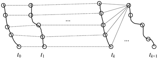
Figure 1. The diagram of exploiting the inter-correlations of key points by the LR-based prediction method for the DMOP. The solid curve is the $PS$ in the time labelled below. The circle represents the key point. The dotted line presents the motion trajectory of the key point. The solid line infers the inter-correlation.

At the beginning of time $t+1$, we have historical $PS$ and $PF$ at all times before t, and need to predict the new $PS$ and $PF$ at $t+1$. Because the manifold of $PF$ is ever-changing for DMOPs in the real world, we focus on the prediction of key points on the $PF$ in this paper, which is a powerful guide in updating the population for the DMOEA to adapt to the environmental changes and is the basic idea employed by almost all existing prediction approaches of DMOEAs. We use $X_k^{\left(t\right)}$ ($k=0,1,\dots ,10$) to represent the $10\ast k$-th percentile of the $PS$ at t, and $X_k^{\left(t\right)}$ ($k=11$) to represent the center of the $PS$ at t, i.e., $X_{11}^{\left(t\right)}={\sum }_{X\in P{S}^{\left(t\right)}}X/\left|P{S}^{\left(t\right)}\right|$. By LR technology, we can establish the relational model of key points between two continuous environments, as Equation (9). $A_k$ ($k\in [0,11]$) and B are the parameters that will be learned by LR, where $A_k^{(t+1)}$ is an $n\times n$ matrix and B is a n dimensional vector. n represents the dimension of the search space of the concerned DMOP. $\widehat{X_k^{(t+1)}}$ represents the estimated/predicted position of $X_k^{(t+1)}$.

$$\begin{array}{c}\hfill \widehat{X_k^{(t+1)}}=\sum _{k\in [0,11]}{A}_k·X_k^{\left(t\right)}+B,k\in [0,11].\end{array}$$

(9)

The samples used for learning the LR model at time $t+1$ include $⟨X^{\left(t^{\prime }\right)},X^{(t^{\prime }+1)}⟩$, $t^{\prime }=0,\dots ,t-1$, which can be easily achieved from the historical $PS$s and $PF$s, and where $X^{\left(t^{\prime }\right)}$ and $X^{(t^{\prime }+1)}$ correspond to $X_k^{\left(t\right)}$ and $\widehat{X_k^{(t+1)}}$ ($k\in [0,11]$) in Equation (9), respectively.

Based on the least-squares method, LR is to learn parameters $A_k^{\left(t\right)}$ and $B^{\left(t\right)}$ to minimize the square error (SE) between predicted values and real values for samples. Thus, learning the LR model is solving the minimization problem (10) for the k-th key point. This optimization problem can be solved by setting the partial derivatives for the parameters to 0. But in such a way, the derived prediction model is easily overfitting. Therefore, L2 regularization is applied to raise the ability to extend the model, and the optimization objective function (loss function) is transformed into Equation (12). $\lambda$ is the regularization coefficient that is generally set to a number less than 0.01 [6,7].

$$\begin{array}{c}\hfill {\mathrm{minimizing}}_{A_k,B}S{E}_k=\sum _{t^{\prime }=1}^t{(\widehat{X_k^{\left(t^{\prime }\right)}}-X_k^{\left(t^{\prime }\right)})}^2\end{array}$$

(10)

$$\begin{array}{c}\hfill =\sum _{t^{\prime }=1}^t{(\sum _{k\in [0,11]}{A}_k·X_k^{(t^{\prime }-1)}+B-X_k^{\left(t^{\prime }\right)})}^2\end{array}$$

(11)

$$\begin{array}{c}\hfill L_k(A_k,B)=S{E}_k+\lambda ·(\sum _{k\in [0,11]}{A}_k^2+B^2)\end{array}$$

(12)

Based on the loss function (12), we can achieve the parameters ($A_k$ ($k\in [0,11]$) and B) by the gradient descent method that updates these parameters step by step by iterative Formulas (13) and (14). $\alpha$ is the learning rate, which is tuned by experiments and is usually set between 0.1 and 0.001 [8]. ${\displaystyle \frac{\partial L_k}{\partial A_k}}$ and ${\displaystyle \frac{\partial L_k}{\partial B}}$ are the partial derivatives of the loss function with respect to the parameters, and can be calculated by Equations (15) and (16).

$$\begin{array}{cc}\hfill & A_k=A_k-\alpha ·{\displaystyle \frac{\partial L_k}{\partial A_k}},k\in [0,11],\hfill \end{array}$$

(13)

$$\begin{array}{cc}\hfill & B=B-\alpha ·{\displaystyle \frac{\partial L_k}{\partial B}}.\hfill \end{array}$$

(14)

$$\begin{array}{cc}\hfill {\displaystyle \frac{\partial L_k}{\partial A_k}}& ={\displaystyle \frac{{\sum }_{t^{\prime }=1}^t{({\sum }_{k\in [0,11]}{A}_k·X_k^{(t^{\prime }-1)}+B-X_k^{\left(t^{\prime }\right)})}^2+\lambda ·({\sum }_{k\in [0,11]}{A}_k^2+B^2)}{\partial A_k}}\hfill \end{array}$$

$$\begin{array}{cc}\hfill & =2·\sum _{t^{\prime }=1}^t({\left(\sum _{k\in [0,11]}{X}_k^{(t^{\prime }-1)}\right)}^T·(\sum _{k\in [0,11]}{A}_k·X_k^{(t^{\prime }-1)}+B-X_k^{\left(t^{\prime }\right)}))+2·\lambda ·A_k,\hfill \end{array}$$

(15)

$$\begin{array}{cc}\hfill {\displaystyle \frac{\partial L_k}{\partial B}}& =2·\sum _{t^{\prime }=1}^t(\sum _{k\in [0,11]}{A}_k·X_k^{(t^{\prime }-1)}+B-X_k^{\left(t^{\prime }\right)})+2·\lambda ·B.\hfill \end{array}$$

(16)

Now, based on the above formula, our proposed LR-based DMOEA can be illustrated by Algorithm 1. At first, the algorithm initializes a population and the environment (lines 1–2 in Algorithm 1). Then, the algorithm evaluates all objective function values for each individual (line 3 in Algorithm 1) and finds $PS$ and $PF$, which consist of individuals that are not dominated by any other individual and their objective function values, respectively (line 4 in Algorithm 1). After this, the algorithm randomly initializes the parameters of the LR model, which will be updated during the DMOP solving process (line 5 in Algorithm 1).

After the above initialization, the algorithm begins to search for solutions for DMOPs by iteratively updating/evolving the population (lines 6–20 in Algorithm 1). There are mainly two kinds of population update methods used in our proposed DMOEA. When the environment is stable (line 15 in Algorithm 1), the population is updated by an evolutionary strategy. In this paper, we focus on the prediction method to adapt to the environmental changes of DMOPs, thus, we simply employ the evolutionary strategy of NSGA-II that is widely used for solving multi-objective problems (lines 15 in Algorithm 1) in this paper. In the future, we will exploit other evolutionary strategies with excellent cooperation with our proposed prediction method to improve the efficiency in solving DMOPs. When the environment is changed (lines 8–13 in Algorithm 1), the DMOEA re-initializes a population with the help of the LR-based prediction method to respond to the change, as described below.

Algorithm 1 LR-based DMOEA

Input:   Objective functions F; domain/solution space D;

Output: $PS$ and $PF$;

1: Randomly initialize a population; 2: Initialize the time or environment; 3: Evaluate the objective function values; 4: Find the current $PS$ and $PF$; 5: Randomly initialize parameters of LR model in Equation (9), $A_k$, B; 6: while not reach termination condition do 7:    Store the last key points, $X_k^{\left(t\right)}$, $k=1,\dots ,11$; 8:    if environment is changed then 9:      Update LR model with stored key points by decreasing gradient algorithm (Algorithm 2); 10:      Predict new positions of key points by the LR model, $\widehat{X_k^{(t+1)}}$; 11:      Build a sub-population with $\widehat{X_k^{(t+1)}}$; 12:      Generate a sub-population with the idea of DNSGA-II-B 13:      Update the population with random replacements 14:    else 15:      Evolve the population and update $PS$ and $PF$ by NSGA-II; 16:    end if 17:    Re-evaluate the objective function values 18:    Update the current $PS$ and $PF$ 19:    Go to the next time tick; 20: end while 21: return$PS$ and $PF$;

Within the environment of a DMOP, the DMOEA first updates parameters of the LR-based prediction model based on the stored locations of $PF$ key points (line 9 in Algorithm 1). The parameter update method for the LR model is outlined in Algorithm 2, and will be talked about later. Then, with the updated LR model, the DMOEA predicts the new locations of key points ($\widehat{X_k^{(t+1)}}$) from their last locations ($X_k^{\left(t\right)}$) by Equation (9) (line 10 in Algorithm 1). Given the predicted new locations, we generate a set of new individuals with the quantity of a certain proportion of the population size, which constitutes a sub-population (line 11 in Algorithm 1). These new individuals are generated by introducing a Gaussian noise into the predicted key points in every dimension, as formulated by Equation (17). P represents the location of a newly generated individual. $N(0,{\sigma }^2)$ is the Gaussian distribution with zero mean and the standard deviation of $\sigma$.

$$P=\widehat{X_k^{(t+1)}}+N(0,{\sigma }^2)$$

(17)

By the introduction of Gaussian noises, the generalization of the prediction method can be improved, as the generated new individuals are more likely to be close to the $PF$ of the new environment, when the predicted locations of key points are near the new $PF$ instead of on it. This is a frequent occurrence because the prediction method is not perfect for precisely predicting the $PF$ movements in the real world.

Next, for improving the population diversity, we employ the population re-initialization method of DNSGA-II-B to generate another sub-population (line 12 in Algorithm 1). When the environment is changed, DNSGA-II-B randomly selects a certain percentage of individuals from the current population, and performs the mutation operator on them to generate new individuals.

Given the above two generated sub-populations, our proposed DMOEA re-initializes the population by randomly replacing part of its individuals with generated ones (line 13 in Algorithm 1).

For new individuals that are generated above by the evolutionary strategy, the prediction method, and the mutation operator of DNSGA-II-B, the proposed DMOEA evaluates their fitness function values (line 17 in Algorithm 1), and updates the current $PS$ and $PF$ (line 18 in Algorithm 1) as some individuals in $PS$ may be dominated by new individuals and there may be new individuals that cannot be dominated by the current $PS$’s members. After this, the proposed DMOEA enters the next tick for the next population re-initialization or evolution (line 19 in Algorithm 1).

The parameters of the LR model used for location predictions of key points are updated at the beginning of every environment change (line 9 in Algorithm 1). In this paper, we employ the decreasing gradient algorithm to learn the LR model based on the historical key points stored in line 7 of Algorithm 1. As illustrated in Algorithm 2, the process of the decreasing gradient algorithm for training the LR model is repeatedly updating the parameters of the LR model by the iterative Formulas (13)–(16) (line 3 in Algorithm 2). This process is repeated until the predefined maximum iteration time is reached or the parameters almost are not updated several times (line 1 in Algorithm 2).

Algorithm 2 LR model training by decreasing gradient algorithm

Input:  Historical key points, $X_k^{\left(t\right)}$, $t=0,1,\dots ,T$, $k=1,\dots ,11$;

initial parameters, $A_k$, $k=1,\dots ,11$, and B;

Output: Updated parameters, $A_k$, B;

1: while not reach termination condition do 2:    for $t=1,\dots ,T$; $k=1,\dots ,11$ do 3:      Update $A_k$ and B by Equations (13)–(16) with $(X_k^{(t-1)},X_k^{\left(t\right)})$; 4:    end for 5: end while 6: return$A_k$, $k=1,\dots ,11$, and B;

4. Experiment Environment

For evaluating the effectiveness and efficiency of our proposed DMOEA, we conducted extensive experiments to compare the performance with six other DMOEAs on the CEC 2018 benchmark test suite [9]. The six benchmark DMOEAs are as follows:

• FL (Forward-Looking) [10] is one of the simplest and most widely used methods for the environmental response of DMOPs. FL assumes that $PF$ moves with a uniform velocity and predicts that the new $PF$ is moving from the current $PF$ with the same step as the last movement (from the last $PF$ to the current $PF$). For the $PF$ center point and every dimension, the moving velocity is $v_k^{\left(t\right)}=x_k^{\left(t\right)}-x_k^{(t-1)}$, and the new position of each $PF$ point is $x_k^{(t+1)}=x_k^{\left(t\right)}+v_k^{\left(t\right)}$.
• FLV (Velocity Forward-Looking) assumes that $PF$ moves with changeable velocity and the velocity is changed with a constant acceleration. Thus, the new position of a key point in a dimension is $x_k^{(t+1)}=x_k^{\left(t\right)}+v_k^{\left(t\right)}+{\displaystyle \frac{1}{2}}·{\left(a_k^{\left(t\right)}\right)}^2$. $v_k^{\left(t\right)}$ is the last moving velocity of the center point. $a_k^{\left(t\right)}$ represents the last moving acceleration of the center point, which is calculated by $a_k^{\left(t\right)}=v_k^{\left(t\right)}-v_k^{(t-1)}$.
• KF (Kalman Filtering-based DMOEA) [11,12] employs the Kalman filtering technology to model the movement of the $PF$ center point.
• SVR (Support Vector Regression-based DMOEA) [13,14] learns a regression model by support vector regression for the $PF$ center point in every dimension based on its historical locations, and predicts the new location by the learned regression model.
• XGB (eXtreme Gradient Boosting-based DMOEA) [15] is similar to SVR except that the regression model is learned by XGB, which is a classical and widely used ensemble learning with boosting technologies.
• RF (Random Forest Regression-based DMOEA) is similar to the above two methods except that the regression model is learned by RF, which is an ensemble learning exploiting the bagging technology.

Due to our focus on the prediction method to adapt to the environmental changes for DMOPs, all of the above DMOEAs exploit NSGA-II as the evolutionary strategy when the environment is stable.

The CEC 2018 benchmark test suite includes 14 DMOPs with varied $PS$ and $PF$ movement patterns. The details of these 14 DMOPs are shown in Table 1, Table 2 and Table 3. In our experiment, we set the environment change to severe by setting the frequency of change and the severity of change to 10 for each DMOP. The number of changes was 30. The number of variables was 10. All of these parameters of DMOPs were set referring to the report that proposes the CEC 2018 test suite [9].

Table 1. The details of DF1-DF6 in the CEC 2018 benchmark suite [9].

Problem	Objectives	PS	PF
DF1	$\begin{array}{cc}& min\left\{\begin{array}{cc}\hfill f_1\left(x\right)& =x_1,\hfill \\ \hfill f_2\left(x\right)& =g\left(x\right)(1-{\left({\displaystyle \frac{x_1}{g\left(x\right)}}\right)}^{H\left(t\right)})\hfill \end{array}\right.\hfill \\ & \begin{array}{cc}\hfill g\left(x\right)& =1+\sum _{i=2}^n{(x_i-G\left(t\right))}^2\hfill \\ \hfill H\left(t\right)& =0.75sin\left(0.5\pi t\right)+1.25\hfill \\ \hfill G\left(t\right)& =|sin(0.5\pi t\left)\right|\hfill \end{array}\hfill \end{array}$	$\begin{array}{cc}& 0\le x_1\le 1\hfill \\ & x_i=G\left(t\right),i=2,\dots ,n\hfill \end{array}$	$\begin{array}{cc}& 0\le f_1\le 1\hfill \\ & f_2=1-f_1^{H\left(t\right)}\hfill \end{array}$
DF2	$\begin{array}{cc}& min\left\{\begin{array}{cc}\hfill f_1\left(x\right)& =x_r,\hfill \\ \hfill f_2\left(x\right)& =g\left(x\right)(1-\sqrt{f_1/g})\hfill \end{array}\right.\hfill \\ & \begin{array}{cc}& g\left(x\right)=1+\sum _{i=\{1,\dots ,n\}\setminus \left\{r\right\}}{(x_i-G\left(t\right))}^2\hfill \\ & G\left(t\right)=|sin(0.5\pi t\left)\right|\hfill \\ & r=1+\lfloor (n-1)G\left(t\right)\rfloor \hfill \end{array}\hfill \end{array}$	$\begin{array}{cc}& 0\le x_r\le 1\hfill \\ & x_{i\ne r}=G\left(t\right),i=1,\dots ,n\hfill \end{array}$	$\begin{array}{cc}& 0\le f_1\le 1\hfill \\ & f_2=1-\sqrt{f_1}\hfill \end{array}$
DF3	$\begin{array}{cc}& min\left\{\begin{array}{cc}\hfill f_1\left(x\right)& =x_1,\hfill \\ \hfill f_2\left(x\right)& =g\left(x\right)(1-{\left({\displaystyle \frac{x_1}{g\left(x\right)}}\right)}^{H\left(t\right)})\hfill \end{array}\right.\hfill \\ & \begin{array}{cc}& g\left(x\right)=1+\sum _{i=2}^n{(x_i-G\left(t\right)-x_1^{H\left(t\right)})}^2\hfill \\ & G\left(t\right)=sin\left(0.5\pi t\right)\hfill \\ & H\left(t\right)=1.5+G\left(t\right)\hfill \end{array}\hfill \end{array}$	$\begin{array}{cc}& 0\le x_1\le 1\hfill \\ & x_i=G\left(t\right)+x_1^{H\left(t\right)},i=2,\dots ,n\hfill \end{array}$	$\begin{array}{cc}& 0\le f_1\le 1\hfill \\ & f_2=1-f_1^{H\left(t\right)}\hfill \end{array}$
DF4	$\begin{array}{cc}& min\left\{\begin{array}{cc}\hfill f_1\left(x\right)& =g\left(x\right)|x_1{-a|}^{H\left(t\right)},\hfill \\ \hfill f_2\left(x\right)& =g\left(x\right)|x_1{-a-b|}^{H\left(t\right)}\hfill \end{array}\right.\hfill \\ & \begin{array}{cc}& g\left(x\right)=1+\sum _{i=2}^n{(x_i-{\displaystyle \frac{a{x}_1^2}{i{c}^2}})}^2\hfill \\ & a=sin\left(0.5\pi t\right)\hfill \\ & b=1+|cos(0.5\pi t\left)\right|\hfill \\ & c=max\left(\right|a|,a+b)\hfill \\ & H\left(t\right)=1.5+a\hfill \end{array}\hfill \end{array}$	$\begin{array}{cc}& a\le x_1\le a+b\hfill \\ & x_i={\displaystyle \frac{a{x}_1^2}{i{c}^2}},i=2,\dots ,n\hfill \end{array}$	$\begin{array}{cc}& 0\le f_1\le b^{H\left(t\right)}\hfill \\ & f_2={(b-f_1^{{\displaystyle \frac{1}{H\left(t\right)}}})}^{H\left(t\right)}\hfill \end{array}$
DF5	$\begin{array}{cc}& min\left\{\begin{array}{cc}\hfill f_1\left(x\right)& =g\left(x\right)(x_1+0.02sin\left(w_t\pi x_1\right)),\hfill \\ \hfill f_2\left(x\right)& =g\left(x\right)(1-x_1+0.02sin\left(w_t\pi x_1\right))\hfill \end{array}\right.\hfill \\ & \begin{array}{cc}& g\left(x\right)=1+\sum _{i=2}^n{(x_i-G\left(t\right))}^2\hfill \\ & G\left(t\right)=sin\left(0.5\pi t\right)\hfill \\ & w_t=\lfloor 10G\left(t\right)\rfloor \hfill \end{array}\hfill \end{array}$	$\begin{array}{cc}& 0\le x_1\le 1\hfill \\ & x_i=G\left(t\right),i=2,\dots ,n\hfill \end{array}$	$\begin{array}{cc}& 0\le f_1\le 1\hfill \\ & f_1+f_2=1\hfill \\ & +0.04sin\left(w_t\pi {\displaystyle \frac{f_1-f_2+1}{2}}\right)\hfill \end{array}$
DF6	$\begin{array}{cc}& min\left\{\begin{array}{cc}\hfill f_1\left(x\right)& =g\left(x\right){(x_1+0.1sin\left(3\pi x_1\right))}^{{\alpha }_t},\hfill \\ \hfill f_2\left(x\right)& =g\left(x\right){(1-x_1+0.1sin\left(3\pi x_1\right))}^{{\alpha }_t}\hfill \end{array}\right.\hfill \\ & \begin{array}{cc}& g\left(x\right)=1+\sum _{i=2}^n\left(\right|G\left(t\right)|y_i^2-10cos\left(2\pi y_i\right)+10)\hfill \\ & G\left(t\right)=sin\left(0.5\pi t\right)\hfill \\ & y_i=x_i-G\left(t\right)\hfill \\ & {\alpha }_t=0.2+2.8\left|G\left(t\right)\right|\hfill \end{array}\hfill \end{array}$	$\begin{array}{cc}& 0\le x_1\le 1\hfill \\ & x_i=G\left(t\right),i=2,\dots ,n\hfill \end{array}$	$\begin{array}{cc}& 0\le f_1\le 1\hfill \\ & f_1^{{\displaystyle \frac{1}{{\alpha }_t}}}+f_2^{{\displaystyle \frac{1}{{\alpha }_t}}}=1\hfill \\ & +0.2sin\left(3\pi {\displaystyle \frac{f_1^{\frac{1}{{\alpha }_t}}-f_2^{\frac{1}{{\alpha }_t}}+1}{2}}\right)\hfill \end{array}$

Table 2. The details of DF7-DF11 in the CEC 2018 benchmark suite [9].

Problem	Objectives	PS	PF
DF7	$\begin{array}{cc}& min\left\{\begin{array}{cc}\hfill f_1\left(x\right)& =g\left(x\right){\displaystyle \frac{1+t}{x_1}},\hfill \\ \hfill f_2\left(x\right)& =g\left(x\right){\displaystyle \frac{x_1}{1+t}}\hfill \end{array}\right.\hfill \\ & \begin{array}{cc}& g\left(x\right)=1+\sum _{i=2}^n{(x_i-{\displaystyle \frac{1}{1+e^{{\alpha }_t(x_1-2.5)}}})}^2\hfill \\ & {\alpha }_t=5cos\left(0.5\pi t\right)\hfill \end{array}\hfill \end{array}$	$\begin{array}{cc}& 0\le x_1\le 1\hfill \\ & x_i={\displaystyle \frac{1}{1+e^{{\alpha }_t(x_1-0.5)}}},\hfill \\ & i=2,\dots ,n\hfill \end{array}$	$\begin{array}{cc}& {\displaystyle \frac{1+t}{4}}\le f_1\le 1+t\hfill \\ & f_2={\displaystyle \frac{1}{f_1}}\hfill \end{array}$
DF8	$\begin{array}{cc}& min\left\{\begin{array}{cc}\hfill f_1\left(x\right)& =g\left(x\right)(x_1+0.1sin\left(3\pi x_1\right)),\hfill \\ \hfill f_2\left(x\right)& =g\left(x\right){(1-x_1+0.1sin\left(3\pi x_1\right))}^{{\alpha }_t}\hfill \end{array}\right.\hfill \\ & \begin{array}{cc}& g\left(x\right)=1+\sum _{i=2}^n{(x_i-{\displaystyle \frac{G\left(t\right)sin\left(4\pi x_1^{{\beta }_t}\right)}{1+\left|G\right(t\left)\right|}})}^2\hfill \\ & {\alpha }_t=2.25+2cos\left(2\pi t\right)\hfill \\ & {\beta }_t=1\hfill \\ & G\left(t\right)=sin\left(0.5\pi t\right)\hfill \end{array}\hfill \end{array}$	$\begin{array}{cc}& 0\le x_1\le 1\hfill \\ & x_i={\displaystyle \frac{G\left(t\right)sin\left(4\pi x_1^{{\beta }_t}\right)}{1+\left|G\right(t\left)\right|}},\hfill \\ & i=2,\dots ,n\hfill \end{array}$	$\begin{array}{cc}& 0\le f_1\le 1\hfill \\ & f_1+f_2^{{\displaystyle \frac{1}{{\alpha }_t}}}=1\hfill \\ & +0.2sin\left(3\pi {\displaystyle \frac{f_1-f_2^{\frac{1}{{\alpha }_t}}+1}{2}}\right)\hfill \end{array}$
DF9	$\begin{array}{cc}& min\left\{\begin{array}{cc}\hfill f_1\left(x\right)& =g\left(x\right)(x_1+max\{0,\hfill \\ & ({\displaystyle \frac{1}{2N_t}}+0.1)sin\left(2N_t\pi x_1\right)\left\}\right),\hfill \\ \hfill f_2\left(x\right)& =g\left(x\right)(1-x_1+max\{0,\hfill \\ & ({\displaystyle \frac{1}{2N_t}}+0.1)sin\left(2N_t\pi x_1\right)\left\}\right)\hfill \end{array}\right.\hfill \\ & \begin{array}{cc}& g\left(x\right)=1+\sum _{i=2}^n{(x_i-cos(4t+x_1+x_{i-1}))}^2\hfill \\ & N_t=1+\lfloor 10|sin\left(0.5\pi t\right)|\rfloor \hfill \end{array}\hfill \end{array}$	$\begin{array}{cc}& x_1\in \bigcup _{i=1}^{N_t}[{\displaystyle \frac{2i-1}{2N_t}},{\displaystyle \frac{i}{N_t}}]\bigcup \left\{0\right\}\hfill \\ & x_i=cos(4t+x_1+x_{i-1}),\hfill \\ & i=2,\dots ,n\hfill \end{array}$	$\begin{array}{cc}& f_1\in \bigcup _{i=1}^{N_t}[{\displaystyle \frac{2i-1}{2N_t}},{\displaystyle \frac{i}{N_t}}]\bigcup \left\{0\right\}\hfill \\ & f_2=1-f_1\hfill \end{array}$
DF10	$\begin{array}{cc}& min\left\{\begin{array}{cc}& f_1\left(x\right)=g\left(x\right){[sin\left(0.5\pi x_1\right)]}^{H\left(t\right)}\hfill \\ & f_2\left(x\right)=g\left(x\right){[sin\left(0.5\pi x_2\right)cos\left(0.5\pi x_1\right)]}^{H\left(t\right)}\hfill \\ & f_3\left(x\right)=g\left(x\right){[cos\left(0.5\pi x_2\right)cos\left(0.5\pi x_1\right)]}^{H\left(t\right)}\hfill \end{array}\right.\hfill \\ & \begin{array}{cc}& g\left(x\right)=1+\sum _{i=3}^n{(x_i-{\displaystyle \frac{sin\left(2\pi (x_1+x_2)\right)}{1+\left|G\right(t\left)\right|}})}^2\hfill \\ & H\left(t\right)=2.25+2cos\left(0.5\pi t\right)\hfill \\ & G\left(t\right)=sin\left(0.5\pi t\right)\hfill \end{array}\hfill \end{array}$	$\begin{array}{cc}& 0\le x_{i=1,2}\le 1\hfill \\ & x_i={\displaystyle \frac{sin\left(2\pi (x_1+x_2)\right)}{1+\left|G\right(t\left)\right|}},\hfill \\ & i=3,\dots ,n\hfill \end{array}$	$\begin{array}{cc}& \sum _{i=1}^3{f}_i^{{\displaystyle \frac{2}{H\left(t\right)}}}=1\hfill \\ & 0\le f_{i=1:3}\le 1\hfill \end{array}$
DF11	$\begin{array}{cc}& min\left\{\begin{array}{cc}& f_1\left(x\right)=g\left(x\right)sin\left(y_1\right)\hfill \\ & f_2\left(x\right)=g\left(x\right)sin\left(y_2\right)cos\left(y_1\right)\hfill \\ & f_3\left(x\right)=g\left(x\right)cos\left(y_2\right)cos\left(y_1\right)\hfill \end{array}\right.\hfill \\ & \begin{array}{cc}& y_{i=1:2}={\displaystyle \frac{\pi }{6}}{G}_t+({\displaystyle \frac{\pi }{2}}-{\displaystyle \frac{\pi }{3}}{G}_t)x_i\hfill \\ & g\left(x\right)=1+G\left(t\right)+\sum _{i=3}^n{(x_i-0.5G\left(t\right)x_1)}^2\hfill \\ & G\left(t\right)=|sin(0.5\pi t\left)\right|\hfill \end{array}\hfill \end{array}$	$\begin{array}{cc}& 0\le x_{i=1,2}\le 1\hfill \\ & x_i=0.5G\left(t\right)x_1,\hfill \\ & i=3,\dots ,n\hfill \end{array}$	$\begin{array}{cc}& \mathrm{a}\mathrm{part}\mathrm{of}\sum _{i=1}^3{f}_i^2={(1+G\left(t\right))}^2\hfill \\ & 0\le f_{i=1:3}\le 1\hfill \end{array}$

Table 3. The details of DF12-DF14 in the CEC 2018 benchmark suite [9].

Problem	Objectives	PS	PF
DF12	$\begin{array}{cc}& min\left\{\begin{array}{cc}& f_1\left(x\right)=g\left(x\right)cos\left(0.5\pi x_1\right)\hfill \\ & cos\left(0.5\pi x_2\right)\hfill \\ & f_2\left(x\right)=g\left(x\right)cos\left(0.5\pi x_1\right)\hfill \\ & sin\left(0.5\pi x_2\right)\hfill \\ & f_3\left(x\right)=g\left(x\right)sin\left(0.5\pi x_1\right)\hfill \end{array}\right.\hfill \\ & \begin{array}{cc}& g\left(x\right)=1+\sum _{i=3}^n{(x_i-sin\left(t{x}_1\right))}^2\hfill \\ & +|\prod _{j=1}^{2}sin(\lfloor k_t(2x_j-r)\rfloor \pi /2)|\hfill \\ & k_t=\lfloor 10sin\left(\pi t\right)\rfloor \hfill \\ & r=1-mod(k_t,2)\hfill \end{array}\hfill \end{array}$	$\begin{array}{cc}& 0\le x_{i=1,2}\le 1\hfill \\ & \prod _{j=1}^{2}mod\left(\right|\lfloor k_t(2x_j-r)\rfloor |,2)=0\hfill \\ & x_i=sin\left(t{x}_1\right),i=3,\dots ,n\hfill \end{array}$	$\begin{array}{cc}& \sum _{i=1}^3{f}_i=1\hfill \\ & 0\le f_{i=1:3}\le 1\hfill \end{array}$
DF13	$\begin{array}{cc}& min\left\{\begin{array}{cc}& f_1\left(x\right)=g\left(x\right){cos}^2\left(0.5\pi x_1\right)\hfill \\ & f_2\left(x\right)=g\left(x\right){cos}^2\left(0.5\pi x_2\right)\hfill \\ & f_3\left(x\right)=g\left(x\right)\sum _{j=1}^2[{sin}^2\left(0.5\pi x_j\right)\hfill \\ & +sin\left(0.5\pi x_j\right){cos}^2\left(p_t\pi x_j\right)]\hfill \end{array}\right.\hfill \\ & \begin{array}{cc}& g\left(x\right)=1+\sum _{i=3}^n{(x_i-G\left(t\right))}^2\hfill \\ & p_t=\lfloor 6G\left(t\right)\rfloor \hfill \\ & G\left(t\right)=sin\left(0.5\pi t\right)\hfill \end{array}\hfill \end{array}$	$\begin{array}{cc}& 0\le x_{i=1,2}\le 1\hfill \\ & x_i=G\left(t\right),i=3,\dots ,n\hfill \end{array}$	$\begin{array}{cc}& \mathrm{DF}13\mathrm{generates}\mathrm{both}\mathrm{continuous}\hfill \\ & \mathrm{and}\mathrm{disconnected}\mathrm{PF}\mathrm{geometries}.\hfill \\ & \mathrm{The}\mathrm{number}\mathrm{of}\mathrm{disconnected}\mathrm{PF}\hfill \\ & \mathrm{segments}\mathrm{varies}\mathrm{over}\mathrm{time}.\hfill \end{array}$
DF14	$\begin{array}{cc}& min\left\{\begin{array}{cc}& f_1\left(x\right)=g\left(x\right)(1-y_1+0.05sin\left(6\pi y_1\right))\hfill \\ & f_2\left(x\right)=g\left(x\right)(1-x_2+0.05sin\left(6\pi x_2\right))\hfill \\ & (y_1+0.05sin\left(6\pi x{y}_1\right))\hfill \\ & f_3\left(x\right)=g\left(x\right)(x_2+0.05sin\left(6\pi x_2\right))\hfill \\ & (y_1+0.05sin\left(6\pi y_1\right))\hfill \end{array}\right.\hfill \\ & \begin{array}{cc}& y_1=0.5+G\left(t\right)(x_1-0.5)\hfill \\ & g\left(x\right)=1+\sum _{i=3}^n{(x_i-G\left(t\right))}^2\hfill \\ & G\left(t\right)=sin\left(0.5\pi t\right)\hfill \end{array}\hfill \end{array}$	$\begin{array}{cc}& 0\le x_{i=1,2}\le 1\hfill \\ & x_i=G\left(t\right),i=3,\dots ,n\hfill \end{array}$	$\begin{array}{cc}& \mathrm{The}\mathrm{dynamics}\mathrm{that}\mathrm{DF}14\mathrm{has}\hfill \\ & \mathrm{is}\mathrm{the}\mathrm{changing}\mathrm{size}\mathrm{and}\hfill \\ & \mathrm{dimension}\mathrm{of}\mathrm{the}\mathrm{PF}. \mathrm{The}\mathrm{PF}\hfill \\ & \mathrm{can}\mathrm{be}\mathrm{degenerated}\mathrm{into}\mathrm{an}1-\mathrm{D}\hfill \\ & \mathrm{manifold}. \mathrm{When}\mathrm{the}\mathrm{PF}\mathrm{is}\mathrm{not}\hfill \\ & \mathrm{degenerate}, \mathrm{the}\mathrm{size}\mathrm{of}\mathrm{the}2-\mathrm{D}\hfill \\ & \mathrm{PF}\mathrm{manifold}\mathrm{changes}\mathrm{over}\mathrm{time}, \hfill \\ & \mathrm{and}\mathrm{the}\mathrm{number}\mathrm{of}\mathrm{knee}\mathrm{regions}\hfill \\ & \mathrm{changes}\mathrm{accordingly}.\hfill \end{array}$

The performance metrics used for evaluating DMOEAs include Mean Inverted Generational Distance (MIGD) [16,17]. Mean Hypervolume Difference (MHVD) [18], and Mean Average Crowding Distance (MACD). MIGD is the average of Inverted Generational Distance (IGD) in all environment cases for solving DMOPs. The calculation of IGD is conducted first by uniformly sampling points from the ideal $PF$ ($P{F}^{\ast }$). Then, for each point on the $P{F}^{\ast }$, it identifies the closest point on the solved $PF$ (obtained by the algorithm), sums all these minimum distances, and then computes their average. A smaller IGD value reflects better alignment between the algorithm’s results and $P{F}^{\ast }$. In summary, MIGD can be calculated by Equations (18) and (19).

$$\begin{array}{cc}\hfill IG{D}_t& ={\displaystyle \frac{{\sum }_{p\in P{F}_t^{\ast }}{min}_{p\in P{F}_t}\left|\right|p^{\ast }-p\left|\right|}{|P{F}_t^{\ast }|}}\hfill \end{array}$$

(18)

$$\begin{array}{cc}\hfill MIGD& ={\displaystyle \frac{1}{T}}·\sum _{t\le T}IG{D}_t\hfill \end{array}$$

(19)

Due to the common unknown ideal $PF$ for real DMOPs, some works use MHVD as a quality metric to quantify the performance of DMOEAs. MHVD is the average value of HVD between $P{F}^{\ast }$ and solved $PF$ for all environments. HVD is the difference between the hypervolumes of $P{F}^{\ast }$ and the solved $PF$. The hypervolume is the Lebesgue measure of the volume dominated by a set of points with respect to a reference point. The reference point can be set to the point that the value is the upper bound of the corresponding objective function in every dimension. Thus, the calculation of MHVD for a solved $PF$ is formulated as Equations (18) and (19), where $HV\left(S\right)$ represents the hypervolume of a point set S.

$$\begin{array}{cc}\hfill HV{D}_t& =HV\left(P{F}_t^{\ast }\right)-HV\left(P{F}_t\right)\hfill \end{array}$$

(20)

$$\begin{array}{cc}\hfill MHVD& ={\displaystyle \frac{1}{T}}·\sum _{t\le T}HV{D}_t\hfill \end{array}$$

(21)

MACD is the time-average of the Average Crowding Distance (ACD) of PF, where the calculation of ACD can refer to [19].

For each of these three above performance metrics, a smaller value indicates better overall algorithm performance in both convergence and distribution characteristics.

In this paper, all experiments were implemented by Python 3.12.2 and Numpy 1.26.4, and run on a personal computer with the Windows 11 HOME operating system, a 14th Gen Intel Core i7-14700(F) CPU, and 16GB of DDR5 memory. Each experiment was repeated 20 times, and the average result is reported below.

5. Experiment Results

Table 4 and Table 5 present the values of various performance metrics achieved by different DMOEAs in solving 14 DMOPs of the CEC 2018 benchmark suite. As shown in the table, we can see that our proposed DMOEA (LR) achieves the best MIGD in six DMOPs, the best MHVD in five DMOPs, and the best MACD in seven DMOPs, and these three numbers are larger than other DMOEAs. This confirms the superior performance of our proposed method for solving DMOPs. The main advantage of our proposed DMOEA is twofold. First, our proposed DMOEA considers predicting the positions of multiple key points instead of only the center point for $PF$. This can adapt to more generalized $PF$ shape changes. Secondly, we try to learn the relationship among different key points of $PF$ by LR, instead of only exploiting the correlation within one signal point (e.g., the center point). Thus, our proposed method achieves the best overall performance.

Table 4. The performance of various DMOEAs in the CEC 2018 benchmark suite (DF1–DF7).

DMOP	Metric		FL	FLS	KF	SVR	XGB	RF	LR-K
DF1	MIGD	avg	0.003358	0.003420	0.005266	0.003673	0.003346	0.003438	0.003625
		rank	2	3	7	6	1	4	5
	MHVD	avg	0.572101	0.572292	0.577866	0.572755	0.571903	0.572468	0.572770
		rank	2	3	7	5	1	4	6
	MACD	avg	0.007299	0.007390	0.007317	0.007334	0.007325	0.007367	0.007164
		rank	2	7	3	5	4	6	1
DF2	MIGD	avg	0.275659	0.279651	0.365038	0.262029	0.273419	0.262997	0.225870
		rank	5	6	7	2	4	3	1
	MHVD	avg	0.500763	0.499969	0.674543	0.498708	0.494868	0.504346	0.225870
		rank	5	4	7	3	2	6	1
	MACD	avg	0.064193	0.060147	0.019380	0.044739	0.052240	0.051317	0.055945
		rank	7	6	1	2	4	3	5
DF3	MIGD	avg	0.687966	0.683465	0.462974	0.645055	0.693014	0.672512	0.676729
		rank	6	5	1	2	7	3	4
	MHVD	avg	0.933143	0.940332	0.688212	0.841667	0.920513	0.923931	0.914939
		rank	6	7	1	2	4	5	3
	MACD	avg	0.370989	0.407731	0.004276	0.525344	0.293931	0.222961	0.363633
		rank	5	6	1	7	3	2	4
DF4	MIGD	avg	0.406392	0.437870	0.335678	0.375508	0.380170	0.392109	0.362976
		rank	6	7	1	3	4	5	2
	MHVD	avg	0.252013	0.245072	0.270142	0.252262	0.237715	0.240964	0.240490
		rank	5	4	7	6	1	3	2
	MACD	avg	0.022482	0.023898	0.022069	0.025366	0.024168	0.023206	0.027455
		rank	2	4	1	6	5	3	7
DF5	MIGD	avg	0.23000	0.25843	0.38152	0.43196	0.36711	0.39712	0.21538
		rank	2	3	5	7	4	6	1
	MHVD	avg	0.283683	0.294900	0.167764	0.293118	0.288968	0.294741	0.290883
		rank	2	7	1	5	3	6	4
	MACD	avg	0.054019	0.043026	0.043663	0.039721	0.058067	0.050178	0.052056
		rank	6	2	3	1	7	4	5
DF6	MIGD	avg	9.558898	9.017478	10.229062	10.218425	10.380135	8.760323	8.828903
		rank	4	3	6	5	7	1	2
	MHVD	avg	0.168647	0.171978	0.252734	0.216913	0.244878	0.268537	0.157827
		rank	2	3	6	4	5	7	1
	MACD	avg	0.107531	0.174019	0.155406	0.114493	0.112718	0.164290	0.106967
		rank	2	7	5	4	3	6	1
DF7	MIGD	avg	0.409614	0.413110	0.299303	0.437491	0.406960	0.388607	0.365055
		rank	5	6	1	7	4	3	2
	MHVD	avg	0.818215	0.820505	0.735557	0.819941	0.823691	0.796808	0.800441
		rank	4	6	1	5	7	2	3
	MACD	avg	0.043981	0.049198	0.051162	0.051297	0.044731	0.049661	0.043827
		rank	2	4	6	7	3	5	1

Table 5. The performance of various DMOEAs in the CEC 2018 benchmark suite (DF8–DF14).

DMOP	Metric		FL	FLS	KF	SVR	XGB	RF	LR-K
DF8	MIGD	avg	0.219790	0.196833	0.259083	0.200351	0.198518	0.198284	0.205540
		rank	6	1	7	4	3	2	5
	MHVD	avg	0.477825	0.436577	0.636385	0.478566	0.474214	0.460388	0.460648
		rank	5	1	7	6	4	2	3
	MACD	avg	0.057704	0.040442	0.035920	0.055057	0.064762	0.030323	0.036103
		rank	6	4	2	5	7	1	3
DF9	MIGD	avg	1.204431	1.178037	1.170227	1.289633	1.382307	1.314454	0.939267
		rank	4	3	2	5	7	6	1
	MHVD	avg	0.308318	0.312206	0.311153	0.324605	0.330248	0.341792	0.275004
		rank	2	4	3	5	6	7	1
	MACD	avg	0.079905	0.092809	0.074488	0.080954	0.089617	0.083600	0.073592
		rank	3	7	2	4	6	5	1
DF10	MIGD	avg	0.355890	0.388526	0.426804	0.394865	0.387404	0.353523	0.311121
		rank	3	5	7	6	4	2	1
	MHVD	avg	0.239955	0.235306	0.308834	0.249693	0.228401	0.212611	0.202771
		rank	5	4	7	6	3	2	1
	MACD	avg	0.021100	0.015084	0.023202	0.018040	0.018209	0.018609	0.016982
		rank	6	1	7	3	4	5	2
DF11	MIGD	avg	11.79304	11.82225	11.85004	11.83362	11.80916	11.80096	11.84234
		rank	1	4	7	5	3	2	6
	MHVD	avg	0.721769	0.716260	0.747332	0.721126	0.720429	0.715592	0.718209
		rank	6	2	7	5	4	1	3
	MACD	avg	0.010971	0.012517	0.010849	0.011759	0.012525	0.011470	0.012211
		rank	2	6	1	4	7	3	5
DF12	MIGD	avg	0.529298	0.519937	0.554105	0.524483	0.510533	0.585771	0.549777
		rank	4	2	6	3	1	7	5
	MHVD	avg	0.204682	0.195807	0.374341	0.207880	0.191020	0.195776	0.205893
		rank	4	3	7	6	1	2	5
	MACD	avg	0.015886	0.017159	0.016816	0.018120	0.017619	0.015821	0.015708
		rank	3	5	4	7	6	2	1
DF13	MIGD	avg	0.162425	0.146274	0.148225	0.172216	0.162629	0.156787	0.143541
		rank	5	2	3	7	6	4	1
	MHVD	avg	1.143186	1.096158	1.341601	1.262261	1.286514	1.262658	0.905825
		rank	3	2	7	4	6	5	1
	MACD	avg	0.015787	0.015404	0.016102	0.016372	0.015820	0.015770	0.014676
		rank	4	2	6	7	5	3	1
DF14	MIGD	avg	0.324704	0.368483	0.425004	0.506701	0.432308	0.480623	0.286369
		rank	2	3	4	7	5	6	1
	MHVD	avg	0.276849	0.294728	0.277859	0.309170	0.310194	0.317478	0.301353
		rank	1	3	2	5	6	7	4
	MACD	avg	0.028267	0.029866	0.025451	0.029066	0.027354	0.028219	0.024529
		rank	5	7	2	6	3	4	1
Count (rank = 1)		MIGD	1	1	3	0	2	1	6
		MHVD	1	1	3	0	3	1	5
		MACD	0	1	4	1	0	1	7
		Total	2	3	10	1	5	3	18

There are mainly two situations in which our proposed method achieves a relatively poor performance. The first one is when $PF$ has almost a parallel motion overall, such as DF1. In such a case, DMOEAs that predict the $PF$ based on only its center point may achieve better performance than our proposed method that employs the correlation of multiple key points. This is because correlation learning introduces more complex patterns of environmental changes, which is helpful for DMOPs with irregular changes, but may not accurately capture simple rules.

Another situation where our proposed method does not achieve the best performance is when the environment changes are too complex to predict. In this case, no prediction method achieves a good performance, while the simplest method may achieve the best performance. For example, FL achieves the best MIGD for DF11 and the best MHVD for DF14.

Next, we illustrate the stability of our proposed method based on the box plots of performance metric values achieved by various algorithms. To avoid overly lengthy content, we took the MIGD metric and DF1-DF3 as case studies, as shown in Figure 2, for the following two reasons. First, the results are similar between different performance metrics. Second, these three cases include three scenes where the ranks of our algorithms are low, the best, and high, respectively. As we can see from Figure 2, the interquartile range achieved by our algorithm has a similar rank to the average value in each case. Additionally, the box plots achieved by our algorithm have no outliers. Therefore, our algorithm has a stable performance in solving DMOPs.

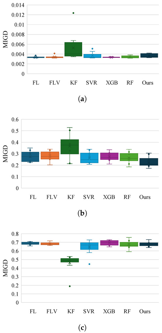
Figure 2. The box plots of MIGD metric values achieved by various algorithms in solving DF1–DF3. (a) DF1. (b) DF2. (c) DF3.

6. Related Works

The basic idea of a DMOEA is predicting the change patterns of DMOP environments ($PS$ and $PF$) and generating new individuals for population re-initialization to adapt to the new environment when it is changed. Therefore, there are several related works aiming at designing accurate prediction methods for DMOEAs.

Zhang et al. [20] first divided the population into several sub-populations, and calculated the accelerations of the center points for these sub-populations. Then, they calculated the velocity for each sub-population based on its center point’s acceleration, and re-initialized a population by adding the velocity and each individual for every sub-population. Wang et al. [21] first detected the intensity of the environmental change based on the difference between the objective function values of a small proportion of the population in two consecutive environments. Then, based on the detection result, they predicted new individuals by a multi-objective particle swarm optimization algorithm [22] with adapted particle velocity updates and the strength Pareto evolutionary algorithm [23]. Different from most works that employed the first-order difference strategy, where the trajectory of moving solutions is decreased by the centroid of $PS$, Zhang et al. [24] proposed to use the second-order difference method that considered both $PF$ and $PS$. The new $PS$ center is decided by the joint trajectories of $PF$ and $PS$ by mapping them into a new two-dimensional space.

To overcome the limitation of most DMOEAs that only rely on predictions from adjacent environments, resulting in a new population adapting to the new environment not well, Zhang et al. [25] used the Fuzzy C-Means clustering algorithm to cluster all historical PSs, and then divided the clusters into high-quality and low-quality sets based on their center points. With the cluster result, a Support Vector Machine (SVM) classifier was trained to predict whether a new solution is high quality. The re-initialized population consists of randomly generated individuals that are predicted to be high quality by the SVM classifier and Gaussian-mutated initial individuals. Ge et al. [26] employed correlation alignment and a probabilistic annotation classifier to get high-quality solutions from the current population and randomly generated individuals in the new environment. Based on the dynamic change pattern of elite individuals, which is learned by correlation analysis and a denoising autoencoder, this work identified the parents of current elite solutions, and then used a denoising autoencoder to transfer the change pattern to new environments. This step predicted a set of individuals based on current elitist solutions and the last $PS$. Individuals predicted by these two steps form the re-initialized population for the new environment.

In this paper, to make better predictions by capturing different moving styles of $PF$ for the DMOP, we try to establish a relation model of different points on $PF$. This is the first attempt to introduce the inter-correlations between the movement of different points into the DMOEA, to our best knowledge.

7. Conclusions

In this paper, we focus on the prediction method for DMOEA to adapt to the environmental changes of DMOPs. We proposed to exploit the correlations of different points in $PF$. For this purpose, we use LR to learn a relationship model from the historical locations of all key points to the current location of one key point, and predict the next location by using the learned model for each key point. Then, by introducing Gaussian noise, a certain proportion of individuals is generated for re-initiating the population when the environment is changed. Extensive experiments on the CEC 2018 benchmark suite are conducted to verify the efficiency and effectiveness of our proposed method, and results show that our proposed method provides solutions with better accuracy and diversity compared with six state-of-the-art related works.

In this work, there are two directions that we will study to improve the performance of DMOEAs. The first one is to exploit more powerful machine learning technologies for training more accurate relationship models, so that DMOEAs can be better and faster at adapting to new environments. The second is that we will seek evolutionary strategies with a more balanced ability of exploration versus exploitation to help DMOEAs search for high-quality solutions quickly, referring to newly proposed improvements, e.g., clustering-based selection [27] and surrogate assist [28].

References

- Zhao, Y.; Shen, X.; Ge, Z. A Knowledge-Guided Multi-Objective Shuffled Frog Leaping Algorithm for Dynamic Multi-Depot Multi-Trip Vehicle Routing Problem. Symmetry 2024, 16, 697. [Google Scholar] [CrossRef]
- Geng, S.; Hou, H.; Zhou, Z. A dynamic multi-objective model for emergency shelter relief system design integrating the supply and demand sides. Nat. Hazards 2024, 120, 2379–2402. [Google Scholar] [CrossRef]
- Zhang, Z.; Guo, Y.; Tao, Q. Dynamic multi-objective path-order planning research in nuclear power plant decommissioning based on NSGA-II. Ann. Nucl. Energy 2024, 199, 110369. [Google Scholar] [CrossRef]
- Zhang, X.; Zhang, G.; Zhang, D.; Zhang, L. Dynamic Multi-Objective Optimization in Brazier-Type Gasification and Carbonization Furnace. Materials 2023, 16, 1164. [Google Scholar] [CrossRef] [PubMed]
- Jiang, S.; Zou, J.; Yang, S.; Yao, X. Evolutionary Dynamic Multi-objective Optimisation: A Survey. ACM Comput. Surv. 2023, 55, 47. [Google Scholar] [CrossRef]
- Qiu, X.; Chen, Y.; Lin, Y.; Huang, B. Enhancing Stability in Real Nor-Flash Compute-In-Memory Chips: A Narrowing Output Range Approach Using Elastic Net Regularization. In Proceedings of the 2024 International Symposium on Integrated Circuit Design and Integrated Systems (ICDIS’24), Xiamen, China, 22–24 November 2024; pp. 31–40. [Google Scholar] [CrossRef]
- Vultureanu-Albişi, A.; Bădică, C. The Model of Regularization Coefficient in Polynomial Regression for Modelling the Spread of COVID-19 in Romania. In Proceedings of the 2022 23rd International Carpathian Control Conference (ICCC), Sinaia, Romania, 29 May–1 June 2022; pp. 94–100. [Google Scholar] [CrossRef]
- Goodfellow, I.; Bengio, Y.; Courville, A. Deep Learning; MIT Press: Cambridge, MA, USA, 2016; Available online: http://www.deeplearningbook.org (accessed on 17 June 2025).
- Jiang, S.; Yang, S.; Yao, X.; Tan, K.; Kaiser, M.; Krasnogor, N. Benchmark Problems for CEC’2018 Competition on Dynamic Multiobjective Optimisation. 2017. Available online: http://homepages.cs.ncl.ac.uk/shouyong.jiang/cec2018/CEC2018_Tech_Rep_DMOP.pdf (accessed on 17 June 2025).
- Li, Q.; Liu, X.; Wang, F.; Wang, S.; Zhang, P.; Wu, X. A framework based on generational and environmental response strategies for dynamic multi-objective optimization. Appl. Soft Comput. 2024, 152, 111114. [Google Scholar] [CrossRef]
- Muruganantham, A.; Tan, K.C.; Vadakkepat, P. Evolutionary Dynamic Multiobjective Optimization Via Kalman Filter Prediction. IEEE Trans. Cybern. 2016, 46, 2862–2873. [Google Scholar] [CrossRef]
- Chen, M.; Ma, Y. Dynamic multi-objective evolutionary algorithm with center point prediction strategy using ensemble Kalman filter. Soft Comput. 2021, 25, 5003–5019. [Google Scholar] [CrossRef]
- Fang, Z.; Li, H.; Hu, L.; Zeng, N. A learnable population filter for dynamic multi-objective optimization. Neurocomputing 2024, 574, 127241. [Google Scholar] [CrossRef]
- Sun, H.; Ma, X.; Hu, Z.; Yang, J.; Cui, H. A two stages prediction strategy for evolutionary dynamic multi-objective optimization. Appl. Intell. 2023, 53, 1115–1131. [Google Scholar] [CrossRef]
- Gao, K.; Xu, L. Novel strategies based on a gradient boosting regression tree predictor for dynamic multi-objective optimization. Expert Syst. Appl. 2024, 237, 121532. [Google Scholar] [CrossRef]
- Ishibuchi, H.; Masuda, H.; Tanigaki, Y.; Nojima, Y. Modified Distance Calculation in Generational Distance and Inverted Generational Distance. In Proceedings of the Evolutionary Multi-Criterion Optimization, Guimarães, Portugal, 29 March–1 April 2015; pp. 110–125. [Google Scholar]
- Yang, Y.; Ma, Y.; Wang, P.; Xu, Y.; Wang, M. A dynamic multi-objective evolutionary algorithm based on two-stage dimensionality reduction and a region Gauss adaptation prediction strategy. Appl. Soft Comput. 2023, 142, 110333. [Google Scholar] [CrossRef]
- Zheng, J.; Zhang, B.; Zou, J.; Yang, S.; Hu, Y. A dynamic multi-objective evolutionary algorithm based on Niche prediction strategy. Appl. Soft Comput. 2023, 142, 110359. [Google Scholar] [CrossRef]
- Deb, K.; Pratap, A.; Agarwal, S.; Meyarivan, T. A fast and elitist multiobjective genetic algorithm: NSGA-II. IEEE Trans. Evol. Comput. 2002, 6, 182–197. [Google Scholar] [CrossRef]
- Zhang, J.; Qu, S.; Zhang, Z.; Cheng, S.; Li, M.; Bi, Y. An acceleration-based prediction strategy for dynamic multi-objective optimization. Soft Comput. 2024, 28, 1215–1228. [Google Scholar] [CrossRef]
- Wang, Y.; Ma, Y.; Li, Q.; Zhao, Y. A dynamic multi-objective optimization evolutionary algorithm based on classification of environmental change intensity and collaborative prediction strategy. J. Supercomput. 2025, 81, 54. [Google Scholar] [CrossRef]
- Coello, C.; Pulido, G.; Lechuga, M. Handling multiple objectives with particle swarm optimization. IEEE Trans. Evol. Comput. 2004, 8, 256–279. [Google Scholar] [CrossRef]
- Zitzler, E.; Laumanns, M.; Thiele, L. SPEA2: Improving the Strength Pareto Evolutionary Algorithm; ETH Zurich: Zurich, Switzerland, 2001. [Google Scholar]
- Zhang, H.; Wang, G.G.; Dong, J.; Gandomi, A.H. Improved NSGA-III with Second-Order Difference Random Strategy for Dynamic Multi-Objective Optimization. Processes 2021, 9, 911. [Google Scholar] [CrossRef]
- Zhang, T.; Tao, Q.; Yu, L.; Yi, H.; Chen, J. A new prediction strategy for dynamic multi-objective optimization using hybrid Fuzzy C-Means and support vector machine. Neurocomputing 2025, 621, 129291. [Google Scholar] [CrossRef]
- Ge, F.; Zhao, X.; Chen, D.; Shen, L.; Liu, H. A dynamic multi-objective optimization algorithm based on probability-driven prediction and correlation-guided individual transfer. J. Supercomput. 2025, 81, 348. [Google Scholar] [CrossRef]
- Akopov, A.S. An Improved Parallel Biobjective Hybrid Real-Coded Genetic Algorithm with Clustering-Based Selection. Cybern. Inf. Technol. 2024, 24, 32–49. [Google Scholar] [CrossRef]
- Díaz-Manríquez, A.; Toscano, G.; Barron-Zambrano, J.H.; Tello-Leal, E. A Review of Surrogate Assisted Multiobjective Evolutionary Algorithms. Comput. Intell. Neurosci. 2016, 2016, 9420460. [Google Scholar] [CrossRef] [PubMed]
Disclaimer/Publisher’s Note: The statements, opinions and data contained in all publications are solely those of the individual author(s) and contributor(s) and not of MDPI and/or the editor(s). MDPI and/or the editor(s) disclaim responsibility for any injury to people or property resulting from any ideas, methods, instructions or products referred to in the content. |
© 2025 by the authors. Licensee MDPI, Basel, Switzerland. This article is an open access article distributed under the terms and conditions of the Creative Commons Attribution (CC BY) license (https://creativecommons.org/licenses/by/4.0/).