Scalable Resource Provisioning Framework for Fog Computing Using LLM-Guided Q-Learning Approach

Abstract

Fog computing is one of the growing distributed computing platforms incorporated by Industries today as it performs real-time data analysis closer to the edge of the IoT network. It offers cloud capabilities at the edge of the fog networks through improved efficiency and flexibility. As the demands of Internet of Things (IoT) devices keep varying, it is important to rapidly modify the resource allocation policies to satisfy them. Constant fluctuation of the demands leads to over or under provisioning of resources. The computing capability of the fog nodes is small, and hence there is a necessity to develop resource provisioning policies that reduce the delay and bandwidth consumption. In this paper, a novel large language model (LLM)-guided Q-learning framework is designed and developed. The uncertainty in the fog environment in terms of delay incurred, bandwidth usage, and heterogeneity of fog nodes is represented using the LLM model. The reward shaping of a Q-learning agent is enriched by considering the heuristic value of the LLM model. The experimental results ensure that the proposed framework is good with respect to processing delay, energy consumption, load balancing, and service level agreement violation under a finite and infinite fog computing environment. The results are further validated through the expected value analysis statistical methodology.

1. Introduction

Fog computing is an extended part of cloud computing that uses edge devices to carry out computation, communication, and storage. The data, applications, and resources of the cloud are moved closer to the end users. Even the workload generated by IoT devices is decentralized to reduce the latency incurred and to increase the efficiency of operation. The fog computing market is increasing as there is a need for developing low-latency solutions and real-time processing of applications. The market size of fog computing at the global level is expected to reach USD 12,206 million by 2033. The growing market size is because of the increasing number of IoT devices which demand the need to process and analyze data closer to the source of the applications [1,2].

The distributed nature of fog computing poses significant challenges with respect to accessibility, resource provisioning, security, privacy, load balancing, and many other factors. Fog computing extends support for millions of IoT requests, and their demands are heterogeneous and stringent in nature. Resource provisioning is one of the prominent challenges in a fog environment as the user exhibits high demands for resources like bandwidth, throughput, response time, and availability. Improper provisioning of resources has a greater impact on performance by increasing the latency and also causes inefficiency for services within the fog network. Hence, there is a need to formulate a proper resource management policy for a better user experience [3,4].

Q learning is a basic form of reinforcement learning that determines the optimal action policy for a finite Markov Decision Process through interaction with the environment in repetition. In a computing environment with a large state space, the learning process is slow and often requires several episodes of training and ends up with suboptimal solutions. With the increase in the state space, the size of the Q-table keeps growing, which leads to high memory usage and results in inefficient exploitation of the state space. The success of the Q-learning model is determined by the reward function, which reflects the ability of the Q-learning agent to reach the goal state with minimum episodes of training. Proper reward shaping enhances the effectiveness of the Q-learning algorithm [5,6].

A typical large language model (LLM) represents a world model for planning and control operation. It enables autonomous state exploration and directly outputs rewards and states. LLMs are lightweight in nature, which makes them suitable for deployment in fog environments. The models are further optimized to reduce the size of the model and speed up the arrival of inference using the Generative Pre-trained Transformer Quantized (GPTQ) method. The use of edge accelerators like NVIDIA JavaScript Object Notation (JSON) and a Tensor Processing Unit (TPU) helps in efficient execution of LLM models at edge devices by preserving the privacy of the data. The LLM-guided Q-learning algorithm uses the LLM’s action probability as a heuristic value to influence the Q function. Here, the LLM model is employed to guide the Q-learning agent for reward shaping using the heuristic value. It modulates the Q-value function by implicitly inducing the desired resource provisioning policy in it. The reshaped Q function prevents the over and under estimation of the policies and converges to an optimal solution [7,8].

In this paper, a novel LLM-guided Q-learning framework is designed to address the resource provisioning problem. The action bonus form of the heuristic, i.e., maximum entropy, is generated by the LLM model, which encourages exploration of the large state space fog environment. The heuristic value generated by the LLM provides navigation guidance to a Q-learning agent at every iteration step, which results in the formulation of the desired policy in the upcoming iterations of training. The expected value analysis under a finite and infinite fog environment is performed towards objective functions to arrive at the desired resource provisioning policies [9,10].

The objectives of this paper are as follows:

• Mathematical representation of the fog computing system model and objective functions considered for evaluation purposes.
• Design of a novel framework for resource provisioning using an LLM-guided Q-learning model.
• Illustration of algorithms for each of the components in the LLM-guided Q-learning model.
• Expected value analysis of the proposed framework in a finite and infinite fog environment.
• Simulation of the proposed framework using the iFogSim 3.3 simulator by considering the ChatGPT classic model as a large language model and synthetic workload.

The remaining sections of the paper are organized as follows: Section 2 deals with the related work, Section 3 presents the system model, Section 4 discusses the proposed framework, Section 5 presents expected value analysis of the proposed framework under a finite and infinite fog environment, Section 6 discusses the results, and finally Section 7 arrives at the conclusion.

2. Related Work

In this section, some of the potential recent papers on scalable resource provisioning for fog computing are discussed and their limitations are identified.

Najwa et al. discuss a Quality of Service (QoS) aware resource provisioning approach for fog environments. Two crucial challenges are involved in designing the resource provisioning framework for maximizing the throughput and minimizing the latency [11]. Low latency applications prefer the fog paradigm, as delay and congestion in service are overcome by bringing the cloud services to the edge of the network. An application placement strategy based on a greedy approach was designed to minimize the latency of IoT applications. Here, the incoming requests are distributed among the fog nodes using a greedy edge placement strategy. The approach is composed of two stages: the first stage is proper placement of requests across fog nodes to satisfy the high QoS needs of the real-time applications; and the second stage is depth-first search logic, which is used to identify the fog nodes that satisfy the bandwidth requirement of the incoming application requests. Each of the incoming requests is assigned priority during the placement process according to its processing requirements. The requests having higher processing requirements are sent to the nearest IoT devices for servicing. Here, resource provisioning latency requirement of the incoming requests is addressed. The evaluation was performed by considering the Distributed Camera Network (DCN) as a benchmark application. The DCN applications are mounted onto the fog nodes using a variable-sized tree network topology. From the results it was inferred that the end-to-end delay is minimized. However, the chances of getting stuck in an infinite loop is greater as the approach does not keep track of the visited fog nodes during placement of the application requests.

Masoumeh et al. present an autonomic approach to efficiently allocate the resources for IoT requests [12]. The IoT requests experience heavy workload variation with respect to time, which needs to be addressed to prevent over/under provisioning of the resources. A Bayesian learning-inspired automated computing model was designed to make dynamic scaling decisions about whether to increase/decrease the resources for fog nodes. The Bayesian learning model is dependent on conditional probability for deciding the occurrence or non-occurrence of the event. A time-series prediction model was used to perform planning and analysis of the control loop. The autonomic system is composed of four major components: monitor, analyze, plan, and execute (MAPE). The MAPE module was further enriched with a knowledge database (MAPE-k). The MAPE-k computing model was introduced by IBM and executes MAPE modules automatically to calculate the number of fog nodes to be deployed for executing the IoT services. The time-series model is used to predict the future demand for resources. A three-tier fog computing architecture was considered for implementation purposes comprising a IoT device tier, fog tier, and cloud tier. The proposed MAPE-k module sits at the fog tier, which does automatic resource provisioning. The MAPE-k control module is executed in a loop through several iterations at regular intervals of time to allocate the fog nodes as per the dynamic changes in the IoT services workloads. However, the practical applicability of the approach is limited, as the Bayesian learning expects the computing environment to be static. In a static computing environment, sufficient information on the computing environment is known in advance; however, the fog environment is totally unpredictable, complex, heterogeneous, and highly dynamic in nature.

Nguyen et al. present an elastic form of resource provisioning framework for container-based applications in the fog computing paradigm [13]. Kubernetes is one of the most widely used orchestration platforms for container-based applications. The framework is designed to execute over the Kubernetes computing platform to deliver resources in real-time. The ongoing traffic information is gathered in real-time and resources are allocated in proportion to the traffic distribution. Here, the Kubernetes platform is used for the purpose of orchestration, and the IoT applications are kept in the form of a container and deployed inside the fog nodes. Fog nodes situated in the nearby vicinity operate together in the form of a cluster. Two important limitations of traditional Kubernetes are that it does not consider network traffic status for application scheduling and it does not monitor the changing popularity of the applications over time. Here, the real-time traffic information is gathered at frequent time intervals. Affinity-based priority rules are formulated that specify the intended location for the fog nodes. The relocation decisions about the fog nodes are made as per the formulated affinity-based priority rules. To determine the best-fit node for the application, several factors are considered, including the health of the node, node affinity, location of the node, and application spreading statistics. The filtering and scoring steps of Kubernetes are completed first. Then the scheduler determines the bandwidth requirement and distributes them among the fog nodes in the nearest vicinity. The performance is tested by considering the small-scale and medium-scale applications. Compared to the traditional Kubernetes performance, the proposed framework achieves an improvement in terms of enhanced throughput and reduced latency. However, the performance considering large-scale applications with dynamic changes in the network traffic is not achieved. This limits its practical application for providing the resources considering computation-intensive applications.

Amina et al. present a centralized controller approach combined with a distributed computing model for resource provisioning in a fog environment [14]. The fog computing architecture is made up of heterogeneous fog nodes, which represent high mobility, complex distribution, and sporadic availability of the resources. The computing model of the fog environment is modeled as a Markov Decision Process (MDP) to satisfy the end users with minimum latency. At first, a centralized fog controller was designed, which acquires global knowledge about the fog environment. Then, collaborative reinforcement learning agents are deployed, which manage the fog nodes by satisfying the user requirements. Proper resource coordination is carried out to provide continuous Quality of Service (QoS) satisfaction to end users. Flawless resource provisioning is guaranteed by accurately tracking the resources. The number of satisfied users is enhanced within the predefined latency requirement through distributed computation. The centralized fog controller along with the set of Q-learning agents and market actors formulate a multiple agent-based system. The integral number of fog instances is enumerated, which ensures a lower cost from fog users. The Q-learning agents that are deployed are capable of sharing the resource information among each other to arrive at common resource provisioning policies. No agent has complete knowledge of the fog computing model, and hence the decentralized learning approach is depended on to make better decisions. A real-world mobility-based dataset is considered for experiment purposes, and the higher efficiency is achieved using a collaborative learning approach. Dynamic allocation of resources is performed based on the real-time workload demands. It guarantees better resource utilization without over provisioning or under provisioning of the resources. However, if synchronization does not happen between the Q-learning agents, significant communication overhead occurs. The size of the Q-table increases exponentially and prevents the scalability of the system due to state space explosion.

Mohammad et al. present an autonomic resource provisioning approach for IoT applications using fuzzy Q-learning methodology [15]. The optimal states of the fog nodes are represented using the MAPE-k, loop which is composed of five major components; these are monitoring, analysis, planning, and execution, which are enriched with a knowledge database. All incoming user requests enter the admission control unit, which decides whether the requests need to be sent to the cloud based on their deadline requirement. Otherwise, the requests are processed at fog nodes for quicker responses. The controller is responsible for scheduling the requests to the nearest fog nodes that have sufficient resources for execution. A feedback loop is added for the autonomic component, which does real-time gathering of data typically representing the variation in the monitored system. The monitoring component takes charge of gathering the response time, power requirement, and container productivity. The main goal is to meet the service level agreement (SLA) and reduce the response time incurred. The analysis component does the job of data preprocessing and the planning component performs an action to adapt the monitoring system to attain the desired state. The set of control inputs is mapped onto control outputs using fuzzy inference mechanisms. It helps in handling the nonlinearity in the system by approximation of nonlinear problems using knowledge expression similar to human reasoning. The uncertainty involved in the workload is handled effectively using fuzzy rules. The self-learning-enabled fuzzy algorithm is responsible for automatically scaling the resource provisioning policies. The computation overhead is less due to limited static fuzzy rules and the resource classification is enhanced by incorporating the signals from the environment. However, due to formulation of static rules, the fuzzy system becomes poorly tuned and leads to inefficient resource allocation. Even though fuzzy inference systems are capable of handling vagueness, they require extensive reconfiguration of rules to adapt to the rapidly changing state of fog nodes.

Masoumeh et al. present a learning-based approach for resource provisioning in the fog paradigm [16]. The varying workload demands of the IoT applications are managed very well by formulating appropriate scaling decisions about whether to provision the resources. Nonlinear autoregressive neural networks embedded with a Hidden Markov Model (HMM) are used to predict the resource requirement of the applications. An autoregressive model is used to determine the probability-based correlation between the workload demands of the incoming IoT applications. Then, that knowledge is used to determine the next workload for a new/unknown IoT application. It operates with the assumption that the current value is a function of a past value in a time-series model. The proposed framework is composed of a control module, monitor module, prediction module, and decision module. The control module receives the incoming IoT application and if the deadline is less than the threshold set, corresponding information is stored in the shared memory. Otherwise, it is transferred to the cloud for processing. The prediction module is responsible for predicting the future workload demands of the IoT applications. The quantity of fog resources required for deployment is determined by the prediction module. Finally, the decision module takes up the decision of whether to scale up or scale down the resources, which is transferred to actuator as output. The performance is evaluated over the real-time dataset and is found to achieve a significant reduction in the delay and cost. However, the controller module operates by setting a threshold value, which is not suitable for highly varying dynamic situations. The threshold method does not penalize for false positive classifications; as a result, arriving at a stable threshold value becomes highly difficult.

Sabiha et al. [17] discuss deep Q-learning-enabled frameworks, which mainly work on optimizing the Quality of Experience (QoE) and reducing the energy consumption. Mixed-integer linear programming is employed to perform effective resource utilization. It considers both continuous variables and discrete variables to formulate global optimum task scheduling policies. It approximates the Q-value function, which helps in handling the large state space environment. It begins by initializing the Q network, target network, and replay buffer. An epsilon greedy policy is employed to perform actions based on experience replay. The target network is updated using the gradient descent methodology. A proper balance between exploration and exploitation is achieved through sampling past experiences. However, the chance of overestimation of the Q value is higher and random experience replay leads to poor prioritization of important transitions of the agent.

To summarize, most of the existing works exhibit the following drawbacks. Most of the approaches are not suitable for a highly dynamic and heterogeneous fog computing environment as they use a static set of rules. They also suffer from scalability problems, which results in over provisioning or under provisioning of resources for computation-intensive applications. Improper handling of fog nodes’ state space explosion results in increased computational complexity. The vagueness or uncertainty in the request and resource parameters is not handled efficiently, which affects the stability of the system.

3. System Model

The system model inputs the set of requests coming from various IoT devices that are capable of being executed among the fog nodes in the fog tier.

$$IoT\left(REQ\right)=\{{Req}_1,{Req}_2,{Req}_3,{Req}_4,\dots ,{Req}_n\}$$

Every request is composed of varying resource requirements in terms of Deadline (Ddl), Computational power (Cp), Memory (Mem), Storage (St), and Bandwidth (Bw).

$${Req}_i=\left\{Ddl\right({Req}_i),Cp({Req}_i),Mem({Req}_i),St({Req}_i),Bw({Req}_i\left)\right\}$$

The set of fog nodes is distributed across the fog tier.

$$FN=\{{Fn}_1,{Fn}_2,{Fn}_3,{Fn}_4,\dots ,{Fn}_n\}$$

The following end Objective Functions (OFs) are set for the proposed LLM-guided Q-learning (LLM_QL) framework.

OF1: Processing Delay (PD(LLM_QL)): This is the time required to service the requests sent by the IoT devices over the fog layer.

$$PD\left(LLM\_QL\right)=Minimize\left({\sum }_{i\in I}{\displaystyle \frac{1}{PR\left({Req}_i\right)}}\times S\left({Req}_i\right)\right)$$

(1)

where $PR\left({Req}_i\right)$ stands for requests processing rate across fog nodes (million instructions per second), $S\left({Req}_i\right)$ represents the size of the requests (million instructions), and i represents the index term to traverse through the number of requests. The objective of the LLM_QL is to minimize the processing delay involved in servicing the requests.

OF2: Energy Consumption (EC(LLM_QL)): This is the amount of energy required for input request pre-processing, computation, and transmission over the fog layer.

$$EC\left(LLM\_QL\right)=Minimize\left({\sum }_{i\in I}PC\left({Req}_i\right)\ast {\displaystyle \frac{WL\left({Req}_i\right)}{CP\left({fn}_i\right)}}\right)$$

(2)

where $PC\left({Req}_i\right)$ represents the power required to process the input requests, $WL\left({Req}_i\right)$ is the total workload allocated, which is measured in terms of Floating Point Operations Per Second (FLOPS), $CP\left({fn}_i\right)$ is the computational capacity of the fog node in Operations Per Second (OPS), and i represents the index term to traverse through the number of requests.

OF3: Load (LD(LLM_QL)): This is the measure of a large quantity of work put on fog nodes for execution.

$$LD\left(LLM\_QL\right)=Balance\left({\sum }_{i\in I}{\displaystyle \frac{Mean\left({N(fn}_i)\right)\ast N\left({Req}_i\right)}{N\left({fn}_i\right)\ast CC\left({fn}_i\right)}}\right)$$

(3)

where $Mean\left(N\left({fn}_i\right)\right)$ represents the mean number of fog nodes that process the requests from IoT devices for their successful execution, $N\left({Req}_i\right)$ is the number of requests from IoT devices which are up and running, ${N(fn}_i)$ is the total number of fog nodes, $CC\left({fn}_i\right)$ is the computational capacity of the fog node measured in terms of Million Instructions Per Second (MIPS), and i represents the index term to traverse through the number of fog nodes.

OF4: Service Level Agreement Violation (SLAV(LLM_QL)): This is the measure of violation that occurs when the agreed standards of service are not provided by the fog service provider.

$$SLAV\left(LLM\_QL\right)=Minimize\left\{\begin{array}{c}SLAV=Yes, if PT\left({Req}_i,∆T\right)>0\\ SLAV=No, if PT\left({Req}_i,∆T\right)\le 0\end{array}\right.$$

(4)

The SLAV has happened when the $PT\left({Req}_i,∆T\right)$ value exceeds zero, and similarly the SLAV has not happened when $PT\left({Req}_i,∆T\right)$ becomes lesser than or equal to zero.

4. Proposed Work

The high-level architecture of the proposed LLM-guided Q-learning framework for task scheduling is shown in Figure 1. The architecture is divided into three compartments: IoT requests, the fog node resource pool, and the LLM-powered Q-learning agent. The resource requirements of the IoT devices include temporary storage, bandwidth, processing power, and energy. The fog nodes represent an essential component of the architecture, and include virtual computers, switches, gateways, and routers. These nodes are tightly coupled and provide a rich set of computing resources to the IoT devices as per their requirement. Basically, the Q-learning agent undertakes a representative form of learning, which keeps continuously improving the agent’s action according to the response of the operating environment. One of the significant challenges encountered by the Q-learning agent is overestimation of the bias as it tries to approximate the action value by considering the maximum estimated value of the action. The computed Q value is greater than the true value of one or more actions. The maximum operator applied over the action’s value is more likely to be inclined towards the overestimated Q value. The effectiveness of the learning is limited as it does not provide the correct heuristic value for each state action pair. Hence, in this framework the Q-learning is enriched with the heuristics of the LLM model, leading to high inference speed and also overcomes the impact of bias introduced.

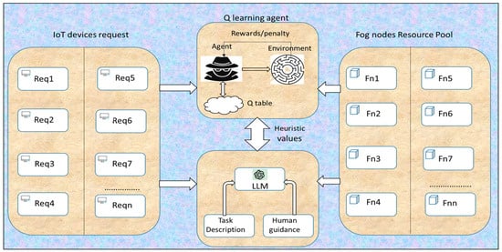
Figure 1. The high-level architecture of LLM-guided Q-learning framework for resource provisioning.

The detailed working of the LLM_QL framework is as follows. The state space of the Q-learning agent represents a set of all possible states that a Q-learning agent encounters in the environment. It is an important component of Q-learning agent as it learns to formulate the optimal action depending on the prevailing states. The state space indicates all possible combinations of configurations that the environment is composed of. Each state is used to provide a unique experience for the agent. The state typically represents the condition of the system, i.e., resource usage, task load, latency, and energy consumption. The fog nodes are made to learn best resource allocation policies by consequently interacting with the environment. The Q values are updated using the Bellman equation. The agent performs actions, which include allocation of resources, migration of tasks from fog node to the cloud, and queuing of the task for execution at later stages. A positive reward is provided for actions such as less processing delay, effective load balance, and lesser service level violations. Similarly, a negative reward is provided for actions such as higher processing delay, frequent load imbalance, and higher service level violations. Traditional Q-learning agents suffer from dimensionality problems and they cannot update the state action pairs for all possible combinations. However, the Q-learning agent enriched with the heuristic guidance of LLM helps in easy generalization and can operate efficiently in large and continuous state space environments.

The environment setup for the Q-learning agent involves the state space, action space, reward function, and transition dynamics. A pre-built environment is used for implementation using Application Programming Interfaces (APIs) like OpenAI Gym and unity machine learning agents. The Q-learning process inputs the IoT device requests and processes them using the Bellman equation to determine the optimal fog node for servicing.

Algorithm 1 provides the working of the LLM-guided Q-learning framework in detail. The IoT device requests are mapped onto the best fit fog nodes by considering the action value computed by the LLM-guided Q-learning agent. The heuristic value encourages the thinking ability of the agent in reaching the goal state. While navigating the Q-learning agent, the landmark positions are given highest heuristic values, which makes the traversal easier. It converges rapidly to appropriate promising solutions instead of searching for the perfect solution. By performing limited sampling and putting constraints over the responses, LLMs are made capable enough to perform zero-shot learning in varying computing scenarios of the fog environment. The actor–critic Q-learning algorithm usually finds it difficult to derive the policies through the implicit exploration process. Just by applying sample efficiency, proper reward reshaping is not possible and often ends up with the wrong heuristic value. Hence, the use of LLMs represents a promising approach for reward reshaping through autonomous state space exploration for Q-learning agents. Any possible inaccuracies in the learning steps are handled through fine tuning of the learning steps, which enhances the speed of inference and minimizes the impact of hallucination.

Algorithm 1: Working of LLM-guided Q-learning framework

1: Start 2: Input: IoT device request set: $\mathit{I}\mathit{o}\mathit{T}\left(\mathit{R}\mathit{E}\mathit{Q}\right)=\{{\mathit{R}\mathit{e}\mathit{q}}_1,{\mathit{R}\mathit{e}\mathit{q}}_2,{\mathit{R}\mathit{e}\mathit{q}}_3,{\mathit{R}\mathit{e}\mathit{q}}_4,\dots ,{\mathit{R}\mathit{e}\mathit{q}}_{\mathit{n}}\}$, Markov Decision Process MDP, Large Language Model G, Prompt P 3: Output: Resource provisioning policies i.e., R$\mathit{P}\mathit{P}=\{{\mathit{R}\mathit{p}\mathit{p}}_1,{\mathit{R}\mathit{p}\mathit{p}}_2,{\mathit{R}\mathit{p}\mathit{p}}_3,{\mathit{R}\mathit{p}\mathit{p}}_4,\dots ,{\mathit{R}\mathit{p}\mathit{p}}_{\mathit{n}}\}$ 4: Training phase of LLM_QL 5:    Initialize the Heuristic Q buffer: MDP(G(P)), actor-critic $\left({\mathit{\mu }}_{\mathbf{\varnothing }},{\mathit{Q}}_{\mathit{\theta }1},{\mathit{Q}}_{\mathit{\theta }2}\right)=\mathit{N}\mathit{U}\mathit{L}\mathit{L}$, and target actor-critic $\left({\mathit{\mu }}_{{\mathbf{\varnothing }}^{\prime }},{\mathit{Q}}_{{\mathit{\theta }1}^{\prime }},{\mathit{Q}}_{{\mathit{\theta }2}^{\prime }}\right)=\mathit{N}\mathit{U}\mathit{L}\mathit{L}$ 6:     Generate Q buffer: ${\mathit{D}}_{\mathit{g}}\leftarrow \left\{\right({\mathit{S}}_{\mathit{i}},{\mathit{a}}_{\mathit{i}},{\mathit{Q}}_{\mathit{i}}\left)\right|\left({\mathit{S}}_{\mathit{i}},{\mathit{a}}_{\mathit{i}},{\mathit{Q}}_{\mathit{i}}\right)\in \mathit{M}\mathit{D}\mathit{P}\left(\mathit{G}\left(\mathit{P}\right)\right),\mathit{i}=\mathrm{1,2},\dots ,\mathit{n}\}$, where ${\mathit{S}}_{\mathit{i}}$ = state of the agent at time step i, ${\mathit{a}}_{\mathit{i}}=$ action performed at time step i, and ${\mathit{Q}}_{\mathit{i}}=$ Q value for action ${\mathit{a}}_{\mathit{i}}$ in state ${\mathit{S}}_{\mathit{i}}$. 7:    Q Bootstrapping $\mathit{\theta }=\mathit{\theta }-\mathit{\alpha }{\nabla }_{\mathit{\theta }}{\mathit{L}}_{\mathit{B}\mathit{o}\mathit{o}\mathit{t}\mathit{s}\mathit{t}\mathit{r}\mathit{a}\mathit{p}}$ 8:       ${\mathit{L}}_{\mathit{B}\mathit{o}\mathit{o}\mathit{t}\mathit{s}\mathit{t}\mathit{r}\mathit{a}\mathit{p}}\left(\mathit{\theta }\right)={\mathit{E}}_{\left({\mathit{S}}_{\mathit{i}},{\mathit{a}}_{\mathit{i}},{\mathit{Q}}_{\mathit{i}}\right)\approx {\mathit{D}}_{\mathit{g}}}{({\mathit{Q}}_{\mathit{i}}-{\mathit{q}}_{\mathit{\theta }}^{\mathsf{\Lambda }}\left({\mathit{S}}_{\mathit{i}},{\mathit{a}}_{\mathit{i}}\right))}^2$ 9:   For each IoT device request in request task set ${\mathit{R}\mathit{e}\mathit{q}}_{\mathit{i}}\in \mathit{I}\mathit{o}\mathit{T}\left(\mathit{R}\mathit{E}\mathit{Q}\right)$ do 10:    Perform sampling of the Q state $\left({\mathit{S}}_{\mathit{i}},{\mathit{a}}_{\mathit{i}},{\mathit{r}}_{\mathit{i}},{\mathit{S}}_{\mathit{i}}^{\prime }\right)$ from the fog state space, ${\mathit{r}}_{\mathit{i}}$ = reward received for the action ${\mathit{a}}_{\mathit{i}}$ 11:     Compute Q buffer ${\mathit{D}}_{\mathit{g}}={\mathit{D}}_{\mathit{g}}\cup \left({\mathit{S}}_{\mathit{i}},{\mathit{a}}_{\mathit{i}},{\mathit{r}}_{\mathit{i}},{\mathit{S}}^{\prime }\right)$ 12:    Perform sampling over the computed value of the Q buffer ${\mathit{D}}_{\mathit{g}}$ 13:    ${\mathit{\alpha }}^{^}=\mathit{\mu }\left({\mathit{S}}_{\mathit{i}}^{\prime }\right)+\in ,$ where $\in =\mathit{c}\mathit{l}\mathit{i}\mathit{p}(\mathbb{N}\left(0,\mathit{\sigma }\right),-\mathit{c},\mathit{c})$ 14:    $\mathit{y}\left({\mathit{S}}_{\mathit{i}}^{\prime }\right)=(\mathit{r}+\mathit{\gamma }\mathbf{m}\mathbf{i}\mathbf{n}({\mathit{q}}_{\mathit{\theta }}({\mathit{S}}_{\mathit{i}}^{\prime },{\mathit{a}}^{^}$)) 15:    Update the critic ${\mathit{\theta }}_{\mathit{i}}={\mathit{a}\mathit{r}\mathit{g}\mathit{m}\mathit{i}\mathit{n}}_{{\mathit{\theta }}_{\mathit{i}}}\times {\mathit{L}}_{\mathit{m}\mathit{a}\mathit{j}\mathit{o}\mathit{r}}\left({\mathit{\theta }}_{\mathit{i}}\right)$ 16:    if t mod ${\mathit{D}}_{\mathit{g}}$ == 0 then 17:     Update actor $\mathbf{\varnothing }={\mathit{a}\mathit{r}\mathit{g}\mathit{m}\mathit{i}\mathit{n}}_{\mathbf{\varnothing }}\mathbf{*}{\mathit{L}}_{\mathit{a}\mathit{c}\mathit{t}\mathit{o}\mathit{r}}\left(\mathbf{\varnothing }\right)$ 18:     Update the target networks 19:       ${\mathit{\theta }}_{\mathit{i}}^{\prime }=\mathit{\tau }{\mathit{\theta }}_{\mathit{i}}+(1-\mathit{\tau }){\mathit{\theta }}_{\mathit{i}}^{\prime }$ 20:       $\mathit{\varnothing }=\mathit{\tau }\mathit{\varnothing }+(1-\mathit{\tau })\mathit{\varnothing }$ 21:      End if 22:   End for 23: End Training phase of LLM_QL 24: Testing phase of LLM_QL 25:     For each testing iteration t of IoT device request in request task set ${\mathit{R}\mathit{e}\mathit{q}}_{\mathit{i}}\in \mathit{I}\mathit{o}\mathit{T}\left(\mathit{R}\mathit{E}\mathit{Q}\right)$ do 26:    Re-compute Q buffer ${\mathit{D}}_{\mathit{g}}^{\prime }={\mathit{D}}_{\mathit{g}}^{\prime }\cup \left({\mathit{S}}_{\mathit{i}},{\mathit{a}}_{\mathit{i}},{\mathit{r}}_{\mathit{i}},{\mathit{S}}^{\prime }\right)$, where ${\mathit{D}}_{\mathit{g}}^{\prime }$ represent the memory buffer 27:    Compute the updated value of the critic ${\mathit{\theta }}_{\mathit{i}}^{″}={\mathit{a}\mathit{r}\mathit{g}\mathit{m}\mathit{i}\mathit{n}}_{{\mathit{\theta }}_{\mathit{i}}}\mathbf{\ast }{\mathit{L}}_{\mathit{m}\mathit{a}\mathit{j}\mathit{o}\mathit{r}}\left({\mathit{\theta }}_{\mathit{i}}\right)$ 28:    Update the critic ${\mathit{\theta }}_{\mathit{i}}^{″}={\mathit{a}\mathit{r}\mathit{g}\mathit{m}\mathit{i}\mathit{n}}_{{\mathit{\theta }}_{\mathit{i}}}\mathbf{\ast }{\mathit{L}}_{\mathit{m}\mathit{a}\mathit{j}\mathit{o}\mathit{r}}\left({\mathit{\theta }}_{\mathit{i}}\right)$ 29:    Update the target networks 30:       ${\mathit{\theta }}_{\mathit{i}}^{″}=\mathit{\tau }{\mathit{\theta }}_{\mathit{i}}^{\prime }+(1-\mathit{\tau }){\mathit{\theta }}_{\mathit{i}}^{″}$ 31:       ${\mathit{\varnothing }}^{\prime }=\mathit{\tau }{\mathit{\varnothing }}^{\prime }+(1-\mathit{\tau }){\mathit{\varnothing }}^{\prime }$ 32:    End For 33: End Testing phase of LLM_QL 34: Output $\mathit{R}\mathit{P}\mathit{P}=\{{\mathit{R}\mathit{p}\mathit{p}}_1,{\mathit{R}\mathit{p}\mathit{p}}_2,{\mathit{R}\mathit{p}\mathit{p}}_3,{\mathit{R}\mathit{p}\mathit{p}}_4,\dots ,{\mathit{R}\mathit{p}\mathit{p}}_{\mathit{n}}\}$ 35: Stop

5. Expected Value Analysis

The expected value analysis of the proposed LLM_QL is performed by considering four objective functions, i.e., processing delay, energy consumption, load imbalance, and service level agreement violation. Two types of fog computing scenarios are considered for analysis purposes, i.e., finite fog computing scenarios and infinite fog computing scenarios. The four objective functions (OFs) considered for analysis purpose are Processing Delay (PD(LLM_QL)), Energy Consumption (EC(LLM_QL)), Load (LD(LLM_QL)), and Service Level Agreement Violation (SLAV(LLM_QL)). The performance of the proposed LLM_QL is compared with three of the recent existing works, i.e., Bayesian Learning (BAY_L) [12], Centralized Controller (CC) [14], and Fuzzy Q Learning (F_QL) [15].

5.1. Finite Fog Computing Scenario

The finite fog computing scenario consists of N number of IoT device requests $REQ=\{{Req}_1, {Req}_2,{Req}_3,\dots ,{Req}_n\}$, K fog computing nodes $FN=\{{fn}_1, {fn}_2,{fn}_3,\dots ,{fn}_n\}$, and P resource provisioning policies $\pi =<{\pi }_1, {\pi }_2,{\pi }_3,\dots ,{\pi }_p>$. The probability of the outcome of the objective functions varies between low, medium, or high $P\left(OF\right)=<Low,Medium,High>$.

OF1: Processing Delay (PD(LLM_QL)): The expected value of the processing delay of the proposed LLM_QL, i.e., EV(PD(LLM_QL)) is influenced by the expected value of the processing rate of the requests $EV\left(PR\left({Req}_i\right)\right)$ and the expected value of the size of the requests $EV\left(S\left({Req}_i\right)\right)$.

$$EV\left({\displaystyle \frac{PD\left(LLM\_QL\right)}{\pi }}, ∆T\right)={\int }_x^y{\displaystyle \frac{\sum _{aϵ\pi }PD\left(LLM\_QL\right)\left(a\right)}{\left|\pi \right|}}$$

$$EV\left({\displaystyle \frac{PD\left(LLM\_QL\right)}{\pi }}, ∆T\right)=\sum _{d\in D}d{\int }_x^y{\displaystyle \frac{\sum _{aϵ\pi }PD\left(LLM\_QL\right)\left(a\right)}{\left|\mathsf{\pi }\right|}}$$

$$\begin{gathered} EV\left({\displaystyle \frac{PD\left(LLM\_QL\right)}{\mathsf{\pi }}}, ∆T\right)={\displaystyle \frac{EV\left(1\times \pi \times {\sum }_{i=1}^{i=I}\frac{1}{PR\left({Req}_i\right)}\times S\left({Req}_i\right)\right)}{\pi }} \\ =\sum _{d\in D}d{\int }_q^Q\left[{\displaystyle \frac{1}{PR\left({Req}_i\right)}} \right]\times S\left({Req}_i\right)] \\ ={\int }_q^{Q}Q\times dP{\displaystyle \frac{\left[ \frac{1}{PR\left({Req}_i\right)}\right]\times S\left({Req}_i\right)]}{\pi }} \end{gathered}$$

PD(LLM_QL): $\mathit{E}\mathit{V}\left({\displaystyle \frac{\mathit{P}\mathit{D}(\mathit{L}\mathit{L}\mathit{M}\_\mathit{Q}\mathit{L})}{\mathsf{\Pi }}},\mathit{T}\right)\cong \mathit{l}\mathit{o}\mathit{w}$

$$EV\left({\displaystyle \frac{PD\left(BAY\_L\right)}{\pi }}, ∆T\right)={\int }_x^y{\displaystyle \frac{\sum _{aϵ\pi }PD\left(BAY\_L\right)\left(a\right)}{\left|\pi \right|}}$$

$$EV\left({\displaystyle \frac{PD\left(BAY\_L\right)}{\pi }}, ∆T\right)=\sum _{d\in D}d{\int }_x^y{\displaystyle \frac{\sum _{aϵ\pi }PD\left(BAY\_L\right)\left(a\right)}{\left|\mathsf{\pi }\right|}}$$

$$EV\left({\displaystyle \frac{PD\left(LLM\_QL\right)}{\mathsf{\pi }}}, ∆T\right)={\displaystyle \frac{EV\left(1\times \pi \times {\sum }_{i=1}^{i=I}\frac{P\left(data|\theta \right)\times P\left(\theta \right)}{P\left(data\right)}\right)}{\pi }}$$

PD(BAY_L) = $\mathit{E}\mathit{V}\left({\displaystyle \frac{\mathit{P}\mathit{D}\left(\mathit{B}\mathit{A}\mathit{Y}\_\mathit{L}\right)}{\mathsf{\Pi }}},\mathit{T}\right)\cong \mathit{H}\mathit{i}\mathit{g}\mathit{h}$

$$EV\left({\displaystyle \frac{PD\left(CC\right)}{\pi }}, ∆T\right)={\int }_x^y{\displaystyle \frac{\sum _{aϵ\pi }PD\left(CC\right)\left(a\right)}{\left|\pi \right|}}$$

$$EV\left({\displaystyle \frac{PD\left(CC\right)}{\pi }}, ∆T\right)=\sum _{d\in D}d{\int }_x^y{\displaystyle \frac{\sum _{aϵ\pi }PD\left(CC\right)\left(a\right)}{\left|\mathsf{\pi }\right|}}$$

$$EV\left({\displaystyle \frac{PD\left(CC\right)}{\mathsf{\pi }}}, ∆T\right)={\displaystyle \frac{EV\left(1\times \pi \times {\sum }_{i=1}^{i=I}f(x\left(t\right),r\left(t\right),P)\right)}{\pi }}$$

where f(x(t),r(t),P) = System state, Desired setpoint, and system parameters.

PD(CC) = $\mathit{E}\mathit{V}\left({\displaystyle \frac{\mathit{P}\mathit{D}\left(\mathit{C}\mathit{C}\right)}{\mathsf{\Pi }}},\mathit{T}\right)\cong \mathit{M}\mathit{e}\mathit{d}\mathit{i}\mathit{u}\mathit{m}$

$$EV\left({\displaystyle \frac{PD\left(F\_QL\right)}{\pi }}, ∆T\right)={\int }_x^y{\displaystyle \frac{\sum _{aϵ\pi }PD\left(F\_QL\right)\left(a\right)}{\left|\pi \right|}}$$

$$EV\left({\displaystyle \frac{PD\left(F\_QL\right)}{\pi }}, ∆T\right)=\sum _{d\in D}d{\int }_x^y{\displaystyle \frac{\sum _{aϵ\pi }PD\left(F\_QL\right)\left(a\right)}{\left|\mathsf{\pi }\right|}}$$

$$EV\left({\displaystyle \frac{PD\left(F\_QL\right)}{\mathsf{\pi }}}, ∆T\right)={\displaystyle \frac{EV\left(1\ast \pi \ast Q\left(s,a\right)+\propto (R+\gamma \max Q^{\prime }\left(s,a\right)-Q(s,a)\right)}{\pi }}$$

PD(F_QL) = $\mathit{E}\mathit{V}\left({\displaystyle \frac{\mathit{P}\mathit{D}\left(\mathit{F}\_\mathit{Q}\mathit{L}\right)}{\mathsf{\Pi }}},\mathit{T}\right)\cong \mathit{H}\mathit{i}\mathit{g}\mathit{h}$

OF2: Energy Consumption (EC(LLM_QL)): The expected value of the energy consumption of the proposed LLM_QL, i.e., EV(EC(LLM_QL)) is influenced by the expected value of the power required to process the input requests $EV\left(PC\left({Req}_i\right)\right)$, workload allocated $EV\left(WL\left({Req}_i\right)\right)$, and computational capacity of the fog node $EV\left(CP\left({fn}_i\right)\right)$.

$$EV\left({\displaystyle \frac{EC\left(LLM\_QL\right)}{\mathsf{\pi }}}, ∆T\right)={\int }_x^y{\displaystyle \frac{\sum _{aϵ\pi }EC\left(LLM\_QL\right)\left(a\right)}{\left|\pi \right|}}$$

$$EV\left({\displaystyle \frac{EC\left(LLM\_QL\right)}{\mathsf{\pi }}}, ∆T\right)=\sum _{d\in D}d{\int }_x^y{\displaystyle \frac{\sum _{aϵ\pi }EC\left(LLM\_QL\right)\left(a\right)}{\left|\mathsf{\pi }\right|}}$$

$$\begin{gathered} EV\left({\displaystyle \frac{EC\left(LLM\_QL\right)}{\pi }}, ∆T\right)={\displaystyle \frac{E\left(1\times \pi \times {\sum }_{i=1}^{i=I}PC\left({Req}_i\right)\times \frac{WL\left({Req}_i\right)}{CP(\left({fn}_i\right)}\right)}{P\left(\mathsf{\pi }\right)}} \\ =\sum _{d\in D}d{\int }_q^Q[PC\left({Req}_i\right)\times {\displaystyle \frac{WL\left({Req}_i\right)}{CP(\left({fn}_i\right)}}] \\ ={\int }_q^{Q}Q\times dP{\displaystyle \frac{\left[ PC\left({Req}_i\right)\right]\times \frac{WL\left({Req}_i\right)}{CP(\left({fn}_i\right)}]}{\mathsf{\pi }}} \end{gathered}$$

EC(LLM_QL): $\mathit{E}\mathit{V}\left({\displaystyle \frac{\mathit{E}\mathit{C}(\mathit{L}\mathit{L}\mathit{M}\_\mathit{Q}\mathit{L})}{\mathsf{\Pi }}},\mathit{T}\right)\cong \mathit{L}\mathit{o}\mathit{w}$

$$EV\left({\displaystyle \frac{EC\left(BAY\_L\right)}{\mathsf{\pi }}}, ∆T\right)={\int }_x^y{\displaystyle \frac{\sum _{aϵ\pi }EC\left(LLM\_QL\right)\left(a\right)}{\left|\pi \right|}}$$

$$E\left({\displaystyle \frac{EC\left(BAy\_L\right)}{\mathsf{\pi }}}, ∆T\right)=\sum _{d\in D}d{\int }_x^y{\displaystyle \frac{\sum _{aϵ\pi }EC\left(LLM\_QL\right)\left(a\right)}{\left|\mathsf{\pi }\right|}}$$

$$E\left({\displaystyle \frac{EC\left(BAY\_L\right)}{\pi }}, ∆T\right)={\displaystyle \frac{E\left(1\times \pi \times {\sum }_{i=1}^{i=I}PC\left({Req}_i\right)\times \frac{P\left(data|\theta \right)\times P\left(\theta \right)}{P\left(data\right)}\right)}{P\left(\mathsf{\pi }\right)}}$$

EC(BAY_L) = $\mathit{E}\mathit{V}\left({\displaystyle \frac{\mathit{E}\mathit{C}\left(\mathit{B}\mathit{A}\mathit{Y}\_\mathit{L}\right)}{\mathsf{\Pi }}},\mathit{T}\right)\cong \mathit{M}\mathit{e}\mathit{d}\mathit{i}\mathit{u}\mathit{m}$

$$EV\left({\displaystyle \frac{EC\left(CC\right)}{\mathsf{\pi }}}, ∆T\right)={\int }_x^y{\displaystyle \frac{\sum _{aϵ\pi }EC\left(LLM\_QL\right)\left(a\right)}{\left|\pi \right|}}$$

$$E\left({\displaystyle \frac{EC\left(CC\right)}{\mathsf{\pi }}}, ∆T\right)=\sum _{d\in D}d{\int }_x^y{\displaystyle \frac{\sum _{aϵ\pi }EC\left(LLM\_QL\right)\left(a\right)}{\left|\mathsf{\pi }\right|}}$$

$$E\left({\displaystyle \frac{EC\left(CC\right)}{\pi }}, ∆T\right)={\displaystyle \frac{E\left(1\times \pi {\sum }_{i=1}^{i=I}PC\left({Req}_i\right)\times f(x\left(t\right),r\left(t\right),P)\right)}{P\left(\mathsf{\pi }\right)}}$$

EC(CC) = $\mathit{E}\mathit{V}\left({\displaystyle \frac{\mathit{E}\mathit{C}\left(\mathit{C}\mathit{C}\right)}{\mathsf{\Pi }}},\mathit{T}\right)\cong \mathit{H}\mathit{i}\mathit{g}\mathit{h}$

$$EV\left({\displaystyle \frac{EC\left(F\_QL\right)}{\mathsf{\pi }}}, ∆T\right)={\int }_x^y{\displaystyle \frac{\sum _{aϵ\pi }EC\left(F\_QL\right)\left(a\right)}{\left|\pi \right|}}$$

$$EV\left({\displaystyle \frac{EC\left(F\_QL\right)}{\mathsf{\pi }}}, ∆T\right)=\sum _{d\in D}d{\int }_x^y{\displaystyle \frac{\sum _{aϵ\pi }EC\left(F\_QL\right)\left(a\right)}{\left|\mathsf{\pi }\right|}}$$

$$EV\left({\displaystyle \frac{EC\left(F\_QL\right)}{\pi }}, ∆T\right)={\displaystyle \frac{EV\left(1\times \pi \times {\sum }_{i=1}^{i=I}PC\left({Req}_i\right)\times Q\left(s,a\right)+\propto (R+\gamma \max Q^{\prime }\left(s,a\right)-Q(s,a))\right)}{P\left(\mathsf{\pi }\right)}}$$

EC(F_QL) =$\mathit{E}\mathit{V}\left({\displaystyle \frac{\mathit{E}\mathit{C}\left(\mathit{F}\_\mathit{Q}\mathit{L}\right)}{\mathsf{\Pi }}},\mathit{T}\right)\cong \mathit{M}\mathit{e}\mathit{d}\mathit{i}\mathit{u}\mathit{m}$

OF3: Load (LD(LLM_QL)): The expected value of the load on the proposed LLM_QL, i.e., EV(LD(LLM_QL)) is influenced by the expected value of the request processing time $EV\left(PT\right({Req}_i$)) and number of requests generated $EV\left(N\left({Req}_i,∆T\right)\right).$

$$EV\left({\displaystyle \frac{LD\left(LLM\_QL\right)}{\pi }}, ∆T\right)={\int }_x^y{\displaystyle \frac{\sum _{aϵ\pi }LD\left(LLM\_QL\right)\left(a\right)}{\left|\pi \right|}}$$

$$EV\left({\displaystyle \frac{LD\left(LLM\_QL\right)}{\pi }}, ∆T\right)=\sum _{d\in D}d{\int }_x^y{\displaystyle \frac{\sum _{aϵ\pi }LD\left(LLM\_QL\right)\left(a\right)}{\left|\mathsf{\pi }\right|}}$$

$$\begin{gathered} EV\left({\displaystyle \frac{LD(LLM\_QL)}{\pi }}, ∆T\right)={\displaystyle \frac{EV\left(1\times \pi \times {\sum }_{i=1}^{i=I}\frac{Mean\left({N(fn}_i)\right)\times N\left({Req}_i\right)}{N\left({fn}_i\right)\times CC\left({fn}_i\right)}\right)}{P\left(\mathsf{\pi }\right)}} \\ =\sum _{d\in D}d{\int }_q^Q{\displaystyle \frac{Mean\left({N(fn}_i)\right)\times N\left({Req}_i\right)}{N\left({fn}_i\right)\times CC\left({fn}_i\right)}} \\ ={\int }_q^{Q}Q\times dP{\displaystyle \frac{\frac{Mean\left({N(fn}_i)\right)\times N\left({Req}_i\right)}{N\left({fn}_i\right)\times CC\left({fn}_i\right)}}{\pi }} \end{gathered}$$

LD(LLM_QL): $\mathit{E}\mathit{V}\left({\displaystyle \frac{\mathit{L}\mathit{D}(\mathit{L}\mathit{L}\mathit{M}\_\mathit{Q}\mathit{L})}{\mathsf{\Pi }}},\mathit{T}\right)\cong \mathit{B}\mathit{a}\mathit{l}\mathit{a}\mathit{n}\mathit{c}\mathit{e}\mathit{d}$

$$EV\left({\displaystyle \frac{LD\left(BAY\_L\right)}{\pi }}, ∆T\right)={\int }_x^y{\displaystyle \frac{\sum _{aϵ\pi }LD\left(BAY\_L\right)\left(a\right)}{\left|\pi \right|}}$$

$$EV\left({\displaystyle \frac{LD\left(BAY\_L\right)}{\pi }}, ∆T\right)=\sum _{d\in D}d{\int }_x^y{\displaystyle \frac{\sum _{aϵ\pi }LD\left(BAY\_L\right)\left(a\right)}{\left|\mathsf{\pi }\right|}}$$

$$EV\left({\displaystyle \frac{LD(BAY\_L)}{\pi }}, ∆T\right)={\displaystyle \frac{EV\left(1\times \pi \times {\sum }_{i=1}^{i=I}\frac{Mean\_Load}{Peak\_Load}\right)}{P\left(\mathsf{\pi }\right)}}$$

LD(BAY_L) = $\mathit{E}\mathit{V}\left({\displaystyle \frac{\mathit{L}\mathit{D}\left(\mathit{B}\mathit{A}\mathit{Y}\_\mathit{L}\right)}{\mathsf{\Pi }}},\mathit{T}\right)\cong \mathit{P}\mathit{a}\mathit{r}\mathit{t}\mathit{i}\mathit{a}\mathit{l}\mathit{l}\mathit{y} \mathit{B}\mathit{a}\mathit{l}\mathit{a}\mathit{n}\mathit{c}\mathit{e}\mathit{d}$

$$EV\left({\displaystyle \frac{LD\left(CC\right)}{\pi }}, ∆T\right)={\int }_x^y{\displaystyle \frac{\sum _{aϵ\pi }LD\left(CC\right)\left(a\right)}{\left|\pi \right|}}$$

$$EV\left({\displaystyle \frac{LD\left(CC\right)}{\pi }}, ∆T\right)=\sum _{d\in D}d{\int }_x^y{\displaystyle \frac{\sum _{aϵ\pi }LD\left(CC\right)\left(a\right)}{\left|\mathsf{\pi }\right|}}$$

$$EV\left({\displaystyle \frac{LD\left(CC\right)}{\pi }}, ∆T\right)={\displaystyle \frac{EV\left(1\times \pi \times {\sum }_{i=1}^{i=I}\frac{CP\left({fn}_i\right)}{Load\left({fn}_i\right)}\times f(x\left(t\right),r\left(t\right),P)\right)}{P\left(\mathsf{\pi }\right)}}$$

LD(CC) = $\mathit{E}\mathit{V}\left({\displaystyle \frac{\mathit{L}\mathit{D}\left(\mathit{C}\mathit{C}\right)}{\mathsf{\Pi }}},\mathit{T}\right)\cong \mathit{I}\mathit{m}\mathit{b}\mathit{a}\mathit{l}\mathit{a}\mathit{n}\mathit{c}\mathit{e}\mathit{d}$

$$EV\left({\displaystyle \frac{LD\left(F\_QL\right)}{\pi }}, ∆T\right)={\int }_x^y{\displaystyle \frac{\sum _{aϵ\pi }LD\left(F\_QL\right)\left(a\right)}{\left|\pi \right|}}$$

$$EV\left({\displaystyle \frac{LD\left(F\_QL\right)}{\pi }}, ∆T\right)=\sum _{d\in D}d{\int }_x^y{\displaystyle \frac{\sum _{aϵ\pi }LD\left(F\_QL\right)\left(a\right)}{\left|\mathsf{\pi }\right|}}$$

$$\begin{array}{ll}EV\left({\displaystyle \frac{LD(F\_QL)}{\pi }}, ∆T\right)& \\ & ={\displaystyle \frac{EV\left(1\times \pi \times {\sum }_{i=1}^{i=I}\frac{CP\left({Req}_i\right)}{Load\left({Req}_i\right)}\times Q\left(s,a\right)+\propto (R+\gamma \max Q^{\prime }\left(s,a\right)-Q\left(s,a\right))\right)}{P\left(\mathsf{\pi }\right)}}\end{array}$$

LD(F_QL) =$\mathit{E}\mathit{V}\left({\displaystyle \frac{\mathit{L}\mathit{D}\left(\mathit{F}\_\mathit{Q}\mathit{L}\right)}{\mathsf{\Pi }}},\mathit{T}\right)\cong \mathit{I}\mathit{m}\mathit{b}\mathit{a}\mathit{l}\mathit{a}\mathit{n}\mathit{c}\mathit{e}\mathit{d}$

OF4: Service Level Agreement Violation (SLAV(LLM_QL)): The expected value of the Service Level Agreement Violation of the proposed LLM_QL, i.e., EV(SLAV(LLM_QL)) is influenced by the expected value of the request processing time $EV\left(PT\right({Req}_i$)).

$$EV\left({\displaystyle \frac{SLAV\left(LLM\_QL\right)}{\mathsf{\pi }}}, ∆T\right)={\int }_x^y{\displaystyle \frac{\sum _{aϵ\pi }SLAV\left(LLM\_QL\right)\left(a\right)}{\left|\pi \right|}}$$

$$EV\left({\displaystyle \frac{SLAV\left(LLM\_QL\right)}{\mathsf{\pi }}}, ∆T\right)=\sum _{d\in D}d{\int }_x^y{\displaystyle \frac{\sum _{aϵ\pi }SLAV\left(LLM\_QL\right)\left(a\right)}{\left|\mathsf{\pi }\right|}}$$

$$\begin{gathered} E\left({\displaystyle \frac{SLAV\left(LLM\_QL\right)}{\pi }}, ∆T\right)={\displaystyle \frac{E\left(1\times \pi \times {\sum }_{i=1}^{i=n}PT\left({Req}_i,∆T\right)\right)}{P\left(\mathsf{\pi }\right)}} \\ =\sum _{d\in D}d{\int }_q^{Q}Minimize\left\{\begin{array}{c}SLAV=Yes, if PT\left({Req}_i,∆T\right)>0\\ SLAV=No, if PT\left({Req}_i,∆T\right)\le 0\end{array}\right. \\ ={\int }_q^{Q}Q\times dP{\displaystyle \frac{\left[ SLAV=No, \forall PT\left({Req}_i,∆T\right)\le 0\right]]}{\mathsf{\pi }}} \end{gathered}$$

SLAV(LLM_QL): $\mathit{E}\mathit{V}\left({\displaystyle \frac{\mathit{S}\mathit{L}\mathit{A}\mathit{V}(\mathit{L}\mathit{L}\mathit{M}\_\mathit{Q}\mathit{L})}{\mathsf{\Pi }}},\mathit{T}\right)\cong \mathit{L}\mathit{o}\mathit{w}$

$$EV\left({\displaystyle \frac{SLAV\left(BAY\_L\right)}{\mathsf{\pi }}}, ∆T\right)={\int }_x^y{\displaystyle \frac{\sum _{aϵ\pi }SLAV\left(BAY\_L\right)\left(a\right)}{\left|\pi \right|}}$$

$$EV\left({\displaystyle \frac{SLAV\left(BAY\_L\right)}{\mathsf{\pi }}}, ∆T\right)=\sum _{d\in D}d{\int }_x^y{\displaystyle \frac{\sum _{aϵ\pi }SLAV\left(BAY\_L\right)\left(a\right)}{\left|\mathsf{\pi }\right|}}$$

$$E\left({\displaystyle \frac{SLAV\left(BAY\_L\right)}{\pi }}, ∆T\right)=\sum _{d\in D}d{\int }_q^Q\mathrm{S}LAV=Yes, \forall PT\left({Req}_i,∆T\right)\ge 0$$

SLAV(BAY_L) = $\mathit{E}\mathit{V}\left({\displaystyle \frac{\mathit{S}\mathit{L}\mathit{A}\mathit{V}\left(\mathit{B}\mathit{A}\mathit{Y}\_\mathit{L}\right)}{\mathsf{\Pi }}},\mathit{T}\right)\cong \mathit{M}\mathit{e}\mathit{d}\mathit{i}\mathit{u}\mathit{m}$

$$EV\left({\displaystyle \frac{SLAV\left(CC\right)}{\mathsf{\pi }}}, ∆T\right)={\int }_x^y{\displaystyle \frac{\sum _{aϵ\pi }SLAV\left(CC\right)\left(a\right)}{\left|\pi \right|}}$$

$$EV\left({\displaystyle \frac{SLAV\left(CC\right)}{\mathsf{\pi }}}, ∆T\right)=\sum _{d\in D}d{\int }_x^y{\displaystyle \frac{\sum _{aϵ\pi }SLAV\left(CC\right)\left(a\right)}{\left|\mathsf{\pi }\right|}}$$

$$E\left({\displaystyle \frac{SLAV\left(CC\right)}{\pi }}, ∆T\right)=\sum _{d\in D}d{\int }_q^Q\mathrm{S}LAV=Yes, \forall PT\left({Req}_i,∆T\right)\ge 0$$

SLAV(CC) = $\mathit{E}\mathit{V}\left({\displaystyle \frac{\mathit{S}\mathit{L}\mathit{A}\mathit{V}\left(\mathit{C}\mathit{C}\right)}{\mathsf{\Pi }}},\mathit{T}\right)\cong \mathit{H}\mathit{i}\mathit{g}\mathit{h}$

$$EV\left({\displaystyle \frac{SLAV\left(F\_QL\right)}{\mathsf{\pi }}}, ∆T\right)={\int }_x^y{\displaystyle \frac{\sum _{aϵ\pi }SLAV\left(F\_QL\right)\left(a\right)}{\left|\pi \right|}}$$

$$EV\left({\displaystyle \frac{SLAV\left(F\_QL\right)}{\mathsf{\pi }}}, ∆T\right)=\sum _{d\in D}d{\int }_x^y{\displaystyle \frac{\sum _{aϵ\pi }SLAV\left(F\_QL\right)\left(a\right)}{\left|\mathsf{\pi }\right|}}$$

$$E\left({\displaystyle \frac{SLAV\left(F\_QL\right)}{\pi }}, ∆T\right)=\sum _{d\in D}d{\int }_q^Q\mathrm{S}LAV=Yes, \forall PT\left({Req}_i,∆T\right)\ge 0$$

SLAV(F_QL) = $\mathit{E}\mathit{V}\left({\displaystyle \frac{\mathit{S}\mathit{L}\mathit{A}\mathit{V}\left(\mathit{F}\_\mathit{Q}\mathit{L}\right)}{\mathsf{\Pi }}},\mathit{T}\right)\cong \mathit{H}\mathit{i}\mathit{g}\mathit{h}$

5.2. Infinite Fog Computing Scenario

The infinite fog computing scenario consists of an infinite number of IoT device requests $REQ=\{{Req}_1, {Req}_2,{Req}_3,\dots ,{Req}_{\infty }\}$, K fog computing nodes $FN=\{{fn}_1, {fn}_2,{fn}_3,\dots ,{fn}_{\infty }\}$, and $\infty$ resource provisioning policies $\pi =<{\pi }_1, {\pi }_2,{\pi }_3,\dots ,{\pi }_{\infty }>$.

OF1: Processing Delay (PD(LLM_QL)): The EV(PD(LLM_QL)) during the infinite scenario remained less compared to EV(PD(LLM_QL)) during the finite scenario.

$$EV\left({\displaystyle \frac{PD\left(LLM\_QL\right)}{\pi }}, ∆T\right)={\int }_{-\infty }^0{\displaystyle \frac{\sum _{aϵ\pi }PD\left(LLM\_QL\right)\left(a\right)}{\left|\pi \right|}}+{\int }_0^{+\infty }{\displaystyle \frac{\sum _{aϵ\pi }PD\left(LLM\_QL\right)\left(a\right)}{\left|\pi \right|}}$$

$$EV\left({\displaystyle \frac{PD\left(LLM\_QL\right)}{\pi }}, ∆T\right)=\sum _{d\in D}d{\int }_{-\infty }^0{\displaystyle \frac{\sum _{aϵ\pi }PD\left(LLM\_QL\right)\left(a\right)}{\left|\mathsf{\pi }\right|}}+{\int }_0^{\infty }{\displaystyle \frac{\sum _{aϵ\pi }PD\left(LLM\_QL\right)\left(a\right)}{\left|\mathsf{\pi }\right|}}$$

$$\begin{gathered} EV\left({\displaystyle \frac{PD\left(LLM\_QL\right)}{\mathsf{\pi }}}, ∆T\right)={\int }_{-\infty }^{+\infty }{\displaystyle \frac{EV\left(1\times \pi \times {\sum }_{i=1}^{i=I}\frac{1}{PR\left({Req}_i\right)}\times S\left({Req}_i\right)\right)}{\pi }} \\ =\sum _{d\in D}d{\int }_{-\infty }^{+\infty }\left[{\displaystyle \frac{1}{PR\left({Req}_i\right)}} \right]\times S\left({Req}_i\right)] \\ ={\int }_{-\infty }^{+\infty }Q\times dP{\displaystyle \frac{\left[ \frac{1}{PR\left({Req}_i\right)}\right]\times S\left({Req}_i\right)]}{\pi }} \end{gathered}$$

PD(LLM_QL): $\mathit{E}\mathit{V}\left({\displaystyle \frac{\mathit{P}\mathit{D}(\mathit{L}\mathit{L}\mathit{M}\_\mathit{Q}\mathit{L})}{\mathsf{\Pi }}},\mathit{T}\right)\cong \mathit{l}\mathit{o}\mathit{w}$

$$EV\left({\displaystyle \frac{PD\left(BAY\_L\right)}{\pi }}, ∆T\right)={\int }_{-\infty }^0{\displaystyle \frac{\sum _{aϵ\pi }PD\left(BAY\_L\right)\left(a\right)}{\left|\pi \right|}}+{\int }_0^{+\infty }{\displaystyle \frac{\sum _{aϵ\pi }PD\left(BAY\_L\right)\left(a\right)}{\left|\pi \right|}}$$

$$EV\left({\displaystyle \frac{PD\left(BAY\_L\right)}{\pi }}, ∆T\right)=\sum _{d\in D}d{\int }_{-\infty }^0{\displaystyle \frac{\sum _{aϵ\pi }PD\left(BAY\_L\right)\left(a\right)}{\left|\mathsf{\pi }\right|}}+{\int }_0^{\infty }{\displaystyle \frac{\sum _{aϵ\pi }PD\left(BAY\_L\right)\left(a\right)}{\left|\mathsf{\pi }\right|}}$$

$$EV\left({\displaystyle \frac{PD\left(BAY\_L\right)}{\mathsf{\pi }}}, ∆T\right)={\int }_{-\infty }^{+\infty }{\displaystyle \frac{EV\left(1\times \pi \times {\sum }_{i=1}^{i=I}\frac{P\left(data|\theta \right)\ast P\left(\theta \right)}{P\left(data\right)}\right)}{\pi }}$$

PD(BAY_L) = $\mathit{E}\mathit{V}\left({\displaystyle \frac{\mathit{P}\mathit{D}\left(\mathit{B}\mathit{A}\mathit{Y}\_\mathit{L}\right)}{\mathsf{\Pi }}},\mathit{T}\right)\cong \mathit{H}\mathit{i}\mathit{g}\mathit{h}$

$$EV\left({\displaystyle \frac{PD\left(CC\right)}{\pi }}, ∆T\right)={\int }_{-\infty }^0{\displaystyle \frac{\sum _{aϵ\pi }PD\left(CC\right)\left(a\right)}{\left|\pi \right|}}+{\int }_0^{+\infty }{\displaystyle \frac{\sum _{aϵ\pi }PD\left(CC\right)\left(a\right)}{\left|\pi \right|}}$$

$$EV\left({\displaystyle \frac{PD\left(CC\right)}{\pi }}, ∆T\right)=\sum _{d\in D}d{\int }_{-\infty }^0{\displaystyle \frac{\sum _{aϵ\pi }PD\left(CC\right)\left(a\right)}{\left|\mathsf{\pi }\right|}}+{\int }_0^{\infty }{\displaystyle \frac{\sum _{aϵ\pi }PD\left(CC\right)\left(a\right)}{\left|\mathsf{\pi }\right|}}$$

$$EV\left({\displaystyle \frac{PD\left(LL{M}_{QL}\right)}{\mathsf{\pi }}}, ∆T\right)={\int }_{-\infty }^{+\infty }{\displaystyle \frac{EV\left(1\times \pi \times {\sum }_{i=1}^{i=I}f(x\left(t\right),r\left(t\right),P)\right)}{\pi }}$$

PD(CC) = $\mathit{E}\mathit{V}\left({\displaystyle \frac{\mathit{P}\mathit{D}\left(\mathit{C}\mathit{C}\right)}{\mathsf{\Pi }}},\mathit{T}\right)\cong \mathit{H}\mathit{i}\mathit{g}\mathit{h}$

$$EV\left({\displaystyle \frac{PD\left(F\_QL\right)}{\pi }}, ∆T\right)={\int }_{-\infty }^0{\displaystyle \frac{\sum _{aϵ\pi }PD\left(F\_QL\right)\left(a\right)}{\left|\pi \right|}}+{\int }_0^{+\infty }{\displaystyle \frac{\sum _{aϵ\pi }PD\left(F\_QL\right)\left(a\right)}{\left|\pi \right|}}$$

$$EV\left({\displaystyle \frac{PD\left(F\_QL\right)}{\pi }}, ∆T\right)=\sum _{d\in D}d{\int }_{-\infty }^0{\displaystyle \frac{\sum _{aϵ\pi }PD\left(F\_QL\right)\left(a\right)}{\left|\mathsf{\pi }\right|}}+{\int }_0^{\infty }{\displaystyle \frac{\sum _{aϵ\pi }PD\left(F\_QL\right)\left(a\right)}{\left|\mathsf{\pi }\right|}}$$

$$EV\left({\displaystyle \frac{PD\left(F\_QL\right)}{\mathsf{\pi }}}, ∆T\right)={\int }_{-\infty }^{+\infty }{\displaystyle \frac{EV\left(1\times \pi \times {\sum }_{i=1}^{i=I}Q\left(s,a\right)+\propto (R+\gamma \max Q^{\prime }\left(s,a\right)-Q(s,a)\right)}{\pi }}$$

PD(F_QL) = $\mathit{E}\mathit{V}\left({\displaystyle \frac{\mathit{P}\mathit{D}\left(\mathit{F}\_\mathit{Q}\mathit{L}\right)}{\mathsf{\Pi }}},\mathit{T}\right)\cong \mathit{H}\mathit{i}\mathit{g}\mathit{h}$

OF2: Energy Consumption (EC(LLM_QL)): The EV(EC(LLM_QL)) during the infinite scenario is found to be less compared to EV(EC(LLM_QL)) during the finite scenario.

$$EV\left({\displaystyle \frac{EC\left(LLM\_QL\right)}{\mathsf{\pi }}}, ∆T\right)={\int }_{-\infty }^0{\displaystyle \frac{\sum _{aϵ\pi }EC\left(LLM\_QL\right)\left(a\right)}{\left|\pi \right|}}+{\int }_0^{+\infty }{\displaystyle \frac{\sum _{aϵ\pi }EC\left(LLM\_QL\right)\left(a\right)}{\left|\pi \right|}}$$

$$E\left({\displaystyle \frac{EC\left(LLM\_QL\right)}{\mathsf{\pi }}}, ∆T\right)={\sum }_{d\in D}d{\int }_{-\infty }^0{\displaystyle \frac{\sum _{aϵ\pi }EC\left(LLM\_QL\right)\left(a\right)}{\left|\mathsf{\pi }\right|}}+{\int }_0^{+\infty }{\displaystyle \frac{\sum _{aϵ\pi }EC\left(LLM\_QL\right)\left(a\right)}{\left|\mathsf{\pi }\right|}}$$

$$\begin{gathered} E\left({\displaystyle \frac{EC\left(LLM\_QL\right)}{\pi }}, ∆T\right)={\int }_{-\infty }^{+\infty }{\displaystyle \frac{E\left(1\times \pi \times {\sum }_{i=1}^{i=I}PC\left({Req}_i\right)\times \frac{WL\left({Req}_i\right)}{CP\left({fn}_i\right)}\right)}{P\left(\mathsf{\pi }\right)}} \\ =\sum _{d\in D}d{\int }_{-\infty }^{+\infty }[PC\left({Req}_i\right)\times {\displaystyle \frac{WL\left({Req}_i\right)}{CP\left({fn}_i\right)}}] \\ ={\int }_{-\infty }^{+\infty }Q\times dP{\displaystyle \frac{\left[ PC\left({Req}_i\right)\right]\ast \frac{WL\left({Req}_i\right)}{CP\left({fn}_i\right)}]}{\mathsf{\pi }}} \end{gathered}$$

EC(LLM_QL): $\mathit{E}\mathit{V}\left({\displaystyle \frac{\mathit{E}\mathit{C}(\mathit{L}\mathit{L}\mathit{M}\_\mathit{Q}\mathit{L})}{\mathsf{\Pi }}},\mathit{T}\right)\cong \mathit{L}\mathit{o}\mathit{w}$

$$EV\left({\displaystyle \frac{EC\left(BAY\_L\right)}{\mathsf{\pi }}}, ∆T\right)={\int }_{-\infty }^0{\displaystyle \frac{\sum _{aϵ\pi }EC\left(BAY\_L\right)\left(a\right)}{\left|\pi \right|}}+{\int }_0^{+\infty }{\displaystyle \frac{\sum _{aϵ\pi }EC\left(BAY\_L\right)\left(a\right)}{\left|\pi \right|}}$$

$$E\left({\displaystyle \frac{EC\left(BAY\_L\right)}{\mathsf{\pi }}}, ∆T\right)={\sum }_{d\in D}d{\int }_{-\infty }^0{\displaystyle \frac{\sum _{aϵ\pi }EC\left(BAY\_L\right)\left(a\right)}{\left|\mathsf{\pi }\right|}}+{\int }_0^{+\infty }{\displaystyle \frac{\sum _{aϵ\pi }EC\left(BAY\_L\right)\left(a\right)}{\left|\mathsf{\pi }\right|}}$$

$$E\left({\displaystyle \frac{EC\left(BAY\_L\right)}{\pi }}, ∆T\right)={\int }_{-\infty }^{+\infty }{\displaystyle \frac{E\left(1\times \pi \times \frac{P\left(data|\theta \right)\times P\left(\theta \right)}{P\left(data\right)}\right)}{P\left(\mathsf{\pi }\right)}}$$

EC(BAY_L) = $\mathit{E}\mathit{V}\left({\displaystyle \frac{\mathit{E}\mathit{C}\left(\mathit{E}\mathit{X}\mathit{W}1\right)}{\mathsf{\Pi }}},\mathit{T}\right)\cong \mathit{M}\mathit{e}\mathit{d}\mathit{i}\mathit{u}\mathit{m}$

$$EV\left({\displaystyle \frac{EC\left(CC\right)}{\mathsf{\pi }}}, ∆T\right)={\int }_{-\infty }^0{\displaystyle \frac{\sum _{aϵ\pi }EC\left(CC\right)\left(a\right)}{\left|\pi \right|}}+{\int }_0^{+\infty }{\displaystyle \frac{\sum _{aϵ\pi }EC\left(CC\right)\left(a\right)}{\left|\pi \right|}}$$

$$E\left({\displaystyle \frac{EC\left(CC\right)}{\mathsf{\pi }}}, ∆T\right)={\sum }_{d\in D}d{\int }_{-\infty }^0{\displaystyle \frac{\sum _{aϵ\pi }EC\left(CC\right)\left(a\right)}{\left|\mathsf{\pi }\right|}}+{\int }_0^{+\infty }{\displaystyle \frac{\sum _{aϵ\pi }EC\left(CC\right)\left(a\right)}{\left|\mathsf{\pi }\right|}}$$

$$E\left({\displaystyle \frac{EC\left(CC\right)}{\pi }}, ∆T\right)={\int }_{-\infty }^{+\infty }{\displaystyle \frac{E\left(1\times \pi \times {\sum }_{i=1}^{i=I}PC\left({Req}_i\right)\times f(x\left(t\right),r\left(t\right),P)\right)}{P\left(\mathsf{\pi }\right)}}$$

EC(CC) = $\mathit{E}\mathit{V}\left({\displaystyle \frac{\mathit{E}\mathit{C}\left(\mathit{E}\mathit{X}\mathit{W}2\right)}{\mathsf{\Pi }}},\mathit{T}\right)\cong \mathit{H}\mathit{i}\mathit{g}\mathit{h}$

$$EV\left({\displaystyle \frac{EC\left(F\_QL\right)}{\mathsf{\pi }}}, ∆T\right)={\int }_{-\infty }^0{\displaystyle \frac{\sum _{aϵ\pi }EC\left(F\_QL\right)\left(a\right)}{\left|\pi \right|}}+{\int }_0^{+\infty }{\displaystyle \frac{\sum _{aϵ\pi }EC\left(F\_QL\right)\left(a\right)}{\left|\pi \right|}}$$

$$E\left({\displaystyle \frac{EC\left(F\_QL\right)}{\mathsf{\pi }}}, ∆T\right)={\sum }_{d\in D}d{\int }_{-\infty }^0{\displaystyle \frac{\sum _{aϵ\pi }EC\left(F\_QL\right)\left(a\right)}{\left|\mathsf{\pi }\right|}}+{\int }_0^{+\infty }{\displaystyle \frac{\sum _{aϵ\pi }EC\left(F\_QL\right)\left(a\right)}{\left|\mathsf{\pi }\right|}}$$

$$\begin{array}{l}E\left({\displaystyle \frac{EC\left(F\_QL\right)}{\pi }}, ∆T\right)\\ ={\int }_{-\infty }^{+\infty }{\displaystyle \frac{E\left(1\times \pi \times {\sum }_{i=1}^{i=I}PC\left({Req}_i\right)\times Q\left(s,a\right)+\propto (R+\gamma \max Q^{\prime }\left(s,a\right)-Q(s,a))\right)}{P\left(\mathsf{\pi }\right)}}\end{array}$$

EC(F_QL) = $\mathit{E}\mathit{V}\left({\displaystyle \frac{\mathit{E}\mathit{C}\left(\mathit{E}\mathit{X}\mathit{W}3\right)}{\mathsf{\Pi }}},\mathit{T}\right)\cong \mathit{M}\mathit{e}\mathit{d}\mathit{i}\mathit{u}\mathit{m}$

OF3: Load (LD(LLM_QL)): The EV(LD(LLM_QL)) during the infinite scenario is very much balanced compared to EV(LD(LLM_QL)) during the finite scenario.

$$EV\left({\displaystyle \frac{LD\left(LLM\_QL\right)}{\pi }}, ∆T\right)={\int }_{-\infty }^0{\displaystyle \frac{\sum _{aϵ\pi }LD\left(LLM\_QL\right)\left(a\right)}{\left|\pi \right|}}+{\int }_0^{+\infty }{\displaystyle \frac{\sum _{aϵ\pi }LD\left(LLM\_QL\right)\left(a\right)}{\left|\pi \right|}}$$

$$EV\left({\displaystyle \frac{LD\left(LLM\_QL\right)}{\pi }}, ∆T\right)=\sum _{d\in D}d{\int }_{-\infty }^{+\infty }{\displaystyle \frac{\sum _{aϵ\pi }LD\left(LLM\_QL\right)\left(a\right)}{\left|\mathsf{\pi }\right|}}$$

$$\begin{gathered} EV\left({\displaystyle \frac{LD(LLM\_QL)}{\pi }}, ∆T\right)={\int }_{-\infty }^{+\infty }{\displaystyle \frac{EV\left(1\times \pi \times {\sum }_{i=1}^{i=I}\frac{Mean\left({N(fn}_i)\right)\times N\left({Req}_i\right)}{N\left({fn}_i\right)\times CC\left({fn}_i\right)}\right)}{P\left(\mathsf{\pi }\right)}} \\ =\sum _{d\in D}d{\int }_{-\infty }^{+\infty }{\displaystyle \frac{Mean\left({N(fn}_i)\right)\times N\left({Req}_i\right)}{N\left({fn}_i\right)\times CC\left({fn}_i\right)}} \\ ={\int }_{-\infty }^{+\infty }Q\times dP{\displaystyle \frac{\frac{Mean\left({N(fn}_i)\right)\times N\left({Req}_i\right)}{N\left({fn}_i\right)\times CC\left({fn}_i\right)}}{\pi }} \end{gathered}$$

LD(LLM_QL): $\mathit{E}\mathit{V}\left({\displaystyle \frac{\mathit{L}\mathit{D}(\mathit{L}\mathit{L}\mathit{M}\_\mathit{Q}\mathit{L})}{\mathsf{\Pi }}},\mathit{T}\right)\cong \mathit{B}\mathit{a}\mathit{l}\mathit{a}\mathit{n}\mathit{c}\mathit{e}\mathit{d}$

$$EV\left({\displaystyle \frac{LD\left(BAY\_L\right)}{\pi }}, ∆T\right)={\int }_{-\infty }^0{\displaystyle \frac{\sum _{aϵ\pi }LD\left(BAY\_L\right)\left(a\right)}{\left|\pi \right|}}+{\int }_0^{+\infty }{\displaystyle \frac{\sum _{aϵ\pi }LD\left(BAY\_L\right)\left(a\right)}{\left|\pi \right|}}$$

$$EV\left({\displaystyle \frac{LD\left(BAY\_L\right)}{\pi }}, ∆T\right)=\sum _{d\in D}d{\int }_{-\infty }^{+\infty }{\displaystyle \frac{\sum _{aϵ\pi }LD\left(BAY\_L\right)\left(a\right)}{\left|\mathsf{\pi }\right|}}$$

$$EV\left({\displaystyle \frac{LD(BAY\_L)}{\pi }}, ∆T\right)={\int }_{-\infty }^{+\infty }{\displaystyle \frac{EV\left(1\times \pi \times {\sum }_{i=1}^{i=I}\frac{CP\left({fn}_i\right)}{Load\left({fn}_i\right)}\times f(x\left(t\right),r\left(t\right),P)\right)}{P\left(\mathsf{\pi }\right)}}$$

LD(BAY_L) = $\mathit{E}\mathit{V}\left({\displaystyle \frac{\mathit{L}\mathit{D}\left(\mathit{B}\mathit{A}\mathit{Y}\_\mathit{L}\right)}{\mathsf{\Pi }}},\mathit{T}\right)\cong \mathit{P}\mathit{a}\mathit{r}\mathit{t}\mathit{i}\mathit{a}\mathit{l}\mathit{l}\mathit{y} \mathit{B}\mathit{a}\mathit{l}\mathit{a}\mathit{n}\mathit{c}\mathit{e}\mathit{d}$

$$EV\left({\displaystyle \frac{LD\left(CC\right)}{\pi }}, ∆T\right)={\int }_{-\infty }^0{\displaystyle \frac{\sum _{aϵ\pi }LD\left(CC\right)\left(a\right)}{\left|\pi \right|}}+{\int }_0^{+\infty }{\displaystyle \frac{\sum _{aϵ\pi }LD\left(CC\right)\left(a\right)}{\left|\pi \right|}}$$

$$EV\left({\displaystyle \frac{LD\left(CC\right)}{\pi }}, ∆T\right)=\sum _{d\in D}d{\int }_{-\infty }^{+\infty }{\displaystyle \frac{\sum _{aϵ\pi }LD\left(CC\right)\left(a\right)}{\left|\mathsf{\pi }\right|}}$$

$$EV\left({\displaystyle \frac{LD\left(CC\right)}{\pi }}, ∆T\right)={\int }_{-\infty }^{+\infty }{\displaystyle \frac{EV\left(1\times \pi \times {\sum }_{i=1}^{i=I}\frac{CP\left({fn}_i\right)}{Load\left({fn}_i\right)}\times f(x\left(t\right),r\left(t\right),P)\right)}{P\left(\mathsf{\pi }\right)}}$$

LD(CC) = $\mathit{E}\mathit{V}\left({\displaystyle \frac{\mathit{L}\mathit{D}\left(\mathit{C}\mathit{C}\right)}{\mathsf{\Pi }}},\mathit{T}\right)\cong \mathit{I}\mathit{m}\mathit{b}\mathit{a}\mathit{l}\mathit{a}\mathit{n}\mathit{c}\mathit{e}\mathit{d}$

$$EV\left({\displaystyle \frac{LD\left(F\_QL\right)}{\pi }}, ∆T\right)={\int }_{-\infty }^0{\displaystyle \frac{\sum _{aϵ\pi }LD\left(F\_QL\right)\left(a\right)}{\left|\pi \right|}}+{\int }_0^{+\infty }{\displaystyle \frac{\sum _{aϵ\pi }LD\left(F\_QL\right)\left(a\right)}{\left|\pi \right|}}$$

$$EV\left({\displaystyle \frac{LD\left(F\_QL\right)}{\pi }}, ∆T\right)=\sum _{d\in D}d{\int }_{-\infty }^{+\infty }{\displaystyle \frac{\sum _{aϵ\pi }LD\left(F\_QL\right)\left(a\right)}{\left|\mathsf{\pi }\right|}}$$

$$EV\left({\displaystyle \frac{LD\left(F_{QL}\right)}{\pi }}, ∆T\right)={\int }_{-\infty }^{+\infty }{\displaystyle \frac{EV\left(1\times \pi \times {\sum }_{i=1}^{i=I}\frac{CP\left({Req}_i\right)}{Load\left({Req}_i\right)}\times Q\left(s,a\right)+\propto (R+\gamma \max Q^{\prime }\left(s,a\right)-Q\left(s,a\right)\right)}{P\left(\mathsf{\pi }\right)}}$$

LD(F_QL) = $\mathit{E}\mathit{V}\left({\displaystyle \frac{\mathit{L}\mathit{D}\left(\mathit{F}\_\mathit{Q}\mathit{L}\right)}{\mathsf{\Pi }}},\mathit{T}\right)\cong \mathit{I}\mathit{m}\mathit{b}\mathit{a}\mathit{l}\mathit{a}\mathit{n}\mathit{c}\mathit{e}\mathit{d}$

OF4: Service Level Agreement Violation (SLAV(LLM_QL)): The EV(SLAV(LLM_QL)) during the infinite scenario is found to be consistently lower compared to EV(SLAV(LLM_QL)) during the finite scenario.

$$EV\left({\displaystyle \frac{SLAV\left(LLM\_QL\right)}{\mathsf{\pi }}}, ∆T\right)={\int }_{-\infty }^0{\displaystyle \frac{\sum _{aϵ\pi }SLAV\left(LLM\_QL\right)\left(a\right)}{\left|\pi \right|}}+{\int }_0^{+\infty }{\displaystyle \frac{\sum _{aϵ\pi }SLAV\left(LLM\_QL\right)\left(a\right)}{\left|\pi \right|}}$$

$$EV\left({\displaystyle \frac{SLAV\left(LLM\_QL\right)}{\mathsf{\pi }}}, ∆T\right)=\sum _{d\in D}d{\int }_{-\infty }^{+\infty }{\displaystyle \frac{\sum _{aϵ\pi }SLAV\left(LLM\_QL\right)\left(a\right)}{\left|\mathsf{\pi }\right|}}$$

$$\begin{gathered} E\left({\displaystyle \frac{SLAV\left(LLM\_QL\right)}{\pi }}, ∆T\right)={\int }_{-\infty }^{+\infty }{\displaystyle \frac{E\left(1\times \pi \times {\sum }_{i=1}^{i=n}PT\left({Req}_i,∆T\right)\right)}{P\left(\mathsf{\pi }\right)}} \\ =\sum _{d\in D}d{\int }_{-\infty }^{+\infty }Minimize\left\{\begin{array}{c}SLAV=Yes, if PT\left({Req}_i,∆T\right)>0\\ SLAV=No, if PT\left({Req}_i,∆T\right)\le 0\end{array}\right. \\ ={\int }_{-\infty }^{+\infty }Q\times dP{\displaystyle \frac{\left[ SLAV=Yes, \forall PT\left({Req}_i,∆T\right)>0\right]\times \left[ SLAV=No, \forall PT\left({Req}_i,∆T\right)\le 0\right]]}{\mathsf{\pi }}} \end{gathered}$$

SLAV(LLM_QL): $\mathit{E}\mathit{V}\left({\displaystyle \frac{\mathit{S}\mathit{L}\mathit{A}\mathit{V}(\mathit{L}\mathit{L}\mathit{M}\_\mathit{Q}\mathit{L})}{\mathsf{\Pi }}},\mathit{T}\right)\cong \mathit{L}\mathit{o}\mathit{w}$

$$EV\left({\displaystyle \frac{SLAV\left(BAY\_L\right)}{\mathsf{\pi }}}, ∆T\right)={\int }_{-\infty }^0{\displaystyle \frac{\sum _{aϵ\pi }SLAV\left(BAY\_L\right)\left(a\right)}{\left|\pi \right|}}+{\int }_0^{+\infty }{\displaystyle \frac{\sum _{aϵ\pi }SLAV\left(BAY\_L\right)\left(a\right)}{\left|\pi \right|}}$$

$$EV\left({\displaystyle \frac{SLAV\left(BAY\_L\right)}{\mathsf{\pi }}}, ∆T\right)=\sum _{d\in D}d{\int }_{-\infty }^{+\infty }{\displaystyle \frac{\sum _{aϵ\pi }SLAV\left(BAY\_L\right)\left(a\right)}{\left|\mathsf{\pi }\right|}}$$

$$E\left({\displaystyle \frac{SLAV\left(BAY\_L\right)}{\pi }}, ∆T\right)={\int }_{-\infty }^{+\infty }{\displaystyle \frac{E\left(1\times \pi \times \mathrm{S}LAV=Yes, \forall PT\left({Req}_i,∆T\right)\ge 0\right)}{P\left(\mathsf{\pi }\right)}}$$

SLAV(BAY_L) = $\mathit{E}\mathit{V}\left({\displaystyle \frac{\mathit{S}\mathit{L}\mathit{A}\mathit{V}\left(\mathit{B}\mathit{A}\mathit{Y}\_\mathit{L}\right)}{\mathsf{\Pi }}},\mathit{T}\right)\cong \mathit{M}\mathit{e}\mathit{d}\mathit{i}\mathit{u}\mathit{m}$

$$EV\left({\displaystyle \frac{SLAV\left(CC\right)}{\mathsf{\pi }}}, ∆T\right)={\int }_{-\infty }^0{\displaystyle \frac{\sum _{aϵ\pi }SLAV\left(CC\right)\left(a\right)}{\left|\pi \right|}}+{\int }_0^{+\infty }{\displaystyle \frac{\sum _{aϵ\pi }SLAV\left(CC\right)\left(a\right)}{\left|\pi \right|}}$$

$$EV\left({\displaystyle \frac{SLAV\left(CC\right)}{\mathsf{\pi }}}, ∆T\right)=\sum _{d\in D}d{\int }_{-\infty }^{+\infty }{\displaystyle \frac{\sum _{aϵ\pi }SLAV\left(LLM\_QL\right)\left(a\right)}{\left|\mathsf{\pi }\right|}}$$

$$E\left({\displaystyle \frac{SLAV\left(CC\right)}{\pi }}, ∆T\right)={\int }_{-\infty }^{+\infty }{\displaystyle \frac{E\left(1\times \pi \times {\sum }_{i=1}^{i=n}\mathrm{S}LAV=Yes, \forall PT\left({Req}_i,∆T\right)\ge 0\right)}{P\left(\mathsf{\pi }\right)}}$$

SLAV(CC) = $\mathit{E}\mathit{V}\left({\displaystyle \frac{\mathit{S}\mathit{L}\mathit{A}\mathit{V}\left(\mathit{C}\mathit{C}\right)}{\mathsf{\Pi }}},\mathit{T}\right)\cong \mathit{M}\mathit{e}\mathit{d}\mathit{i}\mathit{u}\mathit{m}$

$$EV\left({\displaystyle \frac{SLAV\left(F\_QL\right)}{\mathsf{\pi }}}, ∆T\right)={\int }_{-\infty }^0{\displaystyle \frac{\sum _{aϵ\pi }SLAV\left(F\_QL\right)\left(a\right)}{\left|\pi \right|}}+{\int }_0^{+\infty }{\displaystyle \frac{\sum _{aϵ\pi }SLAV\left(F\_QL\right)\left(a\right)}{\left|\pi \right|}}$$

$$EV\left({\displaystyle \frac{SLAV\left(F\_QL\right)}{\mathsf{\pi }}}, ∆T\right)=\sum _{d\in D}d{\int }_{-\infty }^{+\infty }{\displaystyle \frac{\sum _{aϵ\pi }SLAV\left(F\_QL\right)\left(a\right)}{\left|\mathsf{\pi }\right|}}$$

$$E\left({\displaystyle \frac{SLAV\left(F\_QL\right)}{\pi }}, ∆T\right)={\int }_{-\infty }^{+\infty }{\displaystyle \frac{E\left(1\times \pi \times {\sum }_{i=1}^{i=n}\mathrm{S}LAV=Yes, \forall PT\left({Req}_i,∆T\right)\ge 0\right)}{P\left(\mathsf{\pi }\right)}}$$

SLAV(F_QL) = $\mathit{E}\mathit{V}\left({\displaystyle \frac{\mathit{S}\mathit{L}\mathit{A}\mathit{V}\left(\mathit{F}\_\mathit{Q}\mathit{L}\right)}{\mathsf{\Pi }}},\mathit{T}\right)\cong \mathit{H}\mathit{i}\mathit{g}\mathit{h}$

6. Results and Discussion

The simulation of the proposed LLM_QL resource provisioning framework was carried out using iFogSim 3.3 simulator toolkit [18,19]. It enables the simulation and modeling of the resource provisioning framework for fog computing environments. For experimental purposes, the ChatGPT 3.5 classic model was used; this is a form of language model that provides a heuristic form of the Q value to accelerate the exploration process of the algorithm [20,21]. The LLM setup details are provided in Table 1.

Table 1. LLM setup.

Features	Specification
Host machine	48 Core CPU, 24 GB of video memory, and 120 GB of RAM.
LLM type	ChatGPT classic
Start time step	30,000
Evaluation frequency	6000
Exploration noise	0.1
Batch size	256
Discount factor	0.9
Target network update rule	0.005
Policy noise	0.5
Policy update frequency	Intermediate
Hidden layer size	512 Humanoid

The fog environment simulation parameters and ChatGPT annotated dataset are initialized as shown in Table 2 [22].

Table 2. Simulation parameters of ChatGPT dataset.

Features	Specification
Configuration file format	JSON
Number of fog nodes	10,000–50,000
Number of fog instances	500
CPU capacity of fog node	80–110
RAM capacity of fog node	150–250
Average MIPS of the fog node	350–500
Bandwidth between fog node and fog instance	350–450 Mbps
Bandwidth between fog instance and cloud	500–1500 Mbps
Bandwidth among fog instances	500–1000 Mbps
Latency between fog node and fog instance	50–120 ms
Latency between fog instance and cloud	120–220 ms
Latency among fog instances	110–220 ms
Number of hops	2

The user application parameters are initialized as shown in Table 3.

Table 3. User application parameters setup.

Features	Specification
Configuration file format	JSON
Number of task requests	6000–10,000
Maximum number of task requests	100,000
Number of vCPU required for each task	1–10
RAM required for each task	100–2000 MB
Makespan time for each task	20–2000
Priority of every task	1–10
Fog bandwidth demand	100–2000 Mbps
Fog latency demand	10–100 ms
Convergence time for task requests	2–4 h

6.1. Processing Delay

Figure 2 shows the graph of the number of fog nodes versus processing delay. It is observed from the graph that the processing delay of LLM_QL is consistently less (50–200 ms) as it takes the optimal Q value at the step of learning through LLM guidance. Similarly, the processing delay of F_QL remains moderate (450–800 ms) as the learning process slows down and requires many episodes of training to arrive at the optimal solution. In contrast, the processing delay of BAY_L and CC remains very high with the increase in the number of fog of nodes (800–900 ms) as it involves a large number of parameters and posterior distributions are influenced by the prior distribution.

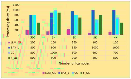
Figure 2. Number of fog nodes versus processing delay (ms).

6.2. Energy Consumption

A graph of the number of IoT requests versus energy consumption is shown in Figure 3. It is observed from the graph that the energy consumption of LLM_QL is consistently less (150–200 J) with the increase in the number of requests. The LLM-generated heuristic value is used for reward shaping, which helps in generating desired policy. The energy consumption of BAY_L and CC are found to be moderate (800–900 J). The centralized controller makes the system vulnerable and the presence of uncertainty is not handled in a generalized manner, whereas the energy consumption of F_QL is found to be very high (600–1000 J) with the increasing number of requests. With the increase in the state space, the Q-table becomes larger and maintenance becomes practically impossible.

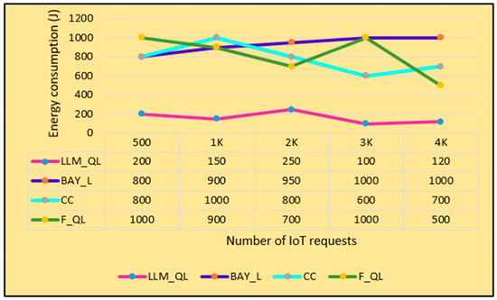
Figure 3. Number of IoT requests versus energy consumption (J).

6.3. Load Imbalance

The graph of the number of IoT requests versus load imbalance is shown in Figure 4. It is observed from the graph that the imbalance is less (0.2–0.4) for LLM_QL over the increase in the number of requests. Because of LLM guidance, there is no need for hyperparameter tuning and it can adapt quickly to different fog environment settings. The load imbalances of CC and F_QL are moderate (0.2–0.5) as the lookup table of Q state is replaced with the fuzzy system, which represents the state and action pair for each Q state. In contrast, the load balance of BAY_QL is found to be consistently very high (0.8–0.9) over the increase in the number of requests as it incorporates the previous beliefs, which results in an urge to converge to suboptimal solutions.

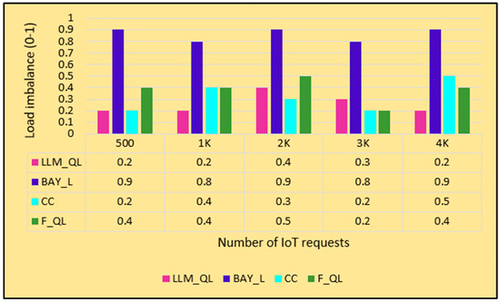
Figure 4. Number of IoT requests versus load imbalance (0–1).

6.4. Service Level Agreement Violation

A graph of time versus SLA violation is shown in Figure 5. It is observed from the graph that the SLA violation of LLM_QL is consistently less (5–10%) with respect to time as it prevents the overestimation and underestimation of Q values by nullifying the effect of hallucinations. The SLA violation of CC is moderate (20–80%) as it is properly streamlined and has a well-defined hierarchy system to ensure proper policy decisions. In contrast, the SLA violations of BAY_L and F_QL are high (20–90%) with respect to time because the rules are updated using the maximum operator, which is subject to positive bias and affects the learning process. Also, the computation cost is higher and the accuracy of the results varies depending on the value of the random seed used.

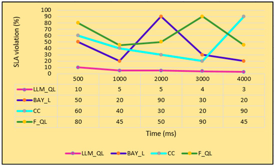
Figure 5. Time (ms) versus SLA violation (%).

7. Conclusions

This paper presents a novel LLM-guided Q-learning framework for resource provisioning in fog computing. The uncertainty in fog computing is modeled using an LLM model. The heuristic value of the LLM model is used to provide guidance to the Q-learning agent. Over and under provisioning of resources is prevented through proper exploration of the state space using the maximum entropy solution. The expected value analysis of the framework under finite and infinite fog computing scenarios is performed. The experimental results obtained by the iFogSim 3.3. simulator are good with respect to processing delay, load balancing, and SLA violations. As future work, detailed analytical modeling and analysis of the framework will be carried out in terms of resource migration and placement. Extension of the framework will be conducted pertaining to fault tolerance, auto recovery, and cost optimization.

References

- Srirama, S.N. A decade of research in fog computing: Relevance, challenges, and future directions. Softw. Pract. Exp. 2024, 54, 3–23. [Google Scholar] [CrossRef]
- Ali, S.; Alubady, R. A Survey of Fog Computing-Based Resource Allocation Approaches: Overview, Classification, and Opportunity for Research. Iraqi J. Sci. 2024, 65, 4008–4029. [Google Scholar] [CrossRef]
- Das, R.; Inuwa, M.M. A review on fog computing: Issues, characteristics, challenges, and potential applications. Telemat. Inform. Rep. 2023, 10, 100049. [Google Scholar] [CrossRef]
- Sabireen, H.; Neelanarayanan, V.J.I.E. A review on fog computing: Architecture, fog with IoT, algorithms and research challenges. Ict Express 2021, 7, 162–176. [Google Scholar]
- Clifton, J.; Laber, E. Q-learning: Theory and applications. Annu. Rev. Stat. Its Appl. 2020, 7, 279–301. [Google Scholar] [CrossRef]
- Hansen-Estruch, P.; Kostrikov, I.; Janner, M.; Kuba, J.G.; Levine, S. IDQL: Implicit q-learning as an actor-critic method with diffusion policies. arXiv 2023, arXiv:2304.10573. [Google Scholar]
- Zhao, W.X.; Zhou, K.; Li, J.; Tang, T.; Wang, X.; Hou, Y.; Wen, J.R. A survey of large language models. arXiv 2023, arXiv:2303.18223. [Google Scholar]
- Chang, Y.; Wang, X.; Wang, J.; Wu, Y.; Yang, L.; Zhu, K.; Xie, X. A survey on evaluation of large language models. ACM Trans. Intell. Syst. Technol. 2024, 15, 1–45. [Google Scholar] [CrossRef]
- Du, Y.; Watkins, O.; Wang, Z.; Colas, C.; Darrell, T.; Abbeel, P.; Andreas, J. Guiding pretraining in reinforcement learning with large language models. In Proceedings of the International Conference on Machine Learning, Honolulu, HI, USA, 23–29 July 2023; PMLR: New York, NY, USA, 2023; Volume 202, pp. 8657–8677. [Google Scholar]
- Ma, R.; Luijkx, J.; Ajanovic, Z.; Kober, J. ExploRLLM: Guiding exploration in reinforcement learning with large language models. arXiv 2024, arXiv:2403.09583. [Google Scholar]
- Abu-Amssimir, N.; Al-Haj, A. A QoS-aware resource management scheme over fog computing infrastructures in IoT systems. Multimed. Tools Appl. 2023, 82, 28281–28300. [Google Scholar] [CrossRef]
- Etemadi, M.; Ghobaei-Arani, M.; Shahidinejad, A. Resource provisioning for IoT services in the fog computing environment: An autonomic approach. Comput. Commun. 2020, 161, 109–131. [Google Scholar] [CrossRef]
- Nguyen, N.D.; Phan, L.A.; Park, D.H.; Kim, S.; Kim, T. ElasticFog: Elastic resource provisioning in container-based fog computing. IEEE Access 2020, 8, 183879–183890. [Google Scholar] [CrossRef]
- Mseddi, A.; Jaafar, W.; Elbiaze, H.; Ajib, W. Centralized and collaborative RL-based resource allocation in virtualized dynamic fog computing. IEEE Internet Things J. 2023, 10, 14239–14253. [Google Scholar] [CrossRef]
- Faraji-Mehmandar, M.; Jabbehdari, S.; Javadi, H.H.S. Fuzzy Q-learning approach for autonomic resource provisioning of IoT applications in fog computing environments. J. Ambient. Intell. Humaniz. Comput. 2023, 14, 4237–4255. [Google Scholar] [CrossRef]
- Etemadi, M.; Ghobaei-Arani, M.; Shahidinejad, A. A learning-based resource provisioning approach in the fog computing environment. J. Exp. Theor. Artif. Intell. 2021, 33, 1033–1056. [Google Scholar] [CrossRef]
- Sumona, S.T.; Hasan, S.S.; Tamzid, A.Y.; Roy, P.; Razzaque, M.A.; Mahmud, R. A Deep Q-Learning Framework for Enhanced QoE and Energy Optimization in Fog Computing. In Proceedings of the 2024 20th International Conference on Distributed Computing in Smart Systems and the Internet of Things (DCOSS-IoT), Abu Dhabi, United Arab Emirates, 29 April–1 May 2024; IEEE: New York, NY, USA, 2024; pp. 669–676. [Google Scholar]
- Baneshi, S.; Varbanescu, A.L.; Pathania, A.; Akesson, B.; Pimentel, A. Estimating the energy consumption of applications in the computing continuum with ifogsim. In Proceedings of the International Conference on High Performance Computing, Denver, CO, USA, 12–17 November 2023; Springer Nature: Cham, Switzerland, 2023; pp. 234–249. [Google Scholar]
- Mahmud, R.; Pallewatta, S.; Goudarzi, M.; Buyya, R. Ifogsim2: An extended ifogsim simulator for mobility, clustering, and microservice management in edge and fog computing environments. J. Syst. Softw. 2022, 190, 111351. [Google Scholar] [CrossRef]
- Kocon, J.; Cichecki, I.; Kaszyca, O.; Kochanek, M.; Szydło, D.; Baran, J.; Kazienko, P. ChatGPT: Jack of all trades, master of none. Inf. Fusion 2023, 99, 101861. [Google Scholar] [CrossRef]
- Vujinović, A.; Luburić, N.; Slivka, J.; Kovačević, A. Using ChatGPT to annotate a dataset: A case study in intelligent tutoring systems. Mach. Learn. Appl. 2024, 16, 100557. [Google Scholar] [CrossRef]
- Pandey, C.; Tiwari, V.; Rathore, R.S.; Jhaveri, R.H.; Roy, D.S.; Selvarajan, S. Resource-efficient synthetic data generation for performance evaluation in mobile edge computing over 5G networks. IEEE Open J. Commun. Soc. 2023, 4, 1866–1878. [Google Scholar] [CrossRef]
Disclaimer/Publisher’s Note: The statements, opinions and data contained in all publications are solely those of the individual author(s) and contributor(s) and not of MDPI and/or the editor(s). MDPI and/or the editor(s) disclaim responsibility for any injury to people or property resulting from any ideas, methods, instructions or products referred to in the content. |
© 2025 by the authors. Licensee MDPI, Basel, Switzerland. This article is an open access article distributed under the terms and conditions of the Creative Commons Attribution (CC BY) license (https://creativecommons.org/licenses/by/4.0/).