Robust Regularized Recursive Least-Squares Algorithm Based on Third-Order Tensor Decomposition

Abstract

The decomposition-based adaptive filtering algorithms have recently gained increasing interest due to their capability to reduce the parameter space. In this context, the third-order tensor (TOT) decomposition technique reformulates the conventional approach that involves a single (usually long) adaptive filter by using a combination of three shorter filters via the Kronecker product. This leads to a twofold gain in terms of both performance and complexity. Thus, it can be applied efficiently when operating with more complex algorithms, like the recursive least-squares (RLS) approach. In this paper, we develop an RLS-TOT algorithm with improved robustness features due to a novel regularization method that considers the contribution of the external noise and the so-called model uncertainties (which are related to the system). Simulation results obtained in the framework of echo cancelation support the performance of the proposed algorithm, which outperforms the existing RLS-TOT counterparts, as well as the conventional RLS algorithm that uses the specific regularization technique.

1. Introduction

In many real-world applications, adaptive filters of all sorts play a fundamental role [1]. Basically, such an adaptive system consists of a digital filter with time-varying coefficients, which are updated based on an iterative method, also known as the adaptive algorithm [2]. The choice of a particular adaptive algorithm for a specific application depends on several performance criteria, like the convergence rate, solution accuracy, robustness capability, and computational efficiency. While the least-mean-square (LMS) algorithm remains one of the most popular choices due to its simplicity, the improved performance features support using the recursive least-squares (RLS) algorithm for nowadays applications [3].

The length of the adaptive filter (i.e., the number of coefficients) is a critical factor related to the practical implementation of such a system. The longer the filter, the more challenging its implementation/operation becomes. This aspect is not only associated with the computational complexity, which naturally increases with the number of coefficients, but also with the main performance criteria. A longer filter implies a slower convergence rate and tracking while also influencing the accuracy of the solution. Since there are many applications that require adaptive filters with hundreds of coefficients (e.g., echo cancelation, channel modeling, noise reduction, etc.), dealing with such long-length impulse responses represents an important challenge, especially in conjunction with the RLS-based algorithms [4,5].

Recent works have addressed this problem by focusing on impulse response decomposition techniques, which aim to reformulate a problem with a large parameter space (i.e., a large number of filter coefficients) as a combination of “smaller” problems, i.e., shorter filters [6,7,8,9,10,11,12]. In this framework, one of the most appealing solutions relies on the nearest Kronecker product (NKP) decomposition of the impulse response, which exploits the low-rank features that characterize most of the real-world systems [13,14,15,16,17,18,19,20,21].

The basis of the NKP approach was developed in the context of a second-order decomposition [13,14], where an impulse response of length $L=L_1{L}_2$ (with $L_2\le L_1$) is approximated by a sum of R Kronecker products (with $R\ll L_2$) between shorter impulse responses of lengths $L_2$ and $L_1$. In fact, R is the approximated rank of the $L_1\times L_2$ matrix that results from reshaping the impulse response of length L. Apparently, a higher-order decomposition is desirable since it would involve even shorter impulse responses. Nevertheless, in this case, the impulse response would be reshaped as a higher-order tensor, while the rank of such a structure is not always straightforward to handle [22,23,24]. The solution proposed in [20] avoids this issue and controls a third-order tensor’s rank via a matrix rank. As a result, the RLS-based algorithm using such a third-order tensor (TOT) decomposition, namely RLS-TOT [21], outperforms its previously developed counterpart that exploits the second-order NKP decomposition [14].

Besides the previously mentioned performance criteria (e.g., convergence, tracking, and accuracy), there is another important aspect that should be taken into account when the system operates in noisy environments. In such scenarios, the robustness of the adaptive algorithm becomes a critical issue. For example, in echo cancelation, the microphone captures the background noise, which could be strong and nonstationary. Consequently, its presence could significantly bias the adaptive filter behavior if the algorithm is not equipped with strong robustness features. Usually, the robustness of the algorithm is considered in the design phase by including specific terms into the optimization cost function [25,26,27,28,29,30]. Nevertheless, the resulting regularized algorithms frequently include additional parameters that are not always easy to control in practice. In this context, the solution recently proposed in [31] considers a cost function that includes the contribution of both the external noise and the system uncertainties, while the variances of these terms are estimated in a practical manner within the algorithm.

The RLS-TOT algorithm developed in [21] exploits the TOT-based decomposition of the global impulse response of the filter (which could have a large number of coefficients). As a result, it solves the associated system identification problem by combining the estimates provided by three (usually much shorter) adaptive filters. Consequently, the resulting gain is twofold, in terms of performance assets (e.g., faster tracking and better accuracy) and lower computational complexity. However, the cost functions related to the three component filters follow the line of the conventional RLS algorithm and do not include any regularization component. Thus, the so-called forgetting factors [21] remain the only control parameters of this TOT-based algorithm, so that its robustness is inherently limited in noisy environments.

Recently, a robust RLS-type algorithm was developed in [31], following the line of the conventional RLS version (without decomposition), but including a proper regularization term within the cost function. This regularization technique considers the influence of two important factors that could significantly influence the overall performance in real-world environments. First, it includes the external noise power, which is further estimated in a practical manner within the regularized RLS-type algorithm (based on the error signal). Second, it considers the so-called model “uncertainties” [31], which are related to the variability of the unknown system to be identified. The resulting parameter can also be estimated in a practical way by using a measure related to the Euclidean norm of the difference between the estimates provided by the adaptive filter from two consecutive moments of time. As a result, the algorithm proposed in [31] has a significantly improved robustness in noisy conditions, as compared to the non-regularized counterparts. Nevertheless, it does not involve any decomposition-based technique; thus, it still faces the inherent challenges related to the identification of long impulse responses.

Motivated by these aspects, in this article, we follow the idea from [31] in order to develop a regularized version of the RLS-TOT algorithm, with improved robustness features compared to its counterpart from [21]. As a result, the proposed algorithm inherits the advantages of the decomposition-based approach and the robust behavior due to the regularization technique. Following this introduction, the TOT-based decomposition is presented in Section 2. Then, the proposed regularized RLS-TOT algorithm is developed in Section 3. The experimental scenario presented in Section 4 considers an echo cancelation application, and the obtained results support the performance features of the proposed solution. A brief discussion related to the strengths and limitations of the regularized RLS-TOT algorithm, together with some potential extensions, is provided in Section 5. The paper concludes in Section 6, also outlining several perspectives for future research.

2. TOT Decomposition

In this section, the background behind the TOT decomposition is presented, together with the specific framework and notation. Let us consider a time-varying system characterized by the impulse response of length L, denoted by the vector:

$$\begin{array}{c}\hfill \mathbf{h}\left(n\right)={\left[\begin{array}{cccc}{h}_1\left(n\right)& h_2\left(n\right)& \cdots & h_L\left(n\right)\end{array}\right]}^{\top },\end{array}$$

(1)

where n represents the discrete-time index, $h_l\left(n\right)$ is the lth coefficient (with $l=1,2,\dots ,L$), and the superscript ^⊤ stands for transposition. Next, it is assumed that the length can be factorized as $L=L_1{L}_2$, with $L_1\ge L_2$. This may not seem like a trivial assumption, but in many finite-precision implementations, the length of a digital filter is usually set as a power of two (for practical/algorithmic reasons), i.e., $L=2^B$, where B is a positive integer. Consequently, it can be easily factorized as $L=2^{B_1}{2}^{B_2}$, with $B=B_1+B_2$ and $B_1\ge B_2$ (where $B_1$ and $B_2$ are also positive integers).

Using the Kronecker product, the impulse response from (1) can be equivalently expressed as [13]

$$\begin{array}{cc}\hfill \mathbf{h}\left(n\right)& =\sum _{i=1}^{L_2}{\mathbf{h}}_{2,i}\left(n\right)\otimes {\mathbf{h}}_{1,i}\left(n\right),\hfill \end{array}$$

(2)

where ${\mathbf{h}}_{2,i}\left(n\right)$ and ${\mathbf{h}}_{1,i}\left(n\right)$, with $i=1,2,\dots ,L_2$, are shorter impulse responses of lengths $L_2$ and $L_1$, respectively, while ⊗ denotes the Kronecker product [32]. As shown in [13], the coefficients of these shorter impulse responses can be evaluated using the singular value decomposition (SVD) of the matrix $\mathbf{H}\left(n\right)$, of size $L_1\times L_2$, which is obtained by reshaping the elements of $\mathbf{h}\left(n\right)$. Nevertheless, in terms of the parameter space, there is no reason to use (2) instead of (1), since the former involves $L_2(L_2+L_1)=L_2^2+L$ coefficients, which exceed the length L associated with (1). However, for low-rank systems, i.e., the rank of $\mathbf{H}\left(n\right)$ is smaller than $L_2$, there is a potential gain. Indeed, let us denote by R the rank of $\mathbf{H}\left(n\right)$, with $R<L_2$. In this case, using the NKP decomposition [13], (2) becomes

$$\begin{array}{cc}\hfill \mathbf{h}\left(n\right)& =\sum _{r=1}^R{\mathbf{h}}_{2,r}\left(n\right)\otimes {\mathbf{h}}_{1,r}\left(n\right),\hfill \end{array}$$

(3)

where ${\mathbf{h}}_{2,r}\left(n\right)$ and ${\mathbf{h}}_{1,r}\left(n\right)$, with $r=1,2,\dots ,R$, are impulse responses of lengths $L_2$ and $L_1$, respectively. Thus, the parameter space consists of $R(L_2+L_1)$ coefficients, a number that can be significantly smaller than L. In fact, in many practical scenarios (e.g., echo cancelation, noise reduction, etc.), the setup is $R\ll L_2$ [13,14], thus leading to important advantages.

Apparently, increasing the decomposition order would be a benefit in terms of reducing the parameter space. In this case, the length L would be factorized in more than two terms, while more than two (even shorter) impulse responses would be combined via the Kronecker product in the decomposition of $\mathbf{h}\left(n\right)$, similar to (2). Nevertheless, the number of terms in the sum would not be related to a matrix rank anymore, but to a tensor rank, which is a more sensitive issue [22,23,24]. For example, while the rank of a matrix is limited by the number of its columns, a tensor rank could exceed the largest dimension of its decomposition.

In order to avoid such shortcomings, the TOT-based solution from [20] starts with the factorization $L=L_1{L}_2$, but considering that $L_1\gg L_2$, while also decomposing $L_1=L_{11}{L}_{12}$, with $L_{11}\ge L_{12}$. Then, following the same low-rank framework, the decomposition of the impulse response results in [20]

$$\begin{array}{cc}\hfill \mathbf{h}\left(n\right)& =\sum _{l=1}^{L_2}\sum _{p=1}^P{\mathbf{h}}_{2,l}\left(n\right)\otimes {\mathbf{h}}_{12,lp}\left(n\right)\otimes {\mathbf{h}}_{11,lp}\left(n\right),\hfill \end{array}$$

(4)

with $P<L_{12}$, and the shorter impulse responses ${\mathbf{h}}_{2,l}\left(n\right)$, ${\mathbf{h}}_{12,lp}\left(n\right)$, and ${\mathbf{h}}_{11,lp}\left(n\right)$ having the lengths $L_2$, $L_{12}$, and $L_{11}$, respectively. Hence, according to (4), the parameter space becomes $L_2^2+P{L}_{12}{L}_2+P{L}_{11}{L}_2$, which can be significantly smaller than L, under the common settings $L_2\ll L_{11}{L}_{12}$ and $P\ll L_{12}$ [20,21].

To facilitate the upcoming developments, the coefficients of the component impulse responses from (4) are grouped into the following data structures, which are specific to the TOT decomposition:

$$\begin{array}{cc}\hfill {\underline{\mathbf{h}}}_2\left(n\right)& =\left[\begin{array}{c}{\mathbf{h}}_{2,1}\left(n\right)\hfill \\ {\mathbf{h}}_{2,2}\left(n\right)\hfill \\ ⋮\hfill \\ {\mathbf{h}}_{2,L_2}\left(n\right)\hfill \end{array}\right],\hfill \end{array}$$

(5)

$$\begin{array}{cc}\hfill {\overline{\underline{\mathbf{h}}}}_{12}\left(n\right)& =\left[\begin{array}{c}{\overline{\mathbf{h}}}_{12,1}\left(n\right)\hfill \\ {\overline{\mathbf{h}}}_{12,2}\left(n\right)\hfill \\ ⋮\hfill \\ {\overline{\mathbf{h}}}_{12,L_2}\left(n\right)\hfill \end{array}\right],{\overline{\mathbf{h}}}_{12,l}\left(n\right)=\left[\begin{array}{c}{\mathbf{h}}_{12,1}\left(n\right)\hfill \\ {\mathbf{h}}_{12,2}\left(n\right)\hfill \\ ⋮\hfill \\ {\mathbf{h}}_{12,P}\left(n\right)\hfill \end{array}\right],\hfill \end{array}$$

(6)

$$\begin{array}{cc}\hfill {\overline{\underline{\mathbf{h}}}}_{11}\left(n\right)& =\left[\begin{array}{c}{\overline{\mathbf{h}}}_{11,1}\left(n\right)\hfill \\ {\overline{\mathbf{h}}}_{11,2}\left(n\right)\hfill \\ ⋮\hfill \\ {\overline{\mathbf{h}}}_{11,L_2}\left(n\right)\hfill \end{array}\right],{\overline{\mathbf{h}}}_{11,l}\left(n\right)=\left[\begin{array}{c}{\mathbf{h}}_{11,1}\left(n\right)\hfill \\ {\mathbf{h}}_{11,2}\left(n\right)\hfill \\ ⋮\hfill \\ {\mathbf{h}}_{11,P}\left(n\right)\hfill \end{array}\right],\hfill \end{array}$$

(7)

with $l=1,2,\dots ,L_2$. It should also be noticed that the terms that compose the sums in (4) can be equivalently expressed as

$$\begin{array}{cc}\hfill {\mathbf{h}}_{2,l}\left(n\right)\otimes {\mathbf{h}}_{12,lp}\left(n\right)\otimes {\mathbf{h}}_{11,lp}\left(n\right)& =\left[{\mathbf{I}}_{L_2}\otimes {\mathbf{h}}_{12,lp}\left(n\right)\otimes {\mathbf{h}}_{11,lp}\left(n\right)\right]{\mathbf{h}}_{2,l}\left(n\right)\hfill \end{array}$$

(8)

$$\begin{array}{cc}\hfill & =\left[{\mathbf{h}}_{2,l}\left(n\right)\otimes {\mathbf{I}}_{L_{12}}\otimes {\mathbf{h}}_{11,lp}\left(n\right)\right]{\mathbf{h}}_{12,lp}\left(n\right)\hfill \end{array}$$

(9)

$$\begin{array}{cc}\hfill & =\left[{\mathbf{h}}_{2,l}\left(n\right)\otimes {\mathbf{h}}_{12,lp}\left(n\right)\otimes {\mathbf{I}}_{L_{11}}\right]{\mathbf{h}}_{11,lp}\left(n\right),\hfill \end{array}$$

(10)

where ${\mathbf{I}}_{L_2}$, ${\mathbf{I}}_{L_{12}}$, and ${\mathbf{I}}_{L_{11}}$ denote the identity matrices of size $L_2\times L_2$, $L_{12}\times L_{12}$, and $L_{11}\times L_{11}$, respectively. These equivalent forms are useful to further extract the individual components of the global impulse response, i.e., the last terms that appear in the right-hand side of (8), (9), and (10), respectively. In fact, these sets of coefficients compose the impulse responses from (5)–(7), i.e., ${\underline{\mathbf{h}}}_2\left(n\right)$, ${\overline{\underline{\mathbf{h}}}}_{12}\left(n\right)$, and ${\overline{\underline{\mathbf{h}}}}_{11}\left(n\right)$, which have the lengths $L_2^2$, $P{L}_{12}{L}_2$, and $P{L}_{11}{L}_2$, respectively. Concluding, the adaptive filters that exploit the TOT-based decomposition are designed to estimate these three component impulse responses, instead of directly modeling the global impulse response of length L. Furthermore, the coefficients of the estimated (full-length) impulse response can be obtained similarly to (4), as will be shown in the next section.

3. RLS-TOT Algorithm and Its Regularized Version

An adaptive filter consists of a digital filter controlled by an iterative algorithm, which updates its coefficients in order to minimize a certain cost function that depends on the error signal [1,2,3]. This error is defined as the difference between a reference (or desired) signal, $d\left(n\right)$, and the output of the adaptive filter. Let us consider that the reference signal is obtained at the output of an unknown system, which is defined by the impulse response $\mathbf{h}\left(n\right)$ of length L, as introduced at the beginning of Section 2. Also, it is considered that a zero-mean additive noise, $v\left(n\right)$, corrupts this output, so that the reference signal results in

$$\begin{array}{cc}\hfill d\left(n\right)& ={\mathbf{x}}^{\top }\left(n\right)\mathbf{h}\left(n\right)+v\left(n\right),\hfill \end{array}$$

(11)

where

$$\begin{array}{cc}\hfill \mathbf{x}\left(n\right)& ={\left[\begin{array}{cccc}x\left(n\right)& x(n-1)& \dots & x(n-L+1)\end{array}\right]}^{\top }\hfill \end{array}$$

(12)

contains the most recent L samples of the zero-mean input signal $x\left(n\right)$, which is independent of $v\left(n\right)$. This signal also drives the input of the adaptive filter, with the objective of identifying the unknown impulse response and delivering its estimate, denoted by $\widehat{\mathbf{h}}\left(n\right)$. Consequently, the a priori error signal is evaluated using the estimated coefficients from time index $n-1$, i.e.,

$$\begin{array}{cc}\hfill e\left(n\right)& =d\left(n\right)-{\mathbf{x}}^{\top }\left(n\right)\widehat{\mathbf{h}}(n-1),\hfill \end{array}$$

(13)

while the common form of the filter update is

$$\begin{array}{cc}\hfill \widehat{\mathbf{h}}\left(n\right)& =\widehat{\mathbf{h}}(n-1)+\mathcal{U}\left[\mathbf{x}\left(n\right),e\left(n\right)\right],\hfill \end{array}$$

(14)

where $\mathcal{U}\left[\mathbf{x}\left(n\right),e\left(n\right)\right]$ generally denotes the update term, which depends on the input vector and the error signal. This update term results in different forms, depending on the adaptive filtering algorithm.

In this framework, the least-squares (LS) optimization criterion [1,2,3] represents one of the most reliable approaches, which targets the minimization of the cost function:

$$\begin{array}{cc}\hfill \mathcal{J}\left(n\right)& =\sum _{i=1}^n{\lambda }^{n-i}{\left[d\left(i\right)-{\mathbf{x}}^{\top }\left(i\right)\widehat{\mathbf{h}}\left(n\right)\right]}^2,\hfill \end{array}$$

(15)

with respect to $\widehat{\mathbf{h}}\left(n\right)$, where $\lambda$ represents the forgetting factor ($0<\lambda \le 1$). Following this approach, the normal equations to be solved result in

$$\begin{array}{cc}\hfill \mathbf{R}\left(n\right)\widehat{\mathbf{h}}\left(n\right)& =\mathbf{r}\left(n\right),\hfill \end{array}$$

(16)

where

$$\begin{array}{cc}\hfill \mathbf{R}\left(n\right)& =\lambda \mathbf{R}(n-1)+\mathbf{x}\left(n\right){\mathbf{x}}^{\top }\left(n\right),\hfill \end{array}$$

(17)

$$\begin{array}{cc}\hfill \mathbf{r}\left(n\right)& =\lambda \mathbf{r}(n-1)+\mathbf{x}\left(n\right)d\left(n\right).\hfill \end{array}$$

(18)

The solution can be formulated in a recursive manner, which leads to the well-known RLS algorithm that is defined by the update relation [1,2,3]:

$$\begin{array}{cc}\hfill \widehat{\mathbf{h}}\left(n\right)& =\widehat{\mathbf{h}}(n-1)+{\mathbf{R}}^{-1}\left(n\right)\mathbf{x}\left(n\right)e\left(n\right),\hfill \end{array}$$

(19)

where $e\left(n\right)$ is the a priori error signal defined in (13). In this context, $\mathbf{R}\left(n\right)$ from (17) represents an estimate of the input signal covariance matrix.

There are different versions of the RLS algorithm that avoid a direct matrix inversion in (19), e.g., by using the matrix inversion lemma (also known as the Woodbury formula) [1,2,3] or the line search methods [33,34,35,36,37]. The first approach leads to the most popular version of the RLS algorithm, in which the inverse of $\mathbf{R}\left(n\right)$ is recursively updated. The computational amount required by this version is proportional to $\mathcal{O}\left(L^2\right)$. Nevertheless, the second approach that exploits the line search methods is more advantageous in terms of computational complexity. In this case, following (19), the filter update is rewritten as $\widehat{\mathbf{h}}\left(n\right)=\widehat{\mathbf{h}}(n-1)+\Delta \widehat{\mathbf{h}}\left(n\right)$, where the “increment” (i.e., the update term) results as the iterative solution of an auxiliary set of normal equations, $\mathbf{R}\left(n\right)\Delta \widehat{\mathbf{h}}\left(n\right)=\mathbf{p}\left(n\right)$, where $\mathbf{p}\left(n\right)=\lambda \mathbf{p}(n-1)+\mathbf{x}\left(n\right)e\left(n\right)$ is the so-called residual vector. Among these iterative techniques, the dichotomous coordinate descent (DCD) method proposed by Zakharov et al. [34] stands out as the most representative, which leads to a computational complexity of the resulting RLS-DCD algorithm proportional to $\mathcal{O}\left(L\right)$. In this context, we should note that different “fast” RLS algorithms can be found in the literature, for various filter structures [1,2,3,5]. Their analysis is beyond the scope of this paper, which follows the basic form of the RLS-based update from (19), for the sake of generality.

In the context of the TOT-based decomposition presented in Section 2, the estimate provided by the adaptive filter can be decomposed into a form similar to (4), i.e.,

$$\begin{array}{cc}\hfill \widehat{\mathbf{h}}\left(n\right)& =\sum _{l=1}^{L_2}\sum _{p=1}^P{\widehat{\mathbf{h}}}_{2,l}\left(n\right)\otimes {\widehat{\mathbf{h}}}_{12,lp}\left(n\right)\otimes {\widehat{\mathbf{h}}}_{11,lp}\left(n\right),\hfill \end{array}$$

(20)

where the impulse responses ${\widehat{\mathbf{h}}}_{2,l}\left(n\right)$, ${\widehat{\mathbf{h}}}_{12,lp}\left(n\right)$, and ${\widehat{\mathbf{h}}}_{11,lp}\left(n\right)$ have the lengths $L_2$, $L_{12}$, and $L_{11}$, respectively. Furthermore, similar to (5)–(7), we can obtain the component filters ${\widehat{\underline{\mathbf{h}}}}_2\left(n\right)$, ${\widehat{\overline{\underline{\mathbf{h}}}}}_{12}\left(n\right)$, and ${\widehat{\overline{\underline{\mathbf{h}}}}}_{11}\left(n\right)$, of lengths $L_2^2$, $P{L}_{12}{L}_2$, and $P{L}_{11}{L}_2$, respectively. As a result, based on the properties of the Kronecker product, like in (8)–(10), each of these three component filters can be processed separately [20,21].

First, focusing on ${\widehat{\underline{\mathbf{h}}}}_2\left(n\right)$, which contains the taps of ${\widehat{\mathbf{h}}}_{2,l}\left(n\right)$, with $l=1,2,\dots ,L_2$, the other two sets of coefficients can be grouped into the following matrices:

$$\begin{array}{cc}\hfill {\widehat{\mathbf{H}}}_{12,11,lp}\left(n\right)& ={\mathbf{I}}_{L_2}\otimes {\widehat{\mathbf{h}}}_{12,lp}\left(n\right)\otimes {\widehat{\mathbf{h}}}_{11,lp}\left(n\right),\hfill \\ \hfill {\widehat{\overline{\mathbf{H}}}}_{12,11,l}\left(n\right)& =\sum _{p=1}^P{\widehat{\mathbf{H}}}_{12,11,lp}\left(n\right),\hfill \\ \hfill {\widehat{\underline{\overline{\mathbf{H}}}}}_{12,11}\left(n\right)& =\left[\begin{array}{cccc}{\widehat{\overline{\mathbf{H}}}}_{12,11,1}\left(n\right)& {\widehat{\overline{\mathbf{H}}}}_{12,11,2}\left(n\right)& \dots & {\widehat{\overline{\mathbf{H}}}}_{12,11,L_2}\left(n\right)\end{array}\right],\hfill \end{array}$$

where $p=1,2,\dots ,P$. Consequently, a cost function similar to (15) can be formulated as

$$\begin{array}{cc}\hfill {\mathcal{J}}_2\left(n\right)& =\sum _{i=1}^n{\lambda }_2^{n-i}{\left[d\left(i\right)-{\mathbf{x}}^{\top }\left(i\right){\widehat{\underline{\overline{\mathbf{H}}}}}_{12,11}\left(i\right){\widehat{\underline{\mathbf{h}}}}_2\left(n\right)\right]}^2,\hfill \end{array}$$

(21)

where $0<{\lambda }_2\le 1$ is a forgetting factor. The minimization of ${\mathcal{J}}_2\left(n\right)$ with respect to ${\widehat{\underline{\mathbf{h}}}}_2\left(n\right)$ relies on a multilinear optimization strategy [38], which considers that the other two component filters are fixed. Following similar steps that led to (16)–(19) and introducing the notation ${\mathbf{x}}_{12,11}\left(n\right)={\widehat{\underline{\overline{\mathbf{H}}}}}_{12,11}^{\top }(n-1)\mathbf{x}\left(n\right)$, the relations that define the RLS-based algorithm associated with this component filter result in

$$\begin{array}{cc}\hfill {\mathbf{R}}_{12,11}\left(n\right)& ={\lambda }_2{\mathbf{R}}_{12,11}(n-1)+{\mathbf{x}}_{12,11}\left(n\right){\mathbf{x}}_{12,11}^{\top }\left(n\right),\hfill \end{array}$$

(22)

$$\begin{array}{cc}\hfill e_2\left(n\right)& =d\left(n\right)-{\mathbf{x}}_{12,11}^{\top }\left(n\right){\widehat{\underline{\mathbf{h}}}}_2(n-1),\hfill \end{array}$$

(23)

$$\begin{array}{cc}\hfill {\widehat{\underline{\mathbf{h}}}}_2\left(n\right)& ={\widehat{\underline{\mathbf{h}}}}_2(n-1)+{\mathbf{R}}_{12,11}^{-1}\left(n\right){\mathbf{x}}_{12,11}\left(n\right)e_2\left(n\right).\hfill \end{array}$$

(24)

In a similar manner, the optimization process is carried out for the second component filter, ${\widehat{\overline{\underline{\mathbf{h}}}}}_{12}\left(n\right)$, which groups the taps of ${\widehat{\mathbf{h}}}_{12,lp}\left(n\right)$, with $l=1,2\dots ,L_2$ and $p=1,2\dots ,P$. Starting with the notation:

$$\begin{array}{cc}\hfill {\widehat{\mathbf{H}}}_{2,11,lp}\left(n\right)& ={\widehat{\mathbf{h}}}_{2,l}\left(n\right)\otimes {\mathbf{I}}_{L_{12}}\otimes {\widehat{\mathbf{h}}}_{11,lp}\left(n\right),\hfill \\ \hfill {\widehat{\overline{\mathbf{H}}}}_{2,11,l}\left(n\right)& =\left[\begin{array}{cccc}{\widehat{\mathbf{H}}}_{2,11,l1}\left(n\right)& {\widehat{\mathbf{H}}}_{2,11,l2}\left(n\right)& \dots & {\widehat{\mathbf{H}}}_{2,11,lP}\left(n\right)\end{array}\right],\hfill \\ \hfill {\widehat{\underline{\overline{\mathbf{H}}}}}_{2,11}\left(n\right)& =\left[\begin{array}{cccc}{\widehat{\overline{\mathbf{H}}}}_{2,11,1}\left(n\right)& {\widehat{\overline{\mathbf{H}}}}_{2,11,2}\left(n\right)& \dots & {\widehat{\overline{\mathbf{H}}}}_{2,11,L_2}\left(n\right)\end{array}\right],\hfill \end{array}$$

the related cost function becomes

$$\begin{array}{cc}\hfill {\mathcal{J}}_{12}\left(n\right)& =\sum _{i=1}^n{\lambda }_{12}^{n-i}{\left[d\left(i\right)-{\mathbf{x}}^{\top }\left(i\right){\widehat{\underline{\overline{\mathbf{H}}}}}_{2,11}\left(i\right){\widehat{\overline{\underline{\mathbf{h}}}}}_{12}\left(n\right)\right]}^2,\hfill \end{array}$$

(25)

with the associated forgetting factor $0<{\lambda }_{12}\le 1$. Using the same multilinear optimization strategy, the RLS-type algorithm for the second component filter is defined by the following relations:

$$\begin{array}{cc}\hfill {\mathbf{R}}_{2,11}\left(n\right)& ={\lambda }_{12}{\mathbf{R}}_{2,11}(n-1)+{\mathbf{x}}_{2,11}\left(n\right){\mathbf{x}}_{2,11}^{\top }\left(n\right),\hfill \end{array}$$

(26)

$$\begin{array}{cc}\hfill e_{12}\left(n\right)& =d\left(n\right)-{\mathbf{x}}_{2,11}^{\top }\left(n\right){\widehat{\underline{\mathbf{h}}}}_{12}(n-1),\hfill \end{array}$$

(27)

$$\begin{array}{cc}\hfill {\widehat{\overline{\underline{\mathbf{h}}}}}_{12}\left(n\right)& ={\widehat{\overline{\underline{\mathbf{h}}}}}_{12}(n-1)+{\mathbf{R}}_{2,11}^{-1}\left(n\right){\mathbf{x}}_{2,11}\left(n\right)e_{12}\left(n\right),\hfill \end{array}$$

(28)

with ${\mathbf{x}}_{2,11}\left(n\right)={\widehat{\underline{\overline{\mathbf{H}}}}}_{2,11}^{\top }(n-1)\mathbf{x}\left(n\right)$.

The development of the third component filter follows the same path as the second one. The purpose is to update ${\widehat{\overline{\underline{\mathbf{h}}}}}_{11}\left(n\right)$, which contains the coefficients ${\widehat{\mathbf{h}}}_{11,lp}\left(n\right)$, with $l=1,2\dots ,L_2$ and $p=1,2\dots ,P$. Therefore, the associated notation is

$$\begin{array}{cc}\hfill {\widehat{\mathbf{H}}}_{2,12,lp}\left(n\right)& ={\widehat{\mathbf{h}}}_{2,l}\left(n\right)\otimes {\widehat{\mathbf{h}}}_{12,lp}\left(n\right)\otimes {\mathbf{I}}_{L_{11}},\hfill \\ \hfill {\widehat{\overline{\mathbf{H}}}}_{2,12,l}\left(n\right)& =\left[\begin{array}{cccc}{\widehat{\mathbf{H}}}_{2,12,l1}\left(n\right)& {\widehat{\mathbf{H}}}_{2,12,l2}\left(n\right)& \dots & {\widehat{\mathbf{H}}}_{2,12,lP}\left(n\right)\end{array}\right],\hfill \\ \hfill {\widehat{\underline{\overline{\mathbf{H}}}}}_{2,12}\left(n\right)& =\left[\begin{array}{cccc}{\widehat{\overline{\mathbf{H}}}}_{2,12,1}\left(n\right)& {\widehat{\overline{\mathbf{H}}}}_{2,12,2}\left(n\right)& \dots & {\widehat{\overline{\mathbf{H}}}}_{2,12,L_2}\left(n\right)\end{array}\right],\hfill \end{array}$$

which allows us to define the cost function

$$\begin{array}{cc}\hfill {\mathcal{J}}_{11}\left(n\right)& =\sum _{i=1}^n{\lambda }_{11}^{n-i}{\left[d\left(i\right)-{\mathbf{x}}^{\top }\left(i\right){\widehat{\underline{\overline{\mathbf{H}}}}}_{2,12}\left(i\right){\widehat{\overline{\underline{\mathbf{h}}}}}_{11}\left(n\right)\right]}^2,\hfill \end{array}$$

(29)

with the forgetting factor $0<{\lambda }_{11}\le 1$. Finally, the minimization of ${\mathcal{J}}_{11}\left(n\right)$ with respect to ${\widehat{\overline{\underline{\mathbf{h}}}}}_{11}\left(n\right)$, under the same multilinear optimization strategy, results in the associated RLS-based algorithm, which is defined by the relations:

$$\begin{array}{cc}\hfill {\mathbf{R}}_{2,12}\left(n\right)& ={\lambda }_{11}{\mathbf{R}}_{2,12}(n-1)+{\mathbf{x}}_{2,12}\left(n\right){\mathbf{x}}_{2,12}^{\top }\left(n\right),\hfill \end{array}$$

(30)

$$\begin{array}{cc}\hfill e_{11}\left(n\right)& =d\left(n\right)-{\mathbf{x}}_{2,12}^{\top }\left(n\right){\widehat{\underline{\mathbf{h}}}}_{11}(n-1),\hfill \end{array}$$

(31)

$$\begin{array}{cc}\hfill {\widehat{\overline{\underline{\mathbf{h}}}}}_{11}\left(n\right)& ={\widehat{\overline{\underline{\mathbf{h}}}}}_{11}(n-1)+{\mathbf{R}}_{2,12}^{-1}\left(n\right){\mathbf{x}}_{2,12}\left(n\right)e_{11}\left(n\right),\hfill \end{array}$$

(32)

where ${\mathbf{x}}_{2,12}\left(n\right)={\widehat{\underline{\overline{\mathbf{H}}}}}_{2,12}^{\top }(n-1)\mathbf{x}\left(n\right)$.

It can be noted that $e_2\left(n\right)=e_{12}\left(n\right)=e_{11}\left(n\right)=e\left(n\right)$, so that the a priori error from (13) is equivalent to the alternative expressions from (23), (27), and (31). Nevertheless, for the fluency of the development, these three alternative forms are used. On the other hand, the conventional form of the RLS algorithm, defined by (13), (17), and (19), is reformulated using the TOT-based decomposition as a combination of three shorter RLS-based filters, defined by (22)–(24), (26)–(28), and (30)–(32). This approach could lead to important advantages, in terms of both performance and complexity, as indicated in [21], where a version of the RLS-TOT based on the matrix inversion lemma was analyzed. However, this version is inherently limited in terms of robustness, since the only control parameters are the forgetting factors associated with the three component filters, i.e., ${\lambda }_2$, ${\lambda }_{12}$, and ${\lambda }_{11}$, respectively. Even when using the maximum values of these parameters (i.e., one), they cannot cope in noisy environments, with high and/or nonstationary noises. This is the main motivation for the upcoming development, which targets the derivation of a robust version of the RLS-TOT algorithm, using a recently designed regularization technique [31].

To this purpose, the cost functions from (21), (25), and (29) need to be adjusted by considering the weighted LS criterion and also including appropriate regularization terms [31]. Consequently, the proposed regularized RLS-TOT algorithm relies on the following modified cost functions:

$$\begin{array}{cc}\hfill {\underline{\mathcal{J}}}_2\left(n\right)& ={\displaystyle \frac{1}{{\sigma }_v^2}}{\mathcal{J}}_2\left(n\right)+{\mathcal{R}}_2\left(n\right),\hfill \end{array}$$

(33)

$$\begin{array}{cc}\hfill {\underline{\mathcal{J}}}_{12}\left(n\right)& ={\displaystyle \frac{1}{{\sigma }_v^2}}{\mathcal{J}}_{12}\left(n\right)+{\mathcal{R}}_{12}\left(n\right),\hfill \end{array}$$

(34)

$$\begin{array}{cc}\hfill {\underline{\mathcal{J}}}_{11}\left(n\right)& ={\displaystyle \frac{1}{{\sigma }_v^2}}{\mathcal{J}}_{11}\left(n\right)+{\mathcal{R}}_{11}\left(n\right),\hfill \end{array}$$

(35)

where ${\sigma }_v^2$ is the power of the additive noise, according to the model from (11), while ${\mathcal{R}}_2\left(n\right)$, ${\mathcal{R}}_{12}\left(n\right)$, and ${\mathcal{R}}_{11}\left(n\right)$ are the corresponding regularization terms. Following the idea from [31], which was developed in the framework of the conventional RLS algorithm, the regularization terms of the proposed RLS-TOT version are designed as

$$\begin{array}{cc}\hfill {\mathcal{R}}_2\left(n\right)& ={\displaystyle \frac{1}{{\sigma }_{w_2}^2{L}_2^2}}\sum _{i=1}^n{\lambda }_2^{n-i}{∥{\widehat{\underline{\mathbf{h}}}}_2\left(n\right)-{\underline{\mathbf{h}}}_2(i-1)∥}^2,\hfill \end{array}$$

(36)

$$\begin{array}{cc}\hfill {\mathcal{R}}_{12}\left(n\right)& ={\displaystyle \frac{1}{{\sigma }_{w_{12}}^{2}P{L}_{12}{L}_2}}\sum _{i=1}^n{\lambda }_{12}^{n-i}{∥{\widehat{\overline{\underline{\mathbf{h}}}}}_{12}\left(n\right)-{\overline{\underline{\mathbf{h}}}}_{12}(i-1)∥}^2,\hfill \end{array}$$

(37)

$$\begin{array}{cc}\hfill {\mathcal{R}}_{11}\left(n\right)& ={\displaystyle \frac{1}{{\sigma }_{w_{11}}^{2}P{L}_{11}{L}_2}}\sum _{i=1}^n{\lambda }_{11}^{n-i}{∥{\widehat{\overline{\underline{\mathbf{h}}}}}_{11}\left(n\right)-{\overline{\underline{\mathbf{h}}}}_{11}(i-1)∥}^2,\hfill \end{array}$$

(38)

where $∥·∥$ denotes the Euclidean norm and simplified first-order Markov models are considered for the component filters to be identified, shown in (5)–(7), i.e.,

$$\begin{array}{cc}\hfill {\underline{\mathbf{h}}}_2\left(n\right)& ={\underline{\mathbf{h}}}_2(n-1)+{\mathbf{w}}_2\left(n\right),\hfill \end{array}$$

(39)

$$\begin{array}{cc}\hfill {\overline{\underline{\mathbf{h}}}}_{12}\left(n\right)& ={\overline{\underline{\mathbf{h}}}}_{12}(n-1)+{\mathbf{w}}_{12}\left(n\right),\hfill \end{array}$$

(40)

$$\begin{array}{cc}\hfill {\overline{\underline{\mathbf{h}}}}_{11}\left(n\right)& ={\overline{\underline{\mathbf{h}}}}_{11}(n-1)+{\mathbf{w}}_{11}\left(n\right),\hfill \end{array}$$

(41)

with ${\mathbf{w}}_2\left(n\right)$, ${\mathbf{w}}_{12}\left(n\right)$, and ${\mathbf{w}}_{11}\left(n\right)$ being zero-mean white Gaussian noises (uncorrelated with their corresponding impulse responses from time index $n-1$), having the variances ${\sigma }_{w_2}^2$, ${\sigma }_{w_{12}}^2$, and ${\sigma }_{w_{11}}^2$, respectively.

The cost functions from (33)–(35), which include the regularization terms from (36)–(38), could look quite laborious at first glance. However, they contain important components that influence the overall behavior of the resulting algorithm. First, the noise power, ${\sigma }_v^2$, is related to the influence of the external noise, which impacts the robustness behavior. Second, the parameters ${\sigma }_{w_2}^2$, ${\sigma }_{w_{12}}^2$, and ${\sigma }_{w_{11}}^2$ (which multiply the corresponding filter lengths) represent the “uncertainties” of the systems to be identified, as they relate to the tracking capabilities. Taking into account (and controlling) the influence of these parameters could lead to a better compromise in terms of the main performance criteria, i.e., robustness and tracking, which represents a critical issue in the context of adaptive filtering algorithms.

The minimization of the cost functions ${\underline{\mathcal{J}}}_2\left(n\right)$, ${\underline{\mathcal{J}}}_{12}\left(n\right)$, and ${\underline{\mathcal{J}}}_{11}\left(n\right)$ with respect to ${\widehat{\underline{\mathbf{h}}}}_2\left(n\right)$, ${\widehat{\overline{\underline{\mathbf{h}}}}}_{12}\left(n\right)$, and ${\widehat{\overline{\underline{\mathbf{h}}}}}_{11}\left(n\right)$, respectively, is carried out under similar circumstances as in [31]. Consequently, the updates of the component filters result in similar outputs to (24), (28), and (32), respectively, as follows:

$$\begin{array}{cc}\hfill {\widehat{\underline{\mathbf{h}}}}_2\left(n\right)& ={\widehat{\underline{\mathbf{h}}}}_2(n-1)+{\left[{\mathbf{R}}_{12,11}\left(n\right)+{\delta }_2{\mathbf{I}}_{L_2^2}\right]}^{-1}{\mathbf{x}}_{12,11}\left(n\right)e_2\left(n\right),\hfill \end{array}$$

(42)

$$\begin{array}{cc}\hfill {\widehat{\overline{\underline{\mathbf{h}}}}}_{12}\left(n\right)& ={\widehat{\overline{\underline{\mathbf{h}}}}}_{12}(n-1)+{\left[{\mathbf{R}}_{2,11}\left(n\right)+{\delta }_{12}{\mathbf{I}}_{P{L}_{12}{L}_2}\right]}^{-1}{\mathbf{x}}_{2,11}\left(n\right)e_{12}\left(n\right),\hfill \end{array}$$

(43)

$$\begin{array}{cc}\hfill {\widehat{\overline{\underline{\mathbf{h}}}}}_{11}\left(n\right)& ={\widehat{\overline{\underline{\mathbf{h}}}}}_{11}(n-1)+{\left[{\mathbf{R}}_{2,12}\left(n\right)+{\delta }_{11}{\mathbf{I}}_{P{L}_{11}{L}_2}\right]}^{-1}{\mathbf{x}}_{2,12}\left(n\right)e_{11}\left(n\right),\hfill \end{array}$$

(44)

where

$$\begin{array}{cc}\hfill {\delta }_2& ={\displaystyle \frac{1}{L_2^2\left(1-{\lambda }_2\right)}}·{\displaystyle \frac{{\sigma }_v^2}{{\sigma }_{w_2}^2}},\hfill \end{array}$$

(45)

$$\begin{array}{cc}\hfill {\delta }_{12}& ={\displaystyle \frac{1}{P{L}_{12}{L}_2\left(1-{\lambda }_{12}\right)}}·{\displaystyle \frac{{\sigma }_v^2}{{\sigma }_{w_{12}}^2}},\hfill \end{array}$$

(46)

$$\begin{array}{cc}\hfill {\delta }_{11}& ={\displaystyle \frac{1}{P{L}_{11}{L}_2\left(1-{\lambda }_{11}\right)}}·{\displaystyle \frac{{\sigma }_v^2}{{\sigma }_{w_{11}}^2}}\hfill \end{array}$$

(47)

are the regularization parameters associated with the three component filters, while ${\mathbf{I}}_{L_2^2}$, ${\mathbf{I}}_{P{L}_{12}{L}_2}$, and ${\mathbf{I}}_{P{L}_{11}{L}_2}$ are the identity matrices of sizes $L_2^2\times L_2^2$, $P{L}_{12}{L}_2\times P{L}_{12}{L}_2$, and $P{L}_{11}{L}_2\times P{L}_{11}{L}_2$, respectively. For the sake of fluency, the derivation of (42) and (45) is provided in Appendix A; these are associated with the filter ${\widehat{\underline{\mathbf{h}}}}_2\left(n\right)$. The update relations associated with the other two component filters, i.e., ${\widehat{\overline{\underline{\mathbf{h}}}}}_{12}\left(n\right)$ and ${\widehat{\overline{\underline{\mathbf{h}}}}}_{11}\left(n\right)$, can be obtained in a similar manner.

In the expressions of the regularization parameters from (45)–(47), we can find the lengths of the component filters (i.e., $L_2^2$, $P{L}_{12}{L}_2$, and $P{L}_{11}{L}_2$) and the related forgetting factors, which are known and available. However, we also need the noise power and the model uncertainties, which should be estimated in a practical way. First, the parameter ${\sigma }_v^2$ can be related to the error signal, since in a system identification scenario based on the model from (11), the goal is to recover $v\left(n\right)$ from the error of the adaptive filter after this one converges to the steady-state solution. Therefore, the recursive estimates of the noise power (for each component filter, with different lengths) can be obtained as

$$\begin{array}{cc}\hfill {\sigma }_{v_{★}}^2\left(n\right)& ={\lambda }_{★}{\sigma }_{v_{★}}^2(n-1)+(1-{\lambda }_{★})e_{★}^2\left(n\right),\hfill \end{array}$$

(48)

where $0<{\lambda }_{★}<1$ are the forgetting factors, which act now as weighting parameters, while the subscript notation generally indicates the component filter, i.e., $★\in \left\{2,12,11\right\}$; as mentioned after (32), the error signals $e_{★}\left(n\right)$ are equivalent, while the notation is kept for the sake of fluency. The uncertainty parameters can be evaluated based on (39)–(41), but using the estimates provided by the component adaptive filters, together with the approximation $\parallel {\mathbf{w}}_{★}{\parallel }^2\approx {\underline{L}}_{★}{\sigma }_{★}^2$, where ${\underline{L}}_{★}$ generally denotes the length of the corresponding component filter and ${\sigma }_{★}^2$ is the associated variance, with $★\in \left\{2,12,11\right\}$. As a result, we can recursively evaluate:

$$\begin{array}{cc}\hfill {\sigma }_{w_2}^2\left(n\right)& ={\lambda }_2{\sigma }_{w_2}^2(n-1)+(1-{\lambda }_2){\displaystyle \frac{{∥{\widehat{\underline{\mathbf{h}}}}_2\left(n\right)-{\widehat{\underline{\mathbf{h}}}}_2(n-1)∥}^2}{L_2^2}},\hfill \end{array}$$

(49)

$$\begin{array}{cc}\hfill {\sigma }_{w_{12}}^2\left(n\right)& ={\lambda }_{12}{\sigma }_{w_{12}}^2(n-1)+(1-{\lambda }_{12}){\displaystyle \frac{{∥{\widehat{\overline{\underline{\mathbf{h}}}}}_{12}\left(n\right)-{\widehat{\overline{\underline{\mathbf{h}}}}}_{12}(n-1)∥}^2}{P{L}_{12}{L}_2}},\hfill \end{array}$$

(50)

$$\begin{array}{cc}\hfill {\sigma }_{w_{11}}^2\left(n\right)& ={\lambda }_{11}{\sigma }_{w_{11}}^2(n-1)+(1-{\lambda }_{11}){\displaystyle \frac{{∥{\widehat{\overline{\underline{\mathbf{h}}}}}_{11}\left(n\right)-{\widehat{\overline{\underline{\mathbf{h}}}}}_{11}(n-1)∥}^2}{P{L}_{11}{L}_2}},\hfill \end{array}$$

(51)

where ${\lambda }_{★}$, with $★\in \left\{2,12,11\right\}$, are the same weighting parameters (i.e., the forgetting factors) used in (48). Since they use the recursive (time-dependent) estimates from (48)–(51), the resulting regularization parameters from (45)–(47) also become time-dependent, thus acting like a variable regularization technique. Summarizing, the proposed variable regularized RLS-TOT (VR-RLS-TOT) algorithm is shown in Table 1, while the main symbols and notation are grouped in Table 2. The positive constants $\zeta$ and $\epsilon$ (see Table 1) are introduced for practical reasons, in order to prevent any potential numerical issues, like divisions by zero. A brief convergence analysis in the mean value (for one of the component filters) is provided in Appendix B.

Table 1. VR-RLS-TOT Algorithm.

Data: input x(n), reference d(n), n = 1,2,…,N (available data samples)

$\mathrm{Factorization}:L=L_{11}{L}_{12}{L}_2,\mathrm{with}{L}_2\ll L_{11}{L}_{12}\mathrm{and}P\ll L_{12}$

Parameters: ε > 0, K > 1 ⟹ λ★ based on (52), ★∈{2,12,11}

$\underline{\mathrm{Initialization}}:$

${\mathbf{R}}_{12,11}\left(0\right)={\mathbf{O}}_{L_2^2},{\mathbf{R}}_{2,11}\left(0\right)={\mathbf{O}}_{P{L}_{12}{L}_2},{\mathbf{R}}_{2,12}\left(0\right)={\mathbf{O}}_{P{L}_{11}{L}_2}$

${\sigma }_{v_{★}}^2\left(0\right)=0,{\sigma }_{w_{★}}^2\left(0\right)=\zeta ,\zeta >0$

$\mathrm{for}l=1,2,\dots ,L_2,p=1,2,\dots ,P$

${\widehat{\mathbf{h}}}_{2,l}\left(0\right)=\left[\begin{array}{c}\hfill ϵ\hfill \\ {\mathbf{0}}_{L_2-1}\hfill \end{array}\right],{\widehat{\mathbf{h}}}_{12,lp}\left(0\right)=\left[\begin{array}{c}\hfill ϵ\hfill \\ {\mathbf{0}}_{L_{12}-1}\hfill \end{array}\right],{\widehat{\mathbf{h}}}_{11,lp}\left(0\right)=\left[\begin{array}{c}\hfill ϵ\hfill \\ {\mathbf{0}}_{L_{11}-1}\hfill \end{array}\right],0<ϵ\le 1$

$⟹{\widehat{\underline{\overline{\mathbf{H}}}}}_{12,11}\left(0\right),{\widehat{\underline{\overline{\mathbf{H}}}}}_{2,11}\left(0\right),{\widehat{\underline{\overline{\mathbf{H}}}}}_{2,12}\left(0\right)$

$\underline{\mathrm{Iterations}}:$

$\mathrm{for}n=1,2,\dots ,N$

$\mathbf{x}\left(n\right)={\left[\begin{array}{cccc}x\left(n\right)& x(n-1)& \dots & x(n-L+1)\end{array}\right]}^{\top }$

${\mathbf{x}}_{12,11}\left(n\right)={\widehat{\underline{\overline{\mathbf{H}}}}}_{12,11}^{\top }(n-1)\mathbf{x}\left(n\right)$

${\mathbf{x}}_{2,11}\left(n\right)={\widehat{\underline{\overline{\mathbf{H}}}}}_{2,11}^{\top }(n-1)\mathbf{x}\left(n\right)$

${\mathbf{x}}_{2,12}\left(n\right)={\widehat{\underline{\overline{\mathbf{H}}}}}_{2,12}^{\top }(n-1)\mathbf{x}\left(n\right)$

${\mathbf{R}}_{12,11}\left(n\right)={\lambda }_2{\mathbf{R}}_{12,11}(n-1)+{\mathbf{x}}_{12,11}\left(n\right){\mathbf{x}}_{12,11}^{\top }\left(n\right)$

${\mathbf{R}}_{2,11}\left(n\right)={\lambda }_{12}{\mathbf{R}}_{2,11}(n-1)+{\mathbf{x}}_{2,11}\left(n\right){\mathbf{x}}_{2,11}^{\top }\left(n\right)$

${\mathbf{R}}_{2,12}\left(n\right)={\lambda }_{11}{\mathbf{R}}_{2,12}(n-1)+{\mathbf{x}}_{2,12}\left(n\right){\mathbf{x}}_{2,12}^{\top }\left(n\right)$

$e_2\left(n\right)=d\left(n\right)-{\mathbf{x}}_{12,11}^{\top }\left(n\right){\widehat{\underline{\mathbf{h}}}}_2(n-1)$

$e_{12}\left(n\right)=d\left(n\right)-{\mathbf{x}}_{2,11}^{\top }\left(n\right){\widehat{\underline{\overline{\mathbf{h}}}}}_{12}(n-1)$

$e_{11}\left(n\right)=d\left(n\right)-{\mathbf{x}}_{2,12}^{\top }\left(n\right){\widehat{\underline{\overline{\mathbf{h}}}}}_{11}(n-1)$

${\sigma }_{v_{★}}^2\left(n\right)={\lambda }_{★}{\sigma }_{v_{★}}^2(n-1)+(1-{\lambda }_{★})e_{★}^2\left(n\right),★\in \left\{2,12,11\right\}$

${\delta }_2\left(n\right)={\displaystyle \frac{1}{L_2^2\left(1-{\lambda }_2\right)}}·{\displaystyle \frac{{\sigma }_{v_2}^2\left(n\right)}{\epsilon +{\sigma }_{w_2}^2(n-1)}}$

${\delta }_{12}\left(n\right)={\displaystyle \frac{1}{P{L}_{12}{L}_2\left(1-{\lambda }_{12}\right)}}·{\displaystyle \frac{{\sigma }_{v_{12}}^2\left(n\right)}{\epsilon +{\sigma }_{w_{12}}^2(n-1)}}$

${\delta }_{11}\left(n\right)={\displaystyle \frac{1}{P{L}_{11}{L}_2\left(1-{\lambda }_{11}\right)}}·{\displaystyle \frac{{\sigma }_{v_{11}}^2\left(n\right)}{\epsilon +{\sigma }_{w_{11}}^2(n-1)}}$

${\widehat{\underline{\mathbf{h}}}}_2\left(n\right)={\widehat{\underline{\mathbf{h}}}}_2(n-1)+{\left[{\mathbf{R}}_{12,11}\left(n\right)+{\delta }_2\left(n\right){\mathbf{I}}_{L_2^2}\right]}^{-1}{\mathbf{x}}_{12,11}\left(n\right)e_2\left(n\right)$

${\widehat{\overline{\underline{\mathbf{h}}}}}_{12}\left(n\right)={\widehat{\overline{\underline{\mathbf{h}}}}}_{12}(n-1)+{\left[{\mathbf{R}}_{2,11}\left(n\right)+{\delta }_{12}\left(n\right){\mathbf{I}}_{P{L}_{12}{L}_2}\right]}^{-1}{\mathbf{x}}_{2,11}\left(n\right)e_{12}\left(n\right)$

${\widehat{\overline{\underline{\mathbf{h}}}}}_{11}\left(n\right)={\widehat{\overline{\underline{\mathbf{h}}}}}_{11}(n-1)+{\left[{\mathbf{R}}_{2,12}\left(n\right)+{\delta }_{11}\left(n\right){\mathbf{I}}_{P{L}_{11}{L}_2}\right]}^{-1}{\mathbf{x}}_{2,12}\left(n\right)e_{11}\left(n\right)$

$⟹{\widehat{\mathbf{h}}}_{2,l}\left(n\right),{\widehat{\mathbf{h}}}_{12,lp}\left(n\right),{\widehat{\mathbf{h}}}_{11,lp}\left(n\right),l=1,2,\dots ,L_2,p=1,2,\dots ,P$

$⟹{\widehat{\underline{\overline{\mathbf{H}}}}}_{12,11}\left(n\right),{\widehat{\underline{\overline{\mathbf{H}}}}}_{2,11}\left(n\right),{\widehat{\underline{\overline{\mathbf{H}}}}}_{2,12}\left(n\right)$

${\sigma }_{w_2}^2\left(n\right)={\lambda }_2{\sigma }_{w_2}^2(n-1)+(1-{\lambda }_2){\displaystyle \frac{{∥{\widehat{\underline{\mathbf{h}}}}_2\left(n\right)-{\widehat{\underline{\mathbf{h}}}}_2(n-1)∥}^2}{L_2^2}}$

${\sigma }_{w_{12}}^2\left(n\right)={\lambda }_{12}{\sigma }_{w_{12}}^2(n-1)+(1-{\lambda }_{12}){\displaystyle \frac{{∥{\widehat{\overline{\underline{\mathbf{h}}}}}_{12}\left(n\right)-{\widehat{\overline{\underline{\mathbf{h}}}}}_{12}(n-1)∥}^2}{P{L}_{12}{L}_2}}$

${\sigma }_{w_{11}}^2\left(n\right)={\lambda }_{11}{\sigma }_{w_{11}}^2(n-1)+(1-{\lambda }_{11}){\displaystyle \frac{{∥{\widehat{\overline{\underline{\mathbf{h}}}}}_{11}\left(n\right)-{\widehat{\overline{\underline{\mathbf{h}}}}}_{11}(n-1)∥}^2}{P{L}_{11}{L}_2}}$

$\mathrm{Output}:\widehat{\mathbf{h}}\left(n\right)={\sum }_{l=1}^{L_2}{\sum }_{p=1}^P{\widehat{\mathbf{h}}}_{2,l}\left(n\right)\otimes {\widehat{\mathbf{h}}}_{12,lp}\left(n\right)\otimes {\widehat{\mathbf{h}}}_{11,lp}\left(n\right)$

Table 2. Main symbols and notation.

⊤: transpose operator

$\otimes :\mathrm{Kronecker} \mathrm{product}$

$∥\mathbf{a}∥:\mathrm{Euclidean} \mathrm{norm} \mathrm{of} \mathrm{the} \mathrm{vector}\mathbf{a}$

${\mathbf{I}}_{•}:\mathrm{identity} \mathrm{matrix} \mathrm{of} \mathrm{size}•\times •$

O•: all-zeros matrix of size • × •

0•: all-zeros vector of length •

$ϵ,\epsilon ,\zeta :\mathrm{positive} \mathrm{constants} \mathrm{used} \mathrm{for} \mathrm{initialization} \mathrm{or} \mathrm{numerical} \mathrm{effects}$

$K:\mathrm{positive} \mathrm{integer} \mathrm{used} \mathrm{to} \mathrm{evaluate} \mathrm{the} \mathrm{forgetting} \mathrm{factors}$

$L:\mathrm{length} \mathrm{of} \mathrm{the} \mathrm{global} \mathrm{filter}$

$L_{11},L_{12},L_2:\mathrm{factorization} \mathrm{of}L=L_{11}{L}_{12}{L}_2$

$P:\mathrm{decomposition} \mathrm{parameter}$

${\lambda }_{11},{\lambda }_{12},{\lambda }_2:\mathrm{forgetting} \mathrm{factors}$

$x\left(n\right):\mathrm{input} \mathrm{signal} \mathrm{at} \mathrm{time} \mathrm{index}n$

$d\left(n\right):\mathrm{reference} \mathrm{signal} \mathrm{at} \mathrm{time} \mathrm{index}n$

$v\left(n\right):\mathrm{noise} \mathrm{signal} \mathrm{at} \mathrm{time} \mathrm{index}n$

$y\left(n\right):\mathrm{output} \mathrm{signal} \mathrm{at} \mathrm{time} \mathrm{index}n$

$e\left(n\right):\mathrm{a} \mathrm{priori} \mathrm{error} \mathrm{signal} \mathrm{at} \mathrm{time} \mathrm{index}n$

$\mathbf{x}\left(n\right):\mathrm{input} \mathrm{signal} \mathrm{vector} \mathrm{at} \mathrm{time} \mathrm{index}n$

$\mathbf{h}\left(n\right):\mathrm{unknown} \mathrm{impulse} \mathrm{response} \mathrm{at} \mathrm{time} \mathrm{index}n$

${\underline{\mathbf{h}}}_2\left(n\right),{\overline{\underline{\mathbf{h}}}}_{12}\left(n\right),{\overline{\underline{\mathbf{h}}}}_{11}\left(n\right):\mathrm{component} \mathrm{impulse} \mathrm{responses} \mathrm{at} \mathrm{time} \mathrm{index} n$

$\widehat{\mathbf{h}}\left(n\right):\mathrm{estimated} \mathrm{impulse} \mathrm{response} \mathrm{at} \mathrm{time} \mathrm{index}$n

${\widehat{\underline{\mathbf{h}}}}_2\left(n\right),{\widehat{\overline{\underline{\mathbf{h}}}}}_{12}\left(n\right),{\widehat{\overline{\underline{\mathbf{h}}}}}_{11}\left(n\right):\mathrm{estimated} \mathrm{component} \mathrm{impulse} \mathrm{responses} \mathrm{at} \mathrm{time} \mathrm{index}n$

${\mathbf{x}}_{12,11}\left(n\right),{\mathbf{x}}_{2,11}\left(n\right),{\mathbf{x}}_{2,12}\left(n\right):\mathrm{inputs} \mathrm{of} \mathrm{the} \mathrm{component} \mathrm{filters} \mathrm{at} \mathrm{time} \mathrm{index}n$

${\mathbf{R}}_{12,11}\left(n\right),{\mathbf{R}}_{2,11}\left(n\right),{\mathbf{R}}_{2,12}\left(n\right):\mathrm{estimated} \mathrm{covariance} \mathrm{matrices} \mathrm{of} \mathrm{the} \mathrm{input}$

$\mathrm{signals} (\mathrm{of} \mathrm{the} \mathrm{component} \mathrm{filters}) \mathrm{at} \mathrm{time} \mathrm{index}n$

${\widehat{\underline{\overline{\mathbf{H}}}}}_{12,11}\left(n\right),{\widehat{\underline{\overline{\mathbf{H}}}}}_{2,11}\left(n\right),{\widehat{\underline{\overline{\mathbf{H}}}}}_{2,12}\left(n\right):\mathrm{intermediate} \mathrm{matrices} \mathrm{related} \mathrm{to} \mathrm{the} \mathrm{coefficients} \mathrm{of} \mathrm{the}$

$\mathrm{component} \mathrm{filters} \mathrm{at} \mathrm{time} \mathrm{index}n$

$e_{11}\left(n\right),e_{12}\left(n\right),e_2\left(n\right):$

$\mathrm{error} \mathrm{signals} \mathrm{associated} \mathrm{with} \mathrm{the} \mathrm{component} \mathrm{filters} \mathrm{at} \mathrm{time} \mathrm{index}n$

${\delta }_{11}\left(n\right),{\delta }_{12}\left(n\right),{\delta }_2\left(n\right):\mathrm{regularization} \mathrm{parameters} \mathrm{at} \mathrm{time} \mathrm{index}n$

${\sigma }_{v_{11}}^2\left(n\right),{\sigma }_{v_{12}}^2\left(n\right),{\sigma }_{v_{11}}^2\left(n\right):$

estimated variances of the external noise (associated with the

$\mathrm{component} \mathrm{filters})\mathrm{at} \mathrm{time} \mathrm{index}n$

${\sigma }_{w_{11}}^2\left(n\right),{\sigma }_{w_{12}}^2\left(n\right),{\sigma }_{w_{11}}^2\left(n\right):\mathrm{estimated} \mathrm{model} \mathrm{uncertainties} (\mathrm{associated} \mathrm{with} \mathrm{the}$

$\mathrm{component} \mathrm{filters}) \mathrm{at} \mathrm{time} \mathrm{index}n$

The forgetting factors associated with the three component filters are set using a common rule of thumb for the RLS-based algorithms, taking into account the corresponding filter length [21]. Since the forgetting factor is considered a memory-related parameter, its value is naturally associated with the filter length, according to the following relation:

$$\begin{array}{cc}\hfill \mathrm{forgetting}\mathrm{factor}& =1-{\displaystyle \frac{1}{K·\left(\mathrm{filter}\mathrm{length}\right)}},\hfill \end{array}$$

(52)

with $K>1$, where the value of K is considered to be an integer. Clearly, the larger this integer is set, the closer the value of the forgetting factor is to one. Also, operating with a longer filter requires a larger value of the forgetting factor. As a result, as also indicated in Table 1, the only parameter to be set is the integer K, while the forgetting factors ${\lambda }_{★}$ (with $★\in \left\{2,12,11\right\}$) are determined based on (52), since the lengths of the component filters are known. The influence of this parameter and its setting will be further discussed in Section 4.

As compared to the non-regularized version of the RLS-TOT from [21], which uses constant regularization parameters only for the initialization of the matrices ${\mathbf{R}}_{12,11}\left(0\right)$, ${\mathbf{R}}_{2,11}\left(0\right)$, and ${\mathbf{R}}_{2,12}\left(0\right)$, the extra computational amount required by the variable regularization parameters of the proposed VR-RLS-TOT is negligible. These specific terms, i.e., ${\delta }_{★}\left(n\right)$ in Table 1, with $★\in \left\{2,12,11\right\}$, need the evaluation of the noise power, ${\sigma }_{v_{★}}^2\left(n\right)$, together with the uncertainty parameters, ${\sigma }_{w_{★}}^2\left(n\right)$. To recursively compute the estimate from (48), only three multiplications and one addition are required for each component filter. In addition, each of the estimated parameters from (49)–(51) involves ${\underline{L}}_{★}+2$ multiplications and ${\underline{L}}_{★}$ additions, where ${\underline{L}}_{★}$ represents the length of the corresponding filter, i.e., $L_2^2$, $P{L}_{12}{L}_2$, and $P{L}_{11}{L}_2$, respectively. Thus, the overall (extra) computational complexity is on the order of $\mathcal{O}\left(L_2^2+P{L}_{12}{L}_2+P{L}_{11}{L}_2\right)$, i.e., it is proportional to the sum of the corresponding filters’ lengths.

The computational complexity of the conventional RLS algorithm defined by (13), (17), and (19) is proportional to

$$\begin{array}{cc}\hfill {\mathcal{O}}_{\mathrm{RLS}}& =\mathcal{O}\left(L^2+L\right)+{\mathcal{O}}_{\mathrm{inv}(L\times L)},\hfill \end{array}$$

(53)

where ${\mathcal{O}}_{\mathrm{inv}(L\times L)}$ denotes the computational amount related to an $L\times L$ matrix inversion; this operation can be performed in different ways, as outlined after (19). On the other hand, the proposed VR-RLS-TOT algorithm, which combines the solutions provided by the three shorter component filters, involves a computational complexity proportional to

$$\begin{array}{cc}\hfill {\mathcal{O}}_{\mathrm{VR}-\mathrm{RLS}-\mathrm{TOT}}& =\mathcal{O}\left[L_2^4+{\left(P{L}_{12}{L}_2\right)}^2+{\left(P{L}_{11}{L}_2\right)}^2+L_2^2+P{L}_{12}{L}_2+P{L}_{11}{L}_2\right]\hfill \\ \hfill & +{\mathcal{O}}_{\mathrm{inv}(L_2^2\times L_2^2)}+{\mathcal{O}}_{\mathrm{inv}(P{L}_{12}{L}_2\times P{L}_{12}{L}_2)}+{\mathcal{O}}_{\mathrm{inv}(P{L}_{11}{L}_2\times P{L}_{11}{L}_2)},\hfill \end{array}$$

(54)

with $L_{11}{L}_{12}{L}_2=L$, $L_2\ll L_{11}{L}_{12}$, and $P\ll L_{12}$. This could be significantly lower compared to (53) for the regular setup of the decomposition parameters, as will also be indicated in the next section.

4. Simulation Results

The experimental framework considers an echo cancelation scenario, where the main goal is to identify the impulse response of an echo path, $\mathbf{h}\left(n\right)$, in order to obtain a replica of the echo, which is further subtracted from the microphone signal [4]. To this purpose, the first impulse response from ITU-T G168 Recommendation [39] is selected, which consists of a cluster of 64 coefficients that is padded with zeros up to the length $L=512$. The input signal (also known as the far-end) is a speech sequence of a female voice, using a sampling rate of 8 kHz. The output of the echo path is corrupted by a background noise that is considered white and Gaussian, with a signal-to-noise ratio (SNR) of 20 dB. The SNR is defined in relation to (11) as the ratio ${\sigma }_y^2/{\sigma }_v^2$, where ${\sigma }_y^2$ denotes the variance of the echo signal, $y\left(n\right)={\mathbf{x}}^{\top }\left(n\right)\mathbf{h}\left(n\right)$. Different types of noise also affect the microphone signal, as will be indicated in some of the upcoming experiments, in order to assess the robustness of the algorithms. In several experiments, an echo path change scenario is considered by changing the sign of the coefficients of $\mathbf{h}\left(n\right)$ in the middle of the simulation, with the purpose of evaluating the tracking capabilities of the algorithms. The performance measure is the normalized misalignment, which evaluates the “difference” between the true impulse response, $\mathbf{h}\left(n\right)$, and its estimate, $\widehat{\mathbf{h}}\left(n\right)$. This is computed (in dB) as

$$\begin{array}{c}\hfill \mathcal{M}\left(n\right)=10{\log }_{10}{\displaystyle \frac{{∥\mathbf{h}\left(n\right)-\widehat{\mathbf{h}}\left(n\right)∥}^2}{{∥\mathbf{h}\left(n\right)∥}^2}}.\end{array}$$

(55)

A lower level of this performance measure indicates a better accuracy of the solution/estimate, while a steeper misalignment curve is associated with a faster convergence rate and/or tracking of the algorithm.

Besides the proposed VR-RLS-TOT, other comparison algorithms are involved in several experiments. Naturally, the RLS-TOT counterpart from [21] is selected, which represents the non-regularized version of the VR-RLS-TOT. In addition, the regularized RLS-TOT (R-RLS-TOT) from [40] is considered, which uses a different regularization technique that relies only on the SNR. All these TOT-based algorithms combine the three shorter adaptive filters (of lengths $L_2^2$, $P{L}_{12}{L}_2$, and $P{L}_{11}{L}_2$) and use the associated forgetting factors, ${\lambda }_{★}$, with $★\in \left\{2,12,11\right\}$. Since $L=512=2^9$, the most natural factorization is $L_{11}=L_{12}=16=2^4$ and $L_2=2$. Finally, the variable-regularized RLS (VR-RLS) algorithm recently developed in [31] is involved in comparisons. It uses a similar regularization technique as that of the VR-RLS-TOT, but for the conventional RLS algorithm, using a single long-length adaptive filter (and a single forgetting factor, $\lambda$), with L coefficients. The forgetting factors of all these RLS-based algorithms are set based on (52). For example, in the case of the VR-RLS algorithm [31], the length of the filter is L, so that its (single) forgetting factor is evaluated as $\lambda =1-1/\left(KL\right)$. Clearly, this value is larger compared to the forgetting factors of the TOT-based algorithms, i.e., ${\lambda }_{★}=1-1/\left(K{\underline{L}}_{★}\right)$, with $★\in \left\{2,12,11\right\}$.

Before the comparisons with its counterparts, in the first experiment, it is important to analyze the performance of the proposed VR-RLS-TOT algorithm for different values of the decomposition parameter P. The value of P is limited by $L_{12}$; however, a much lower value is required in practice. As indicated in [20,21], the value of P is usually within the range $L_{12}/8$ to $L_{12}/4$. Consequently, for the current decomposition setup, we evaluate the performance of the VR-RLS-TOT algorithm when using the values $P=2,3,$ and 4, while setting $K=30$ for computing the three forgetting factors (i.e., ${\lambda }_{★}$, with $★\in \left\{2,12,11\right\}$) according to (52). The results are shown in Figure 1, where an echo path change scenario is simulated at time 7.5 s. In terms of accuracy (i.e., misalignment level), we can notice a similar performance for all the values of P. Only a slightly better tracking reaction is obtained when the value of P increases. However, this also increases the computational complexity, as discussed at the end of Section 3. Consequently, using $P=2$ represents a proper compromise in terms of performance and complexity. This value will be further used for all the TOT-based algorithms analyzed in this section.

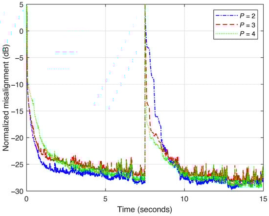
Figure 1. Normalized misalignment of the VR-RLS-TOT algorithm using different values of the decomposition parameter P. The forgetting factors ${\lambda }_{★}$, with $★\in \left\{2,12,11\right\}$, are set according to (52), using $K=30$. The input signal is a speech sequence, and the echo path changes after 7.5 s.

The advantage of the TOT-based decomposition lies in using a much smaller parameter space (i.e., a much smaller number of coefficients) compared to the conventional approach, which involves a single filter of length L. This is supported in Figure 2, where the filter indicated by “0” on the x-axis stands for the regular solution using $L=512$ coefficients. Here, the filters indicated as “1”, “2”, and “3” are associated with the TOT-based decomposition, with the lengths $L_2^2=4$ and $P{L}_{12}{L}_2=P{L}_{11}{L}_2=64$, which correspond to the current decomposition setup using $P=2$. Clearly, when using the TOT-based decomposition, there is an important reduction in terms of the parameter space, which further results in a lower computational complexity and an improved performance compared to the conventional approach.

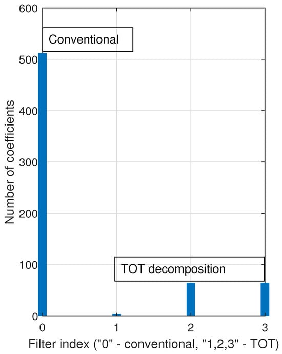
Figure 2. Parameter space (i.e., the number of coefficients) of the conventional approach ($L=512$) and the TOT-based decomposition, with $P=2$, $L_{11}=L_{12}=16$ and $L_2=2$ (i.e., $L_2^2=4$, $P{L}_{12}{L}_2=P{L}_{11}{L}_2=64$).

The forgetting factor is an important parameter that controls the performance of any exponentially weighted RLS-type filter. A larger value of the forgetting factor leads to a strong accuracy of the solution (i.e., low misalignment) but at the cost of a slow tracking behavior. On the other hand, reducing the value of this parameter affects the accuracy while improving the tracking capability. The proposed VR-RLS-TOT uses three forgetting factors, each one associated with one of the component filters. In Figure 3, their values are set using different values of the integer K, according to (52). This is the only parameter that has to be set for evaluating the values of ${\lambda }_{★}$ (with $★\in \left\{2,12,11\right\}$), since the lengths of the associated filters are known, i.e., $L_2^2$, $P{L}_{12}{L}_2$, and $P{L}_{11}{L}_2$, respectively. Clearly, the forgetting factors are always positive subunitary constants, as indicated by their role within the cost functions, i.e., to “forget” the past errors, so that the adaptive filter could be able to track the potential changes/variations in the system to be identified. As expected, a smaller value of K (i.e., a smaller forgetting factor) improves the tracking while also increasing the misalignment. For a better compromise in terms of these performance criteria, the “middle” value $K=30$ represents a favorable choice, which will be used in the following experiments for all the RLS-based algorithms. Of course, other values of K could be used, taking into account the previously discussed performance compromise.

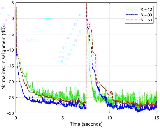
Figure 3. Normalized misalignment of the VR-RLS-TOT algorithm using different values of K for evaluating the forgetting factors ${\lambda }_{★}$, with $★\in \left\{2,12,11\right\}$, according to (52). The decomposition parameter is set to $P=2$. The input signal is a speech sequence and the echo path changes after 7.5 s.

Next, the proposed VR-RLS-TOT algorithm is compared to its TOT-based counterparts from [21,40], i.e., the RLS-TOT and R-RLS-TOT algorithms. Also, the VR-RLS algorithm from [31] is included in comparisons. The forgetting factors for all the algorithms are set using (52), with $K=30$. The decomposition parameter for the TOT-based algorithms is set to $P=2$, as outlined before. The results are presented in Figure 4. First, it can be noted that the proposed VR-RLS-TOT is more robust in terms of its accuracy, reaching a slightly lower misalignment level compared to the other two TOT-based algorithms, which are more affected by the nonstationary nature of the input signal (i.e., speech). Also, the VR-RLS-TOT algorithm exhibits strong tracking behavior when the echo path changes (after 7.5 s). In this case, we can notice a significantly slower reaction of the VR-RLS algorithm, which operates with a single (long-length) adaptive filter, with $L=512$ coefficients. On the other hand, the TOT-based algorithms combine the estimates provided by three (much) shorter adaptive filters, with 4, 64, and 64 coefficients, respectively (as indicated in Figure 2), which lead to an improved tracking behavior.

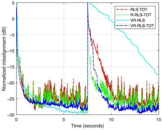
Figure 4. Normalized misalignment of the RLS-TOT [21], R-RLS-TOT [40], VR-RLS [31], and proposed VR-RLS-TOT. All the algorithms use $K=30$ for evaluating their corresponding forgetting factors, according to (52), while the TOT-based algorithms use the decomposition parameter $P=2$. The input signal is a speech sequence and the echo path changes after 7.5 s.

In the following, the robustness features of the algorithms are tested in noisy conditions when the microphone signal at the near end captures different signals in addition to the echo signal and the background noise. First, in Figure 5, two bursts of white Gaussian noise (WGN) are considered, with $\mathrm{SNR}=10$ dB and 0 dB, respectively. It can be noted that the proposed VR-RLS-TOT is very robust to such perturbations, while the other algorithms are significantly affected. The R-RLS-TOT [40] performs slightly better compared to the RLS-TOT [21], while the VR-RLS algorithm [31] has a certain latency related to its reactions and transitions due to the long-length filter that needs to be updated.

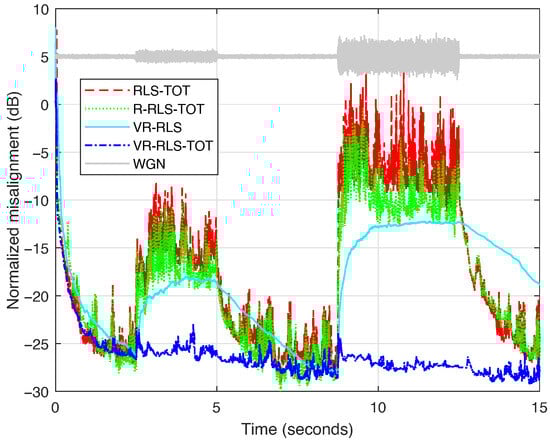
Figure 5. Normalized misalignment of the RLS-TOT [21], R-RLS-TOT [40], VR-RLS [31], and proposed VR-RLS-TOT. All the algorithms use $K=30$ for evaluating their corresponding forgetting factors, according to (52), while the TOT-based algorithms use the decomposition parameter $P=2$. The input signal is a speech sequence and two bursts of WGN are considered at the near end, with $\mathrm{SNR}=10$ dB and 0 dB.

Another scenario considers more challenging types of noise compared to the previous WGN bursts (which are stationary sequences). In Figure 6, the perturbation source (and its nature) is changing by using two bursts of highway noise and engine noise, respectively, while the latter is stronger. All the algorithms are more affected under these conditions compared to the previous WGN scenario. Nevertheless, the proposed VR-RLS-TOT still excels in terms of its robustness, being less affected by the first burst of highway noise while recovering fairly well in the case of the second burst of engine noise.

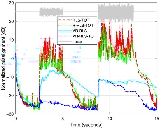
Figure 6. Normalized misalignment of the RLS-TOT [21], R-RLS-TOT [40], VR-RLS [31], and proposed VR-RLS-TOT. All the algorithms use $K=30$ for evaluating their corresponding forgetting factors, according to (52), while the TOT-based algorithms use the decomposition parameter $P=2$. The input signal is a speech sequence, and two bursts of different noises are considered at the near end, i.e., a highway noise and an engine noise, respectively.

Finally, the most challenging echo cancelation scenario is considered, which is the so-called double-talk case, when both speakers (far-end and near-end) talk at the same time [4]. In this scenario, the near-end speech acts like a large level of nonstationary disturbance for the adaptive filter. In Figure 7, two periods of double-talk appear, with different intensities, the second one being more significant. As we can notice, the behavior of both the RLS-TOT [21] and R-RLS-TOT [40] is seriously biased during double-talk. The VR-RLS algorithm [31] has some robustness in this scenario, but it is still influenced by the inherent latency due to operating with a long-length filter ($L=512$). On the other hand, the proposed VR-RLS-TOT algorithm quickly recovers at the beginning of the first period of double-talk while being very robust during the second period of (stronger) double-talk. Concluding, it achieves a much better compromise in terms of the main performance criteria compared to the competitive algorithms.

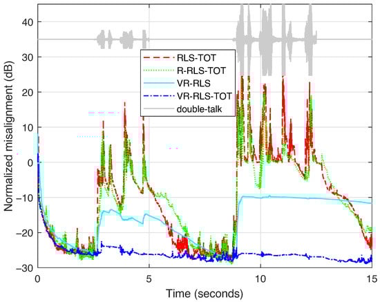
Figure 7. Normalized misalignment of the RLS-TOT [21], R-RLS-TOT [40], VR-RLS [31], and proposed VR-RLS-TOT. All the algorithms use $K=30$ for evaluating their corresponding forgetting factors, according to (52), while the TOT-based algorithms use the decomposition parameter $P=2$. The input signal is a speech sequence, and a double-talk scenario is considered, using two periods of near-end speech with different intensities.

5. Discussion

The proposed VR-RLS-TOT algorithm inherits the advantages of the tensor-based decomposition method and the robustness of a new regularization technique. As a result, its main strengths are related to a faster tracking capability and a better accuracy of the estimate, as compared to the conventional RLS-based algorithms, which do not involve the decomposition-based approach. Furthermore, since it operates with shorter adaptive filters (compared to the length of the global impulse response), the computational complexity of the proposed algorithm is also lower compared to its conventional RLS-type counterparts. In addition, the regularization method that incorporates the influence of external noise and model uncertainties provides additional robustness features, especially in noisy environments and nonstationary conditions. Thus, the VR-RLS-TOT algorithm could be a potential candidate for real-world scenarios and especially for real-time applications.

On the other hand, the fact that the proposed algorithm operates (in parallel) with three adaptive filters could raise some potential limitations. These component filters have different lengths and use different control parameters (i.e., forgetting factors and regularization terms). Hence, a synergy issue could arise, which should be addressed and evaluated by performing a detailed convergence analysis of the proposed algorithm. However, this is not a straightforward task and represents a self-contained objective, which will be addressed in future works.

There are several potential extensions of the proposed method, especially in conjunction with tensor-based signal processing techniques. In this context, interesting and useful connections could be established with neural network architectures and deep learning frameworks [41], where specific limitations are related to weakly supervised scenarios and noisy training situations.

6. Conclusions and Perspectives

This article has developed an RLS-type algorithm that exploits a TOT-based decomposition technique and operates with variable regularization parameters. The decomposition of the global impulse response using the TOT-based method leads to a combination of three shorter adaptive filters, with their coefficients connected using the Kronecker product. As a result, the parameter space of the conventional approach is significantly reduced, further leading to improved convergence and tracking while also achieving a lower computational complexity. Moreover, the variable regularization parameters associated with the three component filters are designed for improved robustness, especially in challenging conditions, e.g., when using nonstationary inputs and/or operating in noisy environments. The proposed VR-RLS-TOT algorithm has been tested in the framework of an echo cancelation scenario, under various (realistic) conditions, e.g., using speech as input, different types of noise, and double-talk. The obtained results have indicated the reliable performance of this algorithm, with a fast convergence rate and tracking, high accuracy, and robust behavior. Furthermore, it outperforms the previously developed TOT-based counterparts from [21,40], and also the conventional version of the RLS algorithm that uses the recently developed variable regularization technique [31].

Future work will focus on several main directions. First, we aim to develop computationally efficient versions of the VR-RLS-TOT algorithm, which exploit the line search methods [34,36] for solving the normal equations associated with the component filters. Second, a higher decomposition order will be investigated, targeting an improved factorization of the impulse response. Third, a comparative analysis with the family of Kalman filters will be conducted in the framework of tensor-based processing techniques. Finally, a detailed convergence analysis of the proposed algorithm will be considered. In this context, the main challenge is related to the connection between the three component filters, which also operate with different control parameters.

References

- Sayed, A.H. Adaptive Filters; Wiley: New York, NY, USA, 2008. [Google Scholar]
- Haykin, S. Adaptive Filter Theory, 5th ed.; Pearson: Upper Saddle River, NJ, USA, 2014. [Google Scholar]
- Diniz, P.S.R. Adaptive Filtering: Algorithms and Practical Implementation, 5th ed.; Springer Nature: Cham, Switzerland, 2020. [Google Scholar]
- Hänsler, E.; Schmidt, G. Acoustic Echo and Noise Control—A Practical Approach; Wiley: Hoboken, NJ, USA, 2004. [Google Scholar]
- Apolinário, J.A., Jr. (Ed.) QRD-RLS Adaptive Filtering; Springer: New York, NJ, USA, 2009. [Google Scholar]
- Rupp, M.; Schwarz, S. A tensor LMS algorithm. In Proceedings of the IEEE International Conference on Acoustics, Speech, and Signal Processing (ICASSP), South Brisbane, QLD, Australia, 19–24 April 2015; pp. 3347–3351. [Google Scholar]
- Rupp, M.; Schwarz, S. Gradient-based approaches to learn tensor products. In Proceedings of the European Signal Processing Conference (EUSIPCO), Nice, France, 31 August–4 September 2015; pp. 2486–2490. [Google Scholar]
- Ribeiro, L.N.; de Almeida, A.L.F.; Mota, J.C.M. Identification of separable systems using trilinear filtering. In Proceedings of the IEEE International Workshop on Computational Advances in Multi-Sensor Adaptive Processing (CAMSAP), Cancun, Mexico, 13–16 December 2015; pp. 189–192. [Google Scholar]
- Sidiropoulos, N.; Lathauwer, L.D.; Fu, X.; Huang, K.; Papalexakis, E.; Faloutsos, C. Tensor decomposition for signal processing and machine learning. IEEE Trans. Signal Process. 2017, 65, 3551–3582. [Google Scholar] [CrossRef]
- Ribeiro, L.N.; Schwarz, S.; Rupp, M.; de Almeida, A.L.F.; Mota, J.C.M. A low-complexity equalizer for massive MIMO systems based on array separability. In Proceedings of the European Signal Processing Conference (EUSIPCO), Kos, Greece, 28 August–2 September 2017; pp. 2522–2526. [Google Scholar]
- da Costa, M.N.; Favier, G.; Romano, J.M.T. Tensor modelling of MIMO communication systems with performance analysis and Kronecker receivers. Signal Process. 2018, 145, 304–316. [Google Scholar] [CrossRef]
- Ribeiro, L.N.; de Almeida, A.L.F.; Mota, J.C.M. Separable linearly constrained minimum variance beamformers. Signal Process. 2019, 158, 15–25. [Google Scholar] [CrossRef]
- Paleologu, C.; Benesty, J.; Ciochină, S. Linear system identification based on a Kronecker product decomposition. IEEE/ACM Trans. Audio Speech Lang. Process. 2018, 26, 1793–1808. [Google Scholar] [CrossRef]
- Elisei-Iliescu, C.; Paleologu, C.; Benesty, J.; Stanciu, C.; Anghel, C.; Ciochină, S. Recursive least-squares algorithms for the identification of low-rank systems. IEEE/ACM Trans. Audio Speech Lang. Process. 2019, 27, 903–918. [Google Scholar] [CrossRef]
- Bhattacharjee, S.S.; George, N.V. Nearest Kronecker product decomposition based normalized least mean square algorithm. In Proceedings of the IEEE International Conference on Acoustics, Speech, and Signal Processing (ICASSP), Barcelona, Spain, 4–8 May 2020; pp. 476–480. [Google Scholar]
- Bhattacharjee, S.S.; George, N.V. Fast and efficient acoustic feedback cancellation based on low rank approximation. Signal Process. 2021, 182, 107984. [Google Scholar] [CrossRef]
- Bhattacharjee, S.S.; George, N.V. Nearest Kronecker product decomposition based linear-in-the-parameters nonlinear filters. IEEE/ACM Trans. Audio Speech Lang. Process. 2021, 29, 2111–2122. [Google Scholar] [CrossRef]
- Bhattacharjee, S.S.; Patel, V.; George, N.V. Nonlinear spline adaptive filters based on a low rank approximation. Signal Process. 2022, 201, 108726. [Google Scholar] [CrossRef]
- Vadhvana, S.; Yadav, S.K.; Bhattacharjee, S.S.; George, N.V. An improved constrained LMS algorithm for fast adaptive beamforming based on a low rank approximation. IEEE Trans. Circuits Syst. II Express Briefs 2022, 69, 3605–3609. [Google Scholar] [CrossRef]
- Benesty, J.; Paleologu, C.; Ciochină, S. Linear system identification based on a third-order tensor decomposition. IEEE Signal Process. Lett. 2023, 30, 503–507. [Google Scholar] [CrossRef]
- Paleologu, C.; Benesty, J.; Stanciu, C.L.; Jensen, J.R.; Christensen, M.G.; Ciochină, S. Recursive least-squares algorithm based on a third-order tensor decomposition for low-rank system identification. Signal Process. 2023, 213, 109216. [Google Scholar] [CrossRef]
- Kolda, T.G.; Bader, B.W. Tensor decompositions and applications. SIAM Rev. 2009, 51, 455–500. [Google Scholar] [CrossRef]
- Comon, P. Tensors: A brief introduction. IEEE Signal Process. Mag. 2014, 31, 44–53. [Google Scholar] [CrossRef]
- Cichocki, A.; Mandic, D.P.; Phan, A.; Caiafa, C.F.; Zhou, G.; Zhao, Q.; Lathauwer, L.D. Tensor decompositions for signal processing applications: From two-way to multiway component analysis. IEEE Signal Process. Mag. 2015, 32, 145–163. [Google Scholar] [CrossRef]
- Zhou, N.; Trudnowski, D.J.; Pierre, J.W.; Mittelstadt, W.A. Electromechanical mode online estimation using regularized robust RLS methods. IEEE Trans. Power Syst. 2008, 23, 1670–1680. [Google Scholar] [CrossRef]
- Iqbal, N.; Zerguine, A. AFD-DFE using constraint-based RLS and phase noise compensation for uplink SC-FDMA. IEEE Trans. Veh. Technol. 2017, 66, 4435–4443. [Google Scholar] [CrossRef]
- Yang, F.; Yang, J.; Albu, F. An alternative solution to the dynamically regularized RLS algorithm. In Proceedings of the Asia-Pacific Signal and Information Processing Association Annual Summit and Conference (APSIPA), Lanzhou, China, 18–21 November 2019; pp. 1072–1075. [Google Scholar]
- Lawal, A.; Abed-Meraim, K.; Mayyala, Q.; Iqbal, N.; Zerguine, A. Blind adaptive channel estimation using structure subspace tracking. In Proceedings of the 55th Asilomar Conference on Signals, Systems, and Computers, Pacific Grove, CA, USA, 31 October–3 November 2021; pp. 1372–1376. [Google Scholar]
- Li, B.; Wu, S.; Tripp, E.E.; Pezeshki, A.; Tarokh, V. Recursive least squares with minimax concave penalty regularization for adaptive system identification. IEEE Access 2024, 12, 66993–67004. [Google Scholar] [CrossRef]
- Zhong, Y.; Yu, C.; Xiang, X.; Lian, L. Proximal policy-optimized regularized least squares algorithm for noise-resilient motion prediction of UMVs. IEEE J. Ocean. Eng. 2024, 49, 1397–1410. [Google Scholar] [CrossRef]
- Otopeleanu, R.A.; Benesty, J.; Paleologu, C.; Stanciu, C.L.; Dogariu, L.M.; Ciochină, S. A practical regularized recursive least-squares algorithm for robust system identification. In Proceedings of the European Signal Processing Conference (EUSIPCO), Palermo, Italy, 8–12 September 2025; pp. 1417–1421. [Google Scholar]
- Loan, C.F.V. The ubiquitous Kronecker product. J. Comput. Appl. Math. 2000, 123, 85–100. [Google Scholar] [CrossRef]
- Zakharov, Y.V.; Tozer, T.C. Multiplication-free iterative algorithm for LS problem. IEE Electron. Lett. 2004, 40, 567–569. [Google Scholar] [CrossRef]
- Zakharov, Y.V.; White, G.P.; Liu, J. Low-complexity RLS algorithms using dichotomous coordinate descent iterations. IEEE Trans. Signal Process. 2008, 56, 3150–3161. [Google Scholar] [CrossRef]
- Liu, J.; Zakharov, Y.V.; Weaver, B. Architecture and FPGA design of dichotomous coordinate descent algorithms. IEEE Trans. Circuits Syst. I Regul. Pap. 2009, 56, 2425–2438. [Google Scholar]
- Zakharov, Y.V.; Nascimento, V.H. DCD-RLS adaptive filters with penalties for sparse identification. IEEE Trans. Signal Process. 2013, 61, 3198–3213. [Google Scholar] [CrossRef]
- Claser, R.; Nascimento, V.H.; Zakharov, Y.V. A low-complexity RLS-DCD algorithm for Volterra system identification. In Proceedings of the European Signal Processing Conference (EUSIPCO), Budapest, Hungary, 29 August–2 September 2016; pp. 6–10. [Google Scholar]
- Bertsekas, D.P. Nonlinear Programming, 2nd ed.; Athena Scientific: Belmont, MA, USA, 1999. [Google Scholar]
- Digital Network Echo Cancellers. ITU-T Recommendations G.168. 2015. Available online: https://www.itu.int/rec/T-REC-G.168 (accessed on 14 November 2025).
- Otopeleanu, R.; Elisei-Iliescu, C.; Paleologu, C.; Benesty, J.; Ciochină, S. Regularized RLS algorithm based on third-order tensor decomposition. In Proceedings of the IEEE Conf. Advanced Topics Measurement Simulation (ATOMS), Constanta, Romania, 28–30 August 2024; pp. 307–310. [Google Scholar]
- Lee, K.; Lee, C.H. Weakly supervised graph neural network for line spectrum extraction. IET Radar Sonar Navig. 2025, 19, e70084. [Google Scholar] [CrossRef]
Disclaimer/Publisher’s Note: The statements, opinions and data contained in all publications are solely those of the individual author(s) and contributor(s) and not of MDPI and/or the editor(s). MDPI and/or the editor(s) disclaim responsibility for any injury to people or property resulting from any ideas, methods, instructions or products referred to in the content. |
© 2025 by the authors. Licensee MDPI, Basel, Switzerland. This article is an open access article distributed under the terms and conditions of the Creative Commons Attribution (CC BY) license (https://creativecommons.org/licenses/by/4.0/).