A Multi-Objective Evolutionary Computation Approach for Improving Neural Network-Based Surrogate Models in Structural Engineering

Abstract

Surrogate models are widely used in science and engineering to approximate other methods that are usually computationally expensive. Here, artificial neural networks (ANNs) are employed as surrogate regression models to approximate the finite element method in the problem of structural analysis of steel frames. The focus is on a multi-objective neural architecture search (NAS) that minimizes the training time and maximizes the surrogate accuracy. To this end, several configurations of the non-dominated sorting genetic algorithm (NSGA-II) are tested versus random search. The robustness of the methodology is demonstrated by the statistical significance of the hypervolume indicator. Non-dominated solutions (consisting of the set of best designs in terms of accuracy for each training time or in terms of training time for each accuracy) reveal the importance of multi-objective hyperparameter tuning in the performance of ANNs as regression surrogates. Non-evident optimal values were attained for the number of hidden layers, the number of nodes per layer, the batch size, and alpha parameter of the Leaky ReLU transfer function. These results are useful for comparing with state-of-the-art ANN regression surrogates recently attained in the recent structural engineering literature. This approach facilitates the selection of models that achieve the optimal balance between training speed and predictive accuracy, according to the specific requirements of the application.

1. Introduction

Solving real-world problems through computational engineering often requires a high computational time, even with increasingly efficient computers. Among the methods to reduce computational time and/or the number of evaluations of the objective function for improving optimal design in engineering using metaheuristics/evolutionary algorithms, we can fundamentally list the use of parallel evolutionary algorithms, the use of surrogate models or metamodels, and the use of game theory-based evolutionary algorithms [1]. This manuscript focuses on the second of these methods: efficient surrogate modeling is handled, particularly in the context of structural engineering and regression surrogate modeling, through artificial neural networks.

The application of neural networks in the calculation and optimization of skeletal structures is a field that was started some thirty years ago, as can be seen in references [2,3,4]. However, the recent surge in deep learning [5] and surrogate-based evolutionary algorithms [6] has recently fostered the research for enhancing single and multi-objective optimization [7] in real-world applications through surrogate-based evolutionary algorithms in many engineering fields, such as biomedical engineering [8], reliability engineering [9], and others [10]. In the field of structural engineering, ref. [11] proposes a single neural network architecture based on iterative tuning for the construction of a surrogate model. However, it does not provide details on the number of trials performed. In this case, the model is applied to the problem of reinforced concrete rigid node bar structures and had a six-layer hidden architecture with 128 neurons in the first two layers and 64 neurons in the last four layers. In ref. [12,13], surrogate models based on neural networks are proposed for an offshore wind turbine metal support bar structure. In the first case [12], 28 neural network architectures are tested, with possible combinations of one to four hidden layers and a uniform number of neurons per hidden layer of 10, 25, 50, 75, 100, 125 and 150. In the second case [13], only seven neural network architectures are tested consisting of 2, 3, 4, 5, 6, 7, 8 hidden layers and 100, 150, 200, 250, 300, 350, 400 neurons per layer, respectively. Whether detailing and proposing a single architecture or proposing even a limited set of architectures for the neural network-based surrogate model, there is scope to improve the performance of the surrogate if an optimization procedure is handled to improve the architecture and/or hyperparameters of the neural network.

The enhancement of the neural network architecture and parameters has been handled through the procedure known as Neural Architecture Search (NAS) [14,15]. The most commonly used algorithms for NAS are reinforcement learning, Bayesian optimization, and evolutionary algorithms/metaheuristics, with the latter being employed successfully in multi-objective optimization approaches. In single-objective NAS, where the minimization of error (or alternatively the maximization of accuracy) is typically sought, the complexity of the neural network (or the computational training time required) is not a factor that is taken into consideration. Conversely, within the paradigm of multi-objective optimization, a secondary objective function is incorporated, namely training time, as elucidated in this study. This enables the identification of a set of non-dominated solutions, signifying the attainment of the ANN architecture that corresponds to the optimal accuracy for a specific training time. Alternatively, this approach facilitates the identification of the ANN architecture that attains the lowest training time for a given level of accuracy. The extant literature on the use of neural networks as surrogate models/metamodels in structural engineering has recently been augmented with the incorporation of four recent reviews, which are indicative of the growing interest in this field of research [16,17,18,19]. It is evident from the research undertaken to the best of the authors’ knowledge that this work is pioneering in its proposal, implementation, and successful demonstration of a multi-objective NAS in the field of structural engineering. A comprehensive survey of the literature reveals no previous suggestion or successful application of a multi-objective NAS in this area. The conflicting objectives are commonly related to the accuracy of the surrogate model accuracy and the efficiency of the hardware [20,21], although the complexity of the neural network is also considered (the number of parameters is frequently taken into account). In this manuscript, the conflicting objectives are related to improving first, surrogate model accuracy and second, surrogate model calculation speed.

This work focuses on enhancing efficient neural network-based surrogate models. A multi-objective approach using evolutionary algorithms is proposed for the improvement of surrogate models in bar element structures. This approach aims to produce models that are as accurate as possible (being able to faithfully reproduce the associated numerical method) and simultaneously as fast as possible (training/calculation time of the surrogate model as short as possible). To this end, this work employs a state-of-the-art multi-objective evolutionary algorithm based on the Pareto dominance criterion (the non-dominated sorting genetic algorithm NSGA-II [22]) and a surrogate deep learning model using artificial neural networks. The field of multi-objective optimization is still an active research field (e.g., some recent multi-objective algorithms are proposed in [23,24]). As example, the PlatEMO framework [25] available in (https://github.com/BIMK/PlatEMO, accessed on 31 October 2025), currently has (release 4.13) more than 300 multi-objective evolutionary algorithms. For this research, the state-of-the art multi-objective evolutionary algorithm NSGA-II was chosen because it is the most used and cited algorithm and still a state-of-the-art approach for solving optimization problems with two objectives [26], as it is the handled problem.

From a database of thousands of structures, the results successfully demonstrate the application of the methodology in a reference test case from the scientific literature of frame steel structures [27]. They provide a set of non-dominated solutions with optimal accuracy and computational time, as well as useful insights about the hyperparameters of the neural network-based surrogate model.

The structure of the manuscript continues as follows: Section 2 presents the structural problem and test case. Section 3 then introduces the multi-objective optimization NAS approach, as well as the structure and configuration of the neural networks used. Section 4 presents the experimental results and discussion. Finally, Section 5 presents the conclusions.

2. Structural Engineering Problem and Test Case

The goal of the structural problem addressed is an optimal design problem where we want to obtain the lowest weight (equivalently mass) structure, which in turn can fulfill the mission for which it was designed. This mission consists of resisting the loads to which it is subjected without reaching the ultimate and serviceability limit states; that is, without exceeding the maximum constraints related to the limit stresses of the material and the limit deformations, both established in the regulations.

Usually, these evaluations of stress and displacements are carried out using a finite element method, which will be described in Section 2.1. Some considerations about skeletal frame structures are shown in Section 2.2. Finally, the handled test case is described in Section 2.3.

2.1. Finite Element Method

Structural calculation involves solving a finite element model (FEM) [28] with Hermite approximation functions and its associated system of linear equations.

In the flat case (as is the test case to be solved) each node has three degrees of freedom in displacement: horizontal, vertical, and rotation, in addition to three types of associated force: horizontal force, vertical force, and moment. The vectors of forces (F) and displacements (U) are related through the stiffness matrix (K): F = KU. This matrix K depends on the geometrical properties of the section and the material properties and is created by an assembly process from each element (member) of the structure. To reduce the bandwidth of the matrix and consequently its calculation time, the inverse Cuthill–McKee renumbering method is applied, after which the system of equations is solved, obtaining the displacements of the nodes. From these, the stresses in any section of the structure can be calculated.

The next step is to obtain, by applying the direct method of stiffness described above, from the definition of the design variables of a skeletal structure (positions of the nodes, connectivity of the members, geometry of the section of each member, loads to which it is subjected, links, material), the weight/mass, and the values of stresses and displacements.

Finally, after calculating the stresses and displacements with FEM, they are compared with the limit values established for stresses (for each bar) and displacements (for certain specified nodes). If any of these are exceeded, their value is added to the violation of the global constraint, which is the value to be predicted by the surrogate model.

2.2. Skeletal Frame Structures

The geometrical properties of the cross-section that influence the calculation of stresses and strains explained in the previous section depend on the type of structure considered.

In the case of structures with articulated nodes (trusses), they are characterized by having loads only at the nodes and not resisting moments, and only the cross-section area is required. In the case of member structures with rigid nodes (frames), as is the test case to be solved, where the nodes between the members are rigid and moments must be considered, more geometrical magnitudes of the member must be considered in the calculation. In addition to the area, other magnitudes such as the section modulus, the section height ratio, and the moment of inertia must be considered.

In the design of structures in the real world, standardized cross-sections are used and are included in databases [29] listed by cross-section shapes such as IPE in Europe or S in America (I-shaped sections), HEB in Europe, or W in America (H-shaped sections).

2.3. Test Case

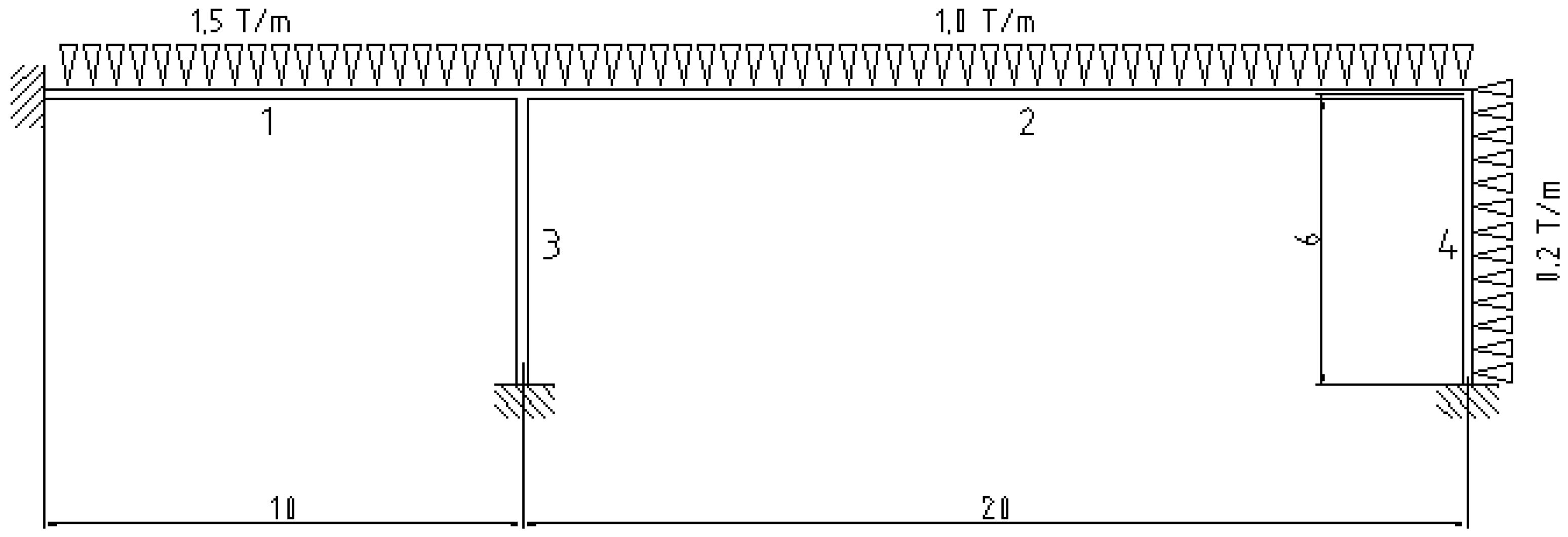
The test case handled in this article is based on the one published in [30], which deals with the optimization of continuous sections. This test case is utilized as a reference test case in the optimization of steel structures with rigid nodes by means of evolutionary algorithms from [27], considering normalized cross-sections (discrete variables), as useful in the real engineering case. It is a four-bar structure subjected to loads and geometry (dimensions in meters), as described in Figure 1.

Figure 1. Test case. Frame structure dimensions and loads (lengths in meters; loads in T/m).

The density and modulus of elasticity correspond to the values of standard structural steel as follows: 7850 kg/m³ and 2.1 × 10⁵ MPa, respectively. A maximum displacement at the midpoint of the longest beam (bar numbered 2 in Figure 1) of its length divided by 300 is also considered. All bars belonging to the IPE type, from IPE-080 to IPE-600 (eighteen types), with allowable stresses of 240 MPa, are considered.

All the data described above (design parameters) are necessary for the calculation of the structure as explained in previous subsections. In the case of the discrete sizing optimization problem, the design variables are exclusively the type of cross-section of each of the four members of the frame. These indices will be considered as input data of the surrogate model, with the value of the constraints of the problem (stresses and displacements) being its output. The description of the surrogate model is presented in the following section.

3. Artificial Neural Network Surrogate Model and Neural Architecture Search

3.1. Mathematical Description

In this section, the definition of the multi-objective optimization problem (Section 3.1) and the neural network (Section 3.2) were introduced.

3.1.1. Definition of the Multi-Objective Optimization Problem

The need to minimize objective functions F₁(x) and F₂(x) through the set of decision variables x(t) = {x₁, x₂, x₃, x₄}.

The multi-objective optimization problem consists of optimizing two objective functions simultaneously, which are conflicting:

min [F₁(x), F₂(x)], being F(x) the vector of objective functions,

where

-

F₁(x) is the training time of the artificial neural network model (in minutes)

-

F₂(x) is the lowest validation loss obtained during the training process

-

x₁ is the number of hidden layers

-

x₂ is the number of nodes per layer

-

x₃ is the batch size

-

x₄ is the alpha parameter of the Leaky ReLU activation function

The problem addressed in this work involves two objective functions to be minimized, without any constraints.

3.1.2. Neural Network

In this work a deep neural network of fully connected perceptrons is proposed, based on the following definitions: perceptron, neural network via forward propagation, Leaky ReLU activation function, and mean squared error loss function.

Perceptron: The perceptron is the basic mathematical model of an artificial neuron. Given an input vector x ∈ R^d, a weight vector w ∈ R^d, and a bias term b ∈ R^d, the perceptron computes:

z = w^T x + b

h = ϕ(z)

where ϕ(·) is the non-linear activation function (Leaky ReLU). The perceptron therefore applies a linear transformation followed by non-linearity.

Neural Network via Forward Propagation: Stacking multiple perceptrons arranged in layers can lead to the construction of a deep neural network. Let the network consist of L layers; the network input is defined as:

h(0) = x

For each layer l = 1, 2, …, L:

z(l) = W(l) h(l − 1) + b(l)

h(l) = ϕ(z(l))

where W(l) and b(l) are, respectively, the weights and the biases of layer l.

The final output of the network is:

ŷ = h(L)

This sequential computation contributes the forward pass.

Leaky ReLU Activation function: The Leaky ReLU activation function mitigates the “dying ReLU” problem by allowing a small, non-zero gradient for negative inputs. It is defined as:

$$\mathsf{\varphi }(\mathrm{z})=\left\{\begin{array}{c}z if z\ge 0\\ \alpha z if z<0\end{array}\text{ → being }\mathrm{\alpha }>0\right.$$

Its derivative, used during gradient-based optimization, is:

$$\mathsf{\varphi }’(\mathrm{z})=\left\{\begin{array}{c}1 if z\ge 0\\ \alpha if z<0\end{array}\right.$$

Loss Function: Mean Squared Error (MSE): Given a dataset {(x_i, y_i)} ∀i∈{1, …, n}, the output of the network for input x_i is ${\hat{\mathrm{y}}}_i$ = f(x_i; θ), where θ denotes all network parameters. The MSE loss is defined as:

$$L\left(\theta \right)={\displaystyle \frac{1}{n}}\sum _{i=1}^n{(y_i-{\hat{\mathrm{y}}}_i)}^2$$

Training the network consists of minimizing L(θ) with respect to the parameters θ = {W(l), b(l)}.

3.2. Methods: Multiobjective NAS in Structural Engineering

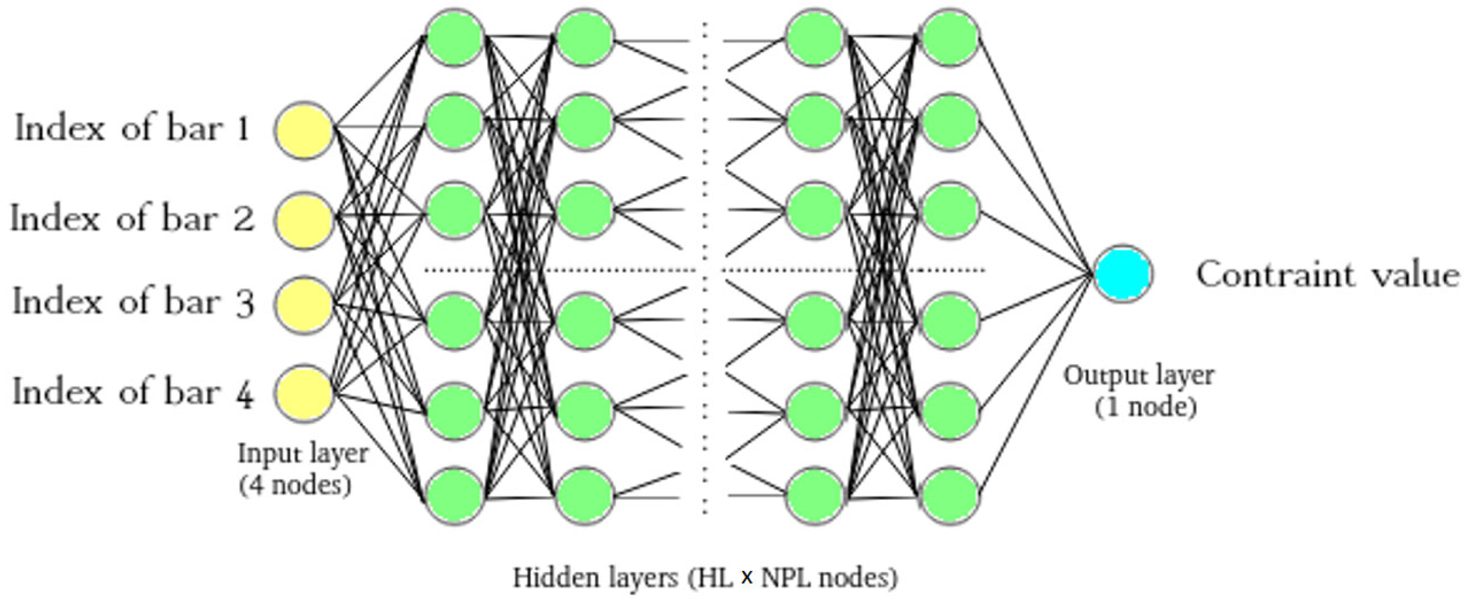
For the structural calculation surrogate models, fully connected ANNs are employed (Figure 2). These models take as input the structural cross-section types, each characterized by their cross-sectional area and moment of inertia, as specified in Table 1. The multilayer perceptron architecture has been selected on the basis of its prevalence in the extant literature, which has been reviewed in order to ascertain its use as a surrogate model for structural skeletal problems (for regression approximation of the finite element method of the structural constraints as stresses or displacements). It is acknowledged that alternative architectures are beginning to emerge (e.g., CNNs or graph-based models; see [18,19]); however, the multiobjective NAS approach introduced here for structural engineering could be tested in those other architectures in the future.

Figure 2. Structure of the fully connected artificial neural network in this work; input layer (yellow), hidden layers (green) and output layer (cyan); where HL: number of hidden layers; NPL: number of neurons per layer.

Table 1. Area and moment of inertia values of each IPE cross-section type.

Index	Profile	Area (cm2)	Moment of Inertia (cm4)
1	IPE080	7.6	80.14
2	IPE100	10.3	171
3	IPE120	13.2	318
4	IPE140	16.4	541
5	IPE160	20.1	869
6	IPE180	23.9	1320
7	IPE200	28.5	1940
8	IPE220	33.4	2770
9	IPE240	39.1	3890
10	IPE270	45.9	5790
11	IPE300	53.8	8360
12	IPE330	62.6	11,770
13	IPE360	72.7	16,270
14	IPE400	84.5	23,130
15	IPE450	98.8	33,740
16	IPE500	116	48,200
17	IPE550	134	67,120
18	IPE600	156	92,080

In this optimization problem, eighteen distinct cross-section types are considered, each represented by a numerical index ranging from 1 to 18. These indices are associated with the physical properties of the cross-section types—specifically, their area and moment of inertia. For the construction of each neural network model, the indices corresponding to the four structural cross-section types of the structure (see Figure 1) are considered as inputs.

This approach simplifies the original input—consisting of the geometrical properties per cross-section type—into a single integer value ranging from 1 to 18, reducing the number of network inputs and minimizing their range of values.

The neural network aims to predict the structural constraint value based on the input cross-section types of the structure. In this study, a dataset comprising 65,536 precomputed structures has been considered. The solved test case employed in this study is illustrated in Figure 1, while the architecture of the artificial neural network is demonstrated in Figure 2. In this context, the database contains 65,536 structures, comprising consecutive IPE120 to IPE600 (16 cross-section types) for bars 1, 2, and 4, and IPE080 to IPE500 (16 cross-section types) for bar 3, as defined in the optimization problem cited in [27]. To train, validate, and test the neural network models, this dataset is divided into separate subsets. Given the high computational cost associated with training each model and the large number of training processes required, two reduced training set sizes—5% and 15% of the full dataset—have been selected. For the validation and test phases, 10% of the dataset is consistently allocated to each, ensuring that the data in these subsets are entirely distinct from the training data and from each other. The assignment of data to the training, validation, and test sets is performed randomly and independently of the row order in the original dataset.

Each ANN model will use the ADAM optimizer [31] and the Leaky ReLU activation function [32] and will be trained over a total of 300 epochs. To generate the ANN models, an ADAM optimizer is used with its default settings. This means that the optimizer is configured to work without weight decay, gradient clipping, or moving average of weights; the parameters used in weight updating have the following values: α (learning rate) = 0.001; β₁ = 0.9; β₂ = 0.999; ε = 10⁻⁷. On the other hand, the loss function used is the mean squared error (MSE) in its simple form, without loss weighting or weights involved. No regularization method or dropout is being used either.

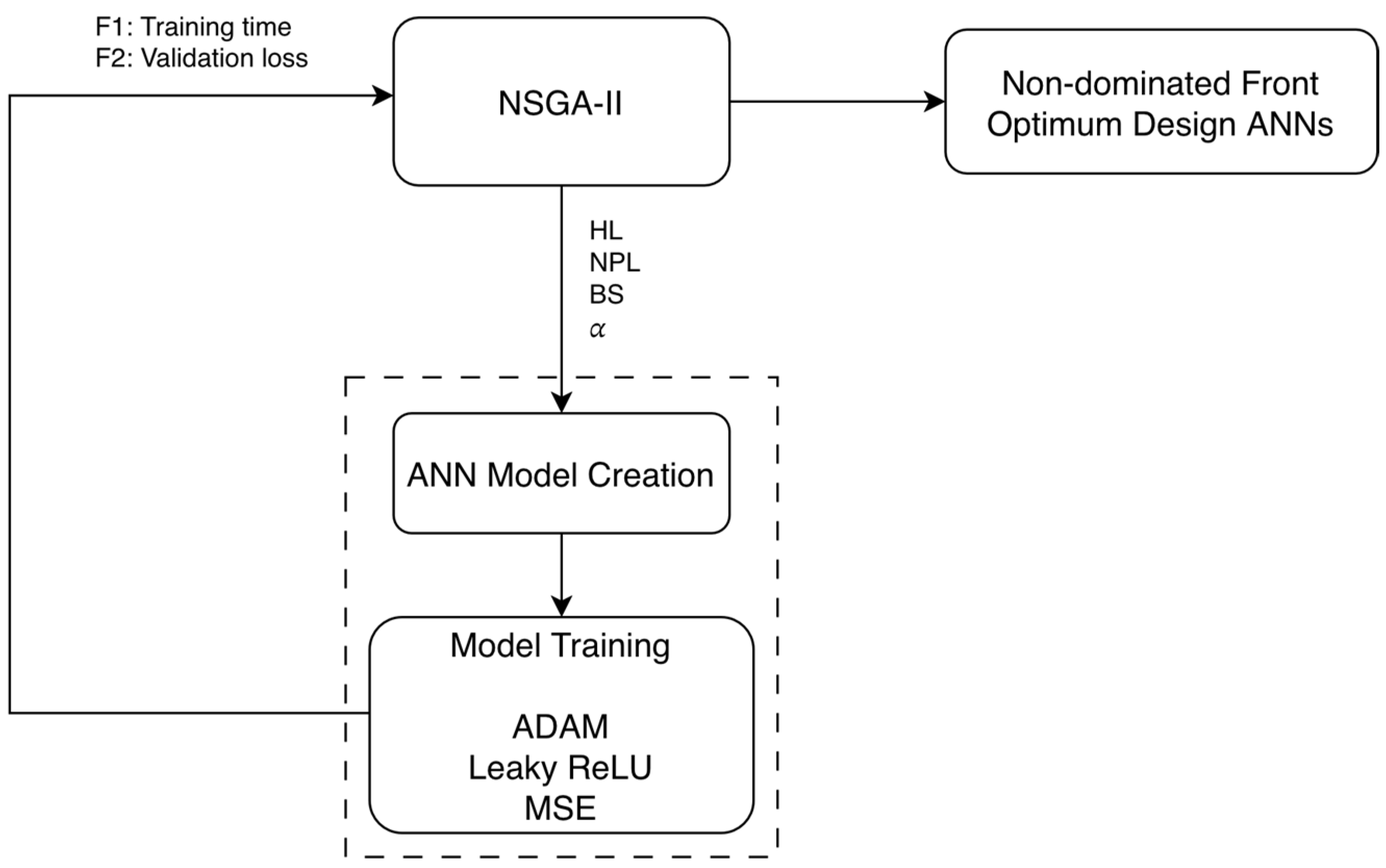
Consequently, the training process involves a significant computational cost, while the model’s accuracy is evaluated during the training using the validation loss. Through a multi-objective Neural Architecture Search (NAS), the final objective is to find a set of models capable of obtaining maximized models in terms of accuracy (i.e., the aim is to minimize the validation loss in terms of Mean Squared Error MSE) and minimize models in terms of training time. For this purpose, the NSGA-II algorithm is the multi-objective evolutionary optimization method. A flowchart of the general procedure is shown in Figure 3.

Figure 3. Flowchart of the algorithmic approach, where HL: number of hidden layers; NPL: number of neurons per layer; BS: batch size; α: alpha parameter of Leaky ReLU.

Two population sizes (24 and 30) were considered. Each individual (or chromosome) is represented by a set of four design variables (or genes), which are explained below, specifying their minimum and maximum values:

• Number of hidden layers: 1–7.
• Number of nodes or neurons, per hidden layer: 10–400.
• Batch size used for training: 32–1024.
• Alpha parameter of the Leaky ReLU activation function: 0.05–0.50.

The ranges of the hyperparameters are of the same order as those cited in the works referenced in the introduction. The findings indicate that the selected ranges facilitate the acquisition of a diverse range of model types within the non-dominated front.

Leaky ReLU is an activation function used in ANN. This function is a variant of the ReLU (Rectified Linear Unit) function, which is popularly used in neural networks. The Leaky ReLU function is similar to the ReLU function, but instead of having a zero slope for negative values, it has a small slope. This means that the function does not stop completely at negative values, which can help prevent neuron saturation.

NSGA-II uses a binary simulated crossover SBX (crossover rate is 90% and crossover index is 20%) and polynomial mutation (following the general rule of setting it as the inverse of the number of design variables, mutation rate is 25% and mutation index is 20%).

Four different experiments are considered: 24 and 30 population sizes, with and without scaling fitness functions, with a stopping criterion of 3000 fitness function evaluations. If the order of magnitude of the objective functions is highly different, the optimization procedure can be affected: the crowding operator of the selection operator of the NSGA-II algorithm is used to calculate the distances between adjacent individuals by adding the values of the objective functions; however, this could not be a fair comparison if the functions have very different magnitudes. To study this effect a scaled fitness function (training time divided by 30 and validation loss is divided by 2 × 10⁹) is used and compared to the non-scaled case in the experiments. Moreover, scaling is mandatory when computing the hypervolume (HV) indicator [33]. HV is a compliant quality indicator that represents the area formed by the non-dominated front of solutions of a population of individuals with respect to a reference point, which is set at [1.1, 1.1] for the problem discussed in this article. The calculation of the hypervolume is meaningless if the objective values exceed a predefined reference point [1.1, 1.1] in this work. To adjust the values of the non-scaled objective functions below the reference point exclusively for the HV calculation, the training time is divided by 30 and the validation loss by 2 × 10⁹.

Each experiment is executed taking into account nine independent cases. A total of 2 training set sizes (5% and 15%), times 2 population sizes (24 and 30), times 2 fitness function calculations (without and with scaling), times 9 independent executions reach a total of 2 × 2 × 2 × 9 = 72 runs of the evolutionary algorithm.

Mean and median convergence of HV curves, as well as Friedman statistical significance and post hoc tests, will be taken into account to measure the performance of the abovementioned experiments. They are also compared versus random search; these random individuals are trained independently, without an evolutionary process that allows for the selection, crossover, and mutation of the best ones.

The accumulated non-dominated fronts among the whole set of experiments will also be calculated, and those optimal artificial neural network designs from the multi-objective point of view will be trained using the 80% of the database as training set and a 10% as validation set, with the objective of observing the performance of the optimal models with the full available dataset. After a model is trained, it is tested using the remaining 10% of the available data (test set), whose accuracy is measured in terms of the MSE.

All experiments were implemented in Python 3.12.7 [34]. Multi-objective optimization was performed using the NSGA-II algorithm, as implemented in the pymoo 0.6.1.6 library [35], while neural network training was carried out using TensorFlow 2.17 [36]. These libraries constitute the core tools for the evolutionary search and model training processes. Friedman and post hoc statistical significance tests were performed using the software available in ref. [37].

Computational experiments were executed on a Linux-based cluster, with the workload manually distributed across five nodes. Each node was equipped with two Intel Xeon Silver 4314 processors (16 cores) and 128 GB of RAM. The experiments were executed on CPU cores that are exclusive. In the context of the experimental design, it is imperative to note that each experiment is subjected to nine parallel repetitions, encompassing four distinct configurations of the primary experiment. These configurations include population sizes of 24 and 30, with and without scaling, respectively. Additionally, two training set sizes are considered, namely 5% and 15%. Consequently, this results in 36 runs of the NSGA-II algorithm for each training size, with 3000 ANN trainings conducted in each execution. The time specified in this article is the average for each of the 36 executions: the first category, which was observed to last 7 days and 10 h (5%), and the second category, which was observed to last 10 days and 6 h (15%).

4. Experimental Results and Discussion

This section presents the experimental results obtained from the application of the NSGA-II algorithm to the multi-objective optimization of neural network surrogate models. The analysis focuses on the evolution of the hypervolume (HV) indicator, which reflects the quality of the non-dominated solutions in terms of training time and validation loss.

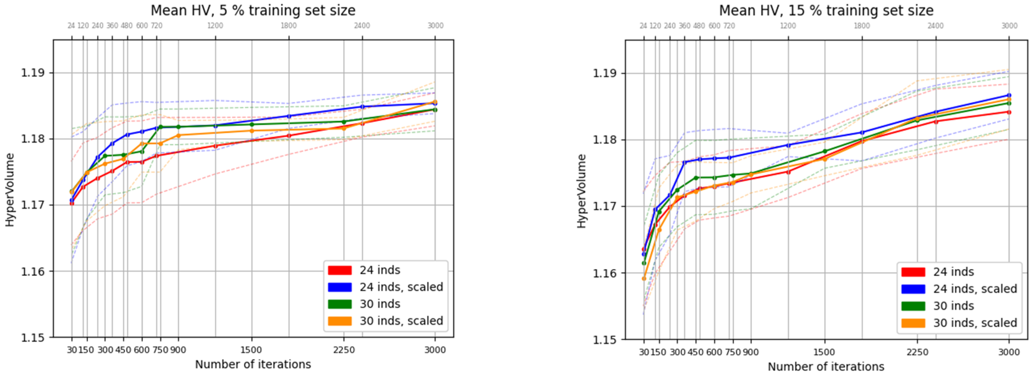
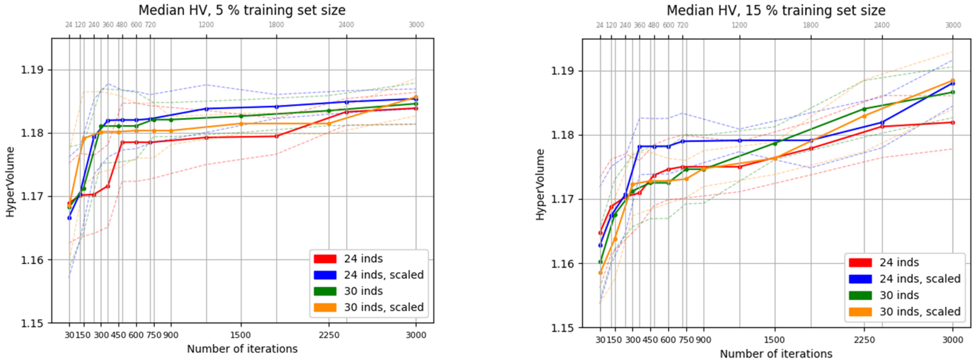
Figure 4 shows the evolution of the mean HV indicator across 9 independent runs of NSGA-II, using population sizes of 24 and 30, over 3000 fitness function evaluations. The experiments were conducted both with and without fitness function scaling. The left side of the figure corresponds to the case with a 5% training set size, while the right side shows results for a 15% training set size. The vertical scales are equivalent, allowing for a direct comparison between configurations.

Figure 4. Mean hypervolume convergence; training set sizes 5% (left) and 15% (right); dashed lines represent one standard deviation boundaries.

It can be observed that, with equivalent vertical scales, the initial hypervolume (HV) values in the 5% training set case—where training is faster—are slightly higher, ranging from 1.170 to 1.173, compared to the 15% case, which ranges from 1.158 to 1.165. However, after reaching the stopping criterion of the evolutionary process, the final HV values are superior in the 15% training set case, exceeding 1.185 in 3 out of 4 runs. This improvement is attributed to the larger training set, which enables the surrogate models to achieve greater accuracy.

A similar trend is observed in Figure 5, which shows the convergence of the median HV indicators. The final HV values in the scaled cases (represented by the blue and yellow lines) are consistently higher than those in the non-scaled cases. The configuration with the smallest population size (24 individuals and 125 generations) and no fitness scaling—represented by the red line—exhibits the lowest performance.

Figure 5. Median hypervolume convergence; training set sizes 5% (left) and 15% (right); dashed lines represent standard deviation boundaries.

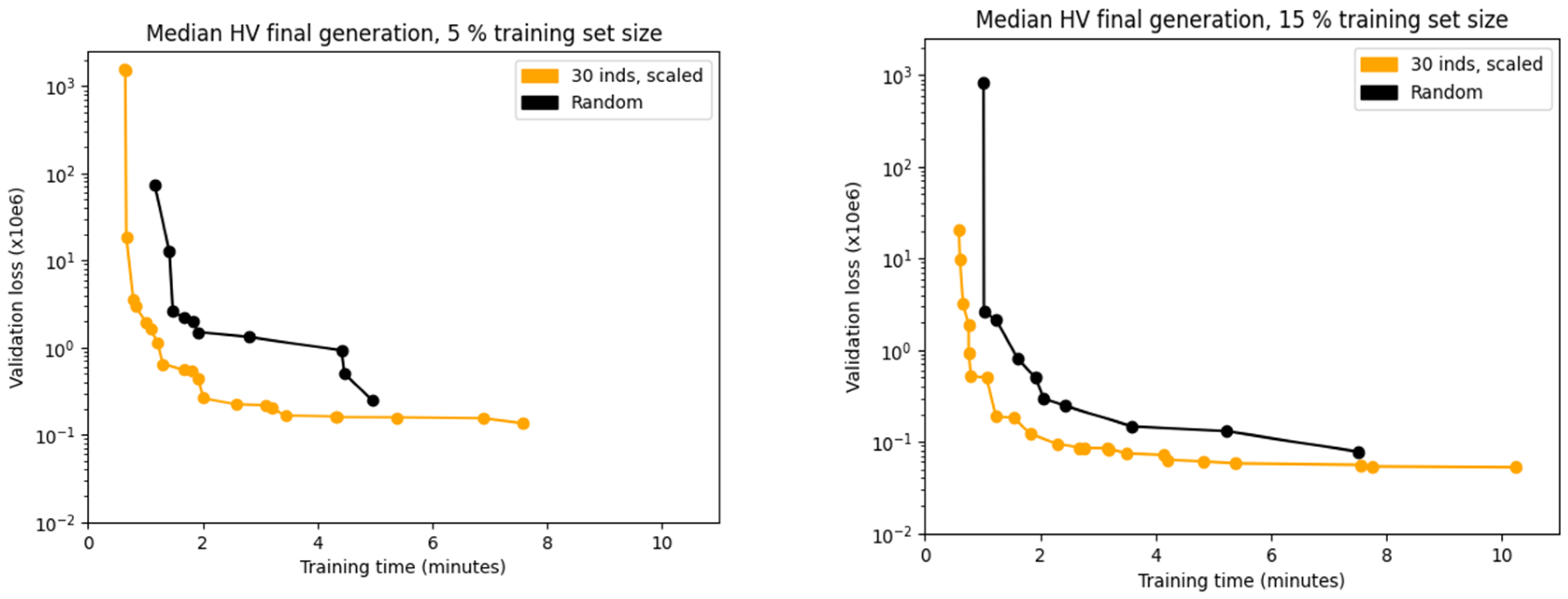
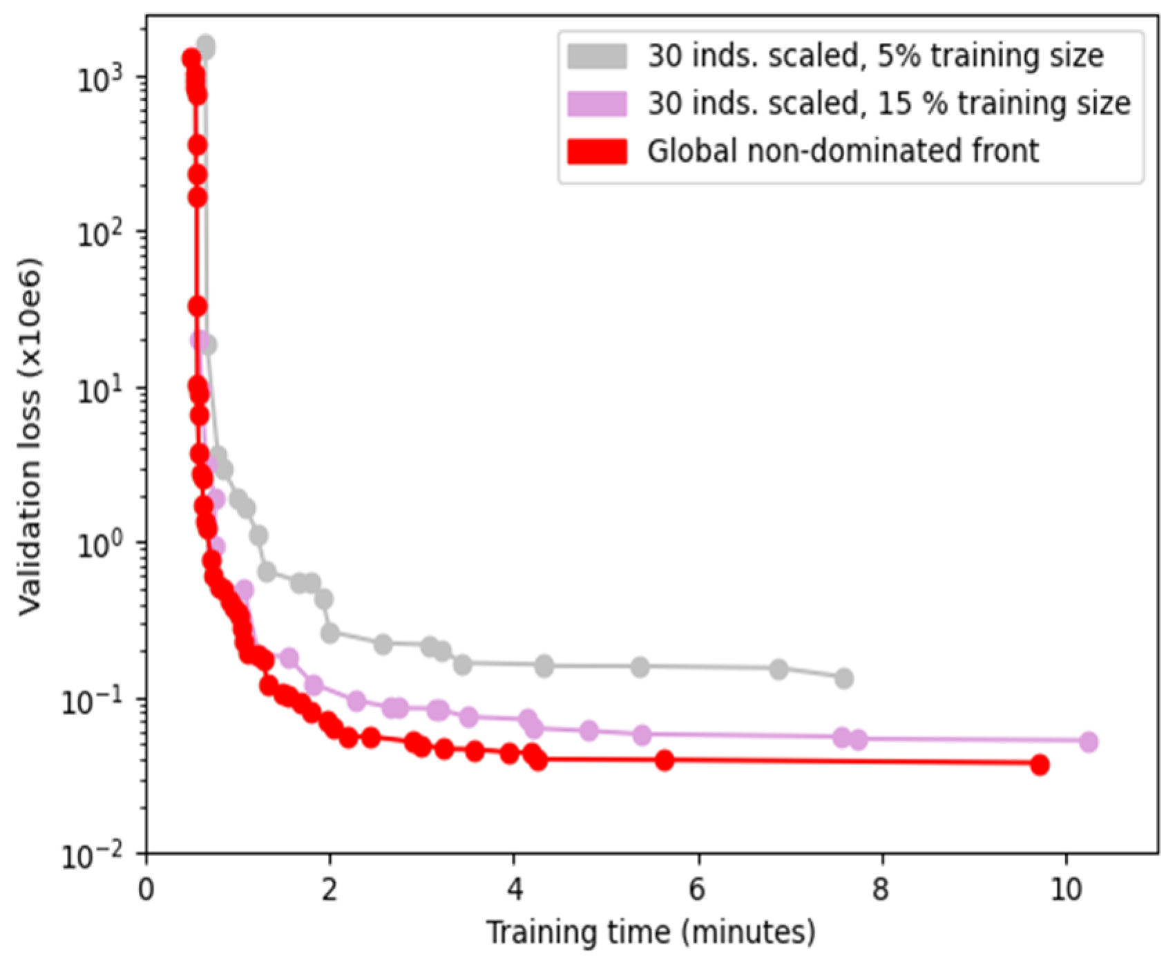
Median non-dominated fronts at stopping criterion of the case of 30 population size scaling fitness functions versus random search are shown in Figure 6. NSGA-II optimization designs clearly dominate the random search solutions (yellow curves are lower and more left than black curves) in both training set sizes. Median non-dominated front of the 15% training set size dominates the one of the 5% training set size, also clearly appreciated in pink and gray lines of Figure 7.

Figure 6. Median non-dominated front (based on HV value, 9 independent executions); population size 30, scaled fitness functions versus random. Training set sizes 5% (left) and 15% (right).

Figure 7. Global accumulated non-dominated front versus median fronts of 5% and 15% training sizes (as in Figure 5).

The convergence data from the optimisation processes carried out (both populations and hypervolume indicator values) are available as a Supplementary File associated with this manuscript.

The global accumulated non-dominated front obtained from all tested experiments, consisting of 49 neural network designs, is shown as a red line in Figure 7. Detailed information on these designs—including hyperparameter configurations, corresponding experimental settings, and fitness function values—is provided in Table 2, sorted from lowest to highest training time (and inversely, from highest to lowest validation loss). It can be observed that the accumulated front dominates the pink and gray fronts, which correspond to the yellow curves previously shown in Figure 6.

Table 2. Accumulated non-dominated solutions (5% + 15% training set sizes), including hyperparameters values.

Rank	Experiment	Training Set Size (%)	Hidden Layers	Nodes per Layer	Batch Size	Alpha	Training Time (Minutes)	Validation Loss (×106)
1	30_inds_scaled	15	1	21	1022	0.221	0.489	1315.09
2	24_inds	5	2	24	890	0.0832	0.526	1035.59
3	24_inds_scaled	15	2	11	929	0.0742	0.535	932.71
4	30_inds_scaled	5	3	14	707	0.0656	0.539	839.73
5	30_inds_scaled	5	3	14	697	0.0656	0.544	759.70
6	30_inds_scaled	15	2	17	669	0.0521	0.547	364.52
7	30_inds	5	3	40	996	0.0674	0.547	234.56
8	30_inds	15	3	18	975	0.067	0.558	168.74
9	30_inds_scaled	5	7	11	1012	0.0656	0.558	32.94
10	30_inds_scaled	15	5	14	1023	0.0583	0.564	10.25
11	30_inds	15	4	15	870	0.0691	0.568	9.03
12	30_inds_scaled	15	5	20	1022	0.218	0.568	6.54
13	24_inds_scaled	15	4	30	989	0.0958	0.578	3.76
14	30_inds_scaled	5	7	37	738	0.0678	0.604	2.76
15	30_inds	5	7	40	996	0.0674	0.614	2.59
16	30_inds_scaled	15	7	29	968	0.0747	0.627	1.73
17	30_inds_scaled	15	7	29	951	0.0733	0.641	1.37
18	30_inds	15	6	37	630	0.0667	0.660	1.22
19	30_inds	15	6	44	637	0.0671	0.715	0.783
20	30_inds	15	6	44	530	0.0741	0.727	0.614
21	30_inds_scaled	15	6	47	297	0.0555	0.798	0.512
22	24_inds	15	7	55	331	0.0634	0.853	0.505
23	30_inds	15	5	158	985	0.0559	0.917	0.415
24	30_inds	15	5	136	932	0.0514	0.946	0.381
25	30_inds	15	5	131	796	0.05613	0.991	0.354
26	30_inds	15	5	136	845	0.0508	1.01	0.335
27	30_inds_scaled	15	4	97	207	0.0599	1.04	0.285
28	30_inds_scaled	15	6	79	251	0.0663	1.06	0.228
29	24_inds	15	7	76	205	0.0728	1.12	0.191
30	30_inds_scaled	15	7	78	181	0.0701	1.23	0.189
31	24_inds	15	5	75	124	0.0720	1.28	0.176
32	30_inds_scaled	15	5	136	199	0.0513	1.32	0.123
33	30_inds_scaled	15	4	119	124	0.0525	1.50	0.107
34	24_inds	15	4	134	159	0.0546	1.55	0.102
35	30_inds_scaled	15	4	119	124	0.0523	1.68	0.0918
36	24_inds	15	3	259	174	0.0646	1.81	0.0820
37	24_inds	15	3	259	176	0.0646	1.98	0.0717
38	24_inds_scaled	15	3	294	154	0.0532	2.03	0.0646
39	24_inds_scaled	15	3	219	90	0.0558	2.20	0.0562
40	30_inds_scaled	15	3	204	71	0.0526	2.43	0.0560
41	24_inds_scaled	15	3	226	57	0.0532	2.90	0.0519
42	30_inds_scaled	15	3	335	94	0.0590	3.00	0.0497
43	30_inds_scaled	15	3	335	94	0.0590	3.23	0.0467
44	24_inds_scaled	15	3	286	56	0.0628	3.57	0.0463
45	30_inds_scaled	15	3	304	38	0.0852	3.95	0.0444
46	24_inds_scaled	15	3	288	41	0.0557	4.18	0.044
47	24_inds	15	3	373	69	0.0644	4.26	0.0400
48	24_inds	15	3	343	51	0.0633	5.62	0.0396
49	30_inds_scaled	15	3	304	38	0.0577	9.70	0.0379

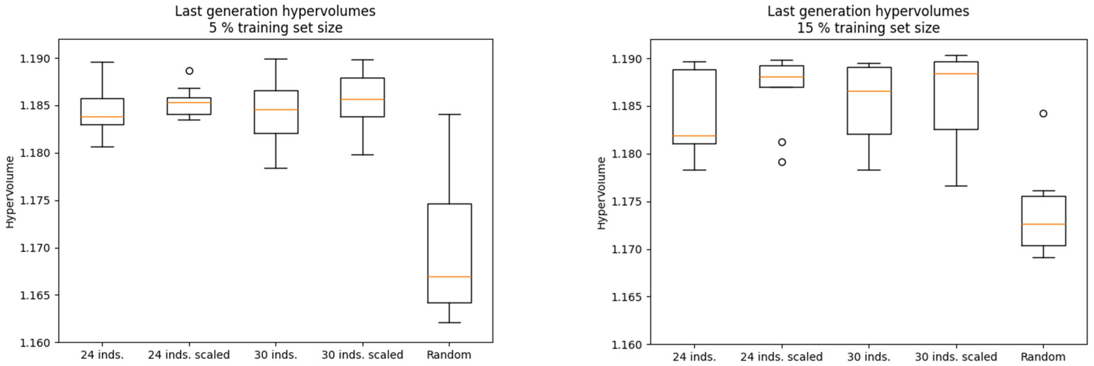
Figure 8 shows the boxplot distributions of the final HV for the 5% and 15% training set cases, shown on the left and right sides of the figure, respectively. The plots also include the distribution obtained from a random search, which performs significantly worse than the evolutionary optimization methods.

Figure 8. Boxplots of HV distribution (9 independent executions) at final population.

Table 3 and Table 4 present the results of the Friedman statistical significance test for the 5% and 15% training set cases, respectively. The p-values obtained—4.6 × 10⁻³ and 3.0 × 10⁻³—are below the significance threshold of 0.05, indicating statistically significant differences among the methods. The Bergmann–Hommel post hoc tests, shown in Table 5 and Table 6, reveal that random search performs worse than all NSGA-II optimization configurations, except for the case with a population size of 24, no fitness scaling, and a 15% training set size, where the p-value is 0.0683, slightly above the 0.05 significance level.

Table 3. Average ranking of the algorithms (comparison based on hypervolume at stopping criterion)—the lower, the better; Friedman test; 5 % training set size; p-value 0.004655.

Algorithm	Friedman Test Ranking
24_inds_scaled	2.33
30_inds_scaled	2.33
30_inds	2.67
24_inds	2.89
random	4.78

Table 4. Average ranking of the algorithms (comparison based on hypervolume at stopping criterion)—the lower, the better; Friedman test; 15 % training set size; p-value 0.003019.

Algorithm	Friedman Test Ranking
24_inds_scaled	2.11
30_inds_scaled	2.33
30_inds	2.78
24_inds	3.00
random	4.78

Table 5. Adjusted p values, Bergmann–Hommel’s post hoc procedure (comparison based on hypervolume at stopping criterion); 5 % training set size; statistical significance difference (p-value < 0.05) in italics.

i	Hypothesis	p-Value
1	24_inds_scaled vs. random	0.0104
2	30_inds_scaled vs. random	0.0104
3	30_inds vs. random	0.0185
4	24_inds vs. random	0.0451
5	24_inds vs. 24_inds_scaled	2.736
6	24_inds vs. 30_inds_scaled	2.736
7	24_inds_scaled vs. 30_inds	2.736
8	30_inds vs. 30_inds_scaled	2.736
9	24_inds vs. 30_inds	2.736
i	24_inds_scaled vs. 30_inds_scaled	2.736

Table 6. Adjusted p values, Bergmann–Hommel’s post hoc procedure (comparison based on hypervolume at stopping criterion); 15 % training set size; statistical significance difference (p-value < 0.05) in italics.

i	Hypothesis	p-Value
1	24_inds_scaled vs. random	0.00347
2	30_inds_scaled vs. random	0.00624
3	30_inds vs. random	0.0292
4	24_inds vs. random	0.0683
5	24_inds vs. 24_inds_scaled	1.398
6	24_inds_scaled vs. 30_inds	1.398
7	24_inds vs. 30_inds_scaled	1.398
8	30_inds vs. 30_inds_scaled	1.398
9	24_inds_scaled vs. 30_inds_scaled	1.531
10	24_inds vs. 30_inds	1.531

Among the NSGA-II configurations, although no statistically significant differences were found, the scaled fitness function cases consistently achieved better rankings than the non-scaled ones in both training set sizes (see Table 3 and Table 4).

In Table 7, scaled cases of the 5% and 15% training set sizes using a Friedman test are compared. The results indicate that there are no statistically significant differences between the two configurations (p-value = 0.61), although the 15% training set cases exhibit a more favorable ranking than those with 5%.

Table 7. Average ranking of the algorithms (comparison based on hypervolume at stopping criterion)—the lower, the better; Friedman test; fitness function scaled cases; p-value 0.6149.

Algorithm	Friedman Test Ranking
24_inds_scaled_15%	2.11
30_inds_scaled_15%	2.33
24_inds_scaled_05%	2.78
30_inds_scaled_05%	2.78

Based on the analysis of Figure 6 and Figure 8, as well as the Friedman ranking tables and the Bergmann–Hommel post hoc tests, the superiority of the evolutionary approach using the NSGA-II algorithm over random search is clearly demonstrated.

Detailed information on the global accumulated non-dominated front obtained from all tested experiments is provided in Table 2, including hyperparameter values, corresponding configurations, and fitness function results. The table is sorted from lowest to highest training time (and inversely, from highest to lowest validation loss). The most accurate model achieves a validation loss of approximately 0.038 million with a training time of 9.7 min, while the least accurate model requires only 0.489 min of training time but yields a validation loss of 1315 million. Notably, three models located in the lower-left corner of the Pareto front exhibit validation losses below 0.1 million and training times under 2 min and can be considered compromise solutions (solutions ranked 35th, 36th, and 37th in Table 2).

Designs obtained using the 15% training set size account for 85% of the individuals in the non-dominated front, including extreme cases. In contrast, designs generated with the 5% training set size constitute less than 15% of the front and are associated with higher validation losses and shorter training times. This suggests that a 5% training set size (3275 individuals) is insufficient for this test case, whereas a 15% training set size (9830 individuals) appears to be more appropriate.

Additionally, among the 49 non-dominated individuals, 22 correspond to the configuration with a population size of 30 and scaled fitness functions, 11 to population size 30 without scaling, 9 to population size 24 without scaling, and the remaining 7 to population size 24 with scaling.

Regarding the number of hidden layers (with search values ranging from 1 to 7), a value of 1 is only present in the leftmost solution, which corresponds to the lowest training time and the highest validation loss. Except for this case, the eight individuals with better training time have between 2 and 3 hidden layers. Individuals ranked 9th to 35th in terms of training time exhibit hidden layer counts ranging from 4 to 7. Notably, the 14 non-dominated solutions with the lowest validation loss consistently feature three hidden layers, suggesting that this configuration offers a favorable balance between accuracy and training efficiency.

Regarding the number of nodes per layer (with search values ranging from 10 to 400), the top 22 individuals, in terms of training time, have between 11 and 55 nodes per layer. Solutions ranked 23rd to 35th show values between 75 and 158 nodes, while those ranked 36th to 49th range from 204 to 373 nodes per layer. Although the trend is not strictly monotonic, there is a noticeable tendency for higher accuracy (and correspondingly longer training times) to be associated with an increased number of nodes per layer within the recommended ranges.

Regarding batch size (with search values ranging from 32 to 1024), the 19 designs with the lowest training time exhibit batch sizes between 637 and 1023. Designs ranked 20th to 28th have batch sizes ranging from 205 to 985, while those ranked 29th to 37th fall between 124 and 199. The 11 designs with the best validation loss show batch sizes between 38 and 90. Although the trend is not strictly monotonically decreasing, there is a noticeable tendency for smaller batch sizes to be associated with higher accuracy and, correspondingly, longer training times.

Regarding the alpha parameter of the Leaky ReLU activation function (with search values ranging from 0.05 to 0.5), dominant values are concentrated between 0.05 and 0.08. Specifically, 20 solutions fall within the range 0.05–0.06, 17 within 0.06–0.07, 7 within 0.07–0.08, 3 within 0.08–0.10, and 2 between 0.10 and 0.23. Notably, 75% of the values lie within the interval from 0.051 to 0.069, which is close to the lower bound of the search space.

It is also observed that the 10 individuals with the best validation loss share common characteristics: they use three hidden layers, between 204 and 373 nodes per layer, and batch sizes ranging from 38 to 71. Among these, eight originate from experiments where the fitness function was scaled. Training times for these models range from 2.43 to 9.705 min.

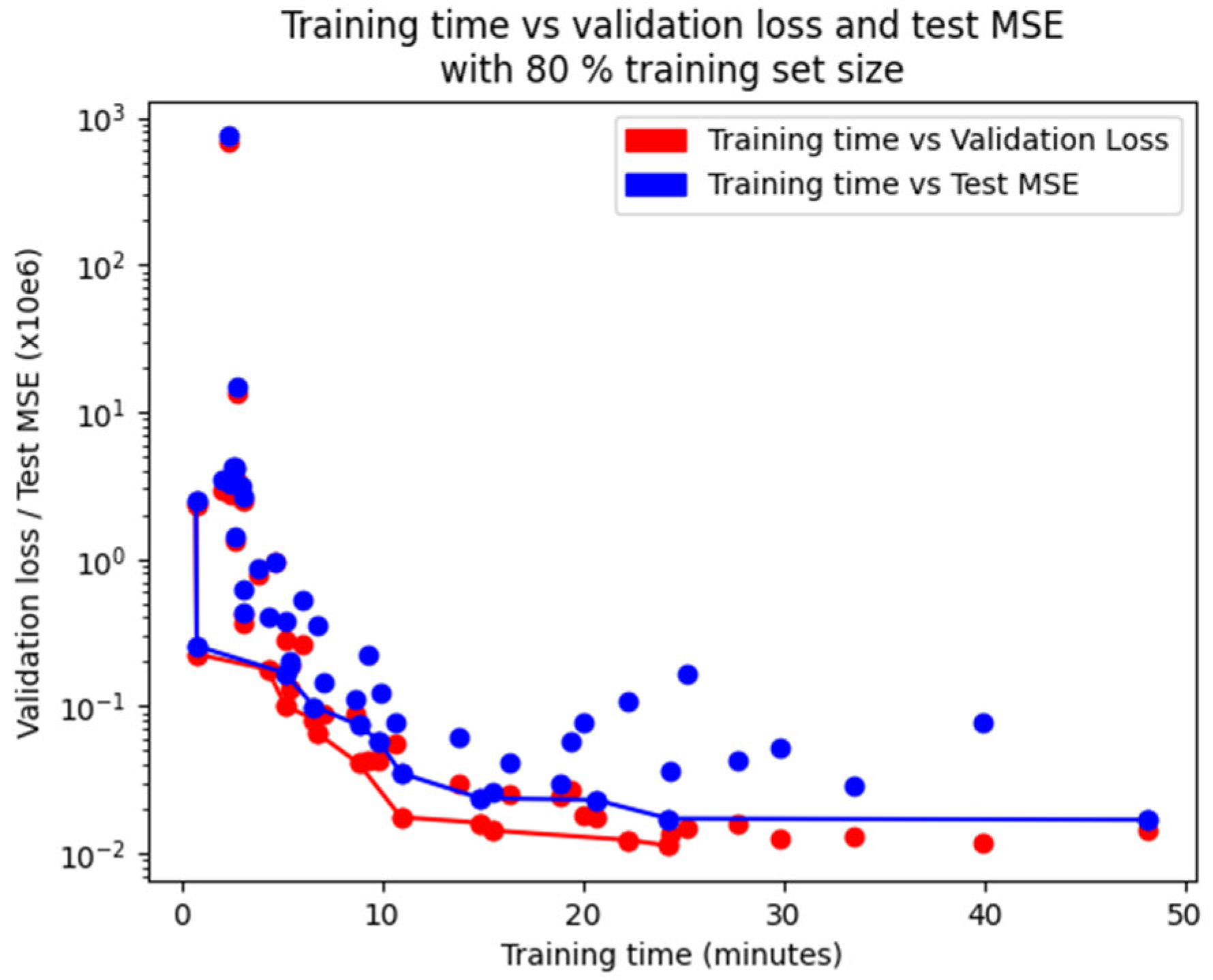
Additionally, these 49 optimum designs from the multi-objective point of view (non-dominated solutions) were taken as reference designs and trained with the full training dataset (80%, 52,429 structures). The resulting training times, validation set losses, and test set mean squared errors (MSE) are represented in Figure 9. In this figure, blue dots refer to the test set results, while red dots correspond to validation set results. Non-dominated solutions have been highlighted with connecting lines, and their detailed metrics are shown in Table 8 and Table 9. Notably, eight solutions are common to both tables.

Figure 9. Accumulated non-dominated neural network designs (as in Table 2), retrained using 80% of the dataset, and results of validation set loss and test set MSE versus training time.

Table 8. Results obtained using 80% of the dataset for training, showing training time and validation loss for non-dominated solutions (highlighted with red lines in Figure 9).

Rank	Hidden Layers	Nodes per Layer	Batch Size	Alpha	Training Time	Validation Loss (×106)
1	7	11	1012	0.0656	0.732	2.361
2	6	37	630	0.0667	0.782	0.226
3	7	37	738	0.0678	4.310	0.179
4	7	55	331	0.0634	5.167	0.101
5	5	136	932	0.0514	6.612	0.0813
6	5	136	845	0.0508	6.797	0.0654
7	5	75	124	0.0720	8.827	0.0410
8	3	259	174	0.0646	10.941	0.0176
9	3	259	176	0.0646	14.893	0.0162
10	3	294	154	0.0532	15.534	0.0143
11	3	335	94	0.0590	22.181	0.0124
12	3	373	69	0.0644	24.278	0.0113

Table 9. 80% training set size results in terms of training time and test set MSE, non-dominated solutions (blue line solutions in Figure 9).

Rank	Hidden Layers	Nodes per Layer	Batch Size	Alpha	Training Time	Test MSE (×106)
1	7	11	1012	0.0656	0.732	2.529
2	6	37	630	0.0667	0.782	0.256
3	7	55	331	0.0634	5.167	0.169
4	5	136	932	0.0514	6.612	0.0997
5	5	75	124	0.0720	8.827	0.0747
6	7	76	205	0.0728	9.862	0.0579
7	3	259	174	0.0646	10.941	0.0351
8	3	259	176	0.0646	14.893	0.0162
9	3	204	71	0.0526	20.610	0.0231
10	3	373	69	0.0644	24.278	0.0173
11	3	304	38	0.0577	48.148	0.0169

Table 9 includes 11 solutions, among which the top five most accurate designs all share a configuration of three hidden layers. The remaining designs, which exhibit lower training times but higher validation losses, have between 5 and 7 hidden layers. The number of nodes per layer increases (though not monotonically) from 11 to 304 when moving from less accurate to more accurate designs. Similarly, batch size decreases (also non-monotonically) from 1012 to 38 along the same accuracy gradient. The alpha parameter of the Leaky ReLU activation function varies within the range from 0.0514 to 0.0728, without a clear trend.

5. Conclusions

From a multi-objective point of view, the importance of hyperparameter tuning in the performance of the neural network-based metamodel has been demonstrated, considering both the accuracy and complexity of the network. Extensive experimentation across different population sizes, training set proportions, and fitness scaling strategies revealed interesting insights: larger training sets (15%) provide a greater number of designs in the accumulated non-dominated front and scaled fitness functions contribute to improved convergence and final hypervolume indicators. Statistical tests confirm the superiority of evolutionary optimization over random search.

Instead of increasing the training set size during the optimization process (highly costly), in this manuscript only the non-dominated solutions were afforded to train with the full training set (80%), as shown in Table 8 and Table 9, with satisfactory outcomes.

The analysis of the 49 non-dominated solutions reveals clear trends in hyperparameter configurations in the handled test case. Models containing three hidden layers, approximately 300 neurons each, and small batch sizes (38–71) tend to achieve the best validation performance in less time during training. Additionally, the alpha parameter of the Leaky ReLU activation function is strongly concentrated near the lower bound of the search space (0.05–0.50), suggesting its relevance in fine-tuning model behavior.

In the handled test case, the final non-dominated front (e.g., Table 9) provides solutions that combine a high number of layers (6–7) with a low number of nodes per layer (11–55) for the fastest training solutions with the best accuracy. Alternatively, solutions with three layers and a high number of nodes per layer (200–300) provide the most accurate solutions and train more quickly. This combination is obviously not optimal in terms of both accuracy and network complexity simultaneously. Thus, in other referenced studies, even when solving larger structures, a limited number of network configurations that do not take this variability into account (either considering only a small number of layers with a small number of nodes per layer or a large number of layers with a large number of nodes per layer, or even limiting the number of layers in the network to a number shown here to be insufficient, such as four) have been tested.

The use of surrogate modeling in structural engineering is linked to those needs/applications that require a high number of structural evaluations, in which case the straightforward evaluation using numerical models (as the finite element method) would be unaffordable to available computational resources when repeated many times. They could typically comprise the cases of design, control, uncertainty quantification, and optimization [38]. Although in the first three former applications a surrogate covering the whole search space would be enough, in the latter case (optimization) the exploration of the variable space is not uniform but follows a search path. Then, it would be necessary to update the surrogate model during the optimization convergence, therefore requiring many trainings of the surrogate during the search. The multi-objective neural architecture search (NAS) approach proposed here allows us to obtain the most accurate surrogate model for every training time, or alternatively seen, the lower training time model for every accuracy. Therefore, low fidelity models (less accurate but faster to train) are available in the left part of the attained non-dominated set provided by the methodology of this manuscript, while high fidelity models (more accurate but slower to train) are available in the right part of the non-dominated set. The decision-maker/engineer is able to choose the surrogate model among the non-dominated set which mostly fits his preferences/needs. This also allows a more scientifically accurate selection when designing multi-fidelity strategies that combine simultaneously high fidelity and low fidelity methods (as in, e.g., [39]).

The generalization of these conclusions would be subject to a broader study with several structures of different sizes and/or types, which could be the subject of future studies. Among the potential future lines of research, the application of this methodology to analogous structural problems that are more complex or larger in scale could be explored, including other structural types, provided that an adequate database is available. Notwithstanding the elevated computational expense associated with the network training time during the optimization process, this article proposes a methodology that assists in resolving this issue. The methodology involves the execution of the optimization with a constrained training database size and the exclusive utilization of the complete database for the training of the optimal models that appear in the non-dominated solution front.

These findings provide valuable insights into designing efficient and accurate surrogate models in structural engineering and lay the groundwork for future multi-objective neural architecture search work in this field. Using this methodology for more complex issues is a promising avenue for future research, using either the same or alternative objective functions, depending on the nature of the problem.