A Variable-Speed and Multi-Condition Bearing Fault Diagnosis Method Based on Adaptive Signal Decomposition and Deep Feature Fusion

Abstract

To address the challenges in identifying effective fault features and achieving sufficient diagnostic accuracy and robustness in variable-speed printing press bearings, where complex mixed-condition vibration signals exhibit non-stationarity, strong nonlinearity, ambiguous time-frequency characteristics, and overlapping fault features across multiple operating conditions, this paper proposes an adaptive optimization signal decomposition method combined with dual-modal time-series and image deep feature fusion for variable-speed multi-condition bearing fault diagnosis. First, to overcome the strong parameter dependency and significant noise interference of traditional adaptive decomposition algorithms, the Crested Porcupine Optimization Algorithm is introduced to adaptively search for the optimal noise amplitude and integration count of ICEEMDAN for effective signal decomposition. IMF components are then screened and reorganized based on correlation coefficients and variance contribution rates to enhance fault-sensitive information. Second, multidimensional time-domain features are extracted in parallel to construct time-frequency images, forming time-sequence-image bimodal inputs that enhance fault representation across different dimensions. Finally, a dual-branch deep learning model is developed: the time-sequence branch employs gated recurrent units to capture feature evolution trends, while the image branch utilizes SE-ResNet18 with embedded channel attention mechanisms to extract deep spatial features. Multimodal feature fusion enables classification recognition. Validation using a bearing self-diagnosis dataset from variable-speed hybrid operation and the publicly available Ottawa variable-speed bearing dataset demonstrates that this method achieves high-accuracy fault identification and strong generalization capabilities across diverse variable-speed hybrid operating conditions.

1. Introduction

Bearings, a vital part of advanced printing equipment, are exposed to varying speeds and prolonged mechanical stress, which makes them particularly vulnerable to wear, loosening, or failure over time. Even slight wear or vibration deviations in the bearings can cause instability in the printing cylinder’s operation, resulting in registration errors, ghosting, and uneven ink distribution. These issues not only affect printing accuracy and product quality but also reduce overall production efficiency and may even lead to equipment malfunction or a shortened service life. Therefore, achieving high-precision vibration state monitoring and fault diagnosis of bearings is essential to ensure the efficient and stable operation of high-end printing equipment [1,2,3].

However, the operating conditions of high-end printing equipment have become increasingly complex due to the growing demand for customized printing products. In particular, under variable-speed mixed conditions, the bearing vibration signals exhibit significant non-stationarity, strong nonlinearity, and fault feature aliasing. The fault characteristic frequencies fluctuate continuously with the changing rotational speed, and weak features are easily masked by strong noise interference. Meanwhile, the deviation between the sampling frequency and the actual bearing vibration frequency further increases the difficulty of effective feature extraction. Therefore, improving the efficiency of fault feature extraction and enhancing the adaptability of diagnostic models under complex variable-speed conditions remain urgent challenges [4,5].

At present, researchers generally employ methods based on analytical modeling, signal processing, and machine learning to investigate bearing fault diagnosis under complex operating conditions [6,7]. Analytical model–based methods primarily rely on the statistical characteristics of bearing operation data to estimate state parameters and determine fault types according to empirical rules. For example, Zhang [8] proposed an Singular Value Decomposition (SVD) -based method for fault diagnosis–assisted Variational Mode Decomposition (SVMD) combined with entropy features, which enables continuous mode extraction under unknown mode numbers and achieves effective fault diagnosis when integrated with machine learning. Similarly, Chen et al. [9] by extracting fault features through Multi-Scale Magnitude-Aware Perceptual Arrangement Entropy (MAAPE) and constructing a feature dataset, effectively addressed the non-stationarity issue in constant-speed vibration signals. Although these methods exhibit good diagnostic efficiency for single-fault conditions, their diagnostic performance becomes limited when multiple faults coexist or when operating conditions are complex, and they remain highly dependent on accurate mathematical modeling.

Signal processing–based methods typically analyze rolling bearing vibration signals using correlation functions, Fourier Transform (FT), wavelet transform, and other models to extract features such as amplitude, spectrum, and time–frequency characteristics for fault [10,11]. Among these methods, Empirical Mode Decomposition (EMD), introduced by Huang et al., is an adaptive time-frequency method ideal for analyzing nonlinear and non-stationary signals. EMD does not require predefined basis functions and decomposes signals according to their intrinsic time scales, producing Intrinsic Mode Functions (IMF) of different amplitudes. However, EMD suffers from mode mixing during decomposition [12,13]. To address this, Wu et al. introduced Ensemble EMD (EEMD), which adds white noise multiple times to alter the signal’s extreme values and then averages the resulting IMFs to eliminate the noise, partially mitigating mode mixing. Nevertheless, the added white noise can propagate downward, causing significant reconstruction errors [14]. Complete EEMD (CEEMD) adds pairs of positive and negative white noise to the signal, not only removing residual noise left after EEMD but also achieving better mode separation. However, the added noise can still propagate and affect subsequent decomposition, leading to noise residue, and the method also requires many iterations and may generate spurious modes [15]. To overcome these limitations, Torres et al. proposed Complete EEMDAN (CEEMDAN), which adds positive and negative Gaussian white noise when calculating each IMF and averages the results, effectively addressing previous [16]. On this basis, Colominas et al. developed an Improved CEEMDAN (ICEEMDAN), further enhancing decomposition performance, greatly reducing mode mixing, and minimizing the influence of spurious components on feature extraction [17,18,19]. However, ICEEMDAN still has certain limitations in practice. Since its decomposition process relies on noise addition and multiple iterations, parameter selection and optimization are critical. The decomposition performance of ICEEMDAN is influenced by factors such as noise amplitude, decomposition levels, and the number of iterations; different parameter settings may lead to instability in mode decomposition or deviations in feature extraction.

Learning and adjusting model parameters through optimization algorithms can effectively improve model performance. Among them, the Crested Porcupine Optimizer (CPO) algorithm, as a novel optimization method, possesses strong global search ability and low computational complexity, and can adaptively adjust its search strategy, effectively avoiding local optima. Compared with traditional algorithms, CPO demonstrates higher efficiency, accuracy, and adaptability in high-dimensional signal processing and feature selection. For instance, Lv et al. [20] applied CPO to optimize two key parameters of the Minimum Noise Amplitude Deconvolution (MNAD) model, achieving efficient global search and parameter optimization, enabling rapid convergence in complex optimization problems while effectively avoiding local optima. Although these methods can stably extract fault features based on theoretical models, relying on single feature indicators is often insufficient to comprehensively and effectively capture the complex fault information present in vibration signals.

Machine learning, particularly deep learning, has attracted attention for its ability to diagnose faults under complex conditions thanks to its self-learning capabilities. These methods can uncover deep, nonlinear features and enable end-to-end fault diagnosis, exhibiting strong adaptability and robustness [21,22,23]. Among them, Residual Neural Networks (ResNets) introduce skip connections to construct deep neural networks, which can partially alleviate model degradation and gradient vanishing problems. However, training these models requires large labeled datasets, often unavailable in practice [24,25,26,27]. To address this, Luo et al. [28] proposed a constant-speed bearing fault diagnosis model combining Quadratic Convolutional Neural Network (QCNN) with ResNet. The model introduces nonlinear convolutional structures to enhance the extraction of key features, while residual connections mitigate gradient vanishing during deep network training, effectively improving fault recognition accuracy and robustness. Similarly, Li [29] proposed a model combining Convolutional Neural Network (CNN) with Knowledge-Augmented Networks (KANs). Raw vibration signals are transformed into 2D time–frequency images via Continuous Wavelet Transform (CWT), then features are extracted using CNN-KANs, and a Feature Aggregation Network (FAN) further fuses multi-layer features. Finally, a diffusion network is used to generate data to address the small-sample problem. However, such machine learning approaches are highly data-dependent and suffer from limited interpretability and generalization ability and are often difficult to integrate with physical mechanisms. As a result, efficient fault diagnosis of bearings under mixed operating conditions and unknown environments remains a significant challenge in complex industrial scenarios.

Therefore, deep integration of data-driven fault feature learning with signal analysis methods that capture the underlying physical mechanisms can effectively address the aforementioned challenges [30,31]. Zaman et al. [32] proposed a multimodal fault diagnosis framework for milling machines that combines autoencoders (AE) with vibration signals, leveraging their complementary advantages to enhance detection capability. Time–frequency images are generated via CWT and fed into parallel ResNet-50 networks for feature extraction, with an interleaved fusion strategy to integrate multimodal information, and final fault classification is achieved through fully connected layers. However, this approach primarily targets constant-speed conditions and does not account for fault feature variations under variable-speed operation. Chen [33] directly uses raw vibration signals as input, with dual CNN automatically extracting frequency-domain features. Nonetheless, this method pays insufficient attention to critical frequency bands, and under complex operating conditions or noisy environments, it is prone to feature mixing and reduced recognition accuracy. Wang [34] proposed a bearing fault diagnosis method combining multimodal feature extraction with 1D-CNN to overcome challenges of single-modal vibration features and low classification accuracy. However, this method mainly relies on the independent processing of vibration and acoustic signals, lacking joint modeling and fusion of time-domain and frequency-domain features, which limits its adaptability under complex operating conditions.

Hybrid models combining CNN and (Recurrent Neural Networks) RNN variants have been widely applied in bearing fault diagnosis. Han [35] proposed a deep learning model integrating CNN, LSTM, and Gated Recurrent Unit (GRU) networks, where CNN extracts spatial features, Long Short-Term Memory network (LSTM) captures long-term dependencies, and GRU handles short-term dynamic changes, achieving high-precision fault recognition under various noisy environments. MF et al. [36] proposed an improved ResNet with attention and multi-scale feature fusion to enhance feature extraction and diagnostic robustness under complex conditions. However, these methods still face limitations under mixed operating conditions and variable-speed scenarios. Single-branch networks struggle to simultaneously capture multi-dimensional time-domain and frequency-domain features, and complex signal noise and feature mixing can lead to reduced diagnostic accuracy and insufficient robustness.

In summary, this paper proposes a fault diagnosis method for variable-speed, multi-condition bearing vibration based on CPO-adaptive optimized ICEEMDAN signal decomposition and ResNet18-GRU fused time–series–image dual-modality deep feature extraction, aiming to improve diagnostic accuracy and adaptability under complex operating conditions in printing equipment. First, the CPO algorithm is introduced to adaptively search for the optimal noise amplitude and ensemble number in ICEEMDAN, enabling effective signal decomposition. IMF components are then selected and recombined based on correlation coefficients and variance contribution rates to enhance fault-sensitive information. Next, multi-dimensional time-domain features are extracted in parallel and time–frequency images are constructed to form a dual-modality input of time series and images, strengthening fault representation across different dimensions. Finally, a dual-branch deep learning model is constructed: the temporal branch employs a Gated Recurrent Unit (GRU) to capture feature evolution trends, while the image branch uses SE-ResNet18 with an embedded channel attention mechanism to extract deep spatial features. The fused multi-modal features are then used for fault classification and recognition. Experiments conducted on both a self-collected variable-speed mixed-condition bearing dataset and the public Ottawa variable-speed bearing dataset demonstrate that the proposed method achieves high-precision fault recognition and strong generalization performance under various variable-speed and mixed operating conditions.

2. Theoretical Background

2.1. CPO-Optimized ICEEMDAN-Based Adaptive Nonstationary Signal Decomposition Method

2.1.1. CPO

The CPO is a nature-inspired optimization algorithm based on crested porcupines’ defensive behaviors—visual, acoustic, odor, and physical—which are abstracted into global and local search strategies through population initialization and mathematical modeling.

(1)

Population Initialization

Each crested porcupine individual represents a candidate solution, and the population is initialized using the following formula:

$$x_i=L_{\mathrm{L}}+B(U_{\mathrm{L}}-L_{\mathrm{L}})$$

(1)

In the formula, $i=1,2,\dots ,N$, where $N$ is the population size; $x_i$ represents the position of the $i$ individual in the population; $B$ is a random number between [0, 1]; $L_{\mathrm{L}}$ is the lower limit of the search interval; $U_{\mathrm{L}}$ is the upper limit of the search interval.

During the optimization process of the CPO algorithm, some crested porcupine individuals temporarily leave the population and later rejoin to enhance population diversity, thereby improving convergence efficiency. This process is mathematically expressed as follows:

$$N=N_{\min }+(N-N_{\min })\left(1-\left({\displaystyle \frac{t\mathrm{bmod}\frac{t_{\max }}{D}}{\frac{t_{\max }}{D}}}\right)\right)$$

(2)

In the formula: $N_{min}$ is the minimum number of individuals in the newly generated population, generally 0.8 times of $N$; \(t\) is the current iteration number; bmod is the modulo operation; $t_{max}$ is the maximum iteration number; $D$ is the number of cycles, generally 2.

(2)

Visual Defense Strategy

This decision-making process is simulated using normally distributed random numbers, and its mathematical model is expressed as follows:

$$x_i^{t+1}=x_i^t+a_1\times \mid 2\times a_2\times x_{\mathrm{Best}}^t-y_i^t\mid$$

(3)

$$y_i^t={\displaystyle \frac{x_i^t+x_z^t}{2}}$$

(4)

In the formula: $z$ is a random integer in [1, N].

(3)

Acoustic Defense Strategy

The corresponding mathematical model is formulated as follows:

$$x_i^{t+1}=(1-V_1)x_i^t+V_1(x_{z_1}^t+S_i^t(x_{z_1}^t-x_{z_3}^t)-a_3\delta {\gamma }_t{S}_i^t)$$

(5)

In the formula: $V_1$ is a random number, taking 0 or 1; $y$ is the position of the natural enemy; $a_3$ is a random number in [0, 1]; $x_{z_1}^t$ and $x_{z2}^t$ are the positions of two randomly selected crested porcupines.

(4)

Olfactory Defense Strategy

The corresponding mathematical model is formulated as follows:

$$x_i^{t+1}=(1-V_1)x_i^t+V_1(x_{z_1}^t+S_i^t(x_{z_2}^t-x_{z_3}^t)-a_3\delta {\gamma }_t{S}_i^t)$$

(6)

In the formula: $S_i^t$ is the odor diffusion factor; $z_3$ is a random integer in [1, N]; $\delta$ is a parameter controlling the search direction; ${\gamma }_t$ is the defense factor. $\delta$ and ${\gamma }_t$ are defined as follows:

$$\delta =\left\{\begin{array}{c}1,\mathrm{if} B⩽0.5\\ -1,\mathrm{else}\end{array}\right.$$

(7)

$${\gamma }_1=2B{\left(1-{\displaystyle \frac{t}{t_{\max }}}\right)}^{{\displaystyle \frac{t}{t_{\max }}}}$$

(8)

(5)

Physical Attack Defense Strategy

The corresponding mathematical model is formulated as follows:

$$x_i^{t+1}=x_{\mathrm{Best}}^t+(\alpha (1-a_4)+a_4)(\delta x_{\mathrm{Best}}^t-x_i^t)-a_5\delta {\gamma }_t{F}_i^t$$

(9)

In the formula: $\alpha$ is the convergence factor; $a_4$ and $a_5$ are random numbers in [0, 1]; $F_i^t$ is the average force of crested porcupines attacking the $i$ predator, which is calculated according to the inelastic collision theorem.

2.1.2. ICEEMDAN

Define $x$ as the signal to be decomposed, $E_k(·)$ represents the $k$ order modal component generated by EMD, $N(·)$ represents the local mean value of the generated signal, and $w^{(i)}$ represents Gaussian white noise.

(1)

Add white noise to the original data sequence

$$X_1^{(i)}=x+e_1{E}_1(w^{(i)}),(i=1,2,\dots n)$$

(10)

In the formula, $x$ is the original signal; $e_1$ is the noise standard deviation of the first decomposed signal; $w^{(i)}$ is a series of Gaussian white noises.

(2)

Calculate the first decomposition residual

$$r_1=⟨X_1^{(i)}-E_1(X_1^{(i)})⟩$$

(11)

Among them: $⟨·⟩$ represents taking the average value.

(3)

Obtain the first component by subtracting the first calculated residual $r_1$ from the original signal $x$:

$$IM{F}_1=x-r_1$$

(12)

(4)

Estimate the second residual as the mean value of a series of $r_1+e_2{E}_2(w^{(i)})$ and obtain the second component:

$$IM{F}_2=r_1-r_2=r_1-⟨(r_1+e_2{E}_2({\omega }^i))⟩$$

(13)

(5)

The residual $r_k$ of the $k$ order modal:

$$r_k=⟨X_k^{(i)}-E_k(X_k^{(i)})⟩$$

(14)

(6)

Calculate the $k$ order intrinsic mode function $IM{F}_k$

$$IM{F}_k=r_{k-1}-r_k$$

(15)

In the formula, $k$ is the total number of IMF.

(7)

Return to step 5 to calculate $r_{k+1}$.

2.1.3. Selection Criteria for IMF Components

This study uses the parson correlation coefficient and variance contribution rate to reconstruct IMF components.

(1)

Correlation Coefficient

For two variables X and Y, the correlation coefficient is expressed as:

$${\mathit{\gamma }}_{X,Y}={\displaystyle \frac{{\displaystyle {\sum }_{\mathrm{i}=1}^{\mathrm{n}}(X_{\mathrm{i}}-\overline{X})(Y_{\mathrm{i}}-\overline{Y})}}{\sqrt{{\displaystyle {\sum }_{i=1}^n(X_{\mathrm{i}}-\overline{X}{)}^2{\displaystyle {\sum }_{i=1}^n(Y_{\mathrm{i}}-\overline{Y}{)}^2}}}}}$$

(16)

In the formula, $\overline{X}$ and $\overline{Y}$ are the means of variables $X$ and $Y$, respectively, and $n$ is the sample size.

(2)

Variance Contribution Rate

The VCR is defined as follows:

$$mse(k)={\displaystyle \frac{{\left(IM{F}_k-E\right)}^2}{n{\sigma }^2}}$$

(17)

In the formula, $E$ and ${\sigma }^2$ are the mean and variance of the original signal sequence, respectively.

The calculation formulas for the thresholds of both indicators can be unified as follows:

$$t={\displaystyle \frac{P_{\max }}{10\ast {\left(P_{\max }\right)}^{-3}}}$$

(18)

In the formula: $P_{\max }$ is the maximum value of the corresponding index.

2.2. ResNet18-GRU Parallel Fusion Network

2.2.1. ResNet18 Network Principles

Let the input-output relationship of a residual connection be denoted as $G(x)$, which is expressed as follows:

$$G(x)=X+F(X)$$

(19)

In the formula, $X$ represents the input, $F(x)$ represents the output, and $F$ represents operations such as convolution and activation.

The output of the residual module needs to add the Re-Lu activation function after $X+F(x)$ to obtain an accurate output result. Moreover, since there may be a dimension difference between $X$ and $G(X)$ in the residual connection, the residual network will first perform a convolution operation on $X$, which is specifically expressed as follows:

$$G(x)=X+F(X)$$

(20)

In the formula, $h$ represents the convolution operation.

Compared with the serial structure of ordinary convolutional neural network models, the ResNet model adds a skip connection structure that can directly add input and output. This structure not only makes the data obtained during model training more complete but also makes the training efficiency of the convolutional neural network model higher and the detection effect better, greatly improving the performance of the convolutional neural network model.

2.2.2. GRU Network Principles

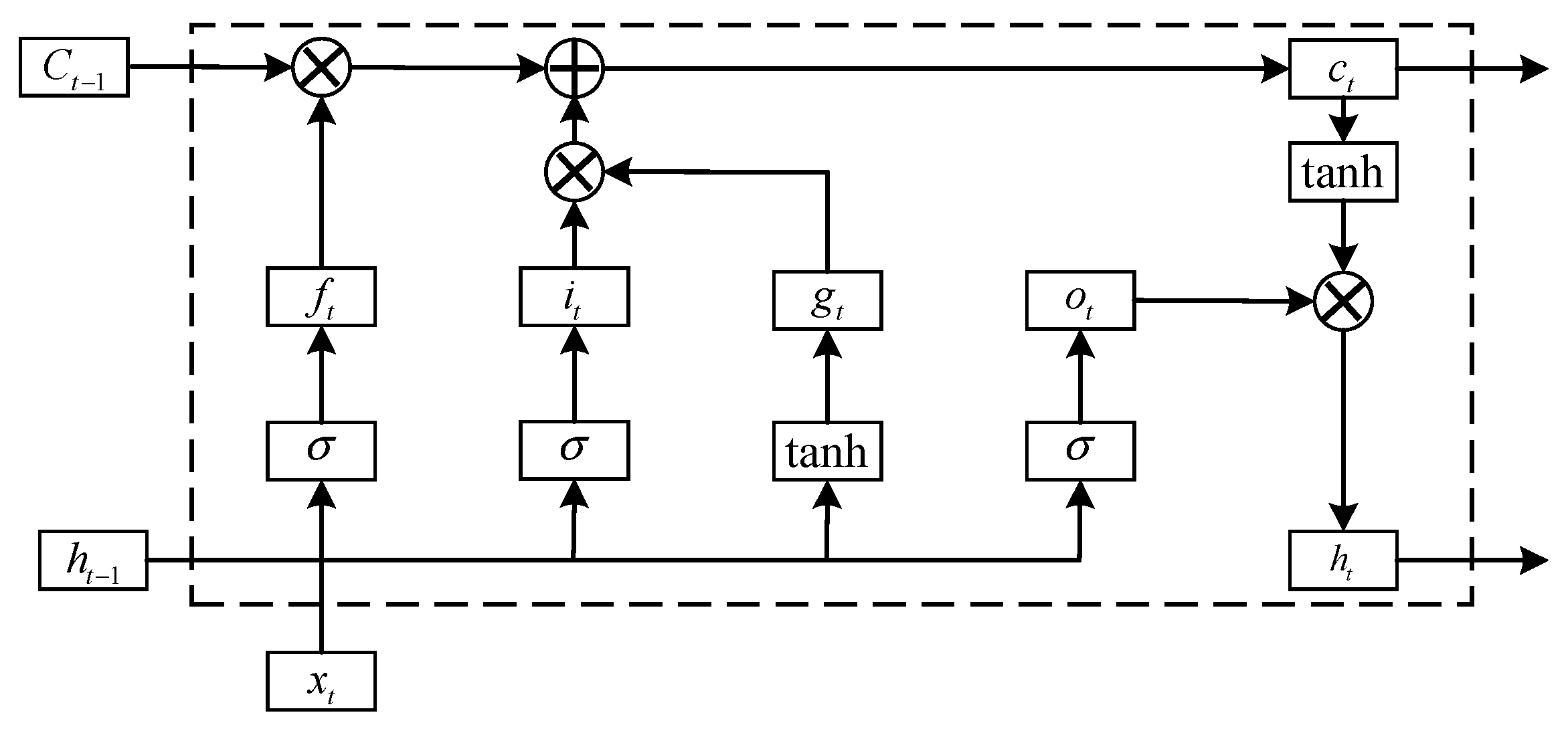
Figure 1 shows the LSTM network, which regulates information flow via three gates: forget, input, and output, with the following functions:

$$\left\{\begin{array}{l}{i}_t=\sigma \left(W_{\mathrm{ix}}{x}_t+W_{\mathrm{ih}}{h}_{t-1}+b_{\mathrm{i}}\right)\\ f_t=\sigma \left(W_{\mathrm{fx}}{x}_t+W_{\mathrm{f}h}{h}_{t-1}+b_{\mathrm{f}}\right)\\ g_t=\tanh \left(W_{\mathrm{gx}}{x}_t+W_{\mathrm{gh}}{h}_{t-1}+b_{\mathrm{g}}\right)\\ o_t=\sigma \left(W_{\mathrm{ox}}{x}_t+W_{\mathrm{oh}}{h}_{t-1}+b_{\mathrm{o}}\right)\\ c_t=f_t\otimes c_{t-1}+i_t\otimes g_t\\ h_t=o_t\otimes \tanh \left(c_t\right)\end{array}\right.$$

(21)

Figure 1. Long short-term memory network.

In the formula, $t$ is the current time; $g_t$ is the cell unit; $h_t$ is the hidden state; $x_t$ is the input information at the current time; $W_{pq}$ is the weight of the connection between $p$ and $q$, and the values of $p$ and $q$ are \(f \), $f, i, o, x, g, h$, representing the forget gate, input gate, output gate, input information, cell unit, and hidden state, respectively; $b_s$ is the bias parameter of the control gate s; $\sigma$ is the sigmoid function, which obtains a gating signal in the range of 0–1; \tanh is the activation function.

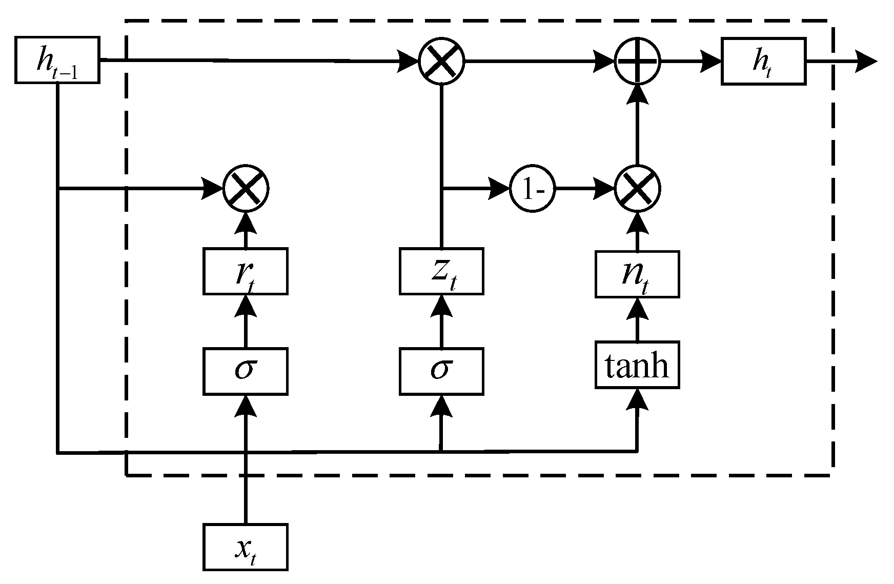
The structure of the GRU is shown in Figure 2.

$$\left\{\begin{array}{l}{r}_t=\sigma \left(W_{\mathrm{rx}}{x}_t+W_{\mathrm{rh}}{h}_{t-1}+b_{\mathrm{r}}\right)\\ z_t=\sigma \left(W_{\mathrm{zx}}{x}_t+W_{\mathrm{zh}}{h}_{t-1}+b_{\mathrm{z}}\right)\\ n_t=\tanh (W_{\mathrm{nx}}{x}_t+W_{\mathrm{nh}}{h}_{t-1}+b_{\mathrm{n}})\\ h_t=(1-z_t)n_t+z_t{h}_{t-1}\end{array}\right.$$

(22)

Figure 2. Structure of GRU gating unit.

In the formula: $r_t$ is the reset gate; $z_t$ is the update gate; $n_t$ is the new gate; the subscripts $r, z, n$ represent the reset gate, update gate, and new gate, respectively.

It can be seen from Formula (22) that GRU can complete both forgetting and memory functions simultaneously with the update gate $z_t$. GRU is more efficient and concise than LSTM.

2.2.3. Principles of the SE Attention Mechanism

When SE Net is embedded into the convolutional layers of ResNet18, the workflow can be divided into four steps:

(1)

A feature map $u$ is generated through the transformation $F_{tr}$ process. Among them, $F_{tr}:x\to u,x\in R^{H^{\prime }{W}^{\prime }{C}^{\prime }},u\in R^{HWC}$, the convolution kernel is $V=\left[v_1,v_2,\dots ,v_c\right]$, and the output is $u=\left[u_1,u_2,\dots ,u_c\right]$ as shown in the formula:

$$u_C=v_C\ast x={\displaystyle \sum _{S=1}^{C^{\prime }}{v_C}^S\ast x^S}$$

(23)

In the formula, $\ast$ is the convolution kernel, and $v_C$ is the c convolution kernel ${v_C}^S$, a 2D convolution kernel with S channels.

(2)

The feature maps from Conv_1 are spatially compressed without changing the channel number. Each 2D feature channel is reduced to a scalar via global average pooling, as shown below:

$$z_C=F_{sq}\left(u_C\right)={\displaystyle \frac{1}{h\times w}}\sum _{i=1}^h\sum _{j=1}^w{u}_C\left(i,j\right)$$

(24)

In the formula: Z_C global feature, $z\in R^C$; $u_C \left(i, j\right)$ represents the pixel feature in the $i$ row and $j$ column; $F_{sq}$ is a compression operation.

(3)

After obtaining global channel features, excitation is performed using a gating mechanism with two fully connected layers. The first layer with ReLU reduces dimensions and introduces nonlinearity, while the second layer with Sigmoid restores dimensions and produces channel weights, as shown below:

$$s=F_{ex}\left(z,W\right)=\sigma \left[g\left(z,W\right)\right]=\sigma \left[W_2\delta \left(W_{1}z\right)\right]$$

(25)

In the formula, $s$ is the output of the excitation operation; $W1, W2$ are two fully connected layers, $W_1\in R^{{\displaystyle \frac{C}{r}}\times C}$, $W_1\in R^{C\times {\displaystyle \frac{C}{r}}}$. $F_{ex}$ is the excitation operation, and $\sigma$, $\delta$ are Sigmoid and ReLU activation functions, respectively.

(4)

Each channel’s learned weight is multiplied with its corresponding feature map to enhance important features and suppress less relevant ones, as shown below:

$$\widetilde{x_c}=F_{scale}(s_C,u_C)=s_C{u}_C$$

(26)

3. Fault Diagnosis Model Based on CPO-ICEEMDAN and ResNet18-GRU

3.1. Time-Frequency and Temporal Feature Extraction

3.1.1. Generation of Images via Generalized S-Transform

For each sample signal $x\left(t\right)$, the Generalized S-transform is used to generate a two-dimensional time-frequency image $GST\left(\tau ,f\right)$, which is saved as a PNG image. Figure 3 shows that signal energy distribution in time–frequency reveals differences among fault types.

Figure 3. Time-Frequency Diagrams of Different Fault Types Based on Generalized S-transform.

3.1.2. Time-Domain Feature Extraction

Time-domain features, such as the mean and standard deviation (listed in Table 1), are extracted from bearing vibration signals to capture their statistical and dynamic characteristics, providing comprehensive information for accurate and robust fault diagnosis.

Table 1. Time-domain features.

Time—Domain Features	Equation	Time—Domain Features	Equation
Mean value	$\overline{S}={\displaystyle \frac{1}{N}}{\displaystyle \sum _{i=1}^N{S}_i}$	RMS	$\mathrm{RMS}={\left({\displaystyle \frac{1}{N}}{\displaystyle \sum _{i=1}^N{S}_i^2}\right)}^{{\displaystyle \frac{1}{2}}}$
Standard deviation	${\rho }_t={\left({\displaystyle \frac{1}{N}}{{\displaystyle \sum _{i=1}^N{\left(s_i-\overline{s}\right)}_i}}^2\right)}^{{\displaystyle \frac{1}{2}}}$	crest factor	$S_{\max }/RMS$
Skewness	${\displaystyle \frac{1}{N}}{\displaystyle \sum _{i=1}^N\frac{{(s_i-\overline{s})}^3}{{{\rho }_t}^3}}$	Amplitude factor	$RMS/\left({\displaystyle \frac{1}{N}}{\displaystyle \sum _{i=1}^N\left|s_i\right|}\right)$
Kurtosis	${\displaystyle \frac{1}{N}}{\displaystyle \sum _{i=1}^N\frac{{(s_i-\overline{s})}^4}{{{\rho }_t}^3}}$	Waveform factor	$S_{\max }/\left({\displaystyle \frac{1}{N}}{\displaystyle \sum _{i=1}^N\left|s_i\right|}\right)$
Maximum minimum	$S_{\max },S_{\min }$	Impact factor	$S_{\max }/{\left({\displaystyle \frac{1}{N}}{\displaystyle \sum _{i=1}^N\left|s_i\right|}\right)}^2$
Peak-to-peak value	$S_{\max }-S_{\min }$	Margin factor	${\displaystyle \sum _{i=1}^N{S}_i^2}$

Each sample’s image and temporal features correspond to its label. The images are used as inputs to the ResNet18 branch, while the 13-dimensional temporal features serve as inputs to the GRU branch. Both branches are subsequently fed into the parallel ResNet18-GRU network for classification modeling.

3.2. Fault Diagnosis Model Architecture and Workflow Diagram

Based on the aforementioned fault diagnosis model combining CPO-ICEEMDAN and ResNet18-GRU, this section designs a fault diagnosis framework that integrates signal decomposition and reconstruction, time-domain feature extraction, generalized S-transform, and ResNet18-GRU. Figure 4 shows the process diagram, and Figure 5 presents the flowchart. The first step involves collecting bearing vibration data from a simulated printing device. The collected raw vibration signals are then decomposed and reconstructed using CPO-optimized ICEEMDAN to extract the effective signal components. Subsequently, time-domain features are extracted from the reconstructed signals, and generalized S-transform is applied to obtain time–frequency images, achieving multi-dimensional signal representation. Finally, the time-domain features and time–frequency image features extracted by the ResNet18-based convolutional neural network are fused and input into the GRU network for sequential modeling and fault classification, enabling accurate diagnosis of bearing fault conditions.

Figure 4. Flowchart of CPO-ICEEMDAN-ResNet18-GRU.

Figure 5. Fault Diagnosis Flowchart of Variable Operating Condition Bearings Based on CPO-ICEEMDAN and ResNet18-GRU.

The steps involved are as follows:

(1)

Data acquisition: Collect bearing fault signals under varying speed conditions on a simulated test rig, covering multiple conditions.

(2)

CPO initialization: Initialize the CPO algorithm by setting population size, maximum iterations, search space dimensions, and related parameters.

(3)

ICEEMDAN decomposition using individual parameters: Execute ICEEMDAN decomposition on the raw vibration signal using the parameters corresponding to the current individual (candidate solution) to obtain intrinsic mode function (IMF) components.

(4)

Fitness calculation and recording: Evaluate the effectiveness of the current parameter combination by computing the fitness function from the decomposition results, and record the resulting fitness value.

(5)

Check maximum iterations: If the maximum iteration number is not reached, return to Step 3 to update individual parameters and continue decomposition; otherwise, output the current optimal parameter combination.

(6)

ICEEMDAN decomposition: Apply ICEEMDAN decomposition to the raw signal using the optimized parameters to obtain multiple IMF components.

(7)

IMF component selection: Analyze the correlation and variance contribution of each IMF component relative to the original signal, selecting the components containing major fault information and discarding irrelevant components.

(8)

Reconstructed denoised signal: Reconstruct the selected relevant IMF components to form a denoised signal with improved quality.

(9)

Signal feature extraction: Extraction of Time-Domain Features and Construction of Frequency-Domain Images

(10)

Dual-branch input construction: Input the time-domain features and time–frequency images into two parallel branches: a GRU branch for sequential features and a ResNet18 branch for image features.

(11)

Spatial feature extraction: Extract spatial features from the time–frequency images using the ResNet18 convolutional neural network.

(12)

Sequential dependency feature extraction: Model the time-domain feature sequence using the GRU network to capture temporal dependencies.

(13)

Feature fusion: Fusion of time-domain and frequency-domain features

(14)

Fully connected + Softmax layer: Pass the fused features through a fully connected layer and a Softmax classification layer to output the probability of each fault category.

(15)

Output fault diagnosis results: Determine the bearing fault condition based on the classification probabilities.

(16)

Evaluation metrics: Evaluate the diagnosis results by calculating accuracy, recall, F1-score, and other metrics to validate model performance.

(17)

End: The fault diagnosis process concludes.

4. Experiments and Results Analysis

4.1. Self-Collected Dataset

The experiment was conducted on a bearing fault diagnosis test rig simulating printing equipment. The test rig mainly consists of an AC motor, a coupling, an accelerometer, a magnetic powder controller, and a tachometer, as shown in Figure 6. Variable-speed conditions were employed: the motor started from a stationary state and accelerated uniformly to 1800 r/min within 0–5 s. Additionally, a variable-speed experiment with an acceleration duration of 0–10 s was performed to capture vibration response data at different acceleration stages. Vibration signals were collected in real time using an accelerometer mounted on the top of the coupling’s output end, measuring the bearing’s vertical acceleration response. The fault types included five categories: normal, inner race fault, outer race fault, rolling element fault, and compound fault. During data acquisition, experiments under different fault conditions were repeated to obtain representative vibration signals under variable-speed conditions.

Figure 6. Bearing Fault Simulation Test Rig.

Bearing vibration signals collected under variable-speed conditions were used, encompassing five operating states. The raw signals were sampled at 2 kHz, with acquisition durations of 0–5 s and 0–10 s, corresponding to 50,000 and 76,000 data points, respectively. Due to substantial speed variations across different time segments under variable-speed conditions, a representative and stable analysis region with pronounced fault feature expression was selected. Specifically, 20,000 to 50,000 data points (corresponding to approximately 1–2.5 s) were chosen as the main analysis interval, as shown in Figure 7.

Figure 7. Data selection interval chart.

To ensure consistency in feature extraction and fairness in model training, the analysis interval was uniformly selected as data points 20,000 to 50,000 across all five operating conditions. This interval not only covers a typical variable-speed process but also corresponds to a relatively stable system operation state, facilitating accurate extraction of effective features and enhancing the scientific rigor and reliability of fault classification. As shown in Figure 7a–e, the selected interval contains representative vibration responses for the five bearing states, including the normal condition, the inner race fault, the outer race fault, the rolling element fault, and the compound fault.

The initial segment of the signal (0–1 s, corresponding to the first 20,000 data points) usually contains non-stationary factors such as motor startup, acceleration fluctuations, and transient impacts. The amplitude fluctuates greatly and the spectral structure is complex, which can obscure true fault features and interfere with subsequent analysis. To avoid these effects, this study discards the initial segment and focuses on the middle segment (1–2.5 s), corresponding to data points 20,000–50,000. This analysis interval exhibits a good signal-to-noise ratio and dynamic characteristics, clearly reflecting the key characteristic frequency variations in bearing faults.

Specifically, for inner race faults, the characteristic frequency (BPFI) varies linearly with rotational speed. In this interval, it manifests as energy gradually spreading along the frequency direction, making it suitable for extracting harmonic-related information via time–frequency analysis methods such as the S-transform. Meanwhile, the amplitude is stable, and the frequency structure is clear, which helps improve the model’s ability to identify various fault types. Moreover, the data length of 30,000 points is moderate, facilitating the use of a sliding-window approach to generate training samples. This approach meets the sample size requirements of deep learning models while controlling computational costs, providing high-quality, uniformly formatted data for image generation, feature extraction, and CNN+GRU network modeling.

In summary, selecting data points 20,000–50,000 balances signal characteristics and design considerations for efficient, robust fault diagnosis under variable speeds.

The dataset comprises five bearing states. For each state, vibration signals of two durations (0–5 s and 0–10 s) were collected, resulting in a total of ten categories, as shown in Table 2. All samples were acquired under variable speed conditions ranging from 0 to 1800 rpm. Each category contains 1200 samples, of which 840 are used for training and 360 for testing, ensuring balance and representativeness in both signal duration and fault type. The characteristic frequencies for each fault state are as follows: inner race fault, 164.74 Hz; outer race fault, 101.44 Hz; rolling element fault, 66.29 Hz; compound fault, 332.47 Hz; while the normal state contains no characteristic frequency.

Table 2. Dataset fault labels.

Label	Bearing State	Training Set	Sample Set	Frequency
1	normal (0–5 s)	420	180	-
2	inner (0–5 s)	420	180	164.74
3	outer (0–5 s)	420	180	101.44
4	roll (0–5 s)	420	180	66.29
5	mix (0–5 s)	420	180	332.47
6	normal (0–10 s)	420	180	-
7	inner (0–10 s)	420	180	164.74
8	outer (0–10 s)	420	180	101.44
9	roll (0–10 s)	420	180	66.29
10	mix (0–10 s)	420	180	332.47

4.2. Experimental Results and Analysis of the Self-Collected Dataset

4.2.1. Decomposition and Reconstruction of Bearing Vibration Signals

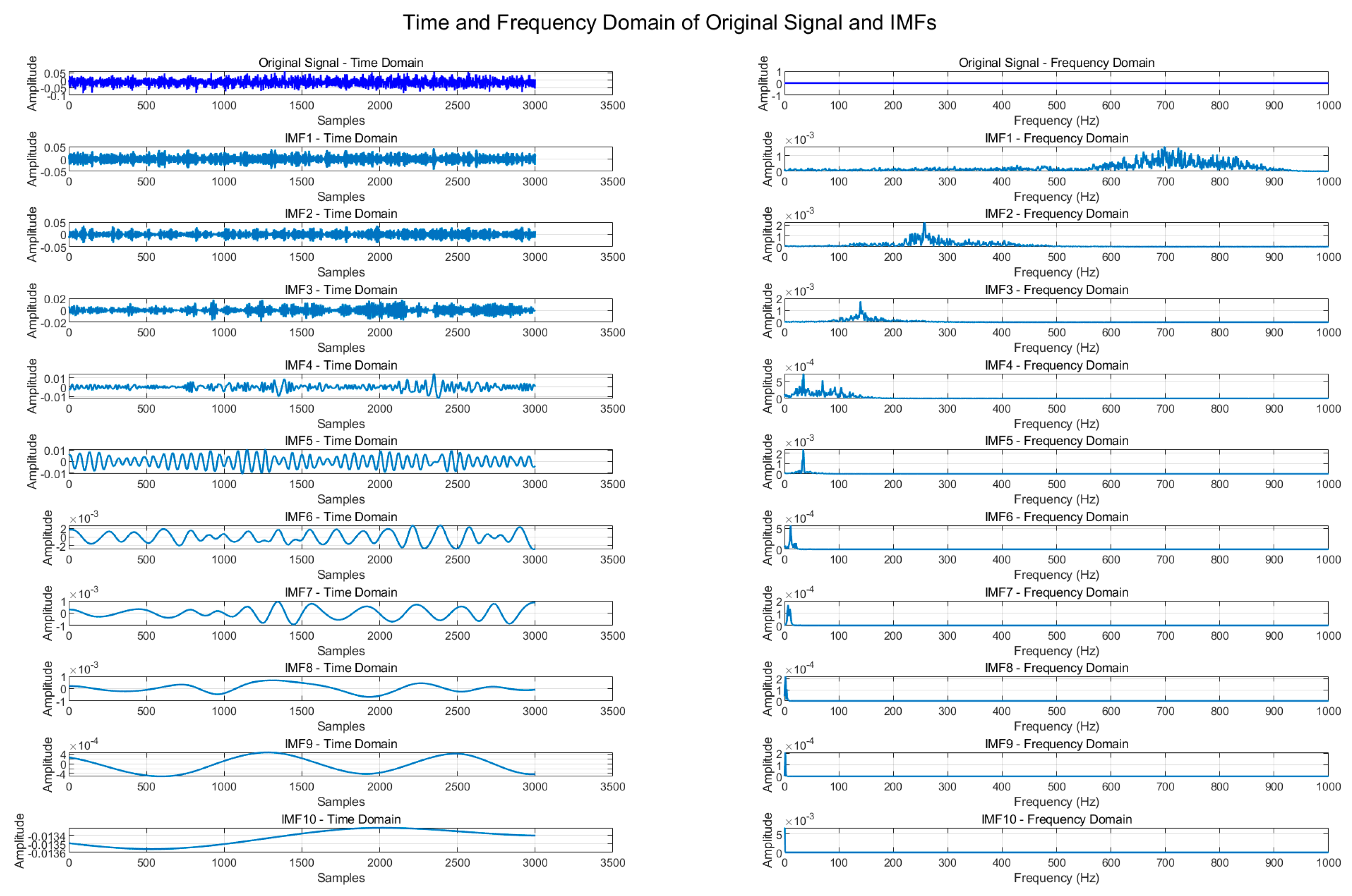
The CPO-ICEEMDAN method was applied to decompose the vibration signals corresponding to the five fault types. Ultimately, each signal was decomposed into nine intrinsic mode functions (IMFs) and one residual component. Figure 8 illustrates the original signals and their IMF components in both the time and frequency domains. In the time-domain plots, the waveforms of the original signal and each IMF component reveal different characteristics after decomposition, with each IMF reflecting local variations in the signal within a specific frequency band. Observing the time-domain signals clearly shows the distribution of different frequency components within the signal.

Figure 8. Time-Frequency Domain of Original Signal and IMF Components.

The frequency-domain plots on the right further reveal the distribution of each IMF component across frequencies, showing how energy is distributed in different frequency ranges. Figure 9 presents the convergence process of the CPO optimization. The figure shows the convergence curve of the CPO algorithm over multiple iterations. The results indicate that after approximately 20 iterations, the optimization process stabilizes, with the fitness value gradually decreasing toward the optimal solution.

Figure 9. Convergence Curve of CPO Optimization.

To avoid feature redundancy, appropriate IMF components were selected using the PCC and VCR method. Taking the outer race fault signal as an example, the correlation coefficients and variance contribution rates between each IMF component and the original signal were calculated using Equations (16) and (17), with the specific values presented in Table 3 and Table 4. Based on the results computed from Equation (18), IMF components 1 through 8 were ultimately selected, ensuring that the chosen features effectively represent the primary information of the original signal.

Table 3. Correlation Coefficients.

IMF1	IMF2	IMF3	IMF4	IMF5
0.51516	0.17995	0.15227	0.1095	0.05604
IMF6	IMF7	IMF8	IMF9	Res
0.05842	0.039094	0.020231	0.0057391	0.95947

Table 4. Variance Contribution Rates.

IMF1	IMF2	IMF3	IMF4	IMF5
0.034899	0.009299	0.0050403	0.0040812	0.00039066
IMF6	IMF7	IMF8	IMF9	Res
0.0017265	0.00012662	6.9926 × 10−6	8.7357 × 10−8	0.92096

4.2.2. Experimental Results and Analysis of the Fault Diagnosis Model

The vibration signals reconstructed by CPO-ICEEMDAN were converted into time–frequency images and used as input to the ResNet18 network to extract local and global spatial features. To enhance the model’s focus on key information, an SE attention mechanism was incorporated into the image branch. Additionally, 13-dimensional standardized time-domain statistical features of the signal were extracted and input into the GRU network to model the temporal dependencies of the signal. Then, the features extracted from the ResNet18 image branch and the GRU time series branch are fused using an additive layer, followed by classification to achieve multi-class fault classification.

Figure 10 shows the iterative changes in accuracy and loss on the training set during training. It can be observed that as training progresses, the loss gradually decreases and the accuracy steadily increases, indicating continuous optimization of the model and reflecting its enhanced learning capability.

Figure 10. Training Accuracy and Loss Curves.

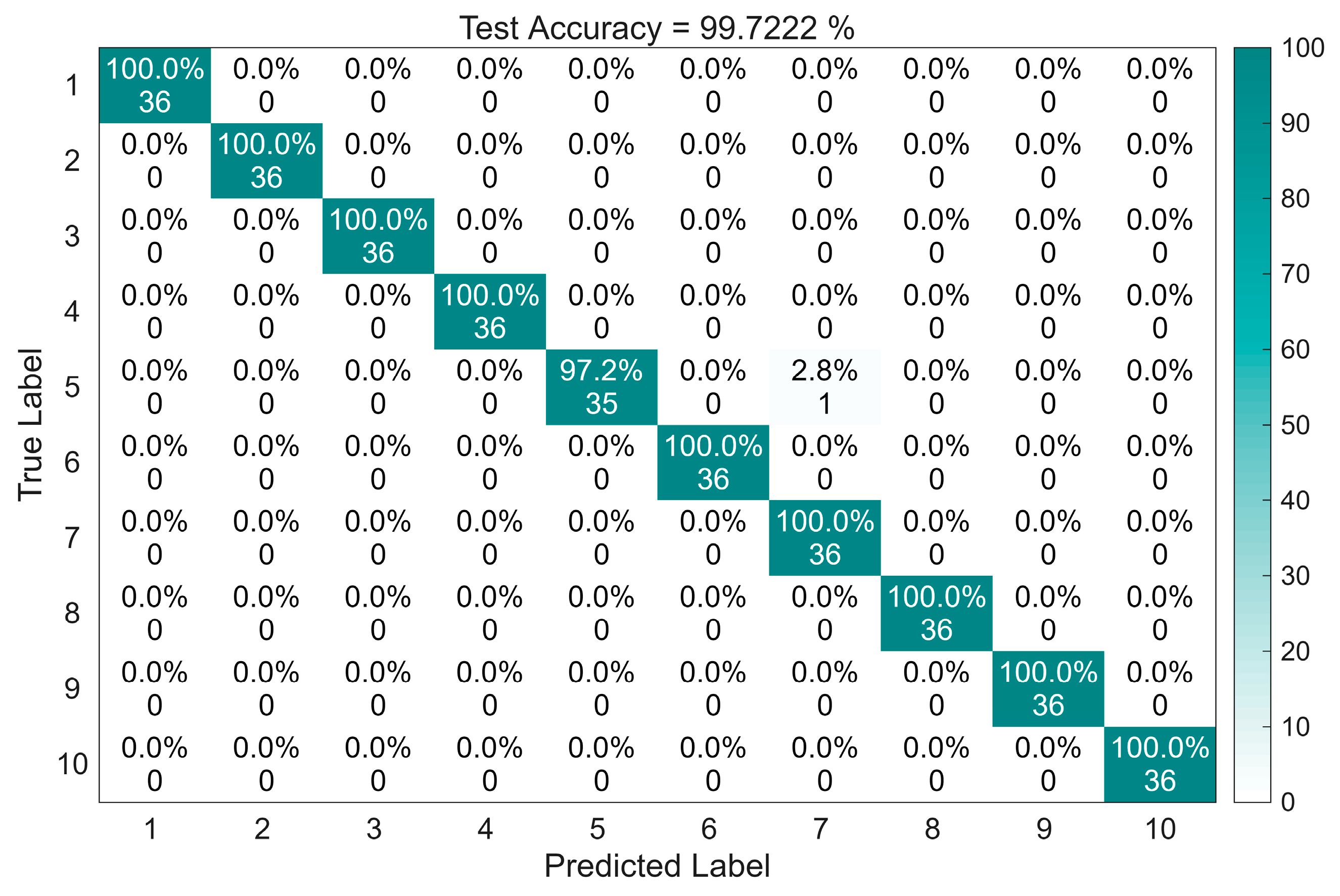
Figure 11 presents the confusion matrix of the training set, illustrating the prediction accuracy and misclassification among different categories. Figure 12 shows a comparison of predictions on the test sets. Figure 13 depicts the accuracy on the test set. After evaluation, the accuracy was 98.61% on the test set, indicating that it possesses strong predictive capability for practical applications.

Figure 11. Training set accuracy.

Figure 12. Test set prediction comparison.

Figure 13. Test set confusion matrix.

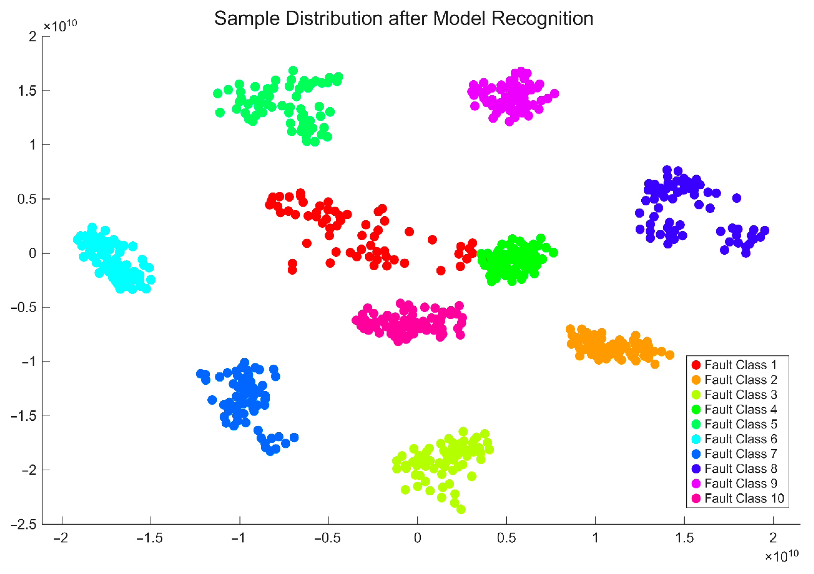
Finally, Figure 14 presents the t-SNE visualization of the proposed model, showing clear separability among fault classes. Distinct color-coded clusters indicate strong feature representation and effective discrimination, supporting the model’s robustness in classifying multiple fault types under variable operating conditions.

Figure 14. Feature distribution chart.

Extraction of Time-Domain Features and Construction of Frequency-Domain Images, this study prioritizes the use of multiscale permutation entropy (MPE) in the order domain as the fitness function for CPO-ICEEMDAN parameter optimization. Compared with sample entropy, information entropy, and envelope entropy, MPE is more robust to speed fluctuations and more sensitive to complexity changes induced by faults, thereby achieving higher discriminative power and stability in IMF selection and energy concentration. The CPO parameters were set as follows: number of iterations = 20, population size = 10, and ICEEMDAN iteration count = 100.

Table 5 summarizes the fault diagnosis performance of bearing signals based on envelope entropy, sample entropy, information entropy, and multiscale permutation entropy (MPE). Across the four evaluation metrics—MCC, Kappa, F1 score, and accuracy—the performance of the features shows a progressive improvement. Envelope entropy exhibits the lowest performance among the four metrics (MCC = 0.902, accuracy = 85.56%), indicating its limited ability to distinguish faults under complex variable-speed conditions. Sample entropy and information entropy achieve significant improvements across all metrics (MCC = 0.955 for sample entropy, MCC = 0.970 for information entropy), suggesting better capture of the non-stationary and nonlinear characteristics of the vibration signals.

Table 5. Comparison of Classification Performance of Different Entropy-Based Methods.

Label	MCC	Kappa	F1 Score	Accuracy
Envelope Entropy	0.902	0.904	92.85	85.56%
Sample Entropy	0.955	0.933	96.43	93.22%
Information Entropy	0.970	0.938	97.74	95.56%
Permutation Entropy	0.998	0.992	99.78	99.7222%

MPE, as a multiscale feature in the order domain, outperforms the other features in MCC (0.998), Kappa (0.992), F1 score (99.78), and accuracy (99.72%), demonstrating higher discriminative power and stability in IMF selection and energy concentration. It can more effectively handle speed fluctuations and fault complexity variations, fully validating the effectiveness of the proposed method.

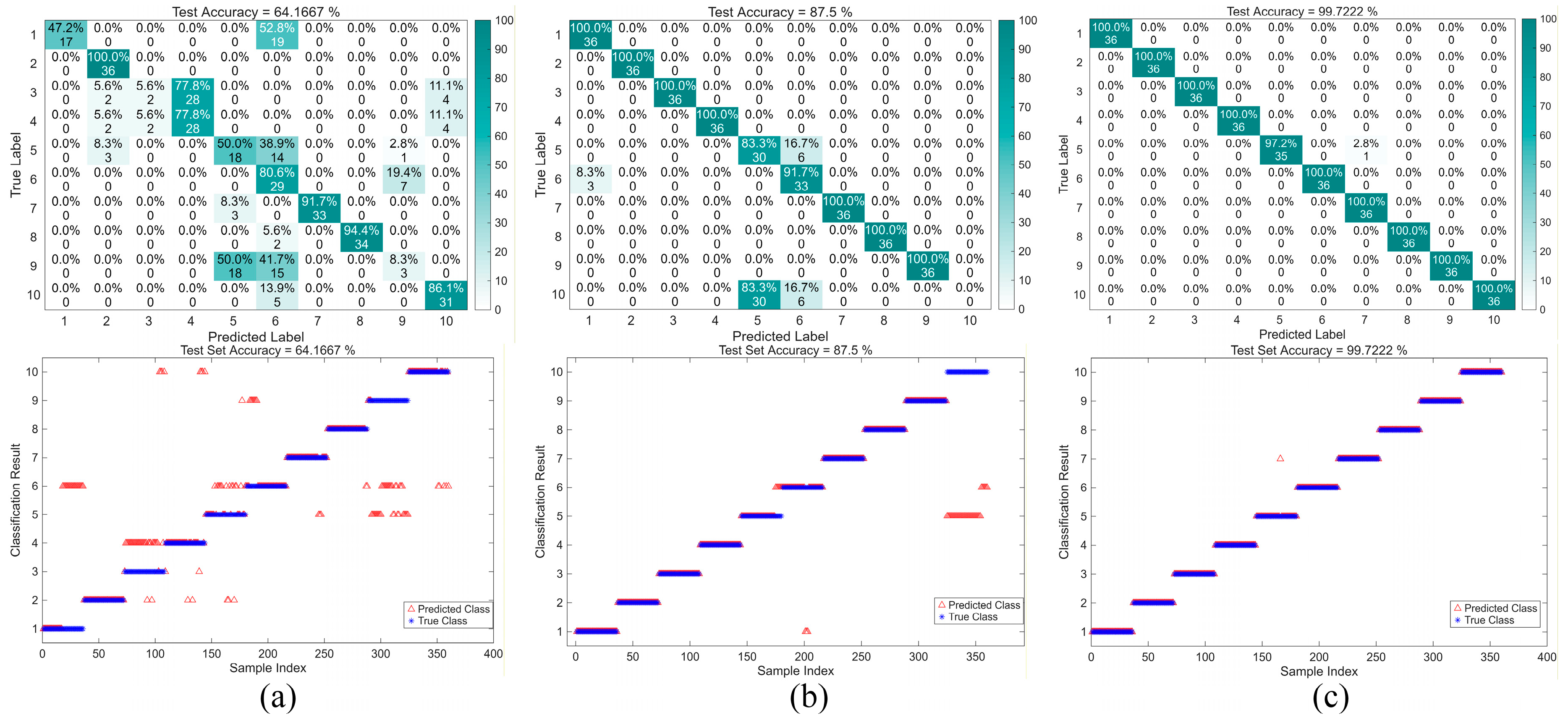
To further verify the effectiveness of the proposed approach in bearing fault diagnosis, three comparative experiments were designed: the baseline ResNet-18-GRU model; ICEEMDAN-ResNet-18-GRU, where vibration signals are decomposed using ICEEMDAN before being input to the model; and CPO-ICEEMDAN-ResNet-18-GRU, which employs CPO to optimize decomposition components and network parameters, achieving synergistic optimization of feature extraction and model performance. All models were trained and validated on the same training and test sets to compare the effects of different strategies on classification accuracy and robustness. Figure 15 shows the training curves for the three methods.

Figure 15. Training process curves of three methods: (a) Training set accuracy curves (b) Loss curves.

As shown in Figure 15, all three methods exhibit good convergence during training, but their convergence speeds and final performance differ significantly. The ResNet-18-GRU model converges relatively slowly in the early training stage, with noticeable fluctuations in training accuracy and a less smooth decrease in the loss value, indicating limitations in its feature extraction and temporal modeling capabilities. In contrast, the ICEEMDAN-ResNet-18-GRU model performs better during training. Its accuracy rises rapidly and stabilizes with fewer iterations, while the loss decreases more smoothly, demonstrating that ICEEMDAN decomposition effectively enhances the quality of input features, thereby improving training efficiency and stability. The CPO-ICEEMDAN-ResNet-18-GRU method achieves the best performance among the three. Its training accuracy consistently remains at the highest level, and the loss converges quickly to the minimum, exhibiting superior convergence speed and stability compared to the other two methods. This indicates that incorporating CPO optimization not only improves the effectiveness of feature decomposition but also enhances the model’s generalization capability and convergence performance. Figure 16a–c further present the test accuracy and confusion matrices of the three methods, where the baseline model shows more classification errors, the ICEEMDAN-enhanced model performs better, and the CPO-ICEEMDAN-ResNet-18-GRU achieves the most accurate and robust results. The accuracy comparison summarized in Table 6 also confirms this trend, with the proposed model achieving the highest test accuracy among the three methods.

Figure 16. Comparison of test set classification results for three methods: (a) ResNet-18-GRU (b) ICEEMDAN-ResNet-18-GRU (c) CPO-ICEEMDAN-ResNet-18-GRU.

Table 6. Accuracy under different models.

Model	ResNet18-GRU	ICEEMDAN-ResNet18-GRU	CPO-ICEEMDAN-ResNet18-GRU
Accuracy	64.1677%	87.5%	99.7222%

As shown in Figure 17, the classification accuracy on the test set differs significantly among the methods. The ResNet-18-GRU model achieves an overall accuracy of only 64.17%, with the confusion matrix showing noticeable cross-misclassifications and relatively low recognition rates for certain categories, indicating limitations in complex feature extraction and temporal information modeling. In contrast, the ICEEMDAN-ResNet-18-GRU model demonstrates a substantial improvement in classification performance. Its test accuracy reaches 87.5%, and most categories in the confusion matrix achieve near 100% recognition, with a significant reduction in misclassifications. This indicates that ICEEMDAN decomposition effectively enhances the time–frequency features of the input signal, thereby improving the model’s discriminative capability. The CPO-ICEEMDAN-ResNet-18-GRU model exhibits the best performance, achieving a test accuracy of 99.72% and nearly perfect classification, with predictions closely matching the true labels. This demonstrates that CPO optimization plays a crucial role in both feature decomposition and model parameter tuning, effectively enhancing the model’s robustness and generalization performance. In summary, the three methods show a progressive improvement in classification performance, validating the necessity and effectiveness of incorporating signal decomposition and optimization algorithms into traditional deep learning frameworks.

Figure 17. Feature distribution chart.

4.2.3. Comparison with Other Methods

To validate the effectiveness of the proposed method, DBO-SVM, DBN-LSSVM, MCNN, CNN-LSTM, and GRU-ResNet18 were employed as baseline models. Parameter settings and training were conducted under identical experimental conditions. Table 7 presents the key parameters and final classification accuracy for each model. Comparing the performance of these approaches clearly demonstrates the advantages and superiority of the proposed method.

Table 7. Comparison of Different Methods.

Model	Parameter Settings	Accuracy
DBO-SVM	Population size: 22, Iterations: 100	92.11%
DBN-LSSVM	Learning rate: 0.1, Hidden nodes: 30, Iterations: 2000	93.5%
MCNN	Training epochs: 30, Learning rate: 0.001, Learning rate decay factor: 0.01	95.22%
CNN-LSTM	Training epochs: 50, Learning rate: 0.001, Batch size: 64, Regularization: 0.0001	98.56%
GRU-ResNet18	Training epochs: 50, Learning rate: 0.0001, Batch size: 64, Regularization: 0.0001	99.72%

As shown in Table 7, the diagnostic performance of different methods under multi-condition variable-speed scenarios exhibits significant differences. The traditional DBO-SVM achieves an accuracy of 92.11% after parameter optimization, indicating a certain ability to recognize complex non-stationary signals, but its overall performance is limited by reliance on handcrafted features and insufficient generalization capability.

In contrast, DBN-LSSVM leverages a deep network structure to automatically extract features, increasing the accuracy to 93.5% and demonstrating the advantage of deep learning in feature representation. Further, the MCNN model enhances the expression of time–frequency features through its multi-channel convolutional structure, achieving an accuracy of 95.22% and showing greater robustness under complex operating conditions.

Building on this, the CNN-LSTM model combines convolutional feature extraction with sequence modeling, effectively capturing the temporal dependencies in variable-speed signals and achieving a significant accuracy improvement to 98.56%. Finally, the GRU-ResNet18 model, benefiting from ResNet’s deep residual structure for enhanced feature representation and GRU’s dynamic temporal modeling capability, attains the highest accuracy of 99.72% under complex multi-condition scenarios, clearly outperforming the other methods. These results indicate that the proposed method better adapts to the feature distribution of non-stationary vibration signals, demonstrating stronger robustness and generalization capability.

4.3. Validation Experiments Using a Public Bearing Dataset

Table 8 presents the experimental bearing data provided by the University of Ottawa [37,38], which consists of a motor, AC speed controller, drive shaft, and supporting bearings. As shown in Figure 17, the system consists of a motor, AC speed controller, drive shaft, and supporting bearings. Vibration signals were acquired using an ICP accelerometer, and rotational speed signals were synchronously recorded Via an incremental encoder (EPC 775). The sampling frequency was 200 kHz, with a single acquisition lasting 10 s, and each state was repeated three times. Figure 18 shows the time-domain plot.

Table 8. University of Ottawa bearing data information.

Bearing Health Conditions	Speed Varying Conditions
	Increasing Speed (Hz)	Decreasing Speed (Hz)	Increasing then Decreasing Speed (Hz)	Decreasing then Increasing Speed (Hz)
Healthy	H-A-1 (14.1–23.8)	H-B-1 (28.9–13.7)	H-C-1 (14.7–25.3–21.0)	H-D-1 (24.2–14.8–20.6)
	H-A-2 (14.1–29.0)	H-B-2 (25.7–11.6)	H-C-2 (14.4–24.0–18.7)	H-D-2 (24.6–14.0–18.6)
	H-A-3 (15.2–26.7)	H-B-3 (28.6–13.9)	H-C-3 (15.4–24.0–18.7)	H-D-3 (26.0–16.9–23.2)
Inner race fault	I-A-1 (15.2–26.7)	I-B-1 (24.3–9.9)	I-C-1 (15.1–24.4–18.7)	I-D-1 (25.3–14.8–19.4)
	I-A-2 (13.0–25.7)	I-B-2 (25.1–13.1)	I-C-2 (14.1–23.5–18.0)	I-D-2 (25.3–15.1–19.8)
	I-A-3 (13.5–28.5)	I-B-3 (25.8–12.0)	I-C-3 (14.8–21.7–13.6)	I-D-3 (23.1–15.7–23.6)
Outer race fault	O-A-1 (14.8–27.1)	O-B-1 (24.9–9.8)	O-C-1 (14.0–21.7–14.5)	O-D-1 (26.0–18.9–24.5)
	O-A-2 (12.9–23.0)	O-B-2 (24.7–10.2)	O-C-2 (14.0–24.5–19.8)	O-D-2 (25.2–14.6–19.5
	O-A-3 (13.3–26.3)	O-B-3 (25.4–10.3)	O-C-3 (14.2–23.4–17.6)	O-D-3 (25.5–15.0–19.6)
Ball fault	B-A-1 (14.3–24.6)	B-B-1 (27.0–11.5)	B-C-1 (16.9–23.7–15.7)	B-D-1 (22.0–14.6–20.9)
	B-A-2 (13.1–28.4)	B-B-2 (25.4–10.0)	B-C-2 (14.3–23.4–17.8)	B-D-2 (23.5–15.4–22.1)
	B-A-3 (13.4–28.0)	B-B-3 (30.6–15.1)	B-C-3 (15.2–22.1–14.6)	B-D-3 (25.5–17.4–23.9)
Compound fault	C-A-1 (13.3–27.8)	C-B-1 (26.8–11.4)	C-C-1 (15.1–21.1–12.3)	C-D-1 (24.3–15.5–21.5)
	C-A-2 (13.2–28.5)	C-B-2 (27.4–12.0)	C-C-2 (14.9–21.6–13.4)	C-D-2 (23.9–16.1–22.9)
	C-A-3 (13.5–28.3)	C-B-3 (27.9–12.5)	C-C-3 (15.1–22.7–15.8)	C-D-3 (23.7–16.5–23.8)

Figure 18. Time domain waveform of data A.

This subsection of the dataset covers five bearing conditions and four speed variation patterns yielding a total of 36 groups. For this study, 10 representative groups (BA1, BA2, CA1, CA2, HA1, HA2, IA1, IA2, OA1, OA2) were selected for analysis, with Channel_1 vibration signals used for each group. These signals exhibit significant non-stationarity and complex characteristics, providing an effective test for evaluating the robustness, stability, and generalization capability of the proposed multimodal fault diagnosis method under various fault types and variable-speed conditions.

Figure 19 shows that the test set achieves an accuracy of 98.61%, with only a few misclassifications, indicating the method’s reliable performance under multi-class and variable-speed conditions. Figure 20 further illustrates that the predicted labels closely align with the true labels, demonstrating strong generalization ability. In Figure 21, the features projected into a reduced-dimensional space form well-separated clusters, highlighting the effectiveness of the feature extraction and discriminative capability. Overall, despite the non-stationary and complex nature of the data, the proposed multimodal approach achieves stable and accurate fault identification, confirming its robustness and generalization performance.

Figure 19. Test set confusion matrix.

Figure 20. Test set prediction comparison.

Figure 21. Feature distribution chart.

5. Conclusions

To address the challenges of non-stationarity, strong nonlinearity, ambiguous time-frequency characteristics, and overlapping fault features in bearings under variable-speed hybrid conditions, this paper proposes a bearing fault diagnosis method based on CPO-optimized ICEEMDAN decomposition and dual-modal time-series and image deep feature fusion. By adaptively optimizing ICEEMDAN parameters with the CPO algorithm, the method achieves effective signal decomposition and fault feature enhancement. Combined with time-domain features and time-frequency images, the dual-modal inputs improve multidimensional feature representation. The dual-branch deep learning model, comprising a GRU-based time-series branch and an SE-ResNet18 image branch, enables multimodal feature extraction and fused classification. Experimental results on a self-collected dataset and the publicly available Ottawa variable-speed bearing dataset demonstrate that the proposed method achieves high-accuracy fault identification with strong robustness and generalization capability, validating its effectiveness for intelligent bearing fault diagnosis under complex variable-speed hybrid conditions and providing a reference for reliable industrial equipment operation.

Future work may focus on further optimizing signal preprocessing and feature extraction strategies to accommodate more complex operating conditions, introducing lightweight models and online learning mechanisms for real-time intelligent diagnosis, and extending the method to other types of rotating machinery to enhance the applicability and reliability of intelligent fault diagnosis systems.

References

- Peng, B.; Bi, Y.; Xue, B.; Zhang, M.; Wan, S. A survey on fault diagnosis of rolling bearings. Algorithms 2022, 15, 347. [Google Scholar] [CrossRef]
- Cerrada, M.; Sánchez, R.V.; Li, C.; Pacheco, F.; Cabrera, D.; de Oliveira, J.V.; Vásquez, R.E. A review on data-driven fault severity assessment in rolling bearings. Mech. Syst. Signal Process. 2018, 99, 169–196. [Google Scholar] [CrossRef]
- He, M.; He, D. Deep learning based approach for bearing fault diagnosis. IEEE Trans. Ind. Appl. 2017, 53, 3057–3065. [Google Scholar] [CrossRef]
- Sun, S.; Xia, X.; Zhou, H. Bearing fault diagnosis under time-varying speeds with limited samples using frequency temporal series graph and graph generative classified adversarial networks. Neurocomputing 2025, 647, 130613. [Google Scholar] [CrossRef]
- Chen, Y.; Yue, J.; Liu, Z.; Chen, J. A semi-supervised wise-attention weighted prototype network for rolling bearing fault diagnosis under noisy and limited labeled data conditions. Neurocomputing 2025, 647, 130563. [Google Scholar] [CrossRef]
- Li, X.; Wang, J.; Wang, J.; Wang, J.; Liu, J.; Chen, J.; Yu, X. Research on CNC Machine Tool Spindle Fault Diagnosis Method Based on Deep Residual Shrinkage Network with Dynamic Convolution and Selective Kernel Attention Model. Algorithms 2025, 18, 569. [Google Scholar] [CrossRef]
- Song, B.; Liu, Y.; Fang, J.; Liu, W.; Zhong, M.; Liu, X. An optimized CNN-BiLSTM network for bearing fault diagnosis under multiple working conditions with limited training samples. Neurocomputing 2024, 574, 127284. [Google Scholar] [CrossRef]
- Zhang, L.; Zhang, Y.; Li, G. Fault-diagnosis method for rotating machinery based on SVMD entropy and machine learning. Algorithms 2023, 16, 304. [Google Scholar] [CrossRef]
- Chen, Y.; Zhang, T.; Zhao, W.; Luo, Z.; Sun, K. Fault diagnosis of rolling bearing using multiscale amplitude-aware permutation entropy and random forest. Algorithms 2019, 12, 184. [Google Scholar] [CrossRef]
- Bang, J.; Di Marco, P.; Shin, H.; Park, P. Deep Transfer Learning-Based Fault Diagnosis Using Wavelet Transform for Limited Data. Appl. Sci. 2022, 12, 7450. [Google Scholar] [CrossRef]
- Meng, D.; Wang, H.; Yang, S.; Lv, Z.; Hu, Z.; Wang, Z. Fault Analysis of Wind Power Rolling Bearing Based on EMD Feature Extraction. Comput. Model. Eng. Sci. 2022, 130, 543–558. [Google Scholar] [CrossRef]
- Peng, Y.H. De-Noising by Modified Soft-Thresholding. In Proceedings of the 2000 IEEE Asia-Pacific Conference on Circuits and Systems. Electronic Communication Systems, Tianjin, China, 4–6 December 2000; Volume 3. [Google Scholar]
- Chen, Y.; Wang, Y.; Ma, G.; Wang, Y.; Sun, Y.; He, Y. Weak fault feature extraction of rolling bearings based on improved ensemble noise-reconstructed EMD and adaptive threshold denoising. Mech. Syst. Signal Process. 2022, 171, 108834. [Google Scholar] [CrossRef]
- Wu, Z.; Huang, N.E. Ensemble empirical mode decomposition: A noise-assisted data analysis method. Adv. Adapt. Data Anal. 2009, 1, 1–41. [Google Scholar] [CrossRef]
- Puntambekar, R.; Vyas, P.; Thakkar, A.; Patel, D. A survey of machine learning and deep learning methods for vibration-based Bearing fault diagnosis: The need, challenges, and potential future research Directions. Neurocomputing 2025, 659, 131628. [Google Scholar] [CrossRef]
- Colominas, M.A.; Schlotthauer, G.; Torres, M.E. Improved complete ensemble EMD: A suitable tool for biomedical signal processing. Biomed. Signal Process. Control 2014, 14, 19–29. [Google Scholar] [CrossRef]
- Lei, Y.; Liu, Z.; Ouazri, J.; Lin, J. A fault diagnosis method of rolling element bearings based on CEEMDAN. Proc. Inst. Mech. Eng. Part C J. Mech. Eng. Sci. 2017, 231, 1804–1815. [Google Scholar] [CrossRef]
- Li, T.; Yu, M.; Ma, T.; Du, Y.; Dou, S. Fault Diagnosis of Printing Machine Bearings based on Improved Empirical Mode Decomposition and DBO-SVM. J. Imaging Sci. Technol. 2025, 69, 1–14. [Google Scholar] [CrossRef]
- Hou, S.Z.; Guo, W.; Wang, Z.Q.; Liu, Y.T. Deep-learning-based fault type identification using modified CEEMDAN and image augmentation in distribution power grid. IEEE Sens. J. 2021, 22, 1583–1596. [Google Scholar] [CrossRef]
- Lv, Z.; Luo, J.; Li, L.; Jia, X.; Zhou, J.; Wang, Z. Weak fault feature extraction method for RV reducer based on CPO-MNAD and LCPSO-BP neural network. IEEE Sens. J. 2025, 25, 26383–26397. [Google Scholar] [CrossRef]
- Chen, S.; Shi, H.; Luo, L.; Qiu, H.; Chang, L. A Hybrid Fault Diagnosis Framework for High-Voltage Circuit Breakers: NRBO-Optimized ICEEMDAN and CPO-Enhanced CNN-SVM. IEEE Access 2025, 13, 175821–175846. [Google Scholar] [CrossRef]
- Chen, X.; Yang, R.; Xue, Y.; Huang, M.; Ferrero, R.; Wang, Z. Deep transfer learning for bearing fault diagnosis: A systematic review since 2016. IEEE Trans. Instrum. Meas. 2023, 72, 1–21. [Google Scholar] [CrossRef]
- Li, Z.; Liu, F.; Yang, W.; Peng, S.; Zhou, J. A survey of convolutional neural networks: Analysis, applications, and prospects. IEEE Trans. Neural Netw. Learn. Syst. 2021, 33, 6999–7019. [Google Scholar] [CrossRef] [PubMed]
- He, K.; Gkioxari, G.; Dollár, P.; Girshick, R. Mask R-CNN. In Proceedings of the IEEE International Conference on Computer Vision, Venice, Italy, 22–29 October 2017; pp. 2961–2969. [Google Scholar]
- Chua, L.O. CNN: A Paradigm for Complexity; World Scientific: Singapore, 1998. [Google Scholar]
- Kattenborn, T.; Leitloff, J.; Schiefer, F.; Hinz, S. Review on Convolutional Neural Networks (CNN) in vegetation remote sensing. ISPRS J. Photogramm. Remote Sens. 2021, 173, 24–49. [Google Scholar] [CrossRef]
- Liang, H.; Zhao, X. Rolling bearing fault diagnosis based on one-dimensional dilated convolution network with residual connection. IEEE Access 2021, 9, 31078–31091. [Google Scholar] [CrossRef]
- Luo, Z.; Pan, S.; Dong, X.; Zhang, X. Interpretable quadratic convolutional residual neural network for bearing fault diagnosis. J. Braz. Soc. Mech. Sci. Eng. 2025, 47, 158. [Google Scholar] [CrossRef]
- Li, Y.; Gu, X.; Wei, Y. A Deep Learning-Based Method for Bearing Fault Diagnosis with Few-Shot Learning. Sensors 2024, 24, 7516. [Google Scholar] [CrossRef]
- Huang, T.; Zhang, Q.; Tang, X.; Zhao, S.; Lu, X. A novel fault diagnosis method based on CNN and LSTM and its application in fault diagnosis for complex systems. Artif. Intell. Rev. 2022, 55, 1289–1315. [Google Scholar] [CrossRef]
- Lei, X.; Sui, Z. Intelligent fault detection of high voltage line based on the Faster R-CNN. Measurement 2019, 138, 379–385. [Google Scholar] [CrossRef]
- Zaman, W.; Siddique, M.F.; Khan, S.U.; Kim, J.-M. A new dual-input CNN for multimodal fault classification using acoustic emission and vibration signals. Eng. Fail. Anal. 2025, 179, 109787. [Google Scholar] [CrossRef]
- Chen, X.; Zhang, B.; Gao, D. Bearing fault diagnosis base on multi-scale CNN and LSTM model. J. Intell. Manuf. 2021, 32, 971–987. [Google Scholar] [CrossRef]
- Wang, X.; Mao, D.; Li, X. Bearing fault diagnosis based on vibro-acoustic data fusion and 1D-CNN network. Measurement 2021, 173, 108518. [Google Scholar] [CrossRef]
- Han, K.; Wang, W.; Guo, J. Research on a Bearing Fault Diagnosis Method Based on a CNN-LSTM-GRU Model. Machines 2024, 12, 927. [Google Scholar] [CrossRef]
- Siddique, M.F.; Saleem, F.; Umar, M.; Kim, C.H.; Kim, J.-M. A hybrid deep learning approach for bearing fault diagnosis using continuous wavelet transform and attention-enhanced spatiotemporal feature extraction. Sensors 2025, 25, 2712. [Google Scholar] [CrossRef] [PubMed]
- Huang, H.; Baddour, N. Bearing vibration data collected under time-varying rotational speed conditions. Data Brief 2018, 21, 1745–1749. [Google Scholar] [CrossRef] [PubMed]
- Li, S.; Peng, Y.; Shen, Y.; Zhao, S.; Shao, H.; Bin, G.; Guo, Y.; Yang, X.; Fan, C. Rolling bearing fault diagnosis under data imbalance and variable speed based on adaptive clustering weighted oversampling. Reliab. Eng. Syst. Saf. 2024, 244, 109938. [Google Scholar] [CrossRef]
Disclaimer/Publisher’s Note: The statements, opinions and data contained in all publications are solely those of the individual author(s) and contributor(s) and not of MDPI and/or the editor(s). MDPI and/or the editor(s) disclaim responsibility for any injury to people or property resulting from any ideas, methods, instructions or products referred to in the content. |
© 2025 by the authors. Licensee MDPI, Basel, Switzerland. This article is an open access article distributed under the terms and conditions of the Creative Commons Attribution (CC BY) license (https://creativecommons.org/licenses/by/4.0/).