A Multi-Surrogate Assisted Multi-Tasking Optimization Algorithm for High-Dimensional Expensive Problems

Abstract

Surrogate-assisted evolutionary algorithms (SAEAs) are widely used in the field of high-dimensional expensive optimization. However, real-world problems are usually complex and characterized by a variety of features. Therefore, it is very challenging to choose the most appropriate surrogate. It has been shown that multiple surrogates can characterize the fitness landscape more accurately than a single surrogate. In this work, a multi-surrogate-assisted multi-tasking optimization algorithm (MSAMT) is proposed that solves high-dimensional problems by simultaneously optimizing multiple surrogates as related tasks using the generalized multi-factorial evolutionary algorithm. In the MSAMT, all exactly evaluated samples are initially grouped to form a collection of clusters. Subsequently, the search space can be divided into several areas based on the clusters, and surrogates are constructed in each region that are capable of completely describing the entire fitness landscape as a way to improve the exploration capability of the algorithm. Near the current optimal solution, a novel ensemble surrogate is adopted to achieve local search in speeding up the convergence process. In the framework of a multi-tasking optimization algorithm, several surrogates are optimized simultaneously as related tasks. As a result, several optimal solutions spread throughout disjoint regions can be found for real function evaluation. Fourteen 10- to 100-dimensional test functions and a spatial truss design problem were used to compare the proposed approach with several recently proposed SAEAs. The results show that the proposed MSAMT performs better than the comparison algorithms in most test functions and real engineering problems.

1. Introduction

Evolutionary algorithms (EAs), such as genetic algorithms (GAs) [1], differential evolution (DE) [2], and particle swarm optimization (PSO) [3], have been successfully utilized in various practical engineering problems, such as the design of aircraft wings [4], robotics [5], wireless networks [6], and the optimization of vehicle technology trajectory [7,8]. However, the utilization of EAs to address optimization problems requires hundreds of expensive exact fitness evaluations (FEs) to achieve an acceptable solution, which severely hinders their application in practical engineering problems. To solve this problem, SAEAs have been proposed. SAEAs are a class of techniques that combine EAs with surrogate models, which build inexpensive surrogate models for predicting the fitness values of candidate solutions as a replacement for FEs in the EAs. In recent years, the use of SAEAs for optimization problems has received increasing attention because the computational cost of constructing surrogates and predicting fitness values is less than FEs.

Model management strategy is crucial for SAEAs, which select some new samples for exact FEs and use them in the reconstruction of the surrogate model [9]. Currently developed model management strategies are mainly categorized as generation-based and individual-based, where the former selects all samples by generation for accurate FEs and the latter selects promising individuals for real evaluation. Both strategies have been shown to be effective, but in general, individual-based criteria are more flexible than generation-based criteria [10,11]. There are usually two criteria for selecting promising individuals. The first is the performance-based criterion that chooses the individual with the best fitness value for accurate evaluation to effectively enhance the performance of the surrogate and facilitate the exploitation of the currently promising area [12]. The second category is the uncertainty-based criterion, which can enhance exploration by selecting the most uncertain individual for accurate evaluation [13]. It has been shown [14] that using only one infill criterion may lead to early convergence or falling into a local optimum. Therefore, this paper selects the optimal or average individual for real function evaluation.

The current SAEAs can be classified into two principal categories. The first category is the single-layer SAEAs, which do not have hierarchically organized components and usually use only one model, i.e., a local or global surrogate, to assist one evolutionary algorithm. Li et al. [15] presented a fast algorithm using the global radial basis function (RBF) to assist PSO, in which they combined the performance-based criterion with a new criterion that considered the distance and fitness value concurrently, boosting the efficiency of the algorithm. Li et al. [16] also developed a surrogate-assisted multi-swarm optimization technique that alternately carries out teaching-learning-based optimization (TLBO) to enhance exploration and PSO to accelerate convergence. Global surrogates can summarize the overall fitness landscape. Nourian et al. [17] combined graphical neural networks (GNNs) and PSO for optimal design of truss structures. However, generally speaking, a large number of exactly evaluated samples are required to build highly accurate global surrogates when solving large-scale expensive optimization problems, which can make it difficult for algorithms to balance between high accuracy and low time consumption. Therefore, local surrogates are commonly used to increase the accuracy by capturing the regional characteristics of the fitness landscape. Cai et al. [18] presented a search technique based on trust region, which is to establish a local RBF model in the trust region surrounding the optimal population, thereby boosting the optimization efficiency. Pan et al. [19] used neighbor samples to train a local RBF model with higher accuracy to assist the TLBO and DE alternately and proposed a new prescreening criterion.

The second type is known as the hierarchical SAEAs, where multiple models are used to assist different EAs. The fine local surrogate is utilized to depict the specifics of the fitness landscape, while the rough global surrogate is utilized to mitigate the impact of local optima. Sun et al. [20] developed a hierarchical surrogate that uses both local and global models to assist PSO in directing the swarm towards the global optima. Wang et al. [21] developed the use of global RBF and local Kriging to assist DE for high-dimensional expensive problems. Kůdela et al. [22] integrated global RBF and a new Lipschitz-based-surrogate-assisted global optimization procedure with local optimization based on a local RBF model. Hierarchical SAEAs may increase the computational overhead compared to single-layer SAEAs, which can provide a solution in a shorter amount of time. However, for high-dimensional multimodal problems, hierarchical SAEAs are preferred. Hierarchical SAEAs can first identify promising regions in the global search phase and then explore more deeply in local regions, which is very beneficial for a comprehensive search of the decision space.

The reliability of SAEAs is mainly influenced by the surrogate and the evolutionary algorithm. With an increase in problem dimensions, the single surrogate easily causes the algorithm to be trapped in local optima. Meanwhile, the fixed surrogate makes it quite difficult to accurately describe different optimization problems. Therefore, to address this issue, the ensemble of surrogates is widely used in SAEAs [23,24]. Ren et al. [25] developed a hybrid algorithm that first carries out a series of global searches, then takes turns with global and local searches and employs social learning particle swarm optimization (SL-PSO) and DE for global searches assisted by a surrogate ensemble and local searches assisted by RBF, respectively. Guo et al. [13] replaced the time-consuming Gaussian processes with a heterogeneous integration composed of models with different input characteristics, which improves the diversity and reliability of the surrogate. Moreover, research on adaptive surrogate model selection techniques has also received more and more attention. Li et al. [26] adaptively selected one from an RBF or an ensemble model to facilitate PSO according to standard deviation. Liu et al. [27] introduced a decision space partition-based SAEA when addressing expensive optimization problems, which divides the space into several disjoint regions by the k-means clustering technique and establishes an RBF model on each region to assist PSO in global search, and an adaptive surrogate is utilized to assist local exploitation. Zhang et al. [28] designed a hierarchical surrogate framework that adopts RBF-assisted TLBO to locate promising regions and the dynamic surrogate-assisted DE to precisely determine the global optimal solution. The evolutionary algorithm is also a key component of SAEAs. When faced with a complex problem, a single EA may induce the optimization process to follow a similar trajectory and become trapped into local optima [29]. As a result, several SAEAs use different EAs at the same time. In addition, some SAEAs using the multi-task evolutionary algorithm have been developed. Multi-task optimization (MTO) is a method that can process several optimization tasks simultaneously, and it can promote the overall task solving progress through the data transfer between different tasks. Liao et al. [30] introduced a multi-tasking algorithm design framework that uses the generalized multi-factorial evolutionary algorithm (G-MFEA) to assist global and local surrogates simultaneously in addressing expensive optimization problems. Yang et al. [31] took a global Kriging or a local RBF model as the assistant task at different stages and then used the MFEA to optimize the assistant task and the target task simultaneously.

In addition, multi-agent systems using the partition idea are also effective in preventing algorithms from falling into local optima. Intelligent agents evolve in the decomposed dimensional space to find local suboptimal solutions, and the global optimum is determined in the dynamic interaction of intelligent agents. Akopov et al. [32] proposed a multi-agent genetic algorithm for multi-objective optimization, in which global optimization is achieved in the process of coordinating intelligent agents and significantly reduces the number of true function evaluations. Zhong et al. [33] proposed a multi-agent genetic algorithm that fixes all agents in a lattice environment and then uses the competition or cooperation of these agents to find the global optimum solution. Table 1 summarizes the important algorithms, including EAs and SAEAs.

Table 1. Currently important algorithms, including EAs and SAEAs.

Algorithm	Author, References	Surrogate Models	Evolutionary Algorithms	Year
MFEA	Gupta et al. [34]	×	MFEA	2016
G-MFEA	Ding et al. [35]	×	GMFEA	2017
FSAPSO	Li et al. [15]	RBF	PSO	2020
BiS-SAHA	Ren et al. [25]	RBF	SL-PSO, DE	2021
GL-SADE	Wang et al. [21]	RBF, Kriging	DE	2023
LSADE	Kůdela et al. [22]	RBF, Lipschitz	DE	2023
DSP-SAEA	Liu et al. [27]	RBF, Kriging, and polynomial regression (PR)	PSO	2023
SAMTO	Yang et al. [31]	Kriging, RBF	MFEA	2023
HSAOA	Zhang et al. [28]	RBF, PRS, and SVR	TLBO, DE	2024

Inspired by the above surrogate-assisted optimization techniques, this study presents a novel multi-surrogate-assisted multi-tasking optimization algorithm (MSAMT) for large-scale optimization problems. The algorithm design first divides the entire goal space into different regions and constructs the corresponding RBF model for each region to support the global exploration. Then, a novel dynamic ensemble of surrogates is used to build surrogate-assisted local exploitation with high reliability near the current optimal solution. Finally, the G-MFEA is used to assist multiple surrogates in searching each subregion and the space around the current optimal solution. The following are the innovations and major contributions of the proposed method:

• Under the framework of the G-MFEA, a space partition strategy is used to introduce multiple surrogate models as optimization tasks, and global and local searches are carried out simultaneously so that the algorithm can achieve good exploration and considerably reduce the chance of falling into local optima.
• A novel dynamic ensemble of surrogates is proposed. In this adaptive strategy, a single surrogate or an ensemble of two surrogates or three surrogates is selected as a local model from the base model pool (including RBF, polynomial response surface (PRS), and support vector regression (SVR)) according to the error index, thus accelerating the convergence.
• Experimental results indicate that the proposed algorithm has better performance than the competition algorithm in most of the test functions and a truss design problem, resulting in better results and faster convergence processes.

The rest of this paper is structured as follows: Section 2 briefly reviews the information on the surrogate models (RBF, PRS, SVR, and the ensemble of surrogates) and the MFEA, and introduces the details of the MSAMT. The performance of the proposed algorithm is evaluated by extensive empirical studies in Section 3. Lastly, Section 4 concludes this work.

2. Materials and Methods

This section first introduces the surrogate models (SVR, RBF, PRS, and the unified ensemble of surrogates) used in this work, followed by a brief description of the MFEA.

2.1. Polynomial Response Surface

Box and Wilson first proposed [36] the PRS model, which is one of the most commonly used surrogates. The most widely utilized is the second-order polynomial function, because overfitting occurs easily when the order exceeds 3. The second-order PRS can be represented as follows:

$$\widehat{y}\left(\mathit{x}\right)={\beta }_0+\sum _{i=1}^m{\beta }_i{x}_i+\sum _{i=1}^m{\beta }_{ii}{x}_i^2+\sum _{i=1}^{m-1}\sum _{j=i+1}^m{\beta }_{ij}{x}_i{x}_j$$

(1)

where $\widehat{y}\left(x\right)$ is the predicted value of the surrogate, $m$ denotes the number of input variables, and $\beta =\left[{\beta }_0, {\beta }_i, {\beta }_{ii}, {\beta }_{ij}\right]$ represents the coefficient that needs to be determined.

PRS has the advantages of strong interpretability, simple computation, high efficiency, and good noise filtering, which make it effective for low-dimensional nonlinear problems. However, with the increase in problem dimensions, the accuracy of PRS is relatively low.

2.2. Radial Basis Function

The RBF model, which was first developed by Hardy [37], can be used to approximate irregular terrain. The interpolation form of RBF is as follows:

$$\widehat{y}\left(\mathit{x}\right)=\sum _{i=1}^n{\omega }_i{\phi }_i\left(‖\mathit{x}-x_i‖\right)$$

(2)

where $n$ represents the sample size, ${\phi }_i\left(·\right)$ represents the ith basis function, $\omega =\left[{\omega }_1, {\omega }_2, \cdots , {\omega }_n\right]$ denotes the weight coefficient, and $‖·‖$ represents the Euclidean distance between two samples. It is important to note that there are multiple kinds of basis functions, including thin plate splines, linear splines, cubic splines, and so on.

2.3. Support Vector Regression

The SVR surrogate model is given as follows:

$$\widehat{y}\left(\mathit{x}\right)=\mu +\sum _{i=1}^n{\omega }_i\psi \left(\mathit{x},x_i\right)$$

(3)

Faced with a linear function approximation, SVR can be recalculated as follows:

$$\widehat{y}\left(\mathit{x}\right)=\mu +⟨\mathit{\omega },\mathit{x}⟩$$

(4)

where $\mu$ is the threshold and $⟨·,·⟩$ represents the dot product. Find the weights that minimize the margin $\epsilon$ corresponding to solving the optimization problem and introduce slack variables ${\xi }_i$ and ${\xi }_i^{\mathrm{*}}$ to keep $\widehat{y}\left(x\right)$ as flat as possible:

$$\begin{gathered} \mathrm{m}\mathrm{i}\mathrm{n}{\displaystyle \frac{1}{2}}{‖\mathit{\omega }‖}^2+\gamma \sum _{i=1}^n\left({\xi }_i+{\xi }_i^{*}\right) \\ \mathrm{s}.\mathrm{t}.\left\{\begin{array}{c}{y}_i-⟨\mathit{\omega },x_i⟩-\mu \le \epsilon +{\xi }_i, i=1,2,\cdots ,n\hfill \\ ⟨\mathit{\omega },x_i⟩+\mu -y_i\le \epsilon +{\xi }_i^{*}, i=1,2,\cdots ,n\hfill \\ {\xi }_i,{\xi }_i^{*}\ge 0, i=1,2,\cdots ,n\hfill \end{array}\right. \end{gathered}$$

(5)

where $\gamma$ represents a regularization parameter that controls the trade-off between the complexity of the model and the level at which errors are allowed to exceed $\epsilon$. The following formula can be used to obtain the weight coefficient:

$$\mathit{\omega }=\sum _{i=1}^n\left({\alpha }_i-{\alpha }_i^{*}\right)x_i$$

(6)

where ${\alpha }_i$ and ${\alpha }_i^{*}$ are the Lagrange multipliers. The SVR model obtained by inserting Equation (6) into Equation (4) is as follows:

$$\widehat{y}\left(\mathit{x}\right)=\mu +\sum _{i=1}^n\left({\alpha }_i-{\alpha }_i^{*}\right)⟨x_i,\mathit{x}⟩$$

(7)

For nonlinear approximation, the kernel function can be used to replace the dot product of the input vectors to obtain the nonlinear transformation, and the resulting SVR model is expressed as follows:

$$\widehat{y}\left(\mathit{x}\right)=\mu +\sum _{i=1}^n\left({\alpha }_i-{\alpha }_i^{*}\right)k\left(x_i,\mathit{x}\right)$$

(8)

2.4. Dynamic Ensemble of Surrogates

Generally speaking, there is no single surrogate that outperforms other surrogates in all kinds of problems. Therefore, the ensemble surrogate, which consists of several component surrogates that can fully utilize the benefits of each surrogate, has been widely used. The prediction of the ensemble surrogate is obtained through weighting the predicted value of multiple surrogates, so the approximate fitness of the samples can be determined by the following:

$${\widehat{y}}_{ens}\left(\mathit{x}\right)=\sum _{i=1}^{N_{ens}}{\omega }_i\left(\mathit{x}\right){\widehat{y}}_i\left(\mathit{x}\right)$$

(9)

where ${\widehat{y}}_{ens}\left(\mathit{x}\right)$ is the prediction of the ensemble of surrogates, ${\widehat{y}}_i\left(\mathit{x}\right)$ denotes the prediction of the ith surrogate, and $N_{ens}$ is the number of surrogates, ${\omega }_i\left(\mathit{x}\right)$ is the weight factor of the ith surrogate, and ${\omega }_i\left(\mathit{x}\right)$ needs to meet the formula ${\sum }_{i=1}^{N_{ens}}{\omega }_i\left(\mathit{x}\right)=1$.

According to the characteristics of weight coefficients, the existing methods for ensemble modeling can be classified into global measures-based, local measures-based, and mixed measures-based. The weight coefficient in global measures is a constant calculated according to the global error of each surrogate, while the weight coefficient in local measures is influenced by the location of the prediction sample. The former ignores the difference in fitting accuracy of the model in local areas, while the accuracy of the latter may decline away from the sample points. Mixed measures-based combines the advantages of the two, taking into account the regions near and away from the samples. On the basis of the existing methods, Zhang et al. [38] suggested a new unified ensemble of surrogates (UES), which integrates global and local measures, and the weight coefficients are determined according to the position of the predicted sample within the entire decision space as follows:

$${\omega }_i\left(\mathit{x}\right)={\displaystyle \frac{{\omega }_i^G\left(\mathit{x}\right)\lambda \left(\mathit{x}\right)+{\omega }_i^L\left(\mathit{x}\right)\left(1-\lambda \left(\mathit{x}\right)\right)}{{\sum }_{j=1}^{N_{ens}}\left[{\omega }_j^G\left(\mathit{x}\right)\lambda \left(\mathit{x}\right)+{\omega }_j^L\left(\mathit{x}\right)\left(1-\lambda \left(\mathit{x}\right)\right)\right]}}$$

(10)

where ${\omega }_i^G\left(\mathit{x}\right)$ and ${\omega }_i^L\left(\mathit{x}\right)$ represent the global and local weight coefficients of the ith surrogate, respectively and $\lambda \left(\mathit{x}\right)=\mathit{sin}\left\{{\displaystyle \frac{\pi }{2}}\left({\displaystyle \frac{d_1\left(x\right)}{d_2\left(x\right)}}\right)\right\}$ is the control function used to determine the impact of the global and local measures, where $d_1\left(x\right)$ and $d_2\left(x\right)$ represent the distances between the predicted sample and its closest and second-closest samples, respectively.

As a fixed ensemble of KRG, RBF, and PRS, the UES is difficult to apply to high-dimensional problems. For one thing, the time cost of constructing the KRG model is gradually exceed the affordable range as the dimensions increase. For other things, the UES uses leave-one-out cross-validation to calculate weight coefficients, which can consume a lot of time if the fixed ensemble of component surrogates is used. To alleviate the running cost, Zhang et al. [28] developed a dynamic ensemble of surrogates (DES) based on a UES, which takes RBF, PRS, and SVR as component surrogates and uses the determination coefficient $R^2$ and the normalized root mean square error $NRMSE$ to filter the models. $R^2$ and $NRMSE$ are represented as follows:

$$R^2=1-{\displaystyle \frac{{\sum }_{i=1}^{n_t}{\left(f_i-{\widehat{f}}_i\right)}^2}{{\sum }_{i=1}^{n_t}{\left(f_i-\overline{f}\right)}^2}}$$

(11)

$$NRMSE=\sqrt{{\displaystyle \frac{{\sum }_{i=1}^{n_t}{\left(f_i-{\widehat{f}}_i\right)}^2}{{\sum }_{i=1}^{n_t}{{\widehat{f}}_i}^2}}}$$

(12)

where $n_t$ denotes the size of test samples, ${\widehat{f}}_i$ denotes the prediction of the $i$th test sample by surrogates, $f_i$ denotes the exact function fitness of the $i$th test sample, and $\overline{f}$ is the average value corresponding to the exact function values for $n_t$ test samples.

2.5. Multi-Factorial Evolutionary Algorithm

Gupta et al. [34] first suggested the multi-factorial evolutionary algorithm (MFEA), which represents a prototypical multi-tasking algorithm design technique. The MFEA is inspired by the bio-cultural models of multifactorial inheritance, which mimics the processes of biological mutation, selection, and reproduction for generational evolution. The “multi-factorial” means that the MFEA can deal with multiple tasks simultaneously. The MFEA optimizes several tasks simultaneously for one evolutionary population in the unified space. The definition of the multi-factorial optimization problem is as follows:

$$\begin{gathered} \left\{{\mathit{x}}_1^{*},{\mathit{x}}_2^{*},\cdots ,{\mathit{x}}_K^{*}\right\}=argmin\left\{f_1\left(\mathit{x}\right),f_2\left(\mathit{x}\right),\cdots ,f_K\left(\mathit{x}\right)\right\} \\ s.t.{\mathit{x}}_i^{*}\in {\Omega }_i,i=1,2,\cdots ,K \end{gathered}$$

(13)

where K denotes the number of optimization problems, $f_i$ represents the $i$th optimization problem, ${\Omega }_i$ represents the decision space of the $i$th optimization problem, $D_i$ is the dimension of ${\Omega }_i$, and ${\mathit{x}}_i^{\mathrm{*}}$ denotes the optimal solution of the $i$th optimization problem is denoted.

Each individual in the MFEA is defined by a collection of new properties, which are as follows:

Definition 1.

The factorial cost ${\Psi }_j^i$of the individual $p_i$on the $j$th optimization problem is given by ${\Psi }_j^i=f_j^i$, where $f_j^i$is the objective value of $p_i$with respect to the $j$th optimization problem.

Definition 2.

The factorial rank, designated as $r_j^i$, represents the index of the individual $p_i$on the $j$th optimization problem relative to ${\Psi }_{j}j$in ascending order.

Definition 3.

The scalar fitness ${\phi }_i$of the individual $p_i$is obtained from its minimum factorial rank achieved across all tasks, i.e., ${\phi }_i=1/\underset{j\in \left\{1,2,\cdots ,K\right\}}{\mathit{min}}{r}_j^i$.

Definition 4.

The skill factor of an individual $p_i$represents the task at which it is most effective at among all other tasks, that is, ${\tau }_i=argmin\left\{r_j^i\right\}$.

In the MFEA, the evolutionary population $P$ is created in the search space $\Omega$ with boundary [0, 1] at first. The dimension $D_{\Omega }$ of $\Omega$ is $D_{\Omega }=max\left\{D_1,D_2,\cdots ,D_{\Omega }\right\}$, where $D_i$ denotes the dimension of the ith optimization problem. Each individual is associated with an optimization task based on its factorial rank and obtains a skill factor. Then, it generates offspring through assortative mating and assigns skill factors to offspring through vertical cultural transmission. The above steps are repeated until the computational budget is depleted. Finally, some individuals with better scalar fitness are chosen to be the parental population of the next generation.

2.6. Methodology

In this section, a novel SAEA, denoted as the MSAMT, is presented, and the general framework of the MSAMT is first introduced. Then, a global RBF model based on decision space partition and a new dynamic ensemble of surrogates are given. Two phases of the MSAMT are subsequently presented in detail, namely local search based on an ensemble surrogate and global search based on space partition.

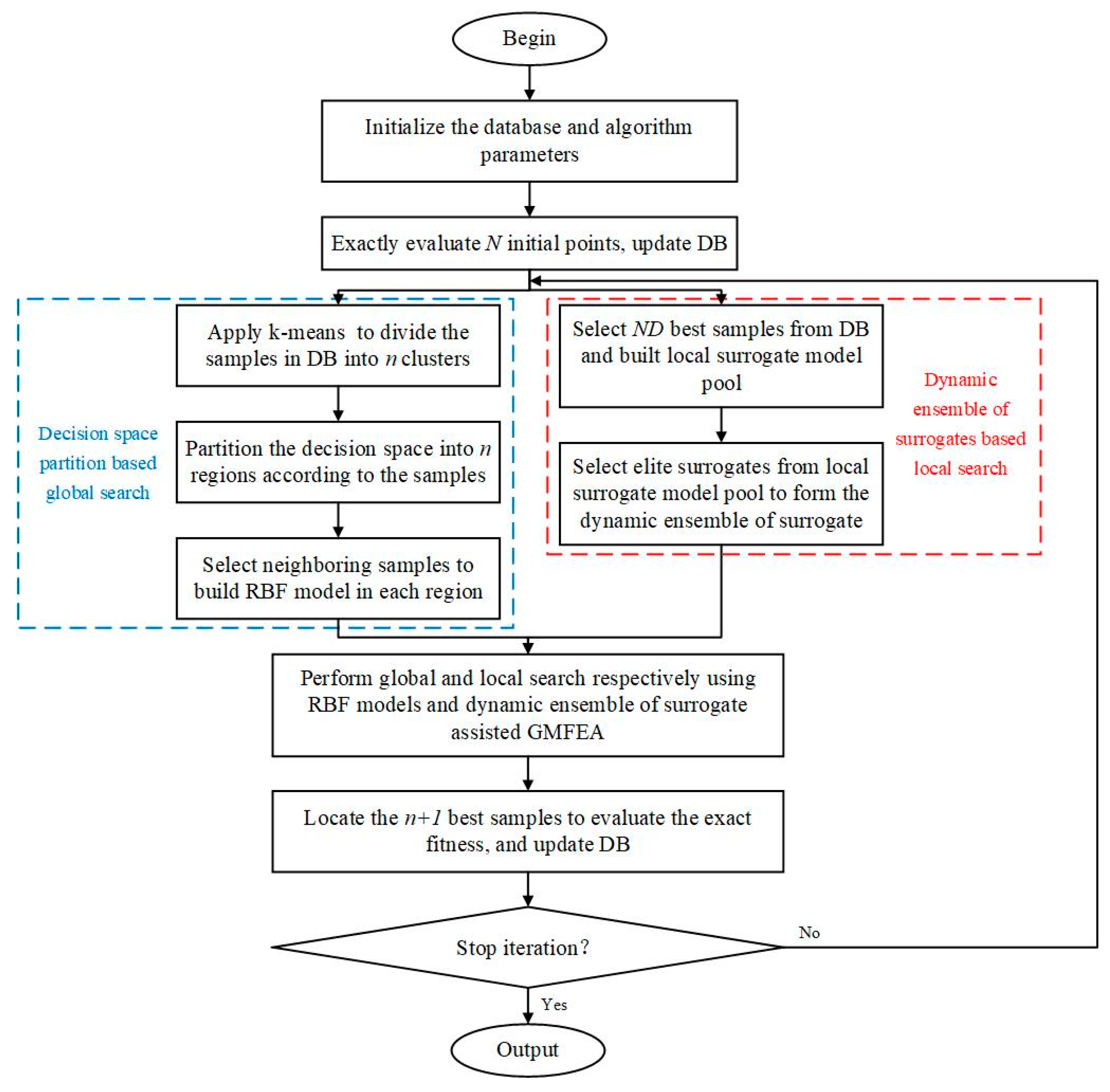
2.6.1. The General Framework of the MSAMT Method

The main algorithm design framework of the MSAMT is given in Figure 1. During the surrogate construction process, all of the samples in the database are first divided into $n$ clusters using k-means clustering to prevent SAEAs from entering local optima. Then, the entire space is divided into $n$ disjoint regions, and each of which is associated with a different cluster. Finally, a corresponding RBF model is constructed in each region to assist the optimizer in finding the promising point for the global search, and a dynamic ensemble of surrogates is constructed using the best part of the sample selected from the database to search for the promising point within the local region. The former is concerned with exploring the entire decision space, while the latter tends to exploit the subregion near the optimal individual. The promising points identified by the surrogate-assisted G-MFEA are accurately evaluated and added to the database (DB).

Figure 1. The flow chart of the proposed MSAMT.

Algorithm 1 provides the pseudocode of the MSAMT. Firstly, $N$ initial samples are sampled by Latin hypercube sampling (LHS). Each sample is evaluated by the real objective function and added to the DB. Secondly, all the exactly evaluated samples are clustered into $n$ groups utilizing k-means clustering, and the entire space is divided into $n$ disjoint areas based on the clusters. Then, the RBF model for each region is built. Thirdly, $ND$ samples having the optimal fitness values are chosen to construct a dynamic ensemble of surrogates proposed in Algorithm 2. Finally, $n+1$ surrogates are subsequently applied to help the G-MFEA in the population evolution of $k_{max}$ generations as shown in Algorithm 3. Algorithm 4 is applied to produce an initial evolutionary population. Individuals with superior fitness values predicted by the surrogates are exactly evaluated and archived in the DB. The global and local searches are conducted simultaneously, and each iteration locates $n$ promising points distributed in disjoint regions and one promising point in the region around the optimal individual. The entire process is repeated until the maximum number of FEs is exhausted.

Algorithm 1 Pseudocode of the MSAMT algorithm

Input: $D$, problem dimension; $N$, initial population size; $ND$, population size of dynamic ensemble of surrogates; $NP$, evolutionary population size; DB, database; $NFE$, the number of exact evaluations; ${NFE}_{max}$, the maximum number of exact evaluations; $f$, the real objective function; $n$, the number of clusters; rmp, matching probability; $k_{max}$, the maximum number for each running of multitasking optimization;

Output: the position of the best individual and its fitness value;

1: Generate $N$ initial samples by LHS;

2: Evaluate exactly $N$ initial samples by the real objective function and save them to the DB;

3: while $NFE<{NFE}_{max}$, do

4:   //Decision space partition based global search

5:   Randomly select $n$ samples from the DB as clustering centers;

6:   Calculate the distance between all samples in the DB and each clustering center and assign each sample to the clustering center nearest to it;

7:   Calculate the mean of each cluster as the new clustering center;

8:   Repeat rows 6 and 7 until the new center is unchanged from the original center and output $n$ central position;

9:   for $i=1$ to $n$, do

10:   Calculate the $r_i$ according to Equation (14);

11:  end for

12:  Determine in which region each of the samples in the database is located;

13:  for $i=1$ to $n$, do

14:   if the number of exactly evaluated samples distributed in the $i$th region is larger than $5\times D$, then

15:    Select all exactly evaluated samples in the $i$th region to construct the RBF surrogate model;

16:   else

17:    Select the $5\times D$ neighboring exactly evaluated samples to the $i$th region to construct the RBF surrogate model;

18:   end if

19:  end for

20:  //Dynamic ensemble of surrogates based local search

21:  Apply Algorithm 2 to construct a dynamic ensemble of surrogates;

22:  //Perform global and local searches using RBF models and the dynamic ensemble of the surrogate-assisted G-MFEA, respectively;

23:  Apply Algorithm 3 to generate an evolutionary population and let $k=0$;

24:  Apply Algorithm 4 to perform multi-tasking optimization;

25:  Locate the $n+1$ individuals having better predicted fitness;

26:  Evaluate the real fitness value of the $n+1$ best individuals and save them to the DB;

27:  $NFE=NFE+n+1$;

28: end while

Algorithm 2 Pseudocode for the dynamic ensemble of surrogates

Input: $ND$, population size of the dynamic ensemble of surrogates; DB, database;

Output: the dynamic ensemble of surrogates;

1: Apply $k$-fold cross validation (fivefold cross-validation is adopted in this paper) to $ND$ best samples in the DB and build a pool of different single surrogate models (denoted as ${\mathcal{M}}_{pool}$);

2: Compute the error metrics ($R^2$ and $NRMSE$) of these surrogates according to Equations (11) and (12);

3: Sort the $R^2$ and $NRMSE$ of these surrogates in ascending order and add the corresponding indices;

4: Add the $R^2$ and the $NRMSE$ indices for each surrogate together to obtain the final ranking indicator for all surrogates (denoted as ${\mathcal{M}}_{sort}$);

5: if $find \left({\mathcal{M}}_{sort}=2\right)$ is not empty, then

6:   Remove the other surrogates from ${\mathcal{M}}_{pool}$ and then use the single surrogate model with the ranking indicator of 2;

7: else $find \left({\mathcal{M}}_{sort}=3\right)$ is not empty

8:   if there are two surrogates with the ranking indicator of 3, then

9:   Remove the other surrogate from ${\mathcal{M}}_{pool}$ and formulate the two surrogates with the ranking indicator of 3 into an ensemble surrogate using the UES;

10:  end if

11: else

12:  Formulate the three surrogates into an ensemble surrogate using the UES;

13: end if

Algorithm 3 Pseudocode for multi-tasking optimization

Input: $N_p$, evolutionary population; $NP$, evolutionary population size; $k_{max}$, the maximum number for each running of multi-tasking optimization; $M_g$, the global surrogate model; $M_l$, the local surrogate model; $\theta$, the frequency to change the translation direction; $\phi$, the threshold value to start the decision variable translation strategy;

Output: the $n+1$ optimal solutions of surrogate models;

1: Apply Algorithm 4 to generate the evolutionary population and let $k=0$;

2: Predict the fitness of each individual in $N_p$ with the RBF surrogates and the ensemble surrogate;

3: Compute the skill factor ($\tau$) of each individual;

4: while $k<k_{max}$, do

5:   Randomize the individuals in $N_p$;

6:   for $i=1$ to $NP/2$, do

7:    Select two parent candidates $p_i$ and $p_{i+NP/2}$ from $N_p$;

8:    Generate a random number $r_1$, $r_2$, and $r_3$ between 0 and 1;

9:    if ${\tau }_i={\tau }_{i+NP/2}$ or $r_1<rmp$, then

10:    Parents $p_i$ and $p_{i+NP/2}$ crossover to give two offspring individuals $c_i$ and $c_{i+NP/2}$;

11:   else

12:    Mutate parent $p_i$ slightly to give an offspring $c_i$.

13:    Mutate parent $p_{i+NP/2}$ slightly to give an offspring $c_{i+NP/2}$;

14:   end if

15:   Assign skill factors by parent candidates to offspring through vertical cultural transmission;

16:   if $k>\phi$ and $mod (k, \theta )=0$, then

17:    Calculate the translated direction of each task;

18:   end if

19:   Update the position of each offspring according to the translated direction of its corresponding task;

20:  end for

21:  Predict the fitness of each offspring with the RBF surrogates and the ensemble surrogate and select better individuals as next parents;

22:  $k=k+1$;

23: end while

Algorithm 4 Pseudocode for generating the evolutionary population

Input: $NP$, evolutionary population size; DB, database; $num$, the number of samples in the DB;

Output: the evolutionary population $N_p$;

1: If $num<NP/4$, then

2:   Add all samples from the DB to $N_p$;

3:   Generate $NP-num$ individuals by LHS and add them to $N_p$;

4: else

5:   If $num<NP/2$, then

6:    Add the first sample from the DB to $N_p$;

7:    Randomly select $NP/4-1$ samples from other samples in the DB and add them to $N_p$;

8:   else

9:    Add the first sample from the DB to $N_p$;

10:   Randomly select $NP/4-1$ samples from 1 to $NP/2$ in the DB and add them to $N_p$;

11:  end if

12:  Generate $NP-NP/4$ individuals by LHS and add them to $N_p$;

13: end if

2.6.2. The Global and Local Models

The algorithm can be easily trapped into local optima because there are several local optima for various multimodal optimization problems. The proposed MSAMT adopts the method of decision space partition to help the optimization algorithm carry out global search. In this part of the work, we introduce the method suggested by Liu et al. [27] to partition the decision space. Firstly, all the samples in the database are divided into $n$ different clusters using the k-means clustering technique, i.e., $c_1,c_2,\cdots ,c_n$. Then, the decision space is divided into $n$ suitable disjoint regions according to each cluster. The radius of the $i$th region can be obtained as follows:

$$r_i={\displaystyle \frac{\underset{j=\left\{1,2,\cdots ,n\right\},j\ne i}{\mathit{max}}dis\left({cp}_i,{cp}_j\right)}{2{\sqrt{D}}^D\sqrt{\left(n-1\right)}}}$$

(14)

where ${cp}_i$ and ${cp}_j$ are the center positions of $c_i$ and $c_j$, respectively, $dis\left({cp}_i,{cp}_j\right)$ represents the Euclidean distance from ${cp}_i$ to ${cp}_j$, and $n$ and $D$ denote the number of clusters and input variables, respectively.

After the decision space is divided, the samples are selected from the DB to build RBF models (denoted as $M_g=\left\{M_g^1,M_g^2,\cdots ,M_g^n\right\}$) in each subregion separately. Given the $i$th region, if the number of accurately assessed samples in this region is greater than $5\times D$, all accurately assessed samples are chosen for modeling. Otherwise, the $5\times D$ neighboring accurately assessed samples to this region are selected for modeling.

As a dynamic ensemble of RBF, PRS, and SVR, the DES model has been used for high-dimensional optimization problems [28]. However, its accuracy and robustness need to be improved. On the one hand, the DES requires two parameters ${\left(R^2\right)}_{lb}$ and ${\left(R^2\right)}_{ub}$ to select appropriate component surrogates, which may make it not well suited for various optimization problems. For another, the DES makes the first selection of component surrogates by $R^2$ and then makes the second selection by $R^2$ or $NRMSE$ according to the number of remaining component surrogates in the first selection. Therefore, the DES may use only one error metric when selecting component surrogates, which may lead to deviations in the accuracy of the final ensemble surrogate.

To enhance the accuracy of the ensemble surrogate, a novel dynamic selection for the ensemble surrogate (DSES) is presented in this paper. Algorithm 2 provides the DSES technique in detail. The main distinctions between the DSES and the DES include the following two points. First, the DSES uses $R^2$ and $NRMSE$ error metrics simultaneously to select component surrogates, ensuring that the final components used to formulate the ensemble surrogate have better fitting performance. Second, the DSES selects component surrogates from two perspectives at the same time. Therefore, it does not need to limit surrogates by setting thresholds, avoiding the trouble of adjusting parameters. The final DSES (denoted as $M_l$) can be a single surrogate or an ensemble of two or three surrogates.

To demonstrate that the DSES has better performance than the DES, Figure 2 gives the $NRMSE$ values of both on the 20-dimensional F1 and F3 in the search process. From Figure 2, it was observed that the $NRMSE$ values of DSES and DES fluctuated greatly in the early period, but both gradually stabilized as the number of real function evaluations increased. Obviously, after stabilization, the DSES had smaller $NRMSE$ values than the DES. Therefore, one can consider that for different optimization problems, the DSES is more advantageous in building surrogate models with higher reliability than the DES.

Figure 2. The $NRMSE$ values of the DSES and the DES on functions F1 and F3 with 20 dimensions in the search process. (a) The $NRMSE$ values of the DSES and the DES on functions F1 with 20 dimensions in the search process; (b) The $NRMSE$ values of the DSES and the DES on functions F3 with 20 dimensions in the search process.

2.6.3. Multi-Tasking Optimization Based on Decision Space Partition and a Dynamic Ensemble of Surrogates

It has been demonstrated that multi-tasking optimization may effectively handle multiple optimization tasks simultaneously [30,31]. In this study, the generalized multi-factorial evolutionary algorithm (G-MFEA) [35] is utilized to identify the best solution. The G-MFEA is a generalization of the MFEA that adds two strategies, decision variable translation and decision variable shuffling, to promote knowledge transfer between optimization problems with different optimal solutions. The $n$ RBF models and one dynamic ensemble of surrogates are optimized simultaneously as $n+1$ tasks in the G-MFEA. The pseudocode for multi-tasking optimization is given in Algorithm 3.

In Algorithm 3, an evolutionary population $N_p$ with $NP$ individuals is generated at first, and the skill factors of them are computed by predicting fitness using $n$ RBF models and a dynamic ensemble of surrogates. The parent population generates an offspring population through an assortative mating strategy, subsequently utilizing vertical cultural transmission to designate skill factors to the offspring population. A decision variable transformation strategy is employed to map each offspring to a new location. The scalar fitness of the current populations is computed using surrogates, and then, individuals with better scalar fitness are chosen to become the next parent population. Algorithm 4 details the procedure of generating the initial evolutionary population. If the number of accurately assessed samples in the database is less than $NP/4$, all the samples in the database are added to the evolutionary population; if the number is greater than $NP/4$, but less than $NP/2$, $NP/4$ samples are randomly selected from the database to be added to the evolutionary population; otherwise, the $NP/2$ best samples are picked out from the database at first, and then, $NP/4$ samples are selected from them to be added to the evolutionary population. Finally, the LHS is used to generate the remaining evolutionary individuals. This initial evolutionary population is generated in such a way that both historical data and new data are included, which can lead to better algorithmic performance.

In addition, in order to avoid falling into the local optimality, this paper selects an individual with better fitness from the most promising and the average individual for exact evaluation and archiving in the database. The average individual is as follows:

$$\alpha ={\displaystyle \frac{NFE}{{NFE}_{max}}}$$

(15)

$$P={\displaystyle \frac{{\sum }_{i=1}^N{P}_i}{N}}\times \alpha \times \left|Gauss\left(\mathrm{0,1}\right)\right|$$

(16)

where $\alpha$ represents a parameter that rises with the number of exact evaluations, $N$ denotes the number of samples, and $Gauss\left(\mathrm{0,1}\right)$ denotes a random number that conforms to the Gaussian distribution.

3. Results and Discussion

A series of algorithm analyses will be taken to evaluate the performance of the MSAMT in this part. First, the test functions and parameters are provided, and the behavior of the MSAMT is studied in depth. Then, the MSAMT is contrasted with six recently proposed SAEAs, including HSAOA [28], DSP-SAEA [27], BiS-SAHA [25], FSAPSO [15], GL-SADE [21], and LSADE [22], on fourteen test functions and a practical engineering problem. Finally, the computational complexity of MSAMT is analyzed.

3.1. Test Problems

To study the effectiveness of the MSAMT, fourteen generally used test functions with different characteristics were adopted, and all of them considered five dimensions, namely 10D, 20D, 30D, 50D, and 100D. Table 2 provides the relevant details about these functions.

Table 2. Test functions used in the experiment study.

No.	Problem	Dimension	Optimum	Property
F1	Ellipsoid	10, 20, 30, 50, and 100	0	Unimodal
F2	Rosenbrock	10, 20, 30, 50, and 100	0	Multimodal with narrow valleys
F3	Ackley	10, 20, 30, 50, and 100	0	Multimodal
F4	Griewank	10, 20, 30, 50, and 100	0	Multimodal
F5	Rastrigin	10, 20, 30, 50, and 100	0	Multimodal
F6	Shifted Rotated High Conditioned Elliptic Function	10, 20, 30, 50, and 100	−450	Unimodal, shifted, rotated, and non-separable
F7	Shifted Rotated Ackley’s Function with Global Optimum on Bounds	10, 20, 30, 50, and 100	−140	Multimodal, shifted, rotated, and non-separable
F8	Shifted Rastrigin	10, 20, 30, 50, and 100	−330	Multimodal, shifted and separable
F9	Shifted Rotated Rastrigin	10, 20, 30, 50, and 100	−330	Very complicated multimodal
F10	Shifted Rotated Expanded Scaffer’s F6 (Shifted Rosenbrock’s Function) Function	10, 20, 30, 50, and 100	−300	Multimodal, shifted, and non-separable
F11	Rotated Hybrid Composition Function 1	10, 20, 30, 50, and 100	120	Very complicated multimodal
F12	Rotated Hybrid Composition Function 2	10, 20, 30, 50, and 100	10	Multimodal, rotated, and non-separable
F13	Rotated Hybrid Composition Function 2 with a Narrow Basin for the Global Optimum	10, 20, 30, 50, and 100	10	Very complicated multimodal
F14	Rotated Hybrid Composition Function 2 with the Global Optimum on the Bounds	10, 20, 30, 50, and 100	10	Multimodal, non-separable, and global optimum on the bound

3.2. Parameter Settings

In the MSAMT, for 10D, 20D, and 30D test functions, the initial population size $N$ was set to $5\times D$, the maximum number of exact function evaluations ${NFE}_{max}$ was set to $11\times D$, and the sample size $ND$ for training the ensemble surrogate was set to $2\times D$, which were the same as used in [28]. For 50D and 100D test functions, $N$ and $ND$ were both set to ${\displaystyle \frac{11}{10}}D$, and ${NFE}_{max}$ was set to 400. In the G-MFEA, the evolutionary population size $NP$ was set to 100 as used in [31], the iteration number for population evolution was set as $k_{max}=30$, and the mating probability was set as $rmp=0.4$. In addition, a vital parameter in the MSAMT is the number of clusters $n$, which was fixed at 2. To avoid randomness, each SAEAs was performed independently 20 times in MATLAB R2021b on the Intel Core i5-10400F with a 2.90 GHz processor to obtain the comparison results, and the MSAMT was compared to the other SAEAs using the Wilcoxon rank sum test (the significance level was set as $\alpha =0.05$) on fourteen test functions. The symbols, i.e., “+”, “-”, and “=“, show that the proposed MSAMT is superior, inferior, and competitive with the corresponding algorithms, respectively.

3.3. Behavior Study of the MSAMT

3.3.1. Effect of the Clusters Number

The clusters number $n$ is an important parameter in the MSAMT, and in order to study its impact on the MSAMT performance, we compared the outcomes of the MSAMT variants with varying $n$ values across the 10, 20, and 30 dimensions of the 14 test problems, as illustrated in Table A1.

Table A1 displays the results of the algorithm analysis, which demonstrated that different variants performed significantly differently when faced with the same test problems. For example, the MSAMT with $n=2$ outperformed the other variants on test problems such as F1, F4, and F5, the MSAMT with $n=5$ performed well on the F7 test function, and when $n=6$, the MSAMT outperformed on test functions such as F9 and F10. Comparing the results of all variants, it was found that the MSAMT with $n=2$ exhibited a superior performance on most of the test problems. Therefore, $n=2$ was used in this paper.

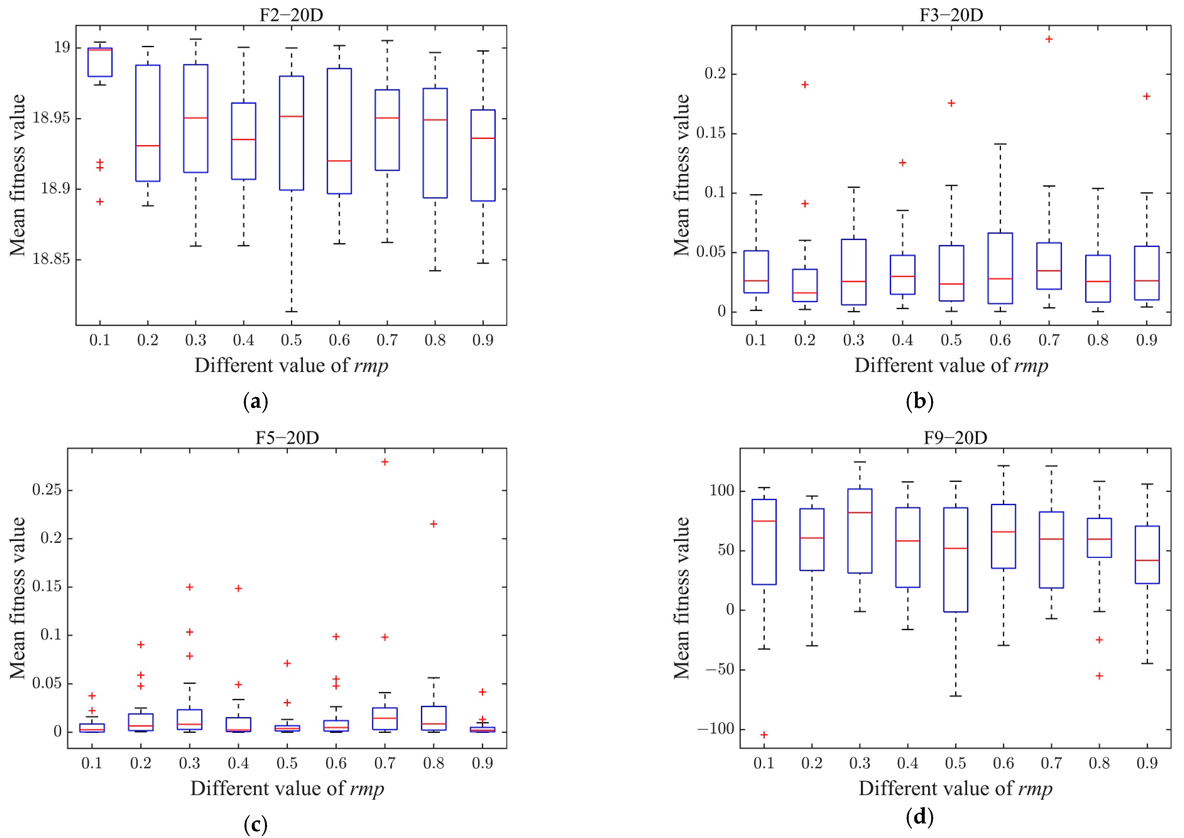
3.3.2. Effect of Matching Probability on Multi-Tasking Optimization

Exploration and exploitation capabilities determine how well the optimization algorithm performs. In the G-MFEA, the matching probability $rmp$ is used to achieve the balance between exploration and development. When $rmp$ is closer to 0, the probability of cross-task mating becomes smaller, thereby enhancing the exploitation ability. However, this may result in the algorithm converging on a local optimum. Conversely, when $rmp$ is closer to 1, the probability of cross-Zzztask mating increases, and it is able to search the decision space extensively, thus escaping from local optimality.

Figure 3 plots the mean fitness values of the MSAMT with different $rmp$ values on problems F2, F3, F5, and F9 with 20D. As Figure 3 shows, there was a considerable variation in the performance of MSAMT with different $rmp$ values. Without considering the red outliers, the MSAMT could obtain the best overall performance when the matching probability $rmp$ was equal to 0.4. Therefore, $rmp$ was set to 0.4 in this work.

Figure 3. Performances of the MSAMT with different $rmp$ values on 20D F2, F3, F5, and F9 (From (a) to (d) are the box plots of F1, F3, F5, and F9, respectively).

3.3.3. Effect of the Maximum Generation Number for Each Running of the G-MFEA

The maximum generation number $k_{max}$ for each running of the G-MFEA serves to balance the performance and optimization costs. A smaller $k_{max}$ may make it challenging for the algorithm to locate an improved solution, and a larger $k_{max}$ is beneficial for the discovery of the optimal solution but may result in an unaffordable running cost.

To achieve the optimal value of $k_{max}$ that achieves a balance between performance and optimization time, the same four test problems employed in the preceding section were utilized to assess the performance of the MSAMT variants with different $k_{max}$ values. Figure 4 displays the box plots of the average fitness values of the MSAMT variants with different $k_{max}$ values. It is evident from the Figure 4 that the medians, the maximum, and the interquartile range of the MSAMT were worse when the $k_{max}$ value was equal to 10 or 20. For different test problems, the performance of MSAMT with $k_{max}$ values greater than or equal to 30 displayed fluctuations, but the differences were not statistically significant. The maximum number of iterations for the G-MFEA was set to 50, taking into account both the optimization efficiency and the computing cost.

Figure 4. Performances of the MSAMT with different $k_{max}$ values on 20D F2, F3, F5, and F9 (From (a) to (d) are the box plots of F1, F3, F5, and F9, respectively).

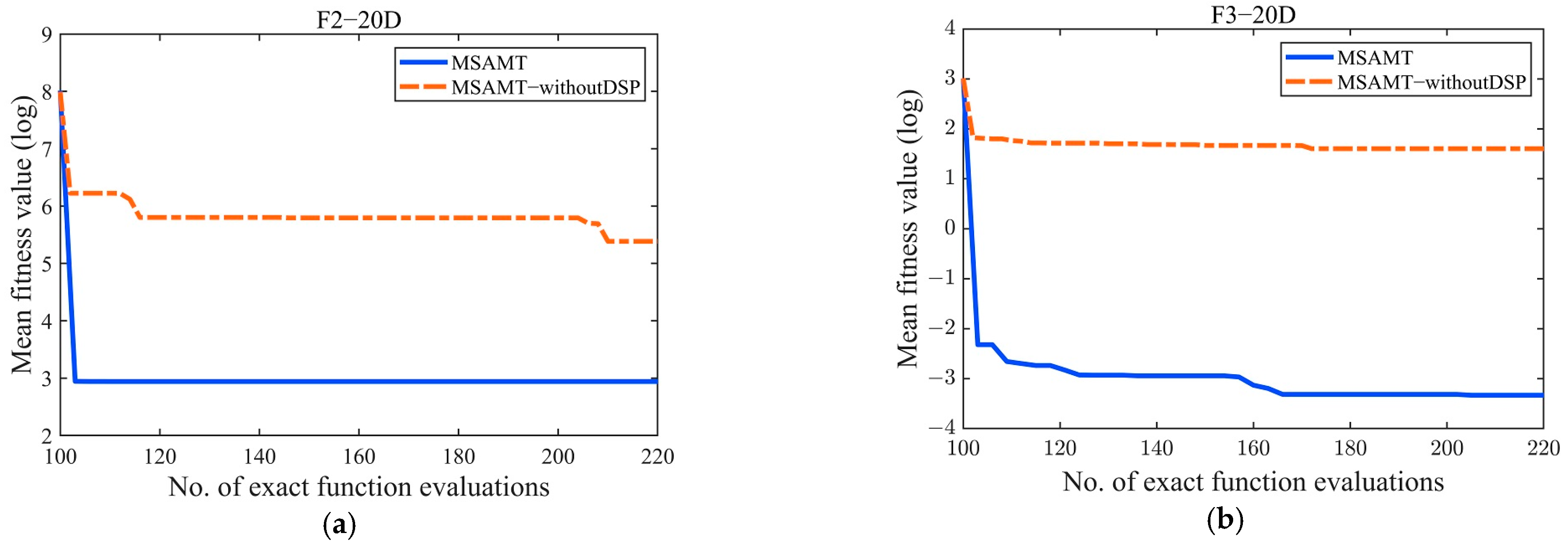
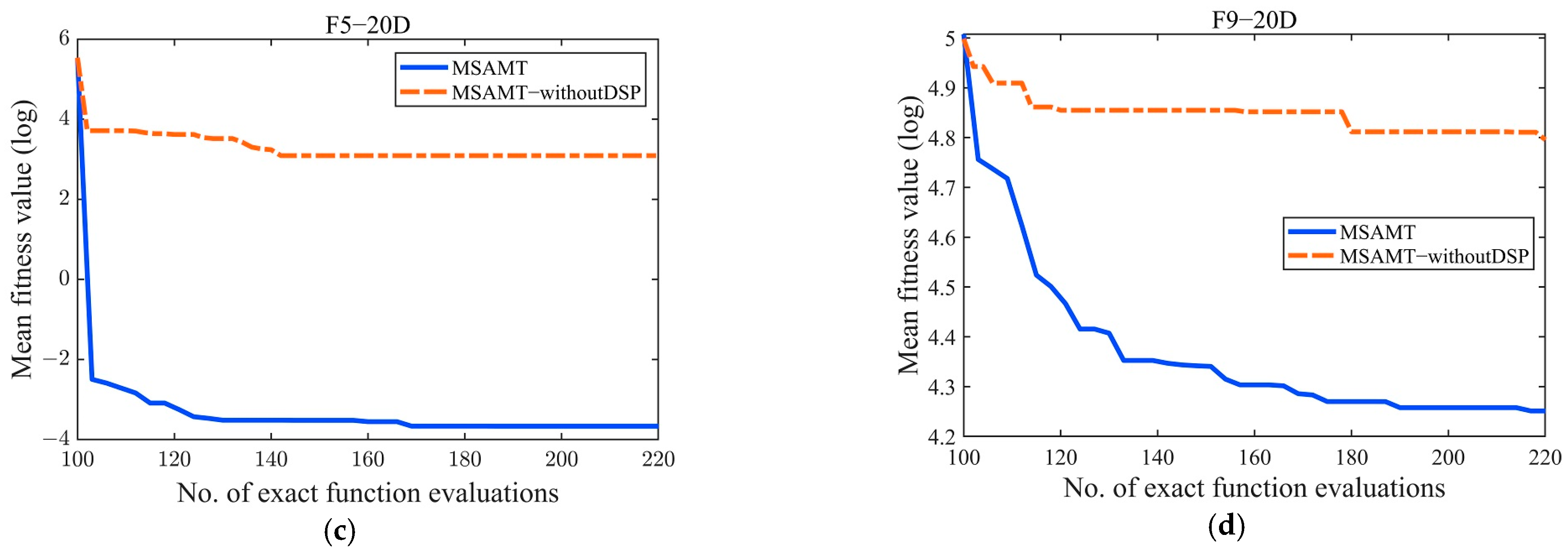
3.3.4. Effect of the Decision Space Partition

To evaluate the effectiveness of the decision space partition strategy, two variants, namely the proposed MSAMT and MSAMT-withoutDSP (only one RBF model is built to facilitate the global search conducted), were compared using the same four test functions as in Section 3.3.3. Figure 5 gives the convergence curves for the two variants. Figure 5 shows that the performance of the MSAMT was significantly better than MSAMT-withoutDSP without the decision space partition strategy. In particular, the MSAMT converged much faster than the MSAMT-withoutDSP in the early search stage.

Figure 5. Convergence curves of the MSAMT with/without decision space partition on 20D F2, F3, F5, and F9 (From (a) to (d) are the convergence curves of F1, F3, F5, and F9, respectively).

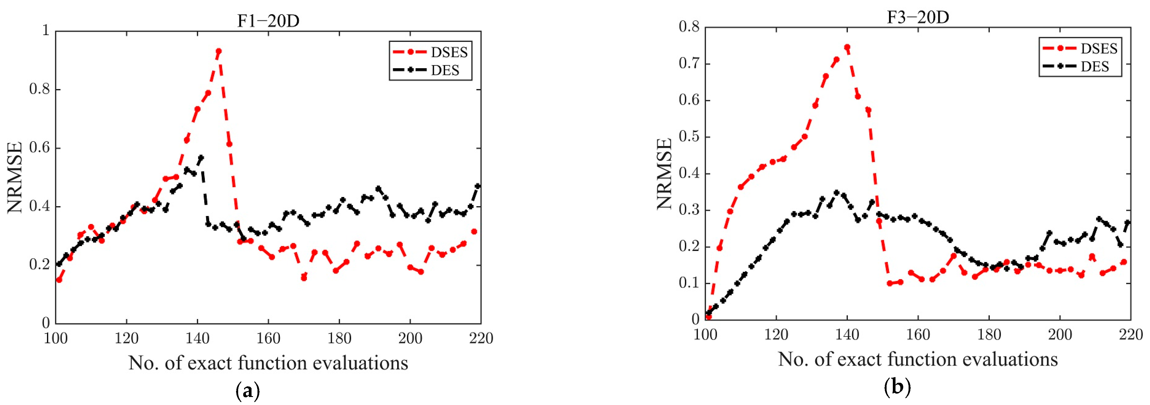
3.3.5. Effect of the DSES

To validate the impact of the DSES on the MSAMT, comparison studies of the proposed MSAMT and two various variants, i.e., the MSAMT-KRG which adopts the KRG model in local search and the MSAMT-fixed which carries out the original UES, were conducted on 20-dimensional test functions. Statistical results for the three variants are provided in Table A2. The MSAMT demonstrated a superior performance, achieving the best solution on 8 of the 14 test functions. The MSAMT-fixed beat the other two variants on four test functions, while the MSAMT-KRG exhibited the best results on two test functions. On all test functions, the MSAMT took less computational time than the other two variants. The results demonstrate the effectiveness of the DSES.

3.4. Comparison with Other Recently Proposed Algorithms

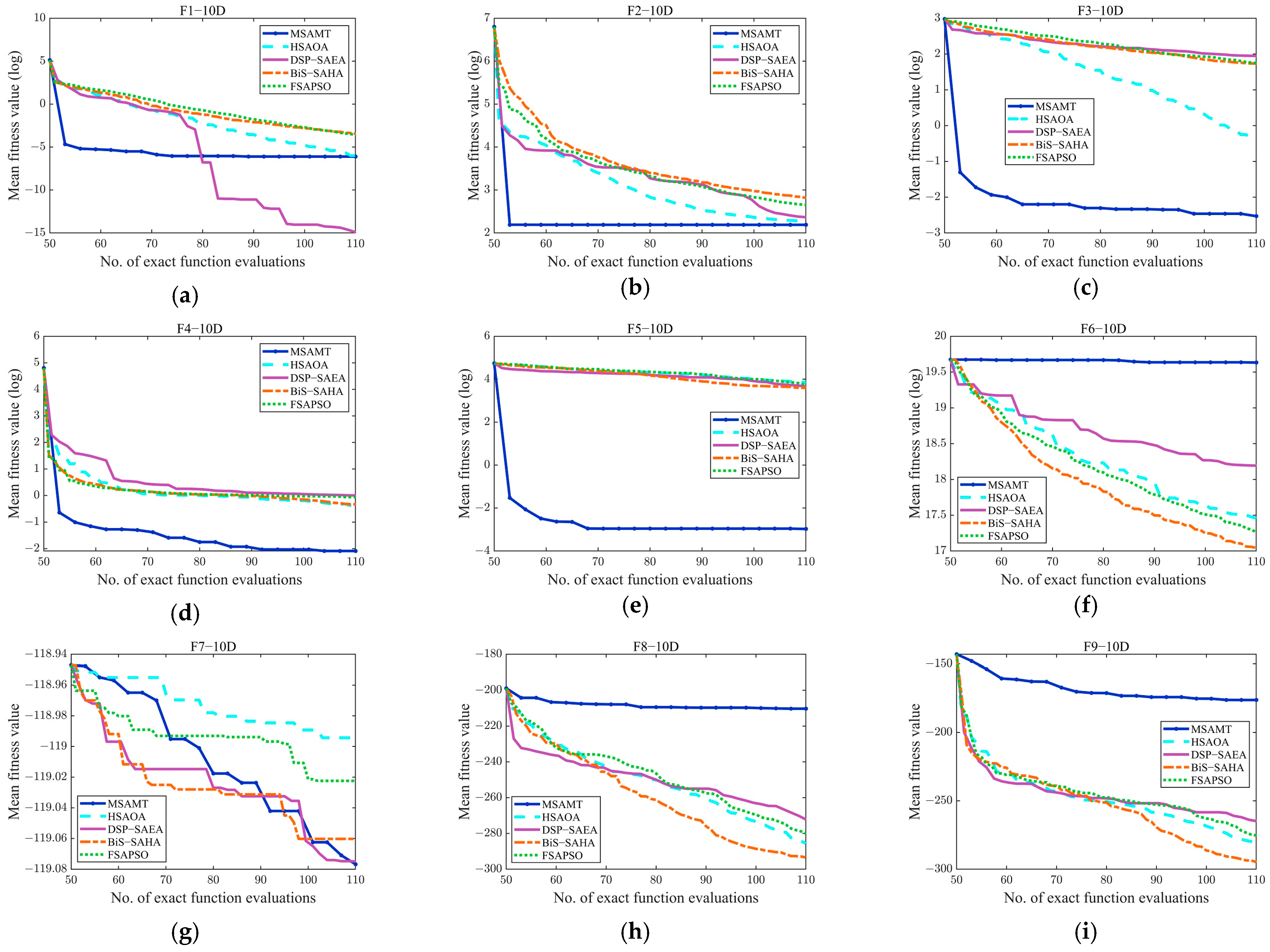
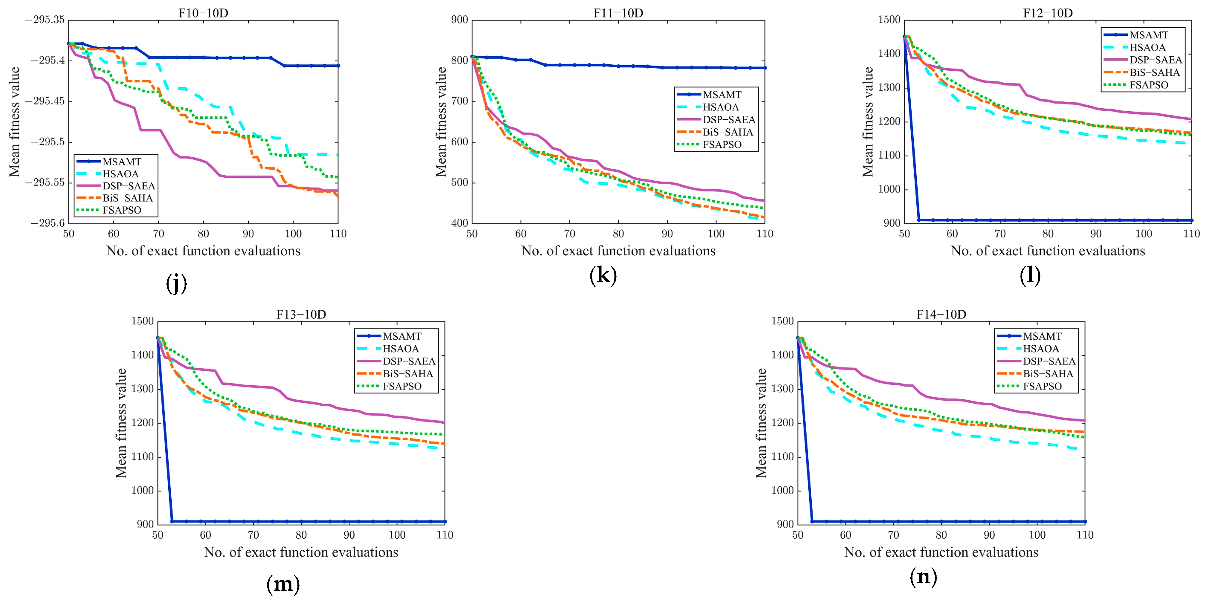
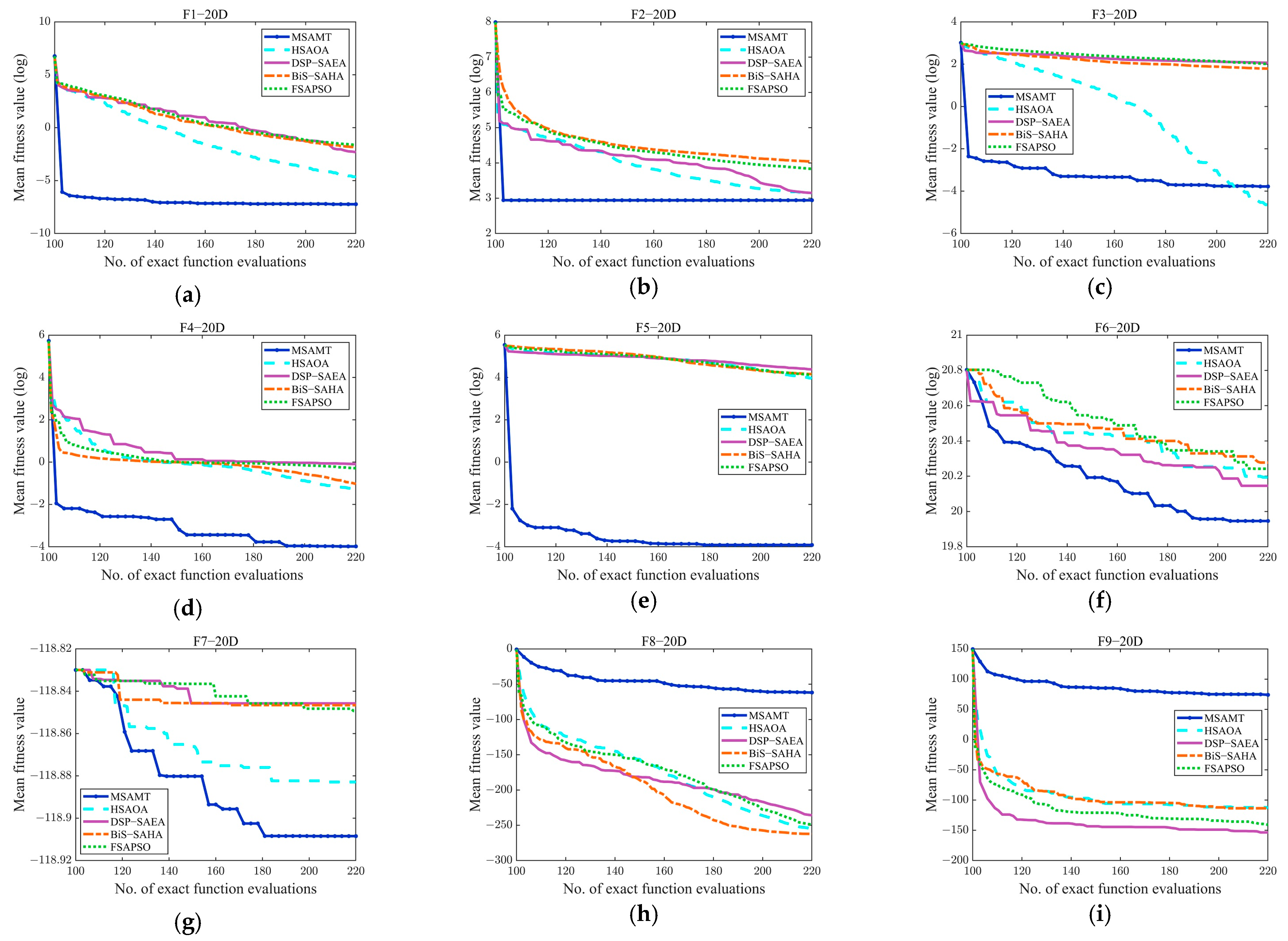
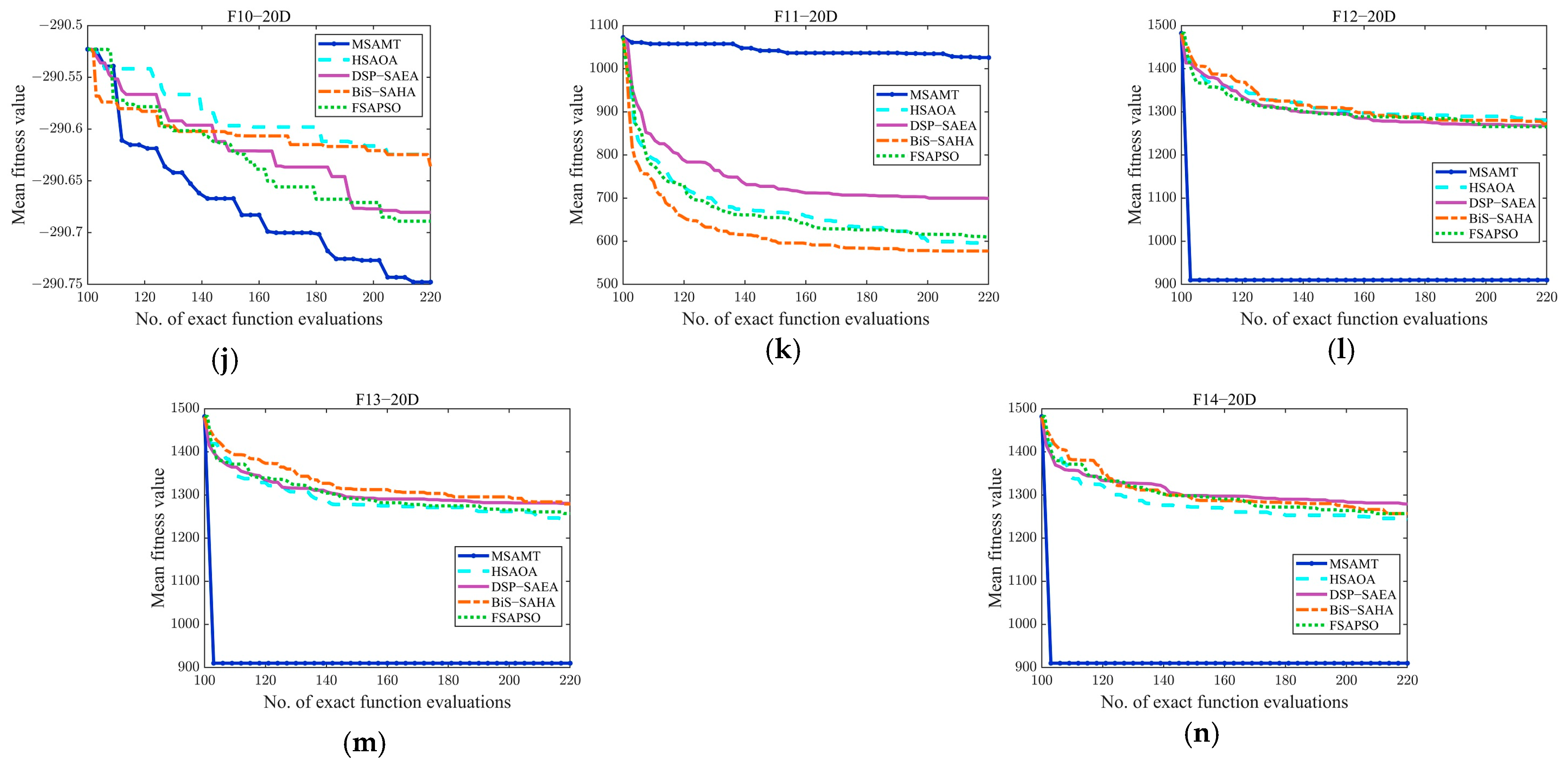
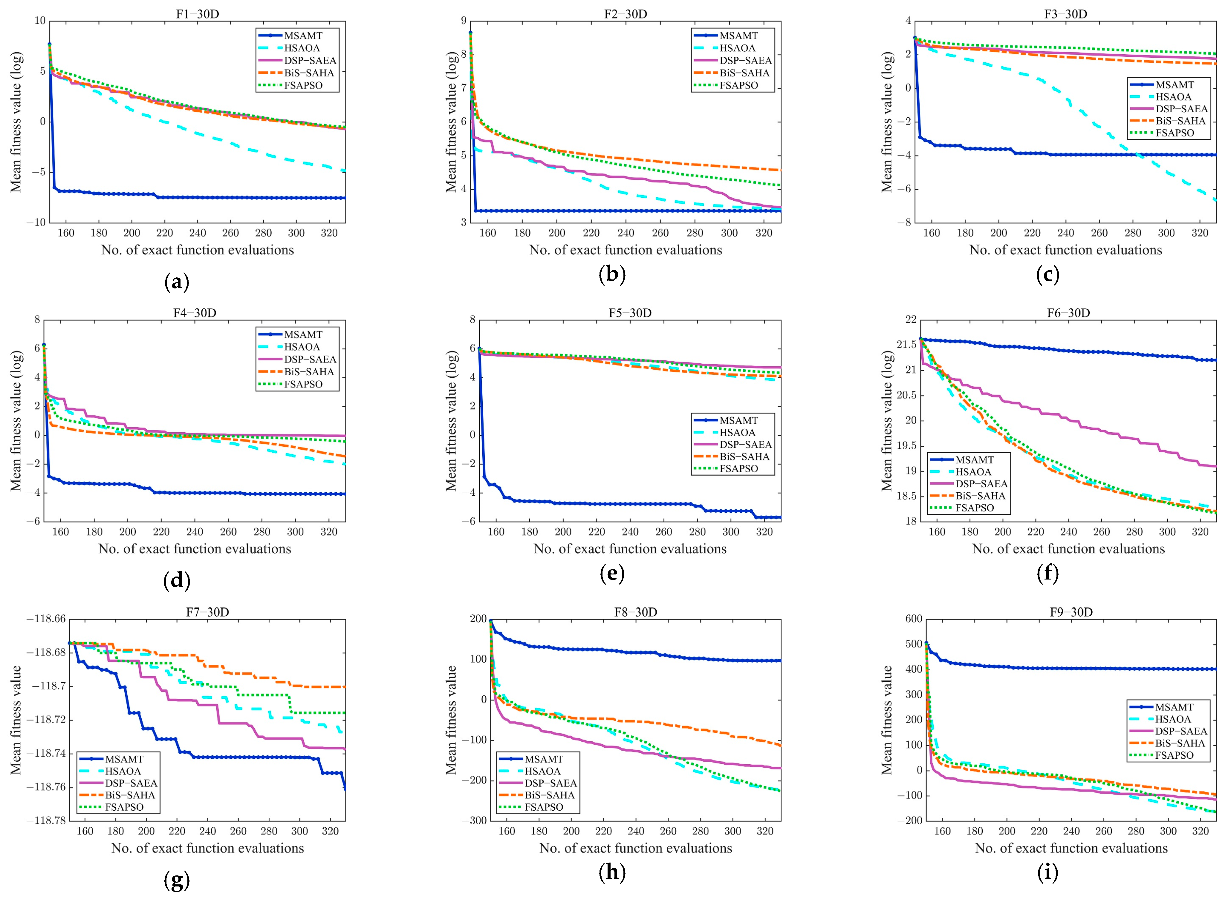
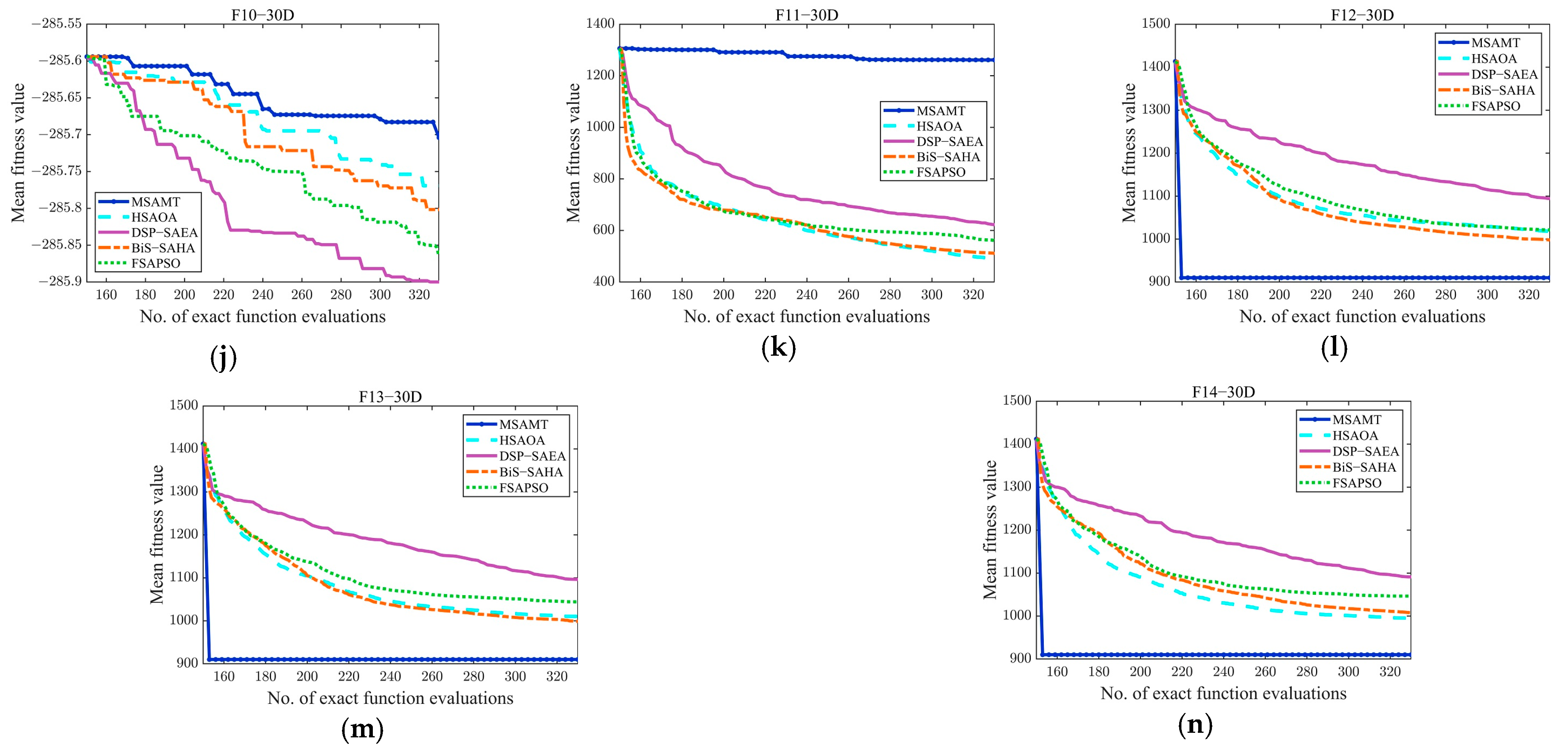
3.4.1. Experimental Results on 10D, 20D, and 30D Test Problems

Four recently proposed SAEAs were first selected as comparison algorithms, i.e., HSAOA, DSP-SAEA, BiS-SAHA, and FSAPSO, and they were compared with the proposed MSAMT on 10D, 20D, and 30D 14 test functions to evaluate the performance of the MSAMT. The HSAOA is a hierarchical surrogate-assisted optimization algorithm that alternately uses DE and TLBO. During the local search phase, the HSAOA selects the samples that are closest to the optimal solution or have the best fitness value to construct a novel dynamic ensemble of surrogates. The DSP-SAEA is a two-stage search algorithm that integrates the global search phase based on decision space partition strategy with the local search phase using an adaptive surrogate within the trust region. The BiS-SAHA performs the global and local search stages in turn using the SL-PSO assisted by a surrogate ensemble and RBF-assisted DE. The FSAPSO is a fast optimization technique using global RBF-assisted PSO that suggests a novel evaluation criterion to select particles for real function evaluation.

Table A3 demonstrates that the suggested MSAMT had a superior performance compared to the other SAEAs, with the best results on 26 functions and the second-best results on 3 functions. Compared with the HSAOA, the MSAMT had a better performance on 28 test problems. Both algorithms used a dynamic ensemble of surrogates developed from the same ensemble. However, the dynamic ensemble of surrogates proposed by the MSAMT had a better fitting performance, which is helpful for the algorithms to converge better. The MSAMT significantly outperformed the DSP-SAEA on 66.7% of the test functions. Despite the introduction of the decision space partition strategy from the DSP-SAEA into the global search, the MSAMT utilizes the G-MFEA to seek the optimal solution, thus facilitating information exchange between different decision space regions and preventing premature convergence to local optima. The MSAMT had a better performance than the BiS-SAHA on 31 out of 42 functions. Both use a surrogate ensemble, but the G-MFEA employed by the MSAMT enables the algorithm to converge better. The MSAMT had a better performance than FSAPSO on 73.8% of the test functions. The FSAPSO uses only the global RBF model, while the MSAMT simultaneously utilizes the RBF model and dynamic ensemble of surrogates, which makes the MSAMT perform better than the FSAPSO.

The convergence curves of the MSAMT and the four comparison algorithms on 10-, 20-, and 30-dimensional test functions are given in Figure A1, Figure A2 and Figure A3, respectively. According to the figures, the MSAMT outperformed the competing algorithms overall, with better convergence on most of the test functions. The preceding analysis indicates that MSAMT is competitive for low- and medium-dimensional problems.

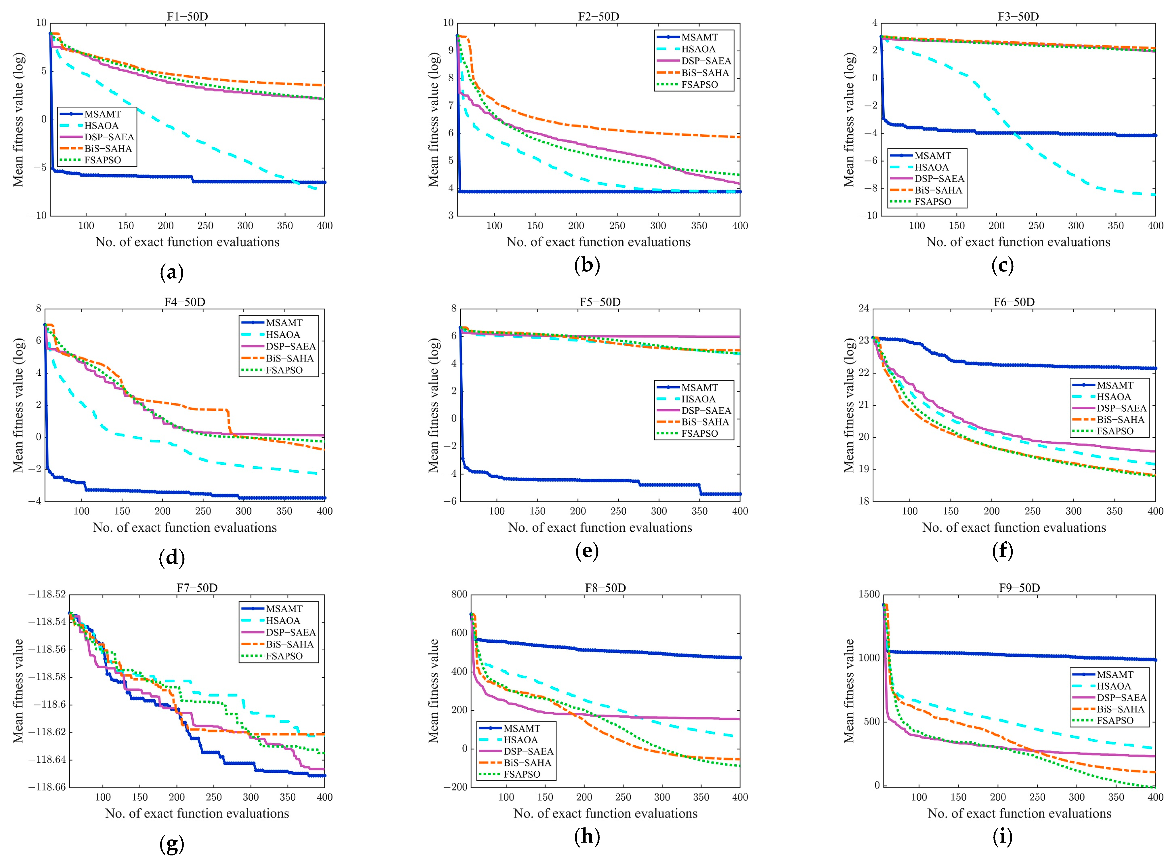
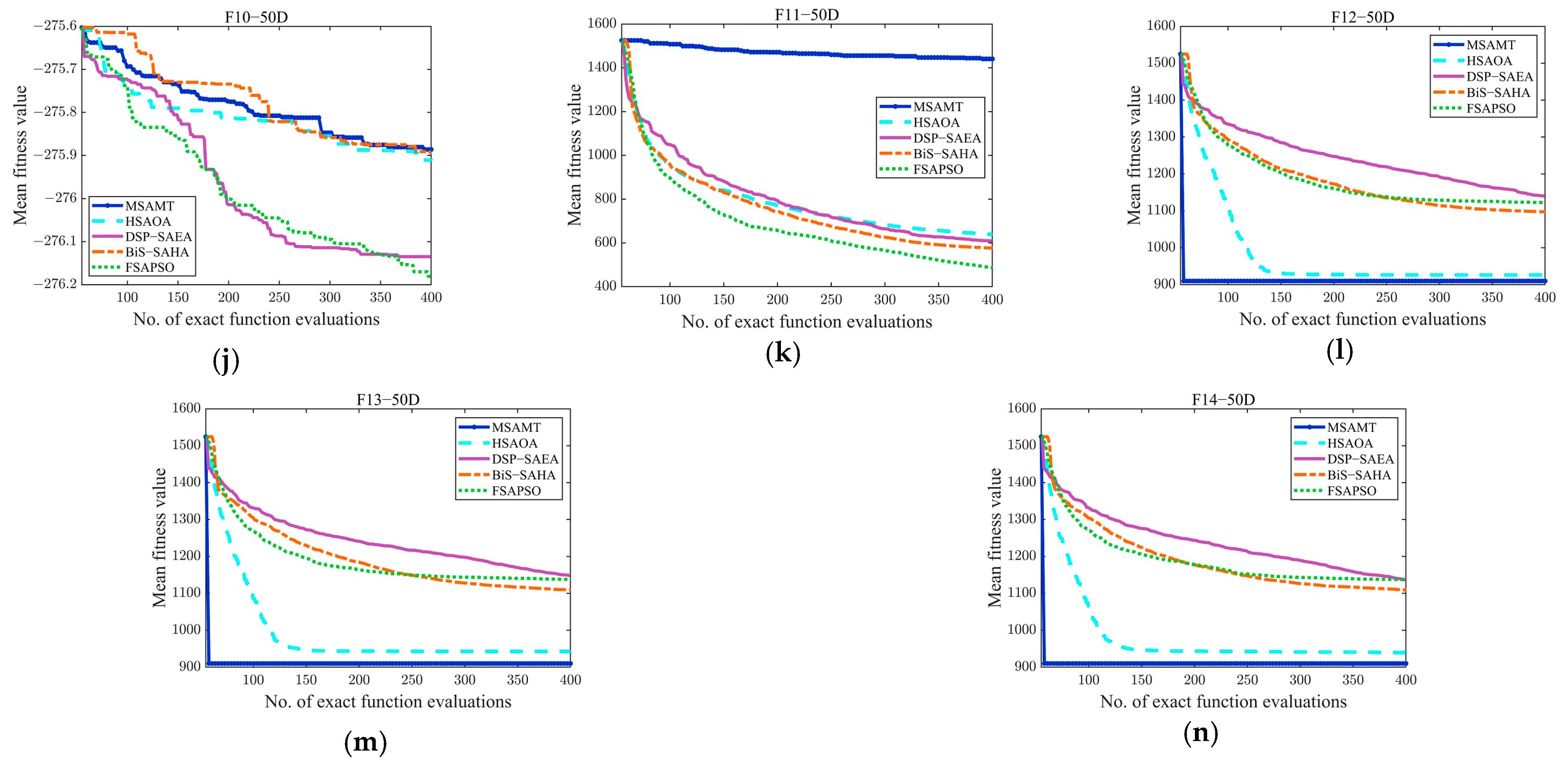
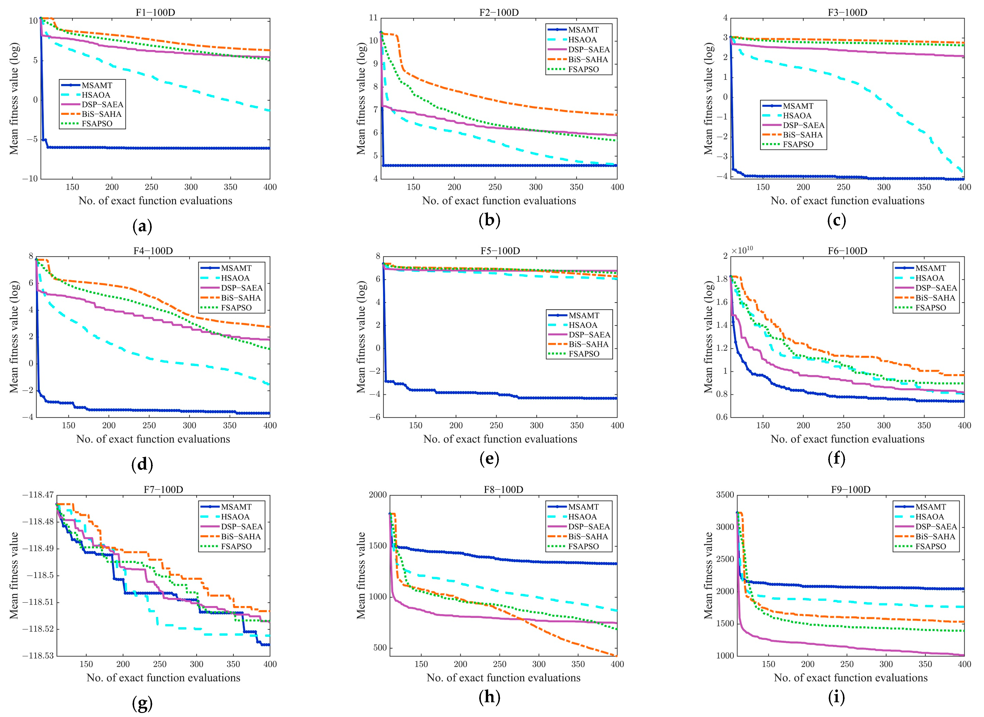
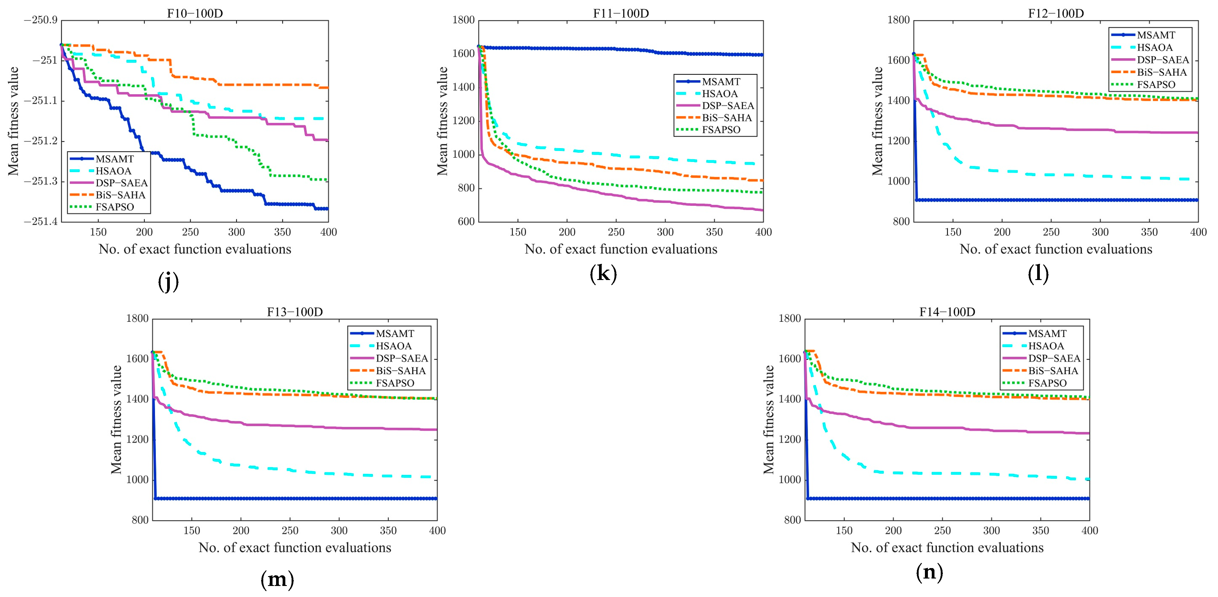
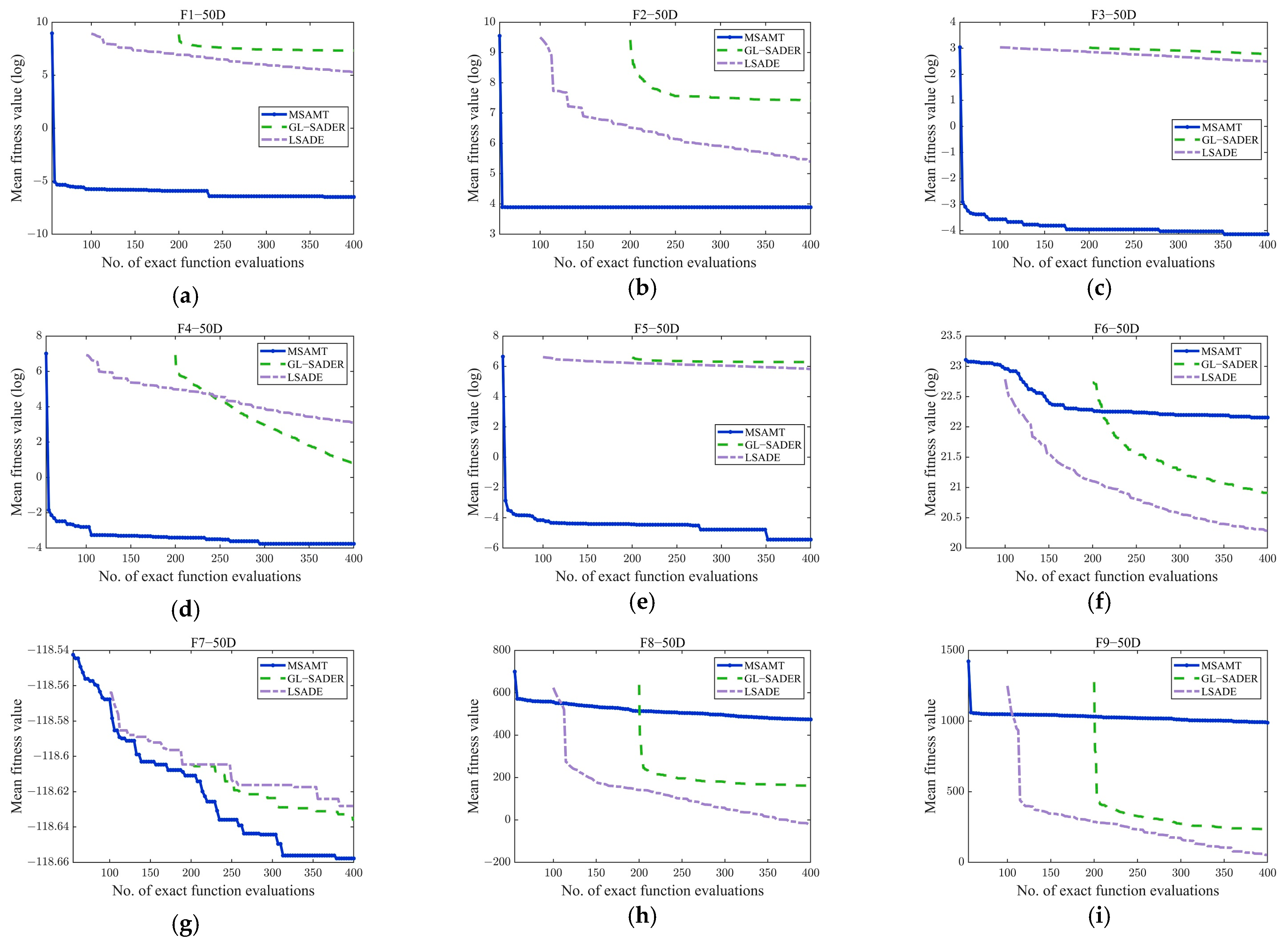
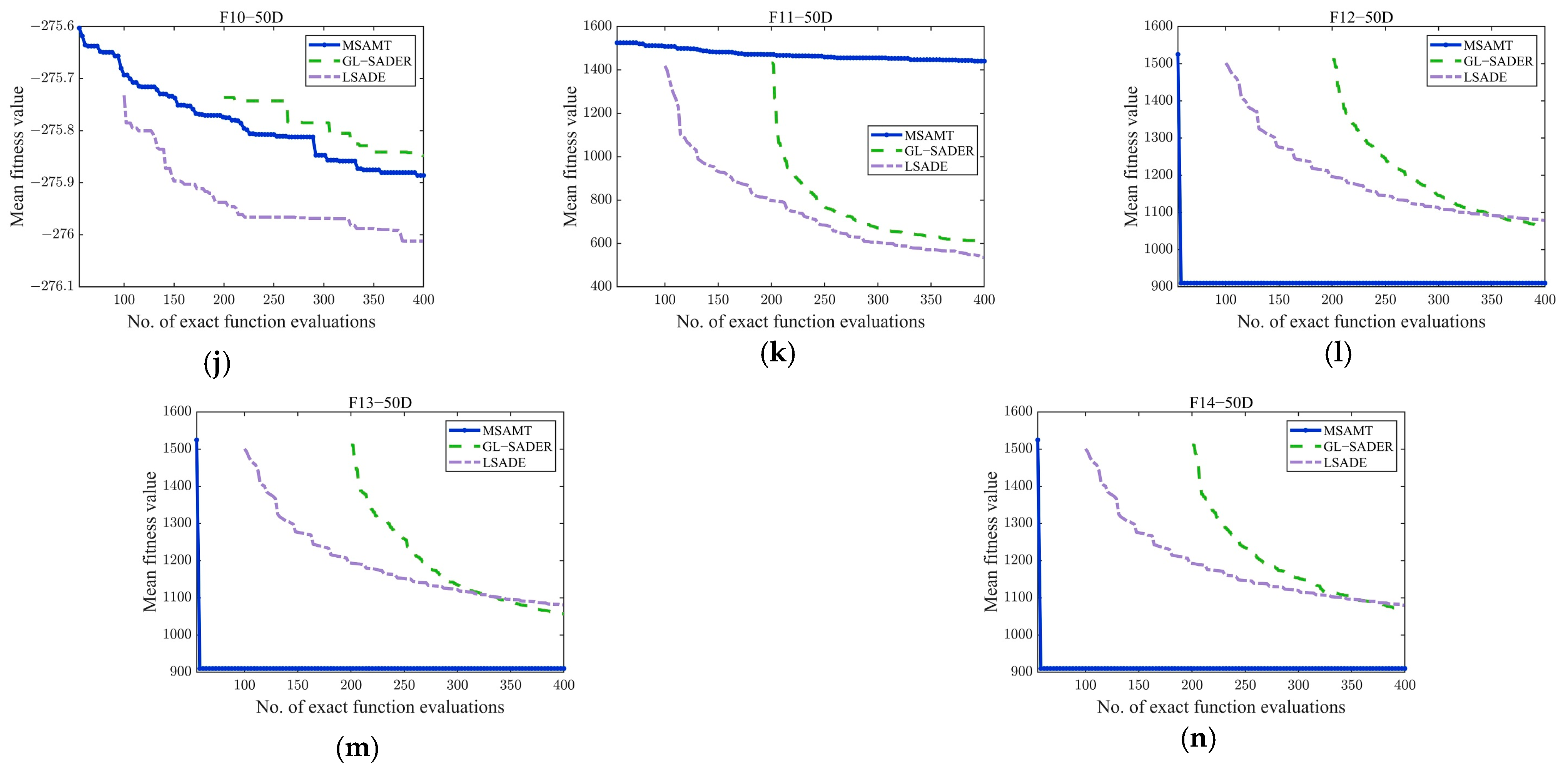
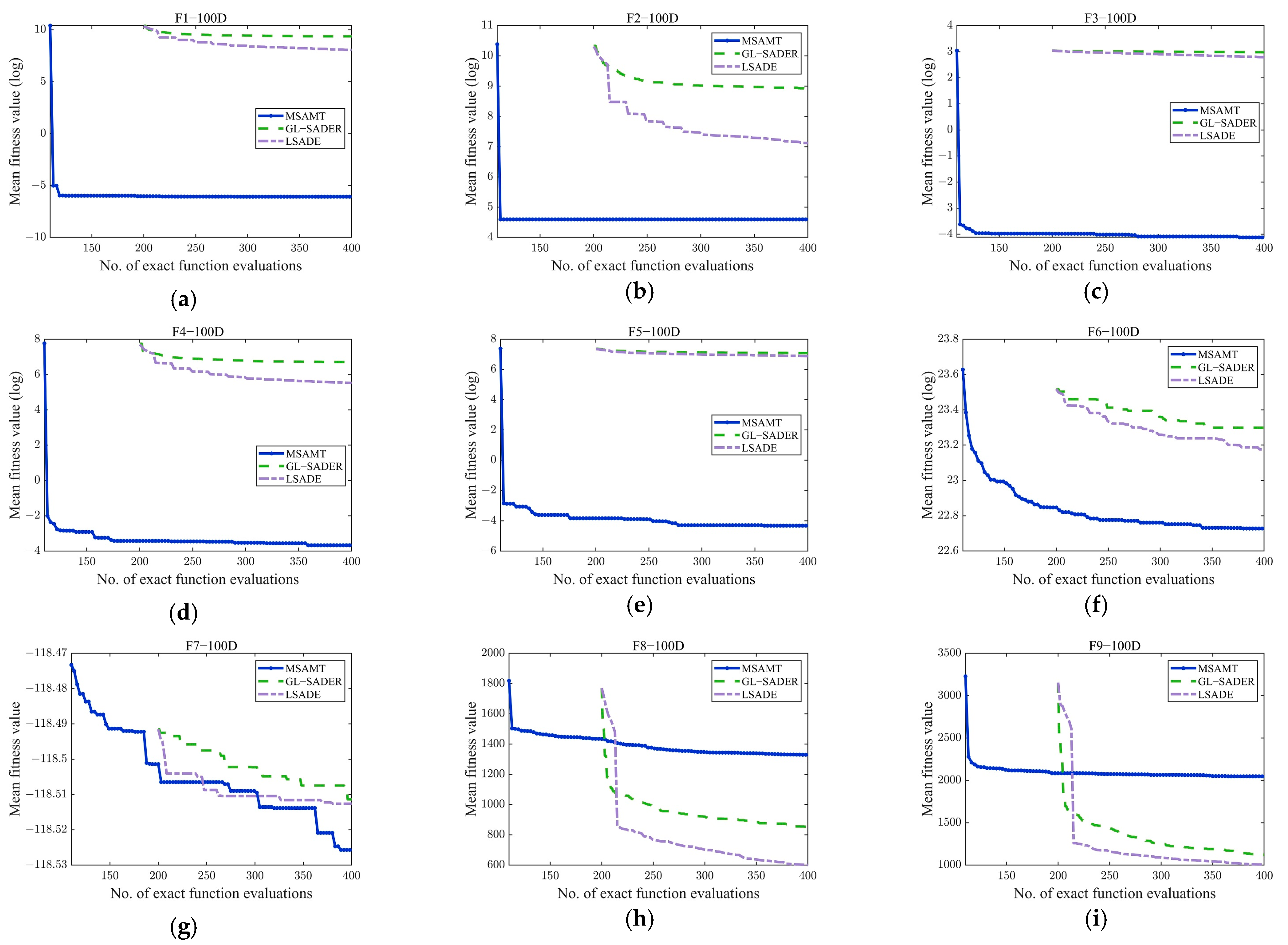
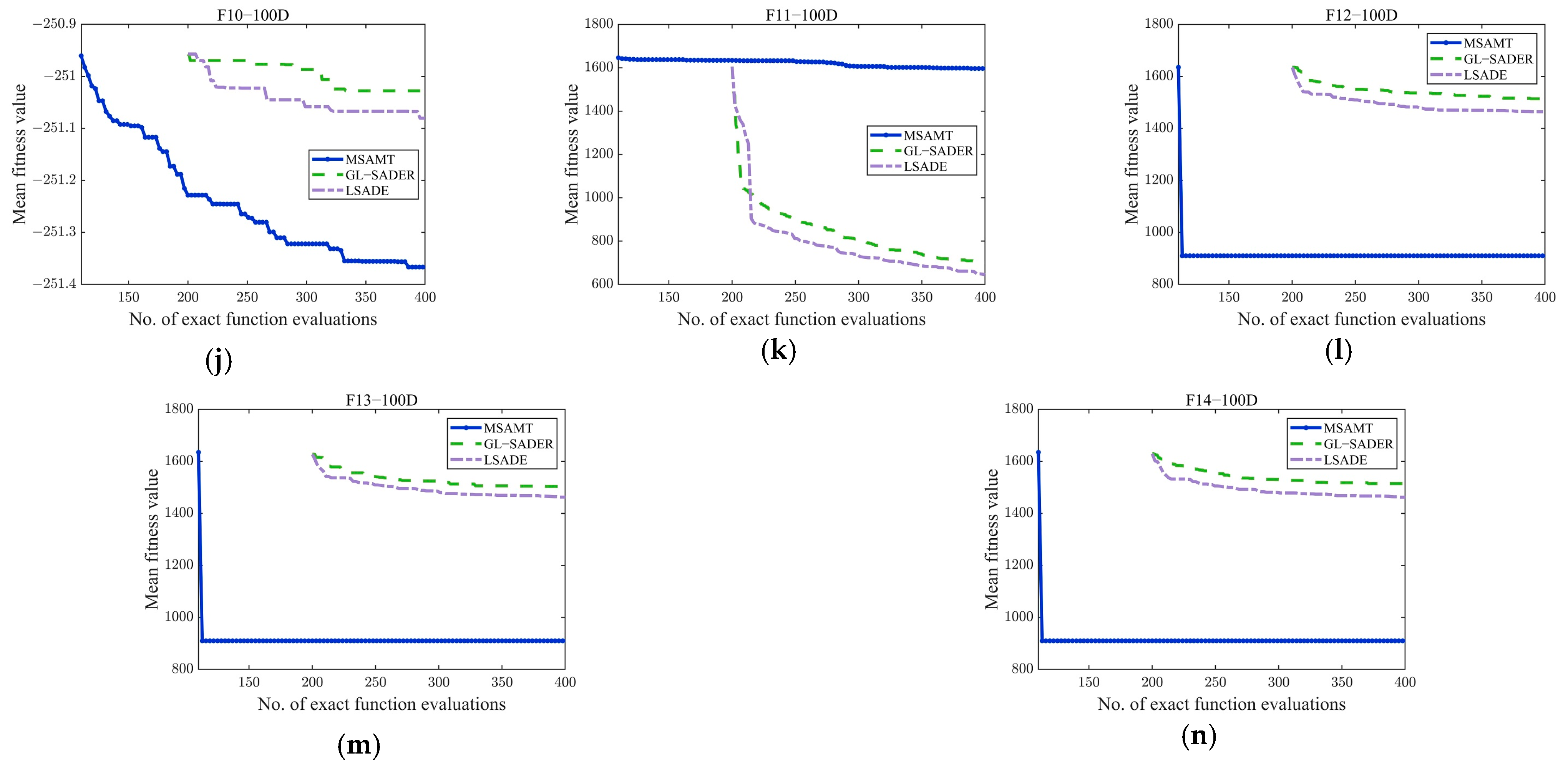
3.4.2. Experimental Results on 50D and 100D Test Problems

High-dimensional optimization problems are widely available in reality, and thus, this paper further validates the scalability of the MSAMT through 50D and 100D test problems. In addition to the four competing algorithms previously described, two additional algorithms are added in this section for comparison with the MSAMT, namely GL-SADE and LSADE. The GL-SADE alternately uses RBF and Kriging to assist DE to perform both global and local searches and then performs local searches again utilizing the rewarding mechanism if the local search yields a better result. The LSADE suggests a new surrogate model that is based on the Lipschitz and adopts DE as an optimization algorithm. Both the GL-SADE and LSADE were proposed for expensive optimization problems. Note that on 50D and 100D test problems, the initial population size $N$ for GL-SADE was set to 200, while for the LSADE it was set to 100 and 200.

Table A4 shows that the MSAMT achieved the optimal mean results on 60.7% of the test functions, thereby exhibiting a superior performance compared to the four competing SAEAs. For 18 of the 28 test functions, the MSAMT performed better than the HSAOA. Compared with the DSP-SAEA and the FSAPSO, the MSAMT achieved better results on 19 test functions. The MSAMT had a better performance than the FSAPSO on 71.4% of the functions. Table A5 presents the comparison results of the MSAMT with the GL-SADE and the LSADE on functions with 50 and 100 dimensions. The MSAMT obtained better results on 19 out of 28 functions. Compared with the GL-SADE, the MSAMT was more competitive on 20 test functions. In contrast to the LSADE, the MSAMT had better mean values on 19 test functions.

Convergence curves of the MSAMT, HSAOA, DSP-SAEA, BiS-SAHA, and FSAPSO for 50D and 100D test functions are given in Figure A4 and Figure A5, respectively. The figures demonstrate that the MSAMT had excellent convergence and could produce outcomes that are either better or comparable on most of the test functions. The HSAOA obtained the optimal results only on the F1-50 and F3-50 functions. The DSP-SAEA outperformed the other algorithms on the F9-100 and F11-100 functions, while the BiS-SAEA was most effective only for the F8-100 function. The FSAPSO obtained the best average value on five test problems, i.e., F6-50, F8-50, F9-50, F10-50, and F11-50. Figure A6 and Figure A7 show the convergence curves of MSAMT, GL-SADE, and LSADE on the 50- and 100-dimensional test problems, respectively. The MSAMT achieved the best mean values for all functions except F6-50, F8, F9, F10-50, and F11-50. The GL-SADE beat the other algorithms only on the F9-100 function. The LSADE won on 7 out of 28 functions. In summary, the MSAMT achieved the mean values on most of the test problems and was competitive in solving high-dimensional problems.

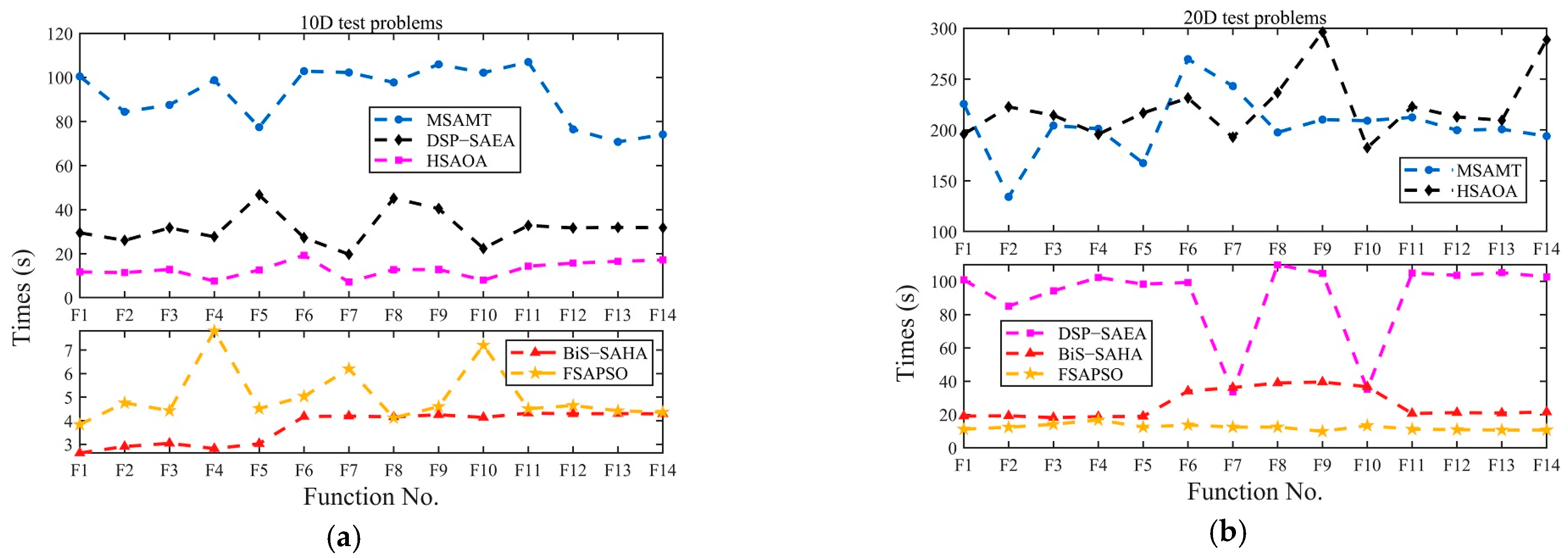
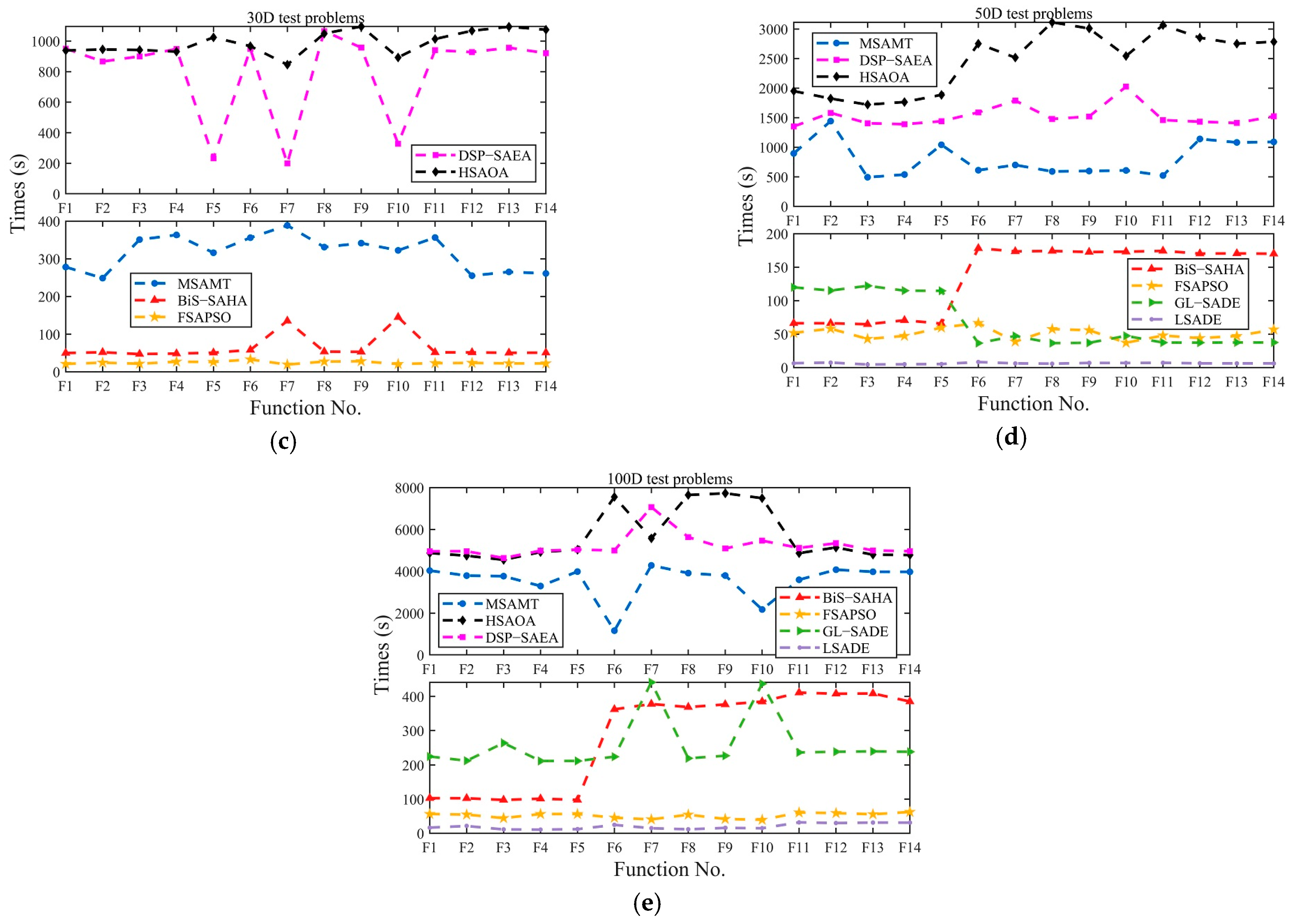
3.5. Computational Complexity Analysis of the MSAMT

Another essential part of measuring the performance of the algorithm is its computational complexity. The time complexity of the MSAMT is mainly determined by five main parts: the real function evaluation, the training of the dynamic ensemble of surrogates and the RBF models, the sorting of the samples in the database, the process of optimization using the G-MFEA, and other operations. The computational costs of other operations in the process are usually negligible, such as the generation and mutation of the population and the updating of the database.

Run times of the proposed MSAMT and six competing algorithms on 10-, 20-, 30-, 50-, and 100-dimensional test functions are given in Figure 6. Based on the statistics presented in Figure 6, it was evident that for the 10-dimensional functions, the BiS-SAHA consumed the least time, followed by the FSAPSO. For the 20- and 30-dimensional functions, the FSAPSO had the lowest time cost, followed by the BiS-SAHA. The LSADE took the least time on the 50- and 100-dimensional functions, while the HSAOA and the DSP-SAEA required significantly more time than the other algorithms. This is due to the fact that the FSAPSO, LSADE, and GL-SADE were constructed only with a single surrogate, whereas the BiS-SAHA, MSAMT, DSP-SAEA, and HSAOA all used a surrogate ensemble. The proposed MSAMT consumed the most time on the 10-dimensional test functions, but with the increasing of problem dimensions, its time cost was much lower than those of the HSAOA and the DSP-SAEA.

Figure 6. The average run times of the proposed algorithm and the competing algorithms on each test problem (From (a) to (e) are the average run times of 10D, 20D, 30D, 50D, and 100D test problems, respectively).

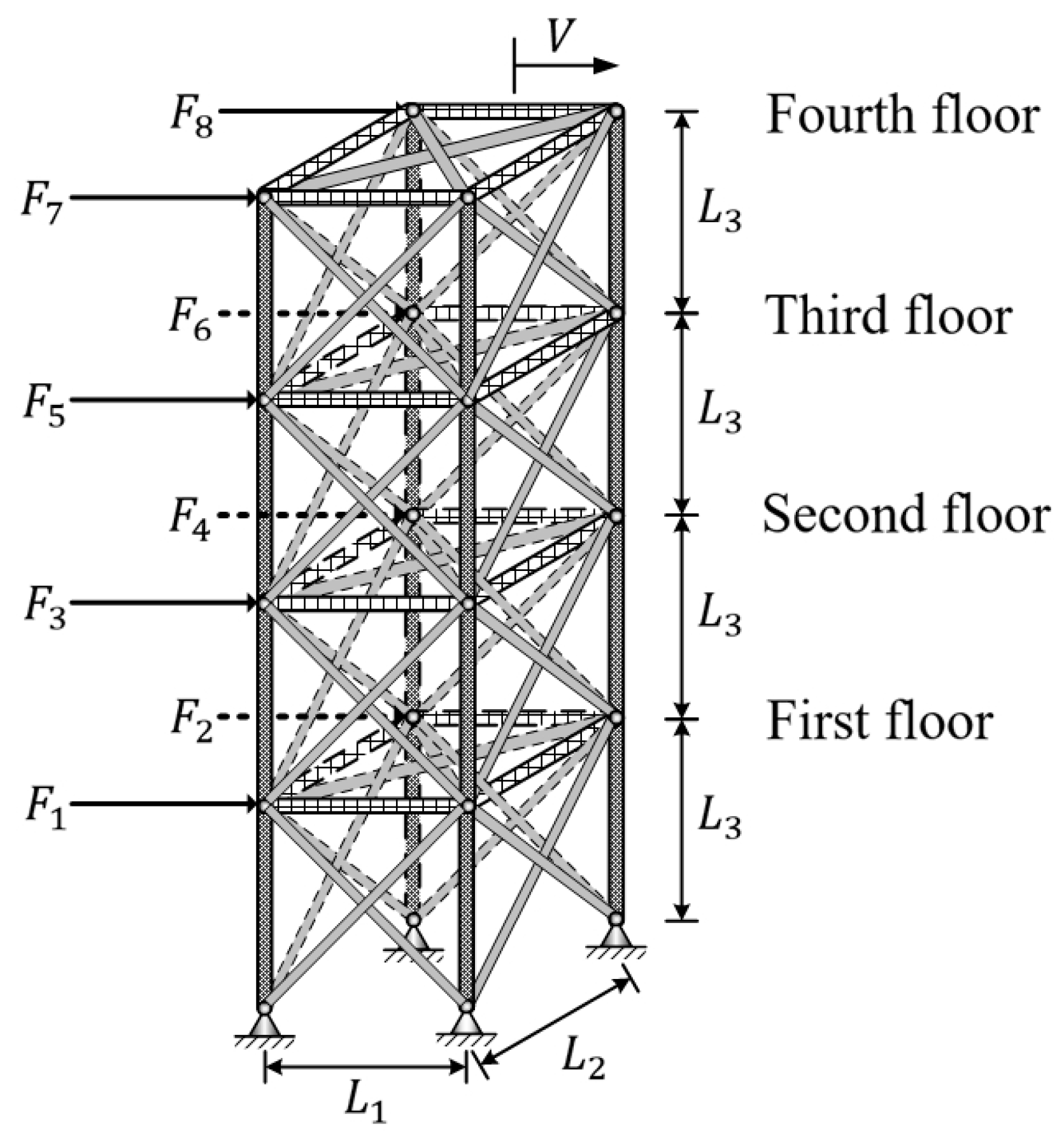
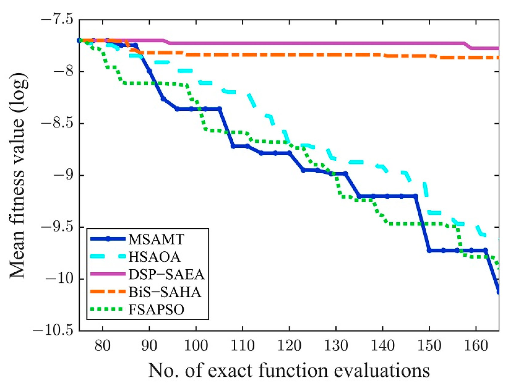
3.6. Case Study on a Spatial Truss Design Problem

Spatial truss design is representative in optimization design, which involves several design variables and is widely used to verify the prediction accuracy and robustness of different algorithms. In the following, the MSAMT proposed in this paper was applied to a spatial truss design problem and compared with existing algorithms. The design problem aimed to search for the best structural parameters under the maximum allowable horizontal displacement $V_{max}$, including the length of the horizontal, longitudinal, and vertical bars (denoted as $L_1$, $L_2$, and $L_3$), the Young’s modulus (denoted as $E_1$−$E_6$), and cross-sectional area (denoted as $A_1$−$A_6$) of the vertical, horizontal/longitudinal, and layer diagonal bars from the first to the fourth floor. Figure 7 shows the finite element model of the spatial truss structure comprising 72 bar elements under horizontal loads ($F_1~F_8$). The horizontal loads were fixed values set as $F_1=F_2=3.0\times \mathrm{N}$, $F_3=F_4=4.0\times \mathrm{N}$, and $F_5=F_6=5.0\times \mathrm{N}$. The initial values and ranges of the parameters to be optimized are shown in Table 3. The objective function to be optimized is given by the following:

$$\underset{\mathit{x}\in {\Omega }^d}{\mathit{min}}\left|V\left(\mathit{x}\right)-V_{max}\right| subject to: {\mathit{x}}_{lb}\le \mathit{x}\le {\mathit{x}}_{ub}$$

(17)

where $V$ represents the maximum horizontal displacement, $\mathit{x}$ is a vector containing the 15 parameters to be optimized, ${\mathit{x}}_{lb}$ and ${\mathit{x}}_{ub}$ are the upper and lower bounds of the parameters, respectively, and $d$ denotes the number of structural parameters ($d=15$).

Figure 7. Simulation diagram of the spatial truss structure.

Table 3. Initial values as well as upper and lower bounds of the parameters to be optimized.

Parameters	Initial Values	Upper Bounds	Lower Bounds
$L_1$/$L_2$/$L_3$	$1.0 \mathrm{m}$	$1.3 \mathrm{m}$	$0.7 \mathrm{m}$
$E_1$/$E_2$/$E_3$/$E_4$/$E_5$/$E_6$	$2.1\times \mathrm{P}\mathrm{a}$	$2.73\times \mathrm{P}\mathrm{a}$	$1.47\times \mathrm{P}\mathrm{a}$
$A_1$/$A_2$/$A_3$/$A_4$/$A_5$/$A_6$	$3.0\times {\mathrm{m}}^2$	$3.9\times {\mathrm{m}}^2$	$2.1\times {\mathrm{m}}^2$

The HSAOA, DSP-SAEA, BiS-SAHA, and FSAPSO were chosen as the competing algorithms. The relevant parameters remained constant with the configurations from the previous sections. The optimal structural parameters and statistical results of the MSAMT and the competing algorithms for the spatial truss structure design problem are given in Table A6 and Table 4, respectively. The data showed that MSAMT achieved the best results. The convergence history is given in Figure 8, and the MSAMT converged faster than the comparison algorithms. In conclusion, the above results show that MSAMT is highly competitive in solving real engineering optimal design problems.

Table 4. Statistical results obtained by the MSAMT, HSAOA, DSP-SAEA, BiS-SAHA, and FSAPSO on the spatial truss.

Methods	Statistical Results
	Best	Worst	Mean	Std
MSAMT	$1.01\times$	$1.42\times$	$4.00\times$	$4.05\times$
HSAOA	$2.29\times$	$2.57\times$	$6.72\times$	$6.44\times$
DSP-SAEA	$7.89\times$	$1.27\times$	$4.20\times$	$3.99\times$
BiS-SAHA	$7.89\times$	$1.61\times$	$3.85\times$	$4.74\times$
FSAPSO	$3.49\times$	$2.26\times$	$5.00\times$	$5.77\times$

Figure 8. Convergence curves of the MSAMT, HSAOA, DSP-SAEA, BiS-SAHA, and FSAPSO on the spatial truss.

4. Conclusions

This paper developed a multi-surrogate-assisted multi-tasking optimization algorithm (MSAMT) in the framework of the G-MFEA for the expensive optimization problems. The proposed MSAMT first divides the space into several disjoint regions using a decision space partition strategy and then builds an RBF model on each region. A new dynamic ensemble of surrogates is then suggested, constructed using the samples with the optimal fitness values. Several RBF models and a surrogate ensemble are then optimized simultaneously as tasks in multi-tasking optimization using the generalized multi-factorial evolutionary algorithm.

To evaluate the performance of the proposed approach, algorithm analyses of the MSAMT were first carried out on fourteen test functions, analyzing the parameters, the decision space partition strategy, the dynamic ensemble of surrogates, and the computational complexity. Finally, fourteen 10- to 100-dimensional test functions and a spatial truss design problem were used to compare the proposed approach with several recently proposed SAEAs. The results show that the proposed MSAMT exhibits a superior performance compared to comparison algorithms in most of the test functions and an engineering real-world problem.

The present study shows that the surrogate models can greatly affect the optimization results as they are utilized to select the samples that need to be evaluated exactly. Furthermore, as the modality of the optimization problem is increasing, both global and local searches may be unable to identify better individuals. Therefore, the proposed MSAMT enhances the population diversity through strategies such as the new dynamic ensemble of surrogates, the decision space partitioning, and the combination of local and global search under the G-MFEA framework to improve the performance of the algorithm.

In this work, the components used for constructing the ensemble surrogate are RBF, PRS, and SVR, and more components such as Kriging and the response surface model (RSM) could be further investigated to improve the ability of the MSAMT to handle various optimization problems. In addition, the control functions in the formula for calculating the weight coefficients (Equation (10)) can be adaptively selected according to different model combinations to further explore more reasonable weighting factors. Finally, it is possible to consider how the suggested MSAMT makes trade-offs between different objectives, thereby extending it to multi-objective optimization.

References

- Katoch, S.; Chauhan, S.S.; Kumar, V. A review on genetic algorithm: Past, present, and future. Multimedia Tools Appl. 2020, 80, 8091–8126. [Google Scholar] [CrossRef]
- Das, S.; Suganthan, P.N. Differential evolution: A survey of the state-of-the-art. IEEE Trans. Evol. Comput. 2011, 15, 4–31. [Google Scholar] [CrossRef]
- Yang, G.Y. A modified particle swarm optimizer algorithm. In Proceedings of the International Conference on Electronic Measurement and Instruments, Xi’an, China, 16–18 August 2007; pp. 2675–2679. [Google Scholar]
- Ong, Y.S.; Keane, A.J. Meta-Lamarckian learning in memetic algorithms. IEEE Trans. Evol. Comput. 2004, 8, 99–110. [Google Scholar] [CrossRef]
- Nelson, A.L.; Barlow, G.J.; Doitsidis, L. Fitness functions in evolutionary robotics: A survey and analysis. Robot. Auton. Syst. 2009, 57, 345–370. [Google Scholar] [CrossRef]
- Niyato, D.; Hossain, E. Dynamics of network selection in heterogeneous wireless networks: An evolutionary game approach. IEEE Trans. Veh. Technol. 2009, 58, 2008–2017. [Google Scholar] [CrossRef]
- Chai, R.; Savvaris, A.; Tsourdos, A.; Xia, Y.; Chai, S. Solving multiobjective constrained trajectory optimization problem by an extended evolutionary algorithm. IEEE Trans. Cybern. 2020, 50, 1630–1643. [Google Scholar] [CrossRef] [PubMed]
- Chai, R.; Tsourdos, A.; Savvaris, A.; Xia, Y.; Chai, S. Multiobjective optimal parking maneuver planning of autonomous wheeled vehicles. IEEE Trans. Ind. Electron. 2019, 67, 10809–10821. [Google Scholar] [CrossRef]
- Jin, Y.; Wang, H.; Chugh, T.; Guo, D.; Miettinen, K. Data-driven evolutionary optimization: An overview and case studies. IEEE Trans. Evol. Comput. 2019, 23, 442–458. [Google Scholar] [CrossRef]
- Shi, L.; Rasheed, K. A survey of fitness approximation methods applied in evolutionary algorithms. In Computational Intelligence in Expensive Optimization Problems; Springer: Berlin/Heidelberg, Germany, 2010; pp. 3–28. [Google Scholar]
- Branke, J.; Schmidt, C. Faster convergence by means of fitness estimation. Soft Comput. 2003, 9, 13–20. [Google Scholar] [CrossRef]
- Wang, X.; Wang, G.G.; Song, B.; Wang, P.; Wang, Y. A novel evolutionary sampling assisted optimization method for high-dimensional expensive problems. IEEE Trans. Evol. Comput. 2019, 23, 815–827. [Google Scholar] [CrossRef]
- Guo, D.; Jin, Y.; Ding, J.; Chai, T. Heterogeneous ensemble-based infill criterion for evolutionary multiobjective optimization of expensive problems. IEEE Trans. Cybern. 2019, 49, 1012–1025. [Google Scholar] [CrossRef]
- Yu, M.; Liang, J.; Wu, Z.; Yang, Z. A twofold infill criterion-driven heterogeneous ensemble surrogate-assisted evolutionary algorithm for computationally expensive problems. Knowl.-Based Syst. 2022, 236, 107747. [Google Scholar] [CrossRef]
- Li, F.; Shen, W.; Cai, X.; Gao, L. A fast surrogate-assisted particle swarm optimization algorithm for computationally expensive problems. Appl. Soft Comput. 2020, 92, 106303. [Google Scholar] [CrossRef]
- Li, F.; Cai, X.; Gao, L.; Shen, W. A surrogate-assisted multiswarm optimization algorithm for high-dimensional computationally expensive problems. IEEE Trans. Cybern. 2021, 51, 1390–1402. [Google Scholar] [CrossRef]
- Nourian, N.; El-Badry, M.; Jamshidi, M. Design optimization of truss structures using a graph neural network-based surrogate model. Algorithms 2023, 16, 380. [Google Scholar] [CrossRef]
- Cai, X.; Gao, L.; Li, X. Efficient generalized surrogate-assisted evolutionary algorithm for high-dimensional expensive problems. IEEE Trans. Evol. Comput. 2020, 24, 365–379. [Google Scholar] [CrossRef]
- Pan, J.S.; Liu, N.; Chu, S.C.; Lai, T. An efficient surrogate-assisted hybrid optimization algorithm for expensive optimization problems. Inf. Sci. 2021, 561, 304–325. [Google Scholar] [CrossRef]
- Sun, C.; Jin, Y.; Zeng, J.; Yu, Y. A two-layer surrogate-assisted particle swarm optimization algorithm. Soft Comput. 2014, 19, 1461–1475. [Google Scholar] [CrossRef]
- Wang, W.; Liu, H.L.; Tan, K.C. A surrogate-assisted differential evolution algorithm for high-dimensional expensive optimization problems. IEEE Trans. Cybern. 2023, 53, 2685–2697. [Google Scholar] [CrossRef]
- Kůdela, J.; Matoušek, R. Combining Lipschitz and RBF surrogate models for high-dimensional computationally expensive problems. Inf. Sci. 2023, 619, 457–477. [Google Scholar] [CrossRef]
- Rumpfkeil, M.P.; Bryson, D.; Beran, P. Multi-fidelity sparse polynomial chaos and kriging surrogate models applied to analytical benchmark problems. Algorithms 2022, 15, 101. [Google Scholar] [CrossRef]
- Liu, N.; Pan, J.S.; Chu, S.C.; Lai, T. A surrogate-assisted bi-swarm evolutionary algorithm for expensive optimization. Appl. Intell. 2022, 53, 12448–12471. [Google Scholar] [CrossRef]
- Ren, Z.; Sun, C.; Tan, Y.; Zhang, G.; Qin, S. A bi-stage surrogate-assisted hybrid algorithm for expensive optimization problems. Complex Intell. Syst. 2021, 7, 1391–1405. [Google Scholar] [CrossRef]
- Li, X.; Li, S. An adaptive surrogate-assisted particle swarm optimization for expensive problems. Soft Comput. 2021, 25, 15051–15065. [Google Scholar] [CrossRef]
- Liu, Y.; Liu, J.; Tan, S. Decision space partition based surrogate-assisted evolutionary algorithm for expensive optimization. Expert Syst. Appl. 2023, 214, 119075. [Google Scholar] [CrossRef]
- Zhang, J.; Li, M.; Yue, X.; Shi, M. A hierarchical surrogate assisted optimization algorithm using teaching-learning-based optimization and differential evolution for high-dimensional expensive problems. Appl. Soft Comput. 2024, 152, 111212. [Google Scholar] [CrossRef]
- Wu, G.; Mallipeddi, R.; Suganthan, P.N. Ensemble strategies for population-based optimization algorithms–A survey. Swarm Evol. Comput. 2019, 44, 695–711. [Google Scholar] [CrossRef]
- Liao, P.; Sun, C.; Zhang, G.; Jin, Y. Multi-surrogate multi-tasking optimization of expensive problems. Knowl.-Based Syst. 2020, 205, 106262. [Google Scholar] [CrossRef]
- Yang, S.; Qi, Y.; Yang, R.; Ma, X.; Zhang, H. A surrogate assisted evolutionary multitasking optimization algorithm. Appl. Soft Comput. 2023, 132, 109775. [Google Scholar] [CrossRef]
- Akopov, A.S.; Hevencev, M.A. A multi-agent genetic algorithm for multi-objective optimization. In Proceedings of the IEEE International Conference on Systems, Man, and Cybernetics, Manchester, UK, 13–16 October 2013. [Google Scholar]
- Zhong, W.; Liu, J.; Xue, M.; Jiao, L. A multiagent genetic algorithm for global numerical optimization. IEEE Trans. Syst. Man Cybern. Part B Cybern. 2004, 34, 1128–1141. [Google Scholar] [CrossRef] [PubMed]
- Gupta, A.; Ong, Y.S.; Feng, L. Multifactorial evolution: Toward evolutionary multitasking. IEEE Trans. Evol. Comput. 2016, 20, 343–357. [Google Scholar] [CrossRef]
- Ding, J.; Yang, C.; Jin, Y.; Chai, T. Generalized multitasking for evolutionary optimization of expensive problems. IEEE Trans. Evol. Comput. 2017, 23, 44–58. [Google Scholar] [CrossRef]
- Box, G.E.P.; Wilson, K.B. On the experimental attainment of optimum conditions. In Breakthroughs in Statistics: Methodology and Distribution; Springer: New York, NY, USA, 1992; pp. 270–310. [Google Scholar]
- Hardy, R.L. Multiquadric equations of topography and other irregular surfaces. J. Geophys. Res. 1971, 76, 1905–1915. [Google Scholar] [CrossRef]
- Zhang, J.; Yue, X.; Qiu, J.; Zhang, M.; Wang, X. A unified ensemble of surrogates with global and local measures for global metamodelling. Eng. Optim. 2021, 53, 474–495. [Google Scholar] [CrossRef]
Disclaimer/Publisher’s Note: The statements, opinions and data contained in all publications are solely those of the individual author(s) and contributor(s) and not of MDPI and/or the editor(s). MDPI and/or the editor(s) disclaim responsibility for any injury to people or property resulting from any ideas, methods, instructions or products referred to in the content. |
© 2024 by the authors. Licensee MDPI, Basel, Switzerland. This article is an open access article distributed under the terms and conditions of the Creative Commons Attribution (CC BY) license (https://creativecommons.org/licenses/by/4.0/).