On the Use of Data Envelopment Analysis for Multi-Criteria Decision Analysis

Abstract

Data envelopment analysis (DEA) has been proposed as a means of assessing alternative management options when there are multiple criteria with multiple indicators each. While the method has been widely applied, the implications of how the method is applied on the resultant management alternative ranking have not been previously considered. We consider the impact on option ranking of ignoring an implicit hierarchical structure when there are different numbers of indicators associated with potential higher-order objectives. We also consider the implications of the use of radial or slacks-based approaches on option ranking with and without a hierarchical structure. We use an artificial data set as well as data from a previous study to assess the implications of the approach adopted, with the aim to provide guidance for future applications of DEA for multi-criteria decision making. We find substantial benefits in applying a hierarchical approach in the evaluation of the management alternatives. We also find that slacks-based approaches are better able to differentiate between management alternatives given multiple objectives and indicators.

1. Introduction

The impetus to achieve triple bottom line outcomes by businesses, ecologically sustainable development goals by governments, and social, economic, and ecological sustainability in natural resource use has resulted in a wide range of management options being developed that produce different combinations of outcomes across the broad set of criteria being used for their assessment. In many cases, these management alternatives result in trade-offs in outcomes against different objectives. For example, achieving environmental goals may result in a loss of employment opportunities at a national level, while at the business level, social considerations may result in loss of profits. Assessing trade-offs in these outcomes, however, is complex, particularly when different management options produce substantially different outcomes against each criterion. This trade-off is made more difficult when the outcomes of the different management options are measured in different and non-commensurable units (e.g., pollution in tons, profits in monetary values, employment impacts in terms of number of jobs lost, etc.).

Several approaches have been developed to rank different management options given their impact on the different criteria of interest, usually through the estimate of a composite indicator that allows the overall impacts to be compared. These approaches fall under the general area of multi-criteria decision analysis (MCDA), which aggregates outcomes over multiple objectives or criteria to provide a ranking of management alternatives given these potential trade-offs. Key to the application of MCDA is the use of preference weights associated with each objective, allowing a weighted composite value to be estimated by aggregation across all objectives. The use of MCDA to support management decisions has been applied in a wide range of areas, such as healthcare [1,2], agriculture, [3,4], transportation, [5,6] and resource and environmental management, [7,8,9,10], to name a few.

Data envelopment analysis (DEA) has also been broadly employed in an MCDA context. DEA is commonly used to estimate productivity measures such as technical efficiency, technical change, and capacity utilisation of individual firms or businesses. These firms are generally considered individual decision making units (DMUs). These measures reflect the extent to which a set of outputs produced by a DMU are maximized given the set of inputs employed (an output-oriented approach), or the degree to which their input use is minimized to achieve a given level of output (an input-oriented approach). From a decision support perspective, outcomes under different management options (even for a given firm) can also be considered effectively as the unit of production, where the outputs are the expected set of outcomes associated with each criterion or objective under each management option. Consistent with DEA terminology, we will consider these equivalent to DMUs, even though they represent the set of alternatives rather than decision makers per se.

The similarities between DEA and MCDA have long been established [11,12,13,14], and the use of DEA as an MCDA approach is gaining increasing interest in the decision making literature, often combined with criterion preference weights derived using other approaches, such as the analytic hierarchy process (AHP) [15], or used to estimate the criteria weights based on AHP-type pairwise comparisons [16]. de Oliveira et al. [15] identified over 220 papers published between 1994 and 2022 that combined DEA and MCDA approaches or where DEA was used in an MCDA context. Applications of DEA as an MCDA tool have been undertaken in a wide variety of industries, such as agriculture [12], energy [17], fisheries [18], and railways [19]. DEA has also been applied to compare the efforts of different countries in protecting biodiversity [20] and improving water quality [21], where outputs are expressed in terms of biodiversity or water quality indices, respectively.

The DEA efficiency measure is sometimes referred to as the ‘benefit of the doubt’ indicator (BODI) [22,23] in an MCDA context, as it implicitly recognizes that DMUs may have different objective preferences and that their choices of output mix may reflect these preferences. In the case of DMUs actually representing different management options (rather than decision makers per se), these options may have been designed with achieving particular outcomes in mind, and hence their performance across multiple criteria may reflect this. A key advantage of the benefit of the doubt indicator is that objective preference weights do not need to be explicitly provided, as they are assumed implicit in the production mix of the DMU. However, as noted above, decision maker preferences can be directly included in the DEA model.

A feature of these studies is that all criterion indicators and their associated outcomes are compared at the same time. Where these indicators could be considered sub-indicators of a broader objective set (e.g., ecological, economic, or social objectives), different numbers of indicators in each implicitly apply different importance weightings to their corresponding broader objective, as they have a greater overall influence on the BODI/efficiency score. For example, an objective represented by five indicators would have (implicitly) greater influence on the overall efficiency score than an objective with two or three indicators. While this may be intentional in some cases, in others it may reflect availability of indicators rather than an implicit preference for some outcomes. For example, environmental indicators may be more readily accessible than social indicators (or vice versa). Without some compensating analysis, the environmental outcomes would dominate the determination of the ‘best’ management option in this case.

Two key approaches to DEA are the radial [24] and additive (slacks-based) [25] approaches. Both approaches have been widely applied in efficiency analysis, and each has particular theoretical and practical advantages and disadvantages. Radial models are conceptually simple, assuming that outputs (or inputs) change proportionally given an output (input) orientation, subject to any underlying returns to scale conditions. Slacks-based measures remove the proportionality assumption and assume that outputs (or inputs) can change individually based on what combinations are observed in the data [26]. The previously cited applications of DEA used either the radial approach [12,17,18] or the slacks-based approach [19], without consideration of the impact of the approach used on the outcomes of the analysis.

In this study, we consider the implications of both approaches when using DEA for MCDA. We also consider the impact of imposing a hierarchical structure on the resultant ranking of options. Hierarchical structures are commonly imposed in MCDA [27], with one method—the analytic hierarchy process (AHP) [28]—designed specifically to provide decision support through a hierarchical structure. AHP is generally used to estimate weights associated with each objective, with the weights estimated for each level of the hierarchy (i.e., higher-level objectives such as maximizing overall ‘social’ or ‘economic’ outcomes; lower level (but more specific) objectives such as community benefits, equity, etc.). We consider the impact on option ranking of ignoring the implicit hierarchical structure when there are different number of indicators associated with each higher order objective.

The overall purpose of the study is to provide guidance to future applications of DEA for multi-criteria decision making as to the implications of the approach adopted. Specifically, we consider how the type of DEA model used and how it is applied affects the estimated relative efficiency score related to each management alternative being considered by decision makers. We do this through the use of, first, a hypothetical data set to illustrate the differences in outcomes more generally, and second, using an example data set from a previous MCDA application.

2. Materials and Methods

2.1. Data Envelopment Analysis

DEA is a non-parametric (linear programming) frontier-based method that is used to assess the relative efficiency of a set of decision making units (DMUs). DEA is a well-established method for productivity analysis [29,30,31] that has been broadly applied to a wide range of industries.

The efficiency of a DMU is determined by its level of outputs (e.g., level of production) and inputs (e.g., capital and labor) relative to other DMUs. The efficient frontier is defined by the data, given by the set of DMUs that produces the highest level of (different combinations of) outputs for a given set of inputs. A particular advantage of DEA is the ability to include multiple outputs and inputs in the analysis. A further advantage of DEA is that the underlying functional form of the production function (i.e., relationship between outputs and inputs) does not need to be specified, and essentially, a separate ‘production function’ is identified for each DMU.

Outputs are represented by the extent to which objective or criterion outcomes are achieved under each management option. In this context, each management option is effectively treated as DMU-equivalent in a production context. In practice, these outputs are generally represented by indicators associated with the objective rather than the objective per se. There do not need to be any inputs in the traditional productivity analysis sense if each option involves the same level of resources to implement, although if different management options involve different resource inputs, these can be captured in the analysis. For example, if the different management options involve different costs, these can be included as an input, and the resultant measure is then similar to what may be produced in a cost effectiveness analysis. Otherwise, each DMU is assigned an equal ‘input’ with a value of 1 (one).

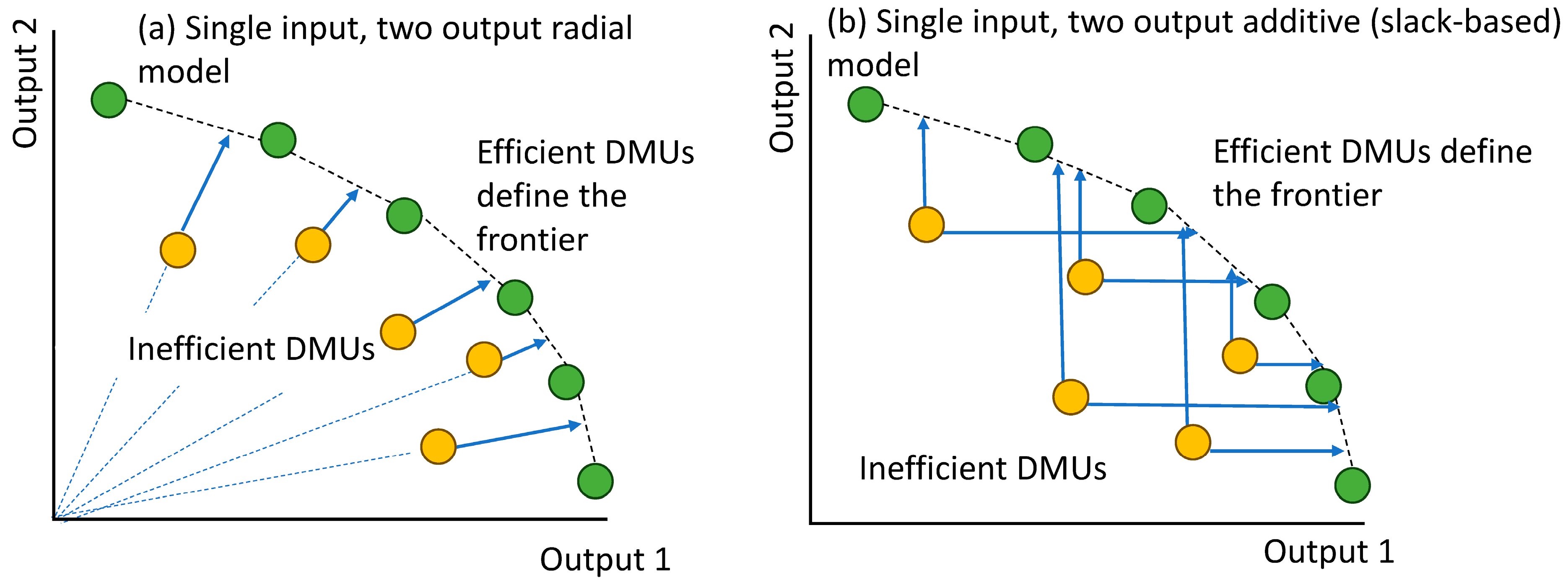
We consider two approaches to the estimation of the management option ‘efficiency’: an output-oriented radial DEA model [24] and an output-oriented additive model (often referred to as a slacks-based model) [25,32,33]. A simplified comparison of the two approaches is given in Figure 1, where the radial model results in a radial expansion to the frontier, while the additive model estimates the horizontal or vertical distance to the frontier. The radially (or additive) expanded inefficient DMU at the frontier may fall between two (or more in the case of multiple outputs) other DMUs (as seen in Figure 1), the position determined by the weighted average of the outputs of the efficient DMUs.

The radial DEA model has been applied in a wide range of contexts, including to assess different management options given multiple objectives [18]. For the purposes of using DEA as an MCDA tool, we employ an output-oriented model as we seek to identify the management options that maximize the outcomes with respect to the multiple objectives or criteria. We can define the output-oriented radial model as:

$$\begin{gathered} Max{\mathsf{\Phi }}_1\mathrm{Subject}\mathrm{to} \\ {\mathsf{\Phi }}_1{y}_{1,m}\le {\displaystyle \sum _j{z}_j{y}_{j,m}}m\in M \\ {\displaystyle \sum _j{z}_j{x}_{j,n}}\le x_{1,n}n\in N \end{gathered}$$

(1)

where ${\mathsf{\Phi }}_1$ is a scalar showing by how much the outcomes of each DMU can increase output, y_j,m is the outcome against objective m by DMU j, x_j,n is amount of input n used by the DMU j (set at 1 for all DMUs) and z_j are weighting factors. In a productivity context, we can add an additional constraint, ${\displaystyle \sum _j{z}_j}=1$, to imposes variable returns to scale in the model; otherwise, the model (implicitly) imposes constant returns to scale. With a single (constant) input, there is no difference between imposing variable returns or constant returns to scale [34]. With variable inputs (e.g., costs of each option), imposing variable returns to scale as well as constant returns to scale may (via the derived measure of scale efficiency) provide additional information to assist decision makers. However, assuming decision makers aim to maximize the outcomes given the available resources, constant returns to scale may be a more appropriate assumption.

From this, the technical efficiency (TE) associated with the management option can be given by:

$$TE=y•{({\mathsf{\Phi }}_{1}y)}^{-1}={{\mathsf{\Phi }}_1}^{-1}$$

(2)

The measure of TE ranges from zero to 1, with 1 being full efficiency (i.e., on the frontier). Values less than 1 indicate that the DMU is operating at less than its full potential given the set of inputs. In the context of our analysis, the most efficient management option is that which best achieves the overall set of objectives.

In this study, we also consider an additive (also known as slacks-based) form of the DEA model, following Tone [25] given by:

$$\begin{gathered} Min{S}_1=\left(\frac{1-(1/n){\displaystyle {\sum }_{i=1}^n{s}_i^{-}}/x_{i0}}{1-(1/m){\displaystyle {\sum }_{j=1}^m{s}_j^{+}}/y_{j0}}\right) \\ {y}_{m0}={\displaystyle \sum _j{z}_j{y}_{j,m}-s_{1,m}^{+}}m\in M \\ {x}_{n0}={\displaystyle \sum _j{z}_j{x}_{j,n}}+s_{1,n}^{-}n\in N \end{gathered}$$

(3)

where the y and x variables are as defined previously, with $s_{1,m}^{+}$ and $s_{1,n}^{-}$ representing the slack variables required to reach the frontier. As with the radial model, adding an additional constraint ${\displaystyle \sum _j{z}_j}=1$ imposes variable returns to scale in the model while excluding this constraint results in constant returns to scale being (implicitly) imposed.

As all DMUs have the same input level, $s_{1,n}^{-}=0 \forall n$ and the objective function can be re-expressed as [35]:

$$Min{S}_1=1-(1/m){\displaystyle {\sum }_{j=1}^m{s}_j^{+}}/y_{j0}$$

(4)

In this case, technical efficiency is given by $T{E}_j^s=0\le S_j\le 1$. A further feature of the measure is that $T{E}_j^s\le T{E}_j$. That is, the slacks-based measure of efficiency is always less than or equal to the radial measure.

The radial models were implemented using the Benchmarking [36] package in R [37], and the slacks-based model using deaR [38].

2.2. Hierarchical Structure of Decision Making

MCDA approaches originate from different theoretical traditions, but most involve some form of aggregation model to allow preference estimates to be combined and compared across criteria [39]. This is generally achieved through the construction of an objective or criterion hierarchy, with specific measurable objectives/criteria [27].

An example of such a hierarchy is given in Figure 2, in which three objectives have a different number of indicators (or measurable sub-objectives) associated with each. In this example, ignoring the hierarchical structure and comparing all indicators at the same time will implicitly give more weight to Objective 3 (as it has the most indicators) and least weight to Objective 2 (as it has the fewest associated indicators).

The hierarchical structure is taken into account in the analysis through first estimating the efficiency score for each objective separately (based on the indicator values that make up that objective), then estimating the overall score using the individual objective scores as the measures. This two-stage process compensates for different objectives having different numbers of indicators when preferences relating to each indicator are unknown.

2.3. Data and Analyses

The analysis utilized two different data sets to test the implications of model choice given the structure of the data used and the importance of hierarchical structures. First, a hypothetical data set was generated to ensure a wide spread of criterion outcomes. The ‘efficiency’ of each set of outcomes was compared given different hierarchical structures and model type (i.e., radial or slacks-based) to assess how these impact the overall scores.

Second, a waste management data set from a previous MCDA application was re-examined using the two different DEA methods, with the DEA outcomes compared with the original MCDA analysis.

The two data sets differ in terms of the relationship between the variables. The variables, representing outcome indicators, within the hypothetical data set are relatively uncorrelated. In contrast, the outcome variables in the waste management data set were more correlated.

A hierarchical structure was also applied to both data sets to test the effects of introducing such a structure on the overall management alternative efficiency score. In the case of the hypothetical data set, this structure was varied to test the effects of different number of indicators/sub-objectives/criteria on the estimated efficiency score and overall estimate of performance. For the waste management data set, the indicators naturally grouped into environmental, technological and economic higher order groups.

2.3.1. Hypothetical Data and Analysis

One hundred DMUs were randomly generated with each producing nine outputs (i.e., indicators) with a range of values from 1 to 10. The R code used to generate and analyze the data is presented in the Supporting Information. The range of values of each variable and the correlation between these values is illustrated in Figure 3. Correlation between the variables was low, generally less than +/−0.2.

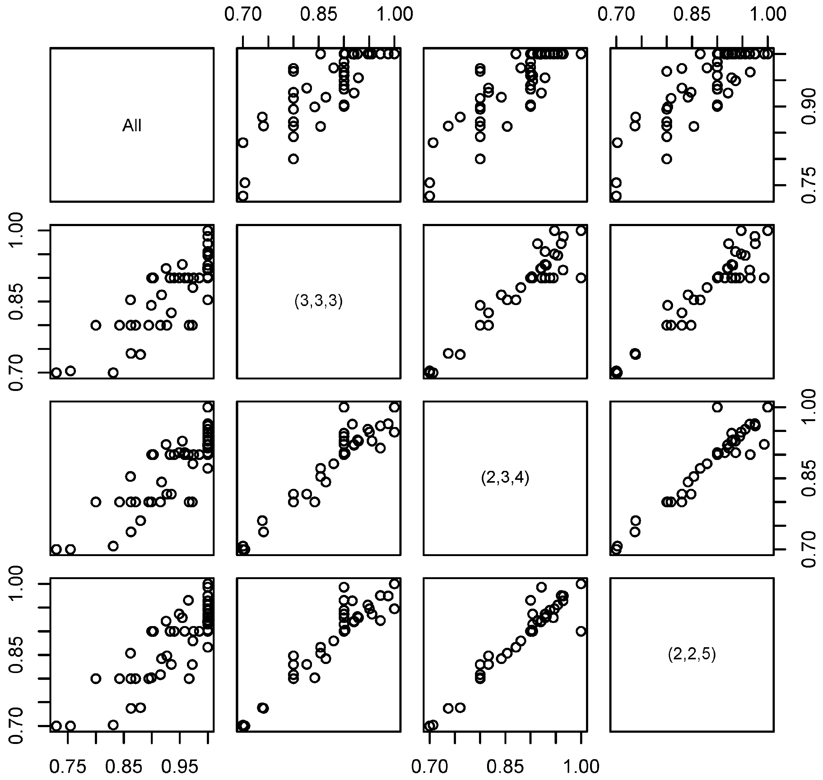
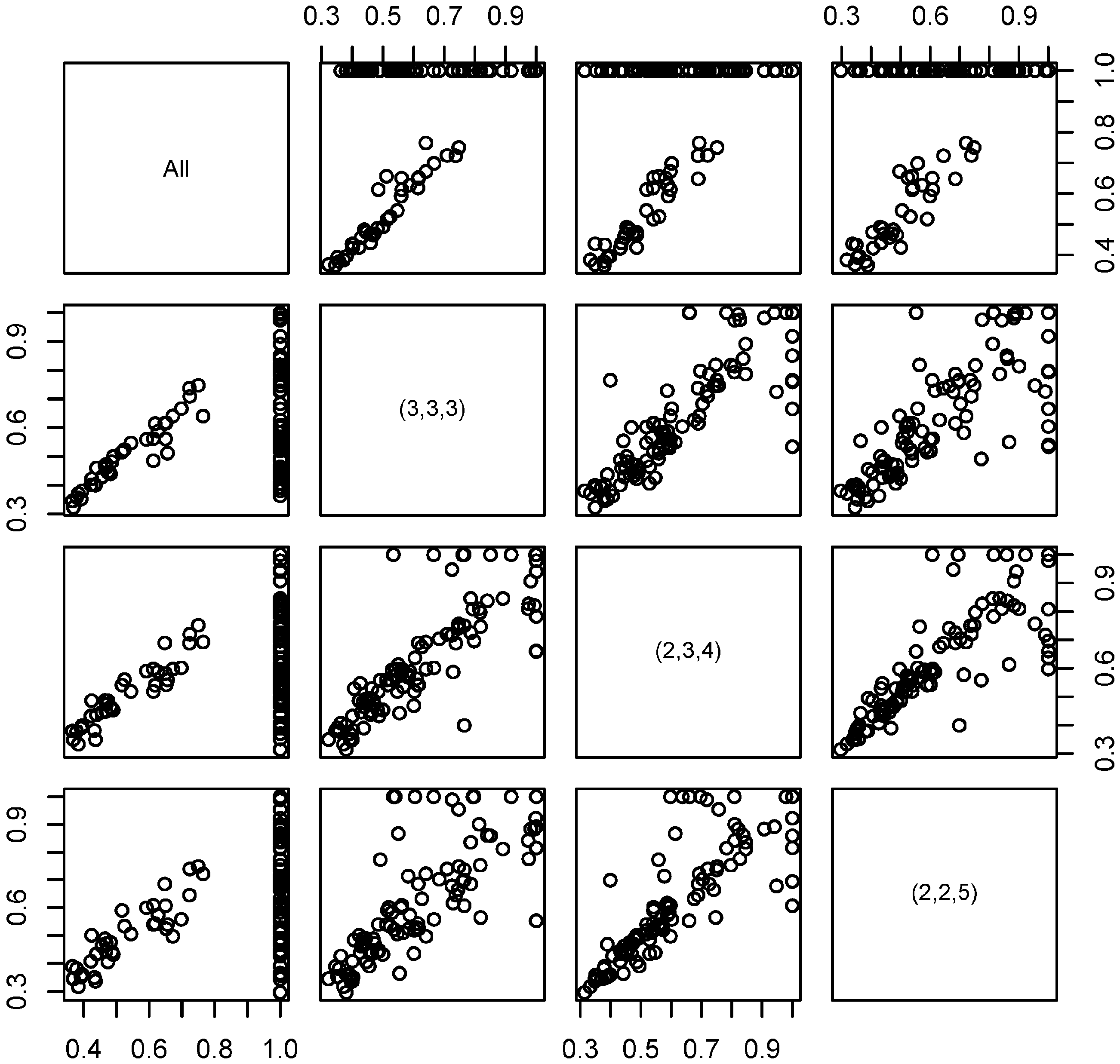
The data were analyzed first by comparing all indicators together using both DEA methods (i.e., radial and slacks-based), and the set of efficient DMUs were identified, representing the management options that produce the greatest overall benefits. A set of different hierarchical structures was then developed. Each structure was assumed to include three different broader ‘objectives’, each with varying numbers of associated indicators. An outline of the experimental design is given in

Table 1. Experimental design used in the hypothetical analysis.

Scenario	Structure	Variables in Each Group
All indicators	9 individual indicators	V1–V9
Hierarchy
Equal	(3, 3, 3)	V1–V3; V4–V6; V7–V9
Unequal	(2, 3, 4)	V1–V2; V3–V5; V6–V9
Very unequal	(2, 2, 5)	V1–V2; V3–V4; V5–V9

, where the number in brackets represents the number of indicators associated with each of the three objectives. The same experimental design was applied to both DEA model types.

For the hierarchical analysis, a two-step process was implemented. First, the indicators within each broader (higher-level) objective were compared first giving an efficiency score for each objective. For example, in the ‘equal’ scenario (Table 1), the efficiency score for the first higher-level objective group was derived using only variables one to three; the second using variables four to six; and the third using variables seven to nine. Next, these higher-level objective group efficiency scores were used as the outcome associated with each broader objective, and the three objectives were compared in a second round of analysis. That is, the efficiency score of each of the higher-level objective group was used as the output, which was then compared with the efficiency score of the other higher order objective groups. The number of indicators associated with each of the broader objectives was changed to see the effects of this on the resultant efficiency score of each DMU.

2.3.2. Waste Management Data

The analysis was also applied using data from a previous MCDA analysis involving a range of different options for development of a waste management system. For each management alternative, a measure of the cost of its implementation and the outcomes in terms of environmental impacts and benefits were estimated. The data were originally produced by Hokkanen and Salminen [40], who applied ELECTRE III [41] to assess the different options, and more recently used by Sarkis [42], who compared DEA to a range of other MCDA approaches.

The data include several undesirable outputs. There are a number of ways of dealing with undesirable outputs, including ignoring them, including them as inputs, or transforming the variables [43]. Sarkis [42] included these undesirable outputs as inputs, along with the costs of their implementation. In our study, we have applied the approach developed by Seiford and Zhu [44], where the undesirable outputs (y) are transformed as y′ = −y + D, where D is a constant value that makes the resultant transformed output (y’) positive for all y. In this case, the maximum value of each of the undesirable variables plus one was added to the negative values. The ‘plus one’ was added such that the minimum value of the transformed variable was 1 (rather than zero). The higher the value of the transformed variable, the better the option compares to the worst performing option. This approach was adopted as the resultant data can be readily applied in both a radial and slacks-based DEA.

The transformed data are presented in

Table 2. Transformed data used in the waste management example.

Alternative	Cost (Input)	Environmental				Technical Reliability	Economic
		Greenhouse Gases	Toxins	Acidic Gases	Nitrogen		Emploment	Waste Recovery
1	656	16.996	62	50	13	5	14	13,900
2	786	30.561	96	50	1	4	18	23,600
3	912	89.109	1	18	89	4	24	39,767
4	589	9.893	260	49	240	9	10	13,900
5	706	37.388	346	49	279	7	14	23,600
6	834	99.061	171	14	299	6.5	18	40,667
7	580	8.686	273	49	263	9	10	13,900
8	682	37.449	357	49	290	7	14	23,600
9	838	103.080	170	11	310	6.5	22	41,747
10	579	8.118	298	49	278	9	9	13,900
11	688	37.372	379	49	313	7	13	23,600
12	838	104.318	172	10	322	6.5	17	42,467
13	595	9.174	171	49	145	9	12	13,900
14	709	36.700	269	49	194	7	17	23,600
15	849	95.537	23	14	145	6.5	20	40,667
16	604	9.174	171	49	145	9	12	13,900
17	736	36.700	269	49	194	7	17	23,600
18	871	95.537	23	14	145	6.5	20	40,667
19	579	1	176	47	125	9	7	13,900
20	695	32.737	247	45	148	6	18	23,600
21	827	112.490	20	3	170	7	16	45,167
22	982	112.468	20	1	170	7	16	45,167

for the 22 different management alternatives. A hierarchy containing three higher-level criteria (Environmental, Technical, and Economic) was assumed and the outputs allocated accordingly. All Environmental outputs were undesirable, with the values in Table 2 being transformed as indicated above. The cost of each management alternative was used as the input.

This is a relatively small data set for use in DEA. To ensure appropriate degrees of freedom in the analysis, the number of comparisons generally should be greater than max[3(m + n), m × n], where m and n are the number of outputs and inputs respectively [45], suggesting that 24 or more comparisons would produce more reliable results. However, fewer alternatives may incorrectly increase the share of fully efficient options (i.e., TE = 1).

Unlike the hypothetical data, the waste treatment data are more highly correlated (

Table 3. Correlation between the transformed variable values in the waste treatment data.

	Greenhouse Gas	Toxins	Acidic Gases	Surface Water Nitrogen	Technical Reliability	Employment	Resource Recovery
Greenhouse gas	1.000
Toxins	−0.570	1.000
Acidic gases	−0.958	0.673	1.000
Surface water nitrogen	0.157	0.633	−0.108	1.000
Technical reliability	−0.468	0.437	0.306	0.416	1.000
Employees	0.746	−0.498	−0.607	−0.152	−0.786	1.000
Resource recovery	0.995	−0.559	−0.944	0.138	−0.493	0.765	1.000

), both positively and negatively. This indicates a greater degree of proportionality in outputs as well as explicit trade-offs (e.g., greenhouse gases compared with acidic gases). This may affect the efficiency scores derived using the different methods.

As with the hypothetical data, the alternatives were examined using both the radial and slacks-based models, and with and without a hierarchical structure imposed.

3. Results

3.1. Using Hypothetical Data

Using the radial model, 66 DMUs were found to be fully efficient when using all indicators together (

Table 4. Number of efficient (TE = 1) DMUs in each scenario.

Scenario	Radial	Slacks-Based
All indicators	66	34
Hierarchy
Equal (3,3,3)	49	6
Unequal (2,3,4)	49	2
Very unequal (2,2,5)	48	10
All scenarios	48	0

). The number of efficient DMUs declined when the hierarchical structure was imposed. Overall, only 48 DMUs were estimated to be efficient across all scenarios, indicating that some treatments suggested that a DMU was efficient, while others suggested that it was not efficient. All three hierarchical treatments produced similar numbers of efficient DMUs, even though the number of indicators compared within each of the broader objectives varied. Forty-eight DMUs were found to be fully efficiency in all cases.

In contrast, the slacks-based model found only 34 fully efficient DMUs, and this number decreased to between two and ten when a hierarchical structure was imposed. In contrast to the analysis using the radial model, no single DMU was found to be fully efficient under all treatments. That is, the results are sensitive to how the variables are distributed between each higher order criterion.

The relative ranking of the outcomes was sensitive to the type of model used as well as how the model was applied (

Table 5. Spearman’s rank correlations between different treatments.

	Radial Model				Slacks-Based Model
Model	All	3,3,3	2,3,4	2,2,5	All	3,3,3	2,3,4	2,2,5
Radial
All	1.000	0.821	0.858	0.841	0.785	0.446	0.441	0.450
3,3,3	0.821	1.000	0.964	0.976	0.628	0.470	0.438	0.435
2,3,4	0.858	0.964	1.000	0.975	0.687	0.439	0.379	0.378
2,2,5	0.841	0.976	0.975	1.000	0.656	0.472	0.417	0.416
Slacks-based
All	0.785	0.628	0.687	0.656	1.000	0.422	0.395	0.430
3,3,3	0.446	0.470	0.439	0.472	0.422	1.000	0.878	0.829
2,3,4	0.441	0.438	0.379	0.417	0.395	0.878	1.000	0.884
2,2,5	0.450	0.435	0.378	0.416	0.430	0.829	0.884	1.000

). The DMU rank using all the indicators was reasonably correlated between the outputs of the two different models, but the rank correlation declined when a hierarchy approach was adopted (and how many indicators were associated with each higher-level objective in the hierarchy). Ranks rather than efficiency scores were compared, as the ordering of the management options (DMUs) is of more relevance to decision analysis.

The outcomes are also compared in Figure 4 and Figure 5 for the radial and slacks-based model respectively. These figures present the distribution of efficiency scores of each treatment against each other treatment.

For both model types, using all indicators separately in the analysis (i.e., the ‘All’ category in Figure 4 and Figure 5) results in a greater proportion of options being identified as fully efficient (i.e., TE = 1), with many of these values being less than 1 when the indicators are split into sub-groups and assessed as a hierarchy.

The value of the efficiency score is also dependent on how the hierarchy is structured, i.e., whether equally balanced across the objectives or unequally balanced. This is more pronounced for the slacks-based model (Figure 5), where the efficiency scores showed greater differences based on which hierarchy structure was imposed than for the radial DEA model.

3.2. Using the Waste Management Data

The estimated efficiency scores (i.e., cost-effectiveness measures) and their relative rankings are given in

Table 6. Efficiency scores and relative rankings given different estimation procedures.

Alternative	Efficiency Scores				Rank of Efficiency Scores
	Radial		Slacks-Based		Radial		Slacks-Based
	All	Hierarchy	All	Hierarchy	All	Hierarchy	All	Hierarchy
1	0.984	0.934	0.268	0.242	16	9	20	19
2	0.931	0.797	0.025	0.023	20	18	21	21
3	1.000	0.774	1.000	0.028	1	18	1	20
4	0.996	0.977	0.961	0.941	13	6	11	5
5	0.966	0.831	0.955	0.766	15	14	11	11
6	0.998	0.827	0.953	0.686	12	14	11	12
7	1.000	1.000	1.000	1.000	1	1	1	1
8	1.000	0.891	1.000	0.921	1	7	1	4
9	1.000	0.863	1.000	0.914	1	10	1	4
10	1.000	1.000	1.000	1.000	1	1	1	1
11	1.000	0.864	1.000	0.830	1	8	1	4
12	1.000	0.833	1.000	0.689	1	8	1	6
13	1.000	1.000	1.000	1.000	1	1	1	1
14	1.000	0.943	1.000	0.823	1	4	1	3
15	0.971	0.805	0.414	0.405	5	6	6	6
16	0.985	0.970	0.923	0.796	4	3	3	3
17	0.963	0.875	0.919	0.681	4	4	3	3
18	0.947	0.764	0.382	0.343	4	4	4	4
19	1.000	1.000	0.428	0.430	1	1	3	3
20	1.000	1.000	1.000	0.873	1	1	1	2
21	1.000	0.875	1.000	1.000	1	1	1	1
22	0.842	0.621	0.179	0.149	1	1	1	1

. Both the radial and slacks-based approach estimated that more alternatives were efficient when all data were compared than when the hierarchical structure of the information was taken into consideration. For example, the number of efficient (i.e., TE = 1) alternatives using all data was found to be 12 and 11 for the radial and slacks-based model respectively, decreasing to 5 and 4 alternatives when the hierarchical structure was imposed.

The relative rankings also changed substantially when the hierarchical structure was imposed. For example, alternative 3 was found to be efficient (TE = 1; rank = 1) when all the data were used, although it fell to 18th and 20th place, respectively, when the hierarchical structure was imposed (Table 6).

The efficiency scores also differed substantially for several of the alternatives when estimated using the different models. For example, the efficiency scores for alternative 2 were substantially lower when estimated using the slacks-based model than the radial model, although the impact of this on their rank was less pronounced.

The correlations between the ranks from the different measures are presented in

Table 7. Rank correlations between different models, waste management example.

	Electre III	Radial DEA		Slacks-Based Model
		All	Hierarchy	All	Hierarchy
ELECTRE III	1.000
Radial all	0.369	1.000
Radial Hierarchy	0.228	0.405	1.000
SBM all	0.510	0.907	0.356	1.000
SBM Hierarchy	0.621	0.509	0.762	0.627	1.000

. Hokkanen and Salminen [40] provided the relative rankings of each of the option using the ELECTRE III method, and these are also included in the correlation matrix in Table 7. The correlation between ELECTRE III and the ranks derived using DEA were generally low, but were higher for the slacks-based model in general and for the hierarchical slacks-based model in particular. The ELECTRE III method incorporates preference weights for the different criteria, although unfortunately these weights were not presented by the authors [40].

4. Discussion

The underlying use of hierarchical structures in MCDA is relatively common. Different management objectives often have a different number of sub-objectives, or a different number of indicators relating to each objective. Introducing a hierarchical structure in the assessment of management alternatives using DEA provides a number of benefits. Foremost, it allows an assessment of how each management alternative relates to each objective as an overall benefit of the doubt measure over all objectives and indicators. While not considered in this study, the efficiency score associated with each group of indicators (i.e., potentially representing a separate management objective) could be considered as well as the overall performance measure of the management option.

The use of an intermediate step also has benefits in terms of saving degrees of freedom when data are limited. The number of indicators that can be compared in an analysis is limited by the number of available observations. The discrimination power and accuracy of DEA with respect to the ability to estimate the performance of DMUs decreases as the number of DMUs decreases or the numbers of inputs and outputs increases [46]. While there is no definitive estimate of the number of observations required to ensure robust estimation of the efficiency scores, a commonly applied rule of thumb is that the number of observations (DMUs) should be greater than max[3(m + n), m × n], where m and n are the number of outputs and inputs, respectively [45]. In our hypothetical example, with nine outputs and one input, 30 observations would be required to meet this. With 100 generated DMUs, this was not a concern. For the waste management example, however, degrees of freedom issues may have contributed to the large number of efficient alternatives when all the data were used, but substantially fewer when breaking the problem up into essentially four separate estimation stages (one each for each objective and one for the combined objective level analysis). For example, when all data were used, the problem required 24 observations (i.e., 3 × (7 + 1) alternatives) although only 22 alternatives were available. In contrast, estimating the efficiency score associated with just the environmental objectives required only 15 observations (i.e., 3 × (4 + 1)).

If decision makers do have differing preferences for the different objectives, then weights can be applied also at each stage to provide a weighted overall efficiency score. While not explicitly covered in this study, an example of how importance weights can be applied in DEA is given by Pascoe et al. [18]. If weights were available for the waste management example, it is expected that the correlation between the MCDA and DEA model rankings would have been greater.

In the hypothetical analysis, each observation was treated as a separate management option for consideration. In many MCDA studies, multiple sets of observations are associated with each management option reflecting uncertainty in management outcomes. These may be derived through stochastic simulation using models or through (differing) expert opinion from a range of experts. The DEA framework offers particular advantages in this case, as each potential outcome set is compared with all other sets. The resultant efficiency scores can be considered as a distribution associated with each management option, allowing the effects of uncertainty to be explicitly captured in the analysis.

We find that the results (i.e., efficiency scores and relative rankings) are also sensitive to model choice. From the results using both data sets, the slacks-based model approach provided greater discrimination between management options (DMUs), with a smaller set of options identified as efficient. Avkiranet al. [35] note a key challenge with radial models is that an identified efficient DMU may still exhibit lower levels of output in some indicators that others that are also identified as efficient. Slacks-based models directly assess these indicator-specific differences, although the loss of the proportionality assumption may mean that the ability of the options to achieve efficiency is limited if such a proportionality constraint exists [35]. However, as we are not interested in improving the efficiency of inefficient management alternatives but identifying which options are the most efficient in a multi-criterion environment then this is not necessarily a problem.

The choice of which model to use to assess the management alternative may depend on the degree of independence between management outcomes. If management outcomes are perfectly independent, such that trade-offs between them are possible, then the slacks-based model may be more appropriate. Conversely, if the outcomes are not totally independent, such that increasing one will require in some increase in another (and vice versa), then the radial model may be more appropriate given the associated proportionality assumptions. In the hypothetical data set, each outcome was total independent, and hence the slacks-based model was able to provide greater discrimination between the hypothetical alternatives that produced them. For the waste management example, several outputs were correlated (e.g., toxins, acidic gases and nitrogen released in the water), suggesting the proportionality approach underlying the radial model may have been appropriate. For the waste management example, both models produced similar rankings and numbers of ‘efficient’ options, with the utilisation of the hierarchical structure more important in distinguishing the most efficient alternatives.

The study assumes that the relative preferences for each of the management outcomes is unknown, and hence the models provide a ‘benefit of the doubt’ measure of the efficiency of the different alternative. Under this scenario, the outcomes are sensitive to what form of model is used and how (if any) hierarchy of criteria is employed. The addition of preference weights is possible in DEA as noted previously, and this may reduce these differences if the importance of each criterion to the decision maker was more explicit. This is an area for future consideration.

5. Conclusions

The results of the analysis have several implications for the use of DEA for MCDA. First, as a ‘benefit of the doubt’ measure, DEA will not necessarily identify a single ‘best’ management option, but may instead identify a subset of efficient options. These options will have different strengths with regard to different objectives. With the addition of objective weightings, this subset may be able to be narrowed further and potentially a single best option identified. Without a set of objective weights, managers will need to assess trade-offs within this (reduced) group subjectively.

Second, in cases where different objectives have a different number of indicators (or quantifiable and measurable sub-objectives), ignoring the implicit (or explicit) hierarchical structure can result in less efficient management options appearing to be efficient. This could result in less-than optimal decisions being made, as the pool of potentially optimal management options is greater than it should be. The triple bottom line framework (i.e., environmental, social and economic) provides a useful conceptual classification system for many MCDA variables, even if an explicit hierarchy has not been pre-determined.

The third key result is that the efficiency scores, and hence ranking of the management options, are sensitive to the DEA approach, with the radial approach potentially overestimating the proportion of efficient options when the outcome data are uncorrelated. In contrast, the slacks-based approach can provide greater discrimination between management options, minimizing the set of efficient options that need to be subsequently considered.