
An Adaptive Linear Programming Algorithm with Parameter Learning
 , , , and
Abstract
1. Introduction
1.1. Frame of Reference
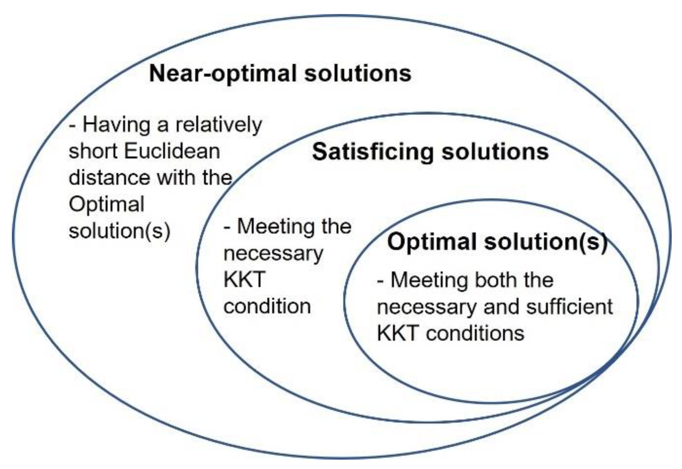
1.2. Mechanisms to Ensure That the cDSP and ALP Find Satisficing Solutions
1.3. An Example and Explanation Using KKT Conditions
1.4. A Limitation in the ALP to Be Improved
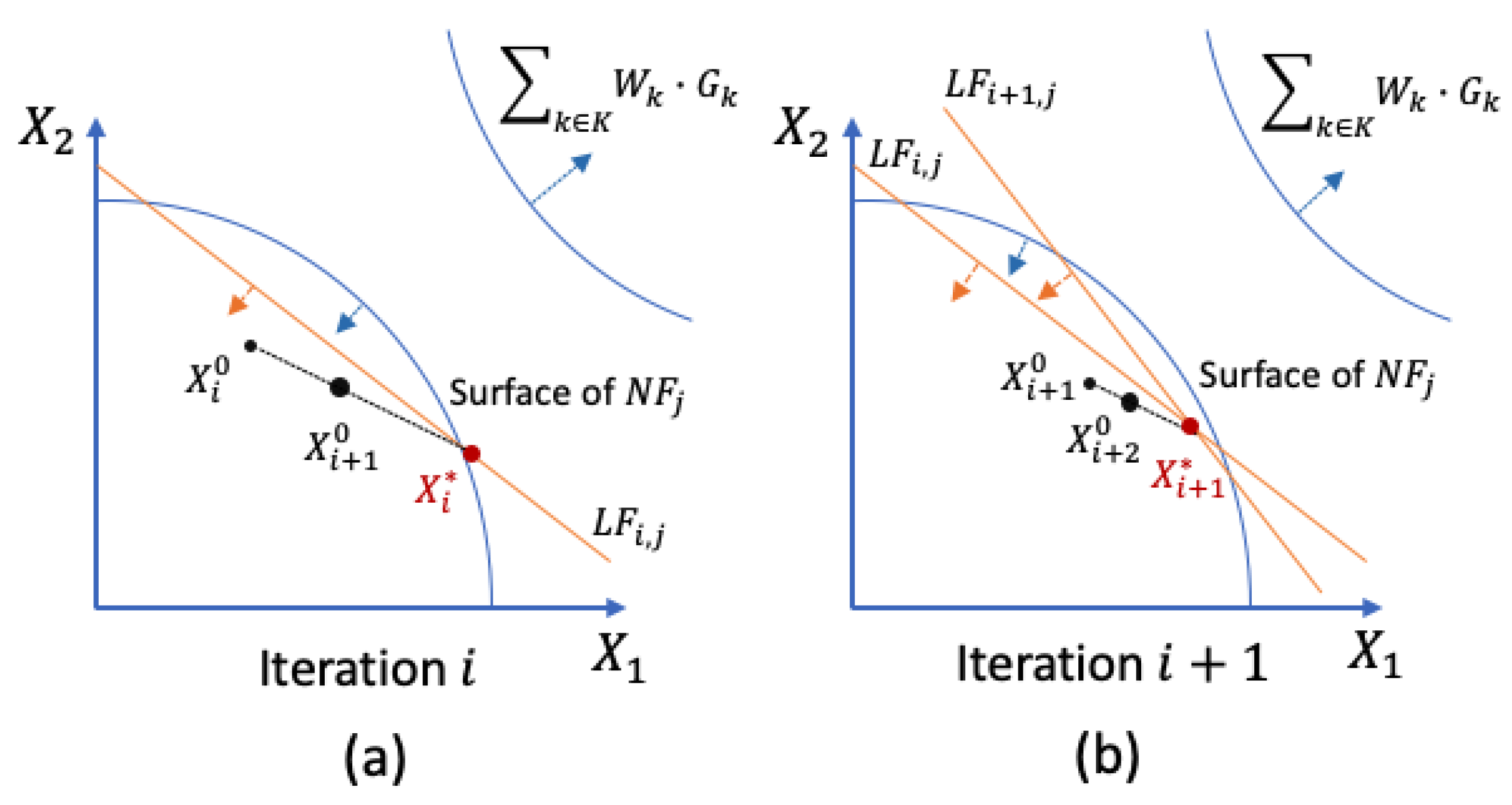
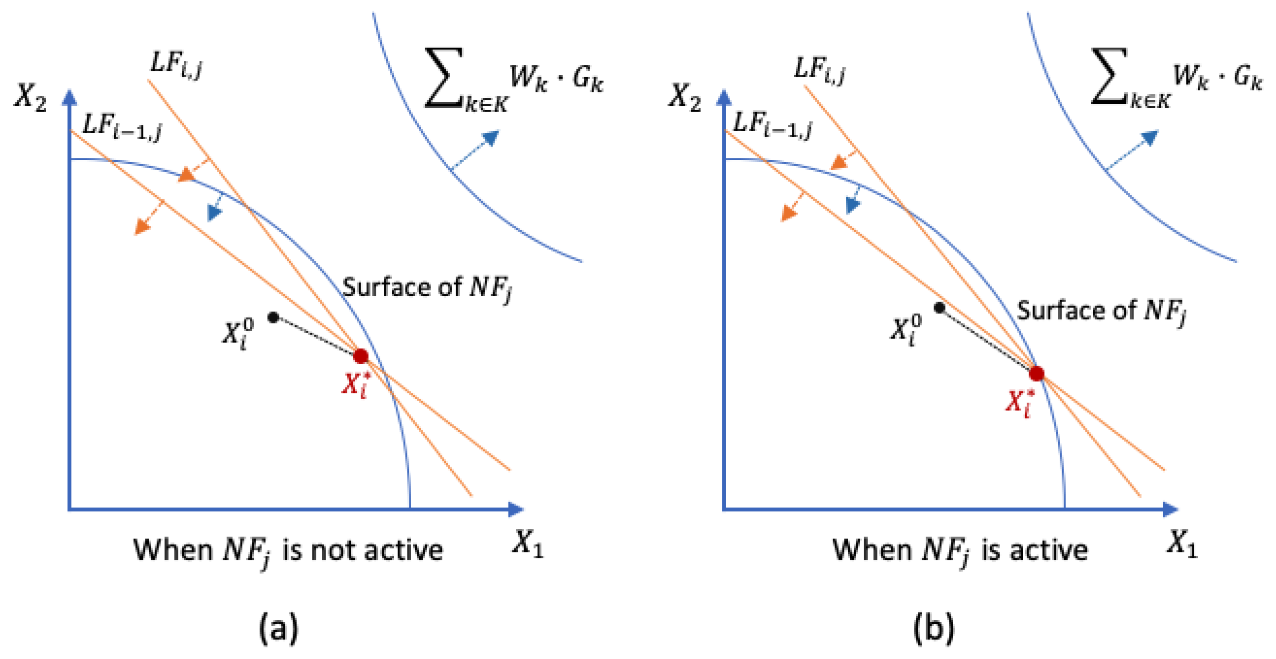
2. How Does the ALP Work?
2.1. The Adaptive Linear Programming (ALP) Algorithm
| Algorithm 1. Constraint Accumulation Algorithm |
| In the ith iteration, for every j in J if and |
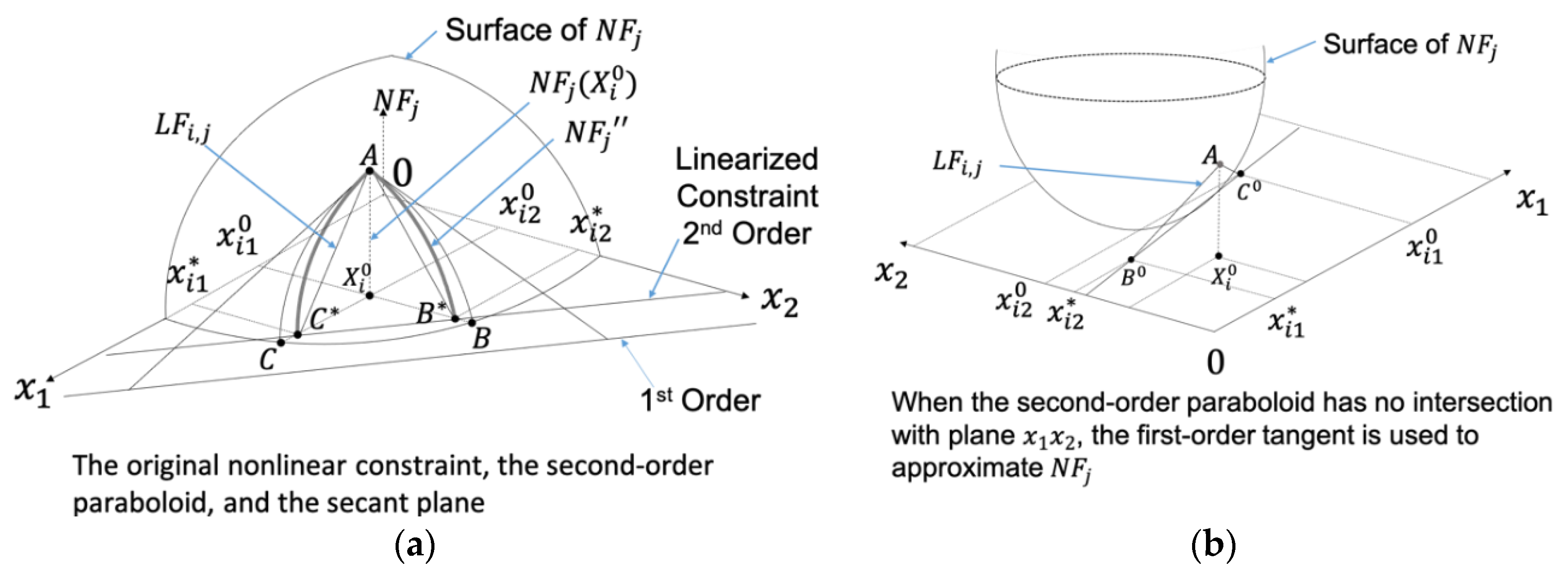
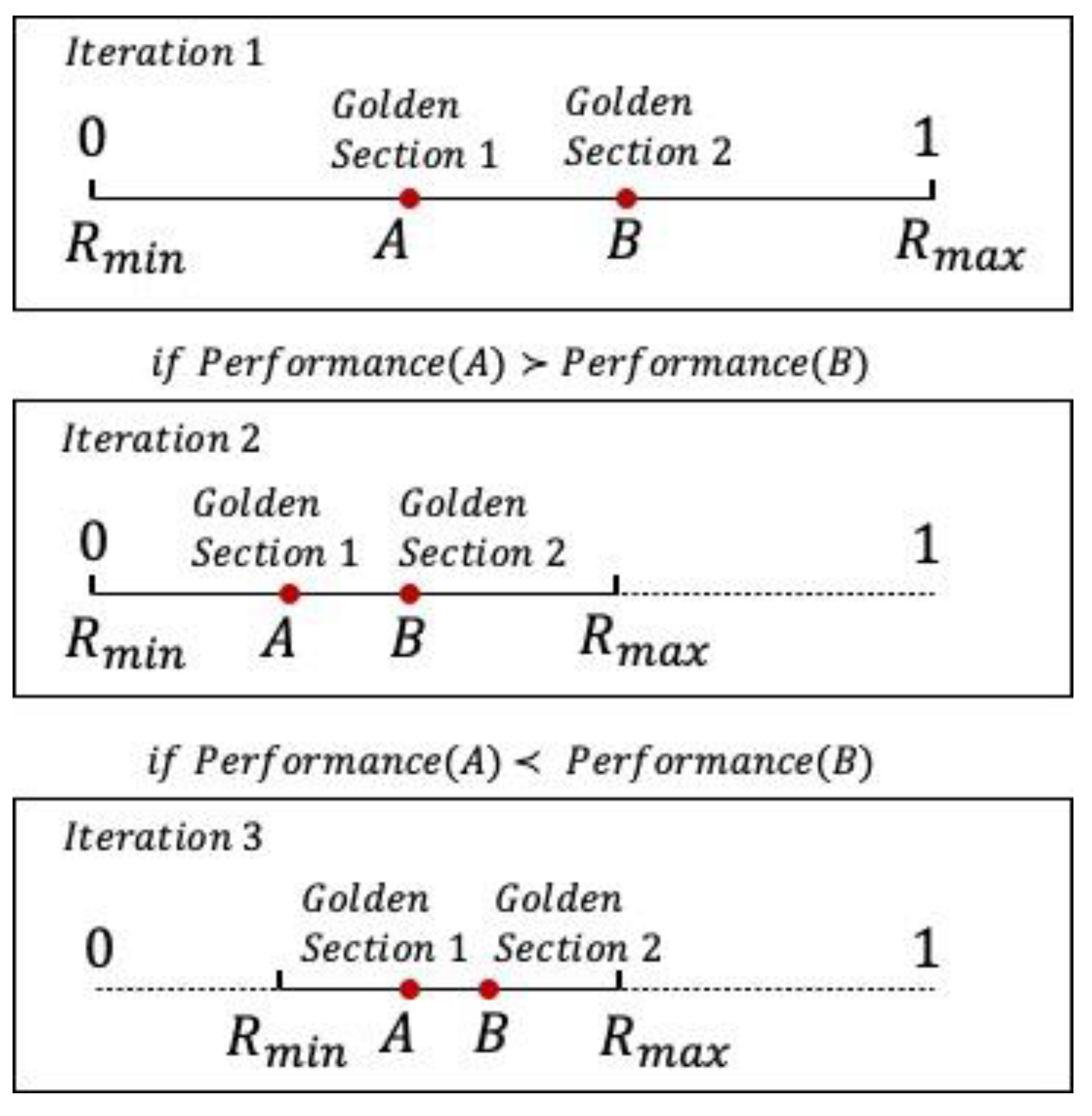
2.2. The Reduced Move Coefficient
| Algorithm 2. Golden section search for updating the RMC |
| #Define Performance function using RMC to linearize the model and obtain the merit function value FUNCTION Performance (Model, RMC) Linearize Model using ALP with RMC into Linear_Model Solve Linear_Model using Dual Simplex RETURN Z #Define Golden Section Search function FUNCTION GoldenSectionSearchForRMC (Rmin, Rmax, Th): RMCa = Rmin + (0.382)*(Rmax − Rmin) RMCb = Rmin + (1 − 0.382)*(Rmax − Rmin) WHILE (RMCb − RMCa > Th): #Compare the performance of using RMCa versus RMCb IF Performance (Original_Model, RMCa) < Performance (Original_Model, RMCb): RMC = RMCa Rmax = RMCb ELSE: RMC = RMCb Rmin = RMCa RETURN RMC #Initialize parameters Rmin = 0 Rmax = 1 Th = 0.0001 #Call the Golden Section Search Function GoldenSectionSearchForRMC (Rmin, Rmax, Th) |
- Step 1. Identifying the criteria—to evaluate approximation performance.
- Step 2. Developing evaluation indices (EIs)—to quantify the approximation performance with RMC values.
- Step 3. Learning the desired range of each EI (DEI)—to tune the RMC.
3. Parameter Learning to Dynamically Change the RMC
3.1. Step 1—Identifying the Criteria
- Criterion 1—deviation.
- Criterion 2—robustness of solutions.
- Criterion 3—approximation accuracy.
3.2. Step 2—Developing the Evaluation Indices (EIs)
| Algorithm 3. #Define Parameter-learning function |
| FUNCTION ParameterLearning(Model, Design scenarios, RMC, EIs, κ, I): WHILE i < I: IF RMC[i-1] = RMC_best: RMC[i] = average(RMC[i-2], RMC_best) ELSE: RMC[i] = average(RMC[i-1], RMC_best) FOR N Design Scenarios: Linearize Model using ALP with RMC[i] into Linear_Model Solve Linear_Model using Dual Simplex RETURN EIs[i] FOR j in Range(0, i): Rank EIs[i][j] from minimum to maximum DEI = EIs[i][round(κ*i)] IF (number of EIs[i] ∈ DEI for all Design scenarios) > (number of EIs[Cycle of RMC_best] ∈ DEI for all Design scenarios): RMC_best = RMC[i] RETURN RMC_best #Initialize parameters Model = Original_Model Design scenarios = N weight scenarios RMC [0] = 0.5 EIs = [μZ, σZ, μNab, σNab, μNaoc, σNaoc, μNacc, σNacc, μNit, σNit] Z, Nab, Naoc, Nacc, Nit = 0 DEI = [0, 0, 0, 0, 0, 0, 0, 0, 0, 0] κ = 0.6 I = 50 #Call Parameter-Learning function FUNCTION ParameterLearning(Model, Design scenarios, RMC, EIs, κ, I) |
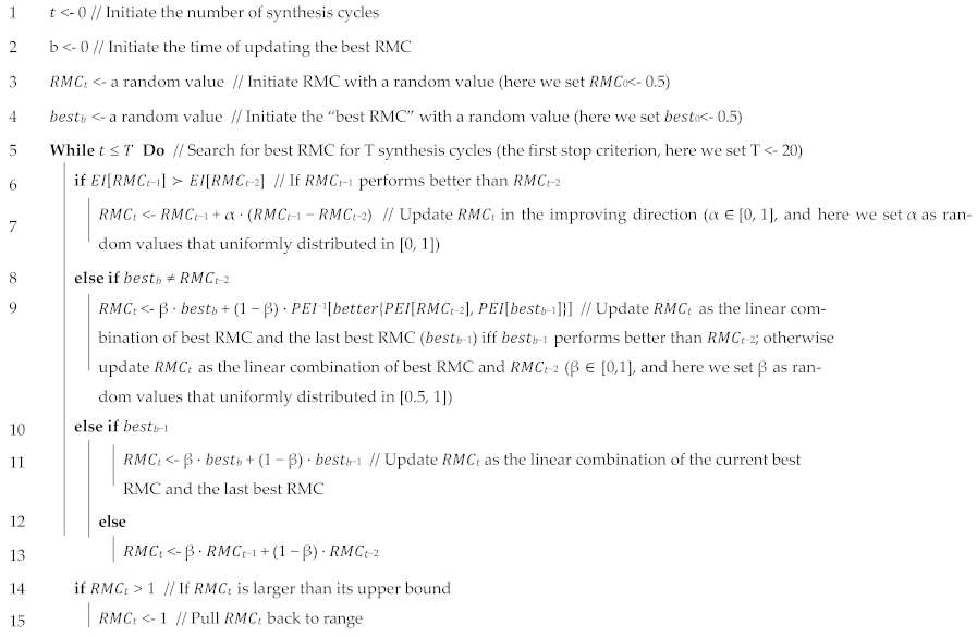
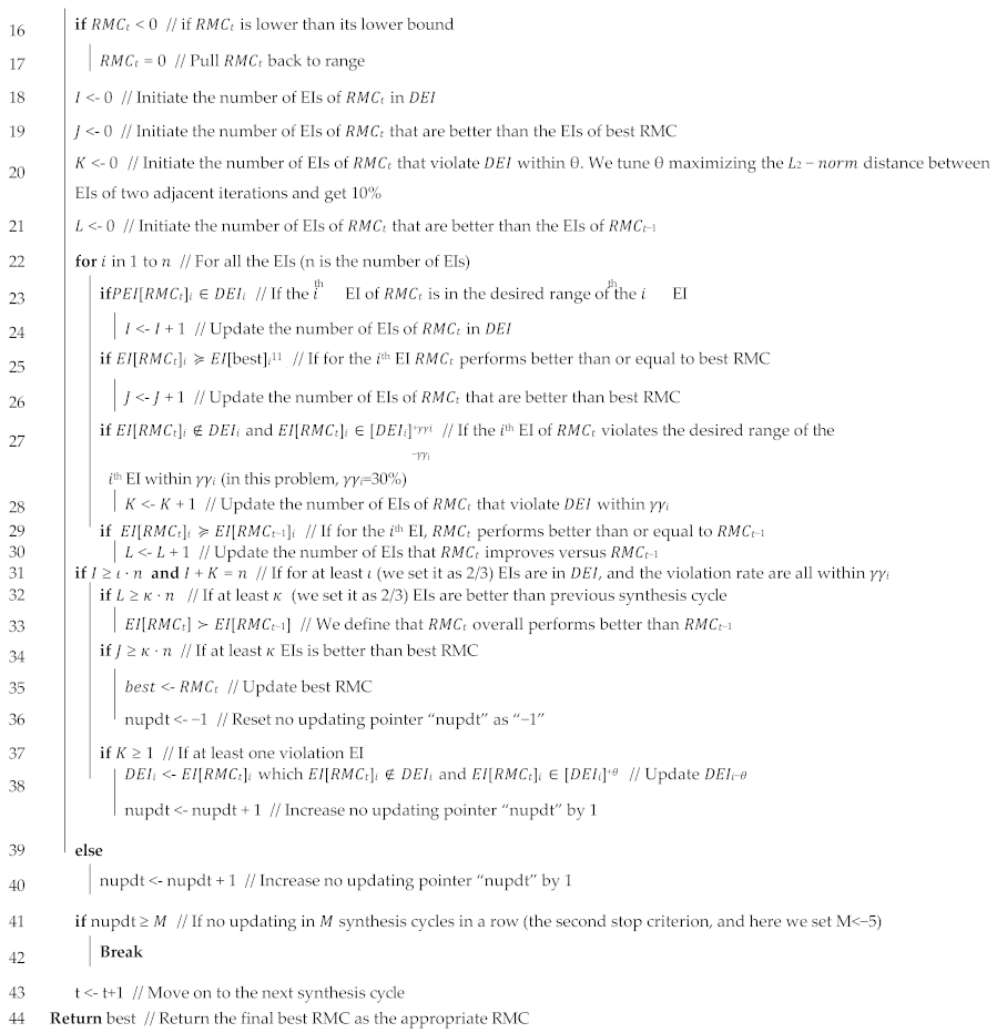
3.3. Step 3—Learning the DEI to Tune the RMC
| Algorithm 4. The RMC parameter-learning algorithm |
| 1 Given: the best RMC sample value, updating rules 2 Initialize: t = 0, best = the best RMC sample value, RMC0 = the best RMC sample value, the maximum iteration number T, stopping criterion 2 = {best has not been updated in n iterations} 3 While t = do T // Define stopping criterion 1 4 RMCt = Next_RMC 5 Run synthesis cycle |
4. A Test Problem
4.1. The Hot Rod-Rolling Process Chain
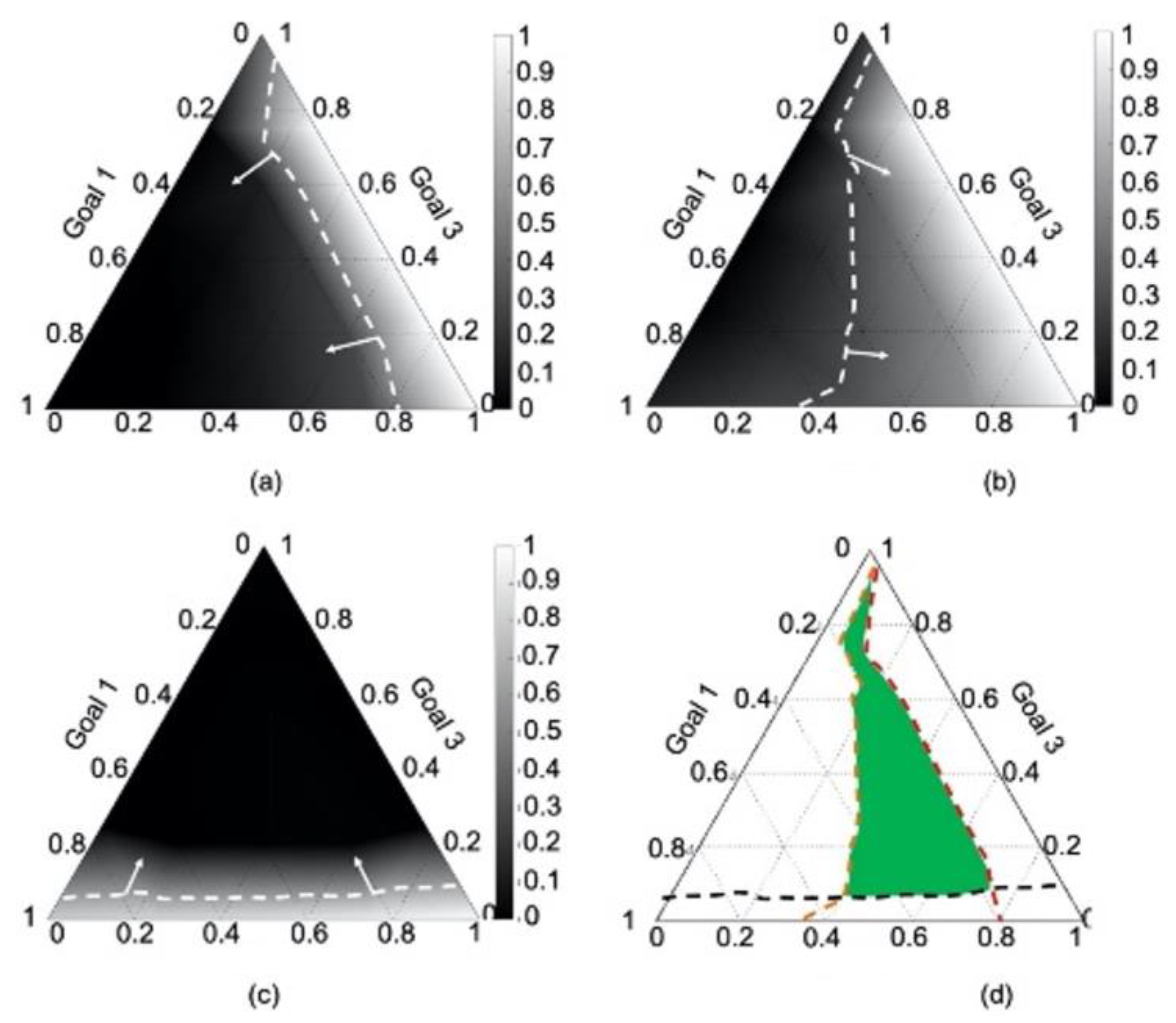
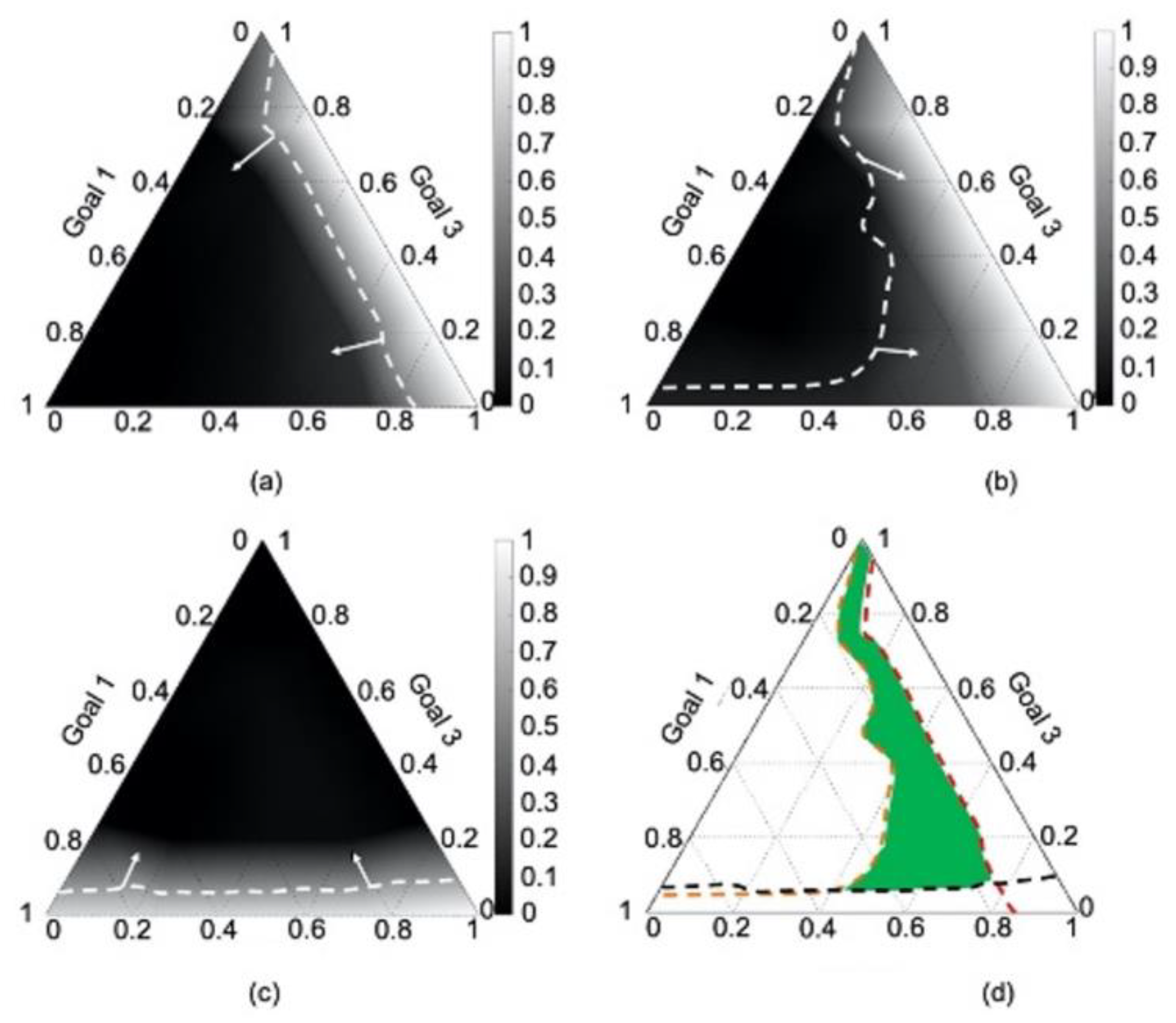
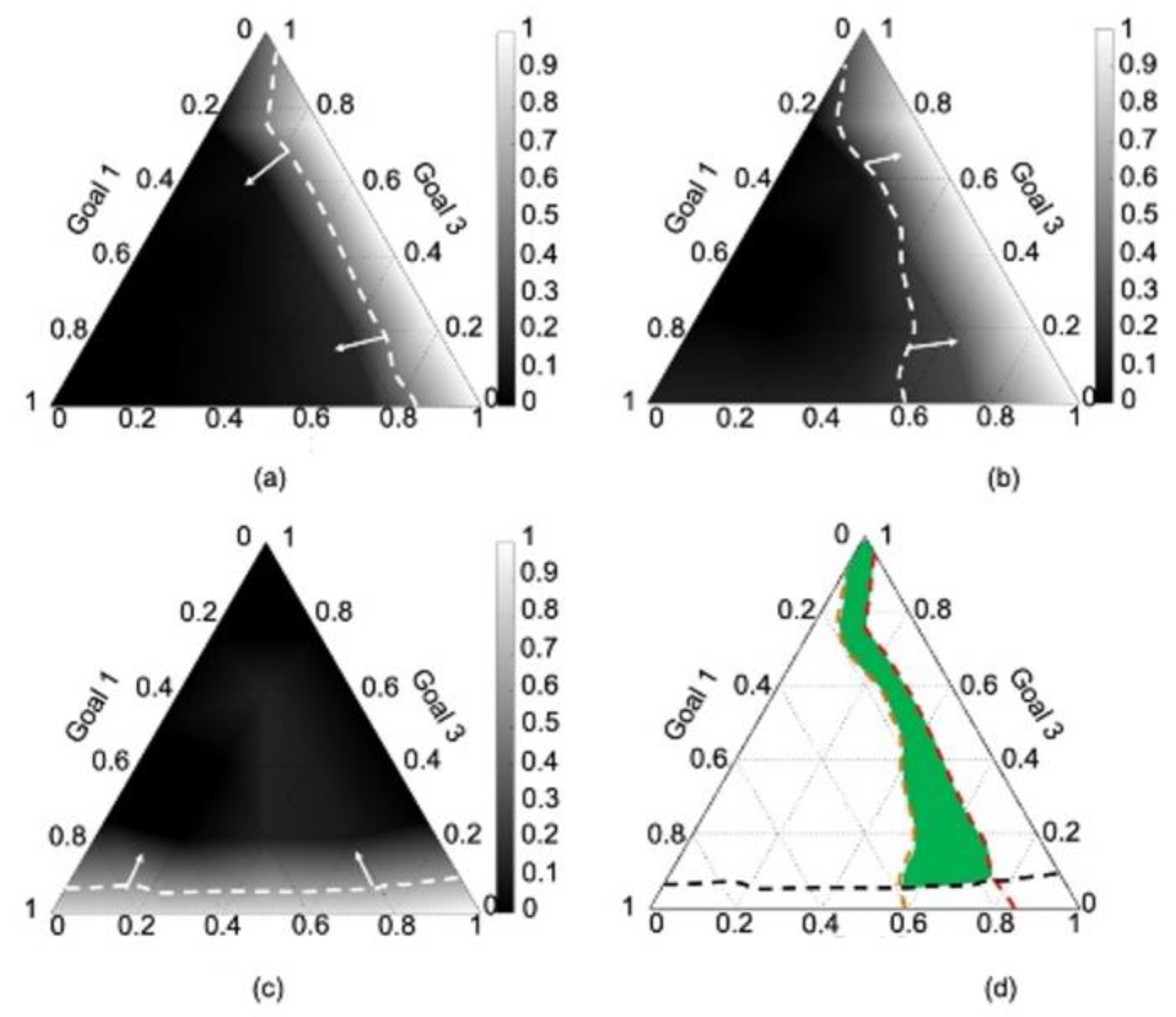
- The range of the system variables to reach the target of each goal of the best RMC for different design preferences and
- The weight set, , that is a compromise of the three goals for different design preferences.
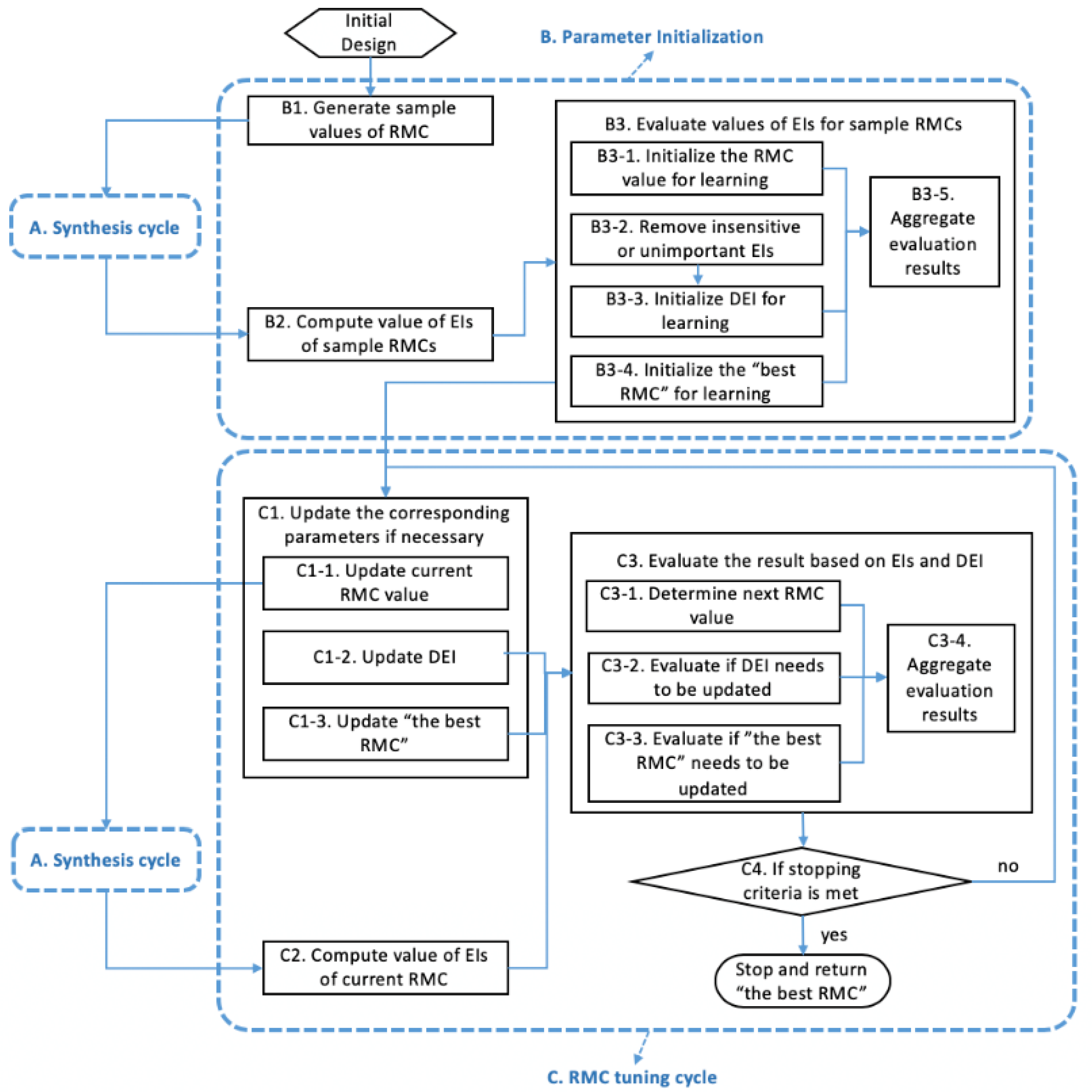
4.2. Parameter Initialization
4.3. RMC Tuning
4.4. Results
4.5. Verification and Validation
5. Closing Remarks
6. Glossary
Author Contributions
Funding
Data Availability Statement
Acknowledgments
Conflicts of Interest
Nomenclature
| ALP | Adaptive Linear Programming |
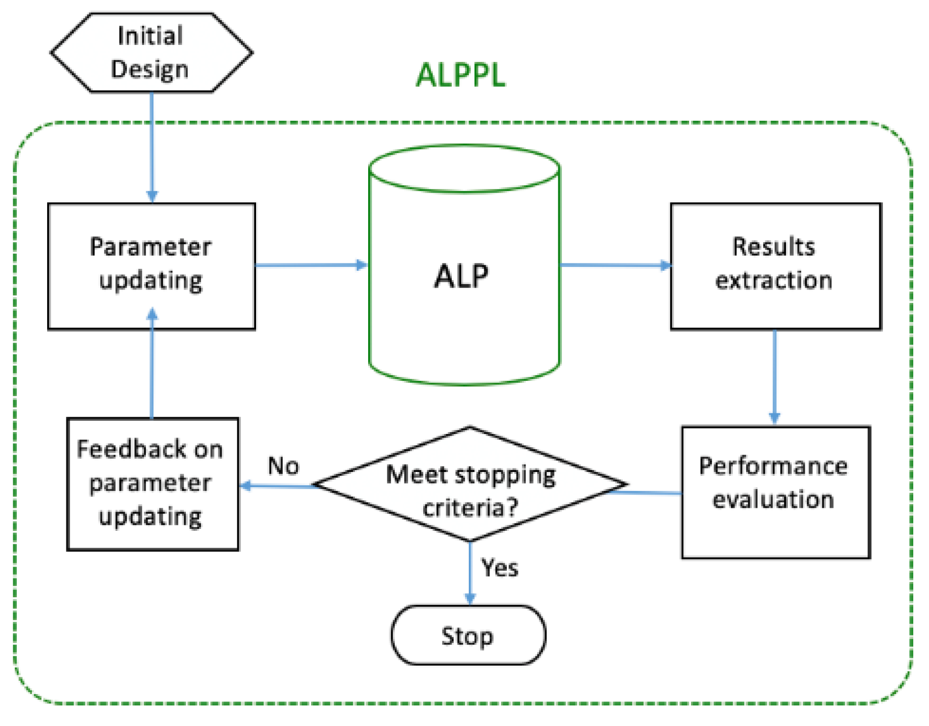
| ALPPL | Adaptive Linear Programming with Parameter Learning |
| cDSP | Compromise Decision Support Problem |
| DEI | Desired Range of Evaluation Index |
| DSP | Decision Support Problem |
| EI/EIs | Evaluation Index/Indices |
| RMC | Reduced Move Coefficient |
Appendix A
The RMC Parameter-Learning Algorithm Customized for the Hot Rolling Process Chain Problem
| Algorithm A1. The RMC parameter-learning algorithm (Algorithm 4) customized for the Cooling Procedure of the Hot Rolling Problem |
  |
References
- Rios, L.M.; Sahinidis, N.V. Derivative-Free Optimization: A Review of Algorithms and Comparison of Software Implementations. J. Glob. Optim. 2013, 56, 1247–1293. [Google Scholar] [CrossRef]
- Vrahatis, M.N.; Kontogiorgos, P.; Papavassilopoulos, G.P. Particle Swarm Optimization for Computing Nash and Stackelberg Equilibria in Energy Markets. SN Oper. Res. Forum 2020, 1, 20. [Google Scholar] [CrossRef]
- Behmanesh, E.; Pannek, J. A Comparison between Memetic Algorithm and Genetic Algorithm for an Integrated Logistics Network with Flexible Delivery Path. Oper. Res. Forum 2021, 2, 47. [Google Scholar] [CrossRef]
- Viswanathan, J.; Grossmann, I.E. A Combined Penalty Function and Outer-Approximation Method for MINLP Optimization. Comput. Chem. Eng. 1990, 14, 769–782. [Google Scholar] [CrossRef]
- Nagadurga, T.; Devarapalli, R.; Knypiński, Ł. Comparison of Meta-Heuristic Optimization Algorithms for Global Maximum Power Point Tracking of Partially Shaded Solar Photovoltaic Systems. Algorithms 2023, 16, 376. [Google Scholar] [CrossRef]
- Mistree, F.; Hughes, O.F.; Bras, B. Compromise decision support problem and the adaptive linear programming algorithm. Prog. Astronaut. Aeronaut. Struct. Optim. Status Promise 1993, 150, 251. [Google Scholar]
- Teng, Z.; Lu, L. A FEAST algorithm for the linear response eigenvalue problem. Algorithms 2019, 12, 181. [Google Scholar] [CrossRef]
- Rao, S.; Mulkay, E. Engineering design optimization using interior-point algorithms. AIAA J. 2000, 38, 2127–2132. [Google Scholar] [CrossRef]
- Asghari, M.; Fathollahi-Fard, A.M.; Al-E-Hashem, S.M.; Dulebenets, M.A. Transformation and linearization techniques in optimization: A state-of-the-art survey. Mathematics 2022, 10, 283. [Google Scholar] [CrossRef]
- Reich, D.; Green, R.E.; Kircher, M.; Krause, J.; Patterson, N.; Durand, E.Y.; Viola, B.; Briggs, A.W.; Stenzel, U.; Johnson, P.L. Genetic history of an archaic hominin group from Denisova Cave in Siberia. Nature 2010, 468, 1053–1060. [Google Scholar] [CrossRef]
- Fishburn, P.C. Utility theory. Manag. Sci. 1968, 14, 335–378. [Google Scholar] [CrossRef]
- Nash, J.F., Jr. The bargaining problem. Econom. J. Econom. Soc. 1950, 18, 155–162. [Google Scholar] [CrossRef]
- Saaty, T.L. What Is the Analytic Hierarchy Process? Springer: Berlin/Heidelberg, Germany, 1988. [Google Scholar]
- Calpine, H.; Golding, A. Some properties of Pareto-optimal choices in decision problems. Omega 1976, 4, 141–147. [Google Scholar] [CrossRef]
- Guo, L. Model Evolution for the Realization of Complex Systems. Ph.D. Thesis, University of Oklahoma, Norman, OK, USA, 2021. [Google Scholar]
- Speakman, J.; Francois, G. Robust modifier adaptation via worst-case and probabilistic approaches. Ind. Eng. Chem. Res. 2021, 61, 515–529. [Google Scholar] [CrossRef]
- Souza, J.C.O.; Oliveira, P.R.; Soubeyran, A. Global convergence of a proximal linearized algorithm for difference of convex functions. Optim. Lett. 2016, 10, 1529–1539. [Google Scholar] [CrossRef]
- Su, X.; Yang, X.; Xu, Y. Adaptive parameter learning and neural network control for uncertain permanent magnet linear synchronous motors. J. Frankl. Inst. 2023, 360, 11665–11682. [Google Scholar] [CrossRef]
- Courant, R.; Hilbert, D. Methods of Mathematical Physics; Interscience: New York, NY, USA, 1953; Volume 1. [Google Scholar]
- Guo, L.; Chen, S. Satisficing Strategy in Engineering Design. J. Mech. Des. 2024, 146, 050801. [Google Scholar] [CrossRef]
- Powell, M.J. An Efficient Method for Finding the Minimum of a Function of Several Variables without Calculating Derivatives. Comput. J. 1964, 7, 155–162. [Google Scholar] [CrossRef]
- Straeter, T.A. On the Extension of the Davidon-Broyden Class of Rank One, Quasi-Newton Minimization Methods to an Infinite Dimensional Hilbert Space with Applications to Optimal Control Problems; North Carolina State University: Raleigh, NC, USA, 1971. [Google Scholar]
- Fletcher, R. Practical Methods of Optimization, 2nd ed.; John Wiley & Sons: Hoboken, NJ, USA, 1987. [Google Scholar]
- Khosla, P.; Rubin, S. A Conjugate Gradient Iterative Method. Comput. Fluids 1981, 9, 109–121. [Google Scholar] [CrossRef]
- Nash, S.G. Newton-type Minimization via the Lanczos Method. SIAM J. Numer. Anal. 1984, 21, 770–788. [Google Scholar] [CrossRef]
- Zhu, C.; Byrd, R.H.; Lu, P.; Nocedal, J. Algorithm 778: L-BFGS-B: Fortran Subroutines for Large-scale Bound-Constrained Optimization. ACM Trans. Math. Softw. (TOMS) 1997, 23, 550–560. [Google Scholar] [CrossRef]
- Powell, M. A Tolerant Algorithm for Linearly Constrained Optimization Calculations. Math. Program. 1989, 45, 547–566. [Google Scholar] [CrossRef]
- Powell, M.J. A View of Algorithms for Optimization without Derivatives. Math. Today Bull. Inst. Math. Its Appl. 2007, 43, 170–174. [Google Scholar]
- Deb, K.; Pratap, A.; Agarwal, S.; Meyarivan, T. A fast and elitist multiobjective genetic algorithm: NSGA-II. IEEE Trans. Evol. Comput. 2002, 6, 182–197. [Google Scholar] [CrossRef]
- Guo, L.; Balu Nellippallil, A.; Smith, W.F.; Allen, J.K.; Mistree, F. Adaptive Linear Programming Algorithm with Parameter Learning for Managing Engineering-Design Problems. In Proceedings of the ASME 2020 International Design Engineering Technical Conferences and Computers and Information in Engineering Conference, Online, 17–19 August 2020; American Society of Mechanical Engineers: New York, NY, USA, 2020; p. V11BT11A029. [Google Scholar]
- Chen, W.; Allen, J.K.; Tsui, K.-L.; Mistree, F. A Procedure for Robust Design: Minimizing Variations Caused by Noise Factors and Control Factors. J. Mech. Des. 1996, 118, 478–485. [Google Scholar] [CrossRef]
- Maniezzo, V.; Zhou, T. Learning Individualized Hyperparameter Settings. Algorithms 2023, 16, 267. [Google Scholar] [CrossRef]
- Fianu, S.; Davis, L.B. Heuristic algorithm for nested Markov decision process: Solution quality and computational complexity. Comput. Oper. Res. 2023, 159, 106297. [Google Scholar] [CrossRef]
- Sabahno, H.; Amiri, A. New statistical and machine learning based control charts with variable parameters for monitoring generalized linear model profiles. Comput. Ind. Eng. 2023, 184, 109562. [Google Scholar] [CrossRef]
- Choi, H.-J.; Austin, R.; Allen, J.K.; McDowell, D.L.; Mistree, F.; Benson, D.J. An Approach for Robust Design of Reactive Power Metal Mixtures based on Non-Deterministic Micro-Scale Shock Simulation. J. Comput. Aided Mater. Des. 2005, 12, 57–85. [Google Scholar] [CrossRef]
- Nellippallil, A.B.; Rangaraj, V.; Gautham, B.; Singh, A.K.; Allen, J.K.; Mistree, F. An inverse, decision-based design method for integrated design exploration of materials, products, and manufacturing processes. J. Mech. Des. 2018, 140, 111403. [Google Scholar] [CrossRef]
- Sohrabi, S.; Ziarati, K.; Keshtkaran, M. Revised eight-step feasibility checking procedure with linear time complexity for the Dial-a-Ride Problem (DARP). Comput. Oper. Res. 2024, 164, 106530. [Google Scholar] [CrossRef]


| Mechanisms | Advantage | Assumption Removed |
|---|---|---|
| Using goals and minimizing deviation variables instead of objectives | At a solution point, only the necessary KKT condition is met, whereas the sufficient KKT condition does not have to be met. Therefore, designers have a greater chance of finding a solution and a lower chance of losing a solution due to parameterizable and/or unparameterizable uncertainties. | Assumption 1 |
| Using second-order sequential linearization | Designers can have a balance between linearization accuracy and computational complexity. | Assumption 2 |
| Using accumulated linearization | Designers can manage nonconvex problems and deal with highly convex, nonlinear problems relatively more accurately. | Assumption 2 |
| Combining interior-point search and vertex search | Designers can avoid getting trapped in local optima to some extent and identify satisficing solutions which are relatively insensitive when the starting points change. | Assumption 1 |
| Allowing some violations of soft requirements, such as the bounds of deviation variables | Designers can manage rigid requirements and soft requirements in different ways to ensure feasibility. As a result, goals and constraints with different scales can be managed. | Assumptions 1 and 2 |
| Optimizing | Satisficing |
|---|---|
| Objective Functions | Given Goals: |
| Strategy | Optimizing | Satisficing | |
|---|---|---|---|
| Item | |||
| Model formulation construct | Mathematical programming Goal programming | Compromise decision support problem | |
| Solution algorithm | Constrained optimization by linear approximation (COBYLA) algorithm | Adaptive linear programing (ALP) algorithm | |
| Trust-region constrained (trust-constr) algorithm | |||
| Sequential least squares programming (SLSQP) algorithm | |||
| Nondominated sorting generation algorithm II/III (NSGA II) | |||
| Solver | Python SciPy.optimize | DSIDES [6] | |
| Weight | Starting Point | COBYLA | Trust-Constr | SLSQP | ALP | NSGA II/III—Population (P) = 20/50 | |||||
|---|---|---|---|---|---|---|---|---|---|---|---|
| Solution | wi · fi(x) | Solution | wi · fi(x) | Solution | wi · fi(x) | Solution | wi · fi(x) | Solution | wi · fi(x) | ||
| (1, 0) | (0.5, 1) | Cannot manage nonconvex equations with bounds | All solutions violate one or more constraints | All solutions violate one or more constraints | A’ (0.51,1.82) | 1 | P = 20: G’ (0.55, 1.85) P = 50: A’ (0.51, 1.82) | P = 20: 0.99 P = 50: 1 | |||
| (0, 0) | |||||||||||
| (2, 0.5) | |||||||||||
| (0, 1) | (0.5, 1) | B’ (0.51, 1.96) | 15.27 | P = 20: H’ (0.52, 1.92) P = 50: B’ (0.51, 1.96) | P = 20: 14.86 P = 50: 15.36 | ||||||
| (0, 0) | |||||||||||
| (2, 0.5) | |||||||||||
| (0.5, 0.5) | (0.5, 1) | C’ (0.55, 1.82) | 7.5 | P = 20: H’ (0.52, 1.92) P = 50: D’ (0.53, 1.87) | P = 20: 7.69 P = 50: 7.78 | ||||||
| (0, 0) | |||||||||||
| (2, 0.5) | |||||||||||
| (0.7, 0.3) | (0.5, 1) | C’ (0.55, 1.82) | 4.9 | P = 20: C’ (0.55, 1.82) P = 50: E’ (0.53, 1.88) | P = 20: 4.9 P = 50: 5.01 | ||||||
| (0, 0) | |||||||||||
| (2, 0.5) | |||||||||||
| (0.3, 0.7) | (0.5, 1) | C’ (0.55, 1.82) | 10.01 | P = 20: J’ (0.54, 1.85) P = 50: F’ (0.53, 1.89) | P = 20: 10.49 P = 50: 10.6 | ||||||
| (0, 0) | |||||||||||
| (2, 0.5) | |||||||||||
| Criteria | Meaning and Representation |
|---|---|
| Weight-sum deviations | The unfulfilled percentage of the goals compared with their targets |
| Robustness | Whether a solution is away from the boundary of the system as defined by the nonlinear model |
| Approximation accuracy | Whether the nonlinear constraints are approximated well by a set of linear constraints in the sub-region that contains the solutions that fulfill the goals to an extent |
| Criteria | Information | EIs | Meaning |
|---|---|---|---|
| Weight-sum deviation | μz | The average weight-sum deviations | |
| σz | The stability of the weight-sum deviations when changing design scenarios | ||
| Robustness | The number of active bounds: | μNab | The average sensitivity of the solutions under all design scenarios to variable bounds |
| σNab | The stability of the sensitivity of the solutions to variable bounds when changing design scenarios | ||
| The number of active original constraints: | μNaoc | The average sensitivity of the solutions under all design scenarios to original constraints | |
| σNaoc | The stability of the sensitivity of the solutions to original constraints when changing design scenarios | ||
| Approximation accuracy | The number of accumulated constraints: | μNacc | The average complexity of the approximated problem under all design scenarios |
| σNacc | The stability of the complexity of the approximated problem when changing design scenarios | ||
| The number of iterations: | μNit | The average convergence speed under all design scenarios | |
| σNi | The stability of the convergence speed when changing design scenarios |
| W1 | W2 | W3 | W1 | W2 | W3 | ||
|---|---|---|---|---|---|---|---|
| 1 | 1 | 0 | 0 | 11 | 0 | 0.75 | 0.25 |
| 2 | 0 | 1 | 0 | 12 | 0 | 0.25 | 0.75 |
| 3 | 0 | 0 | 1 | 13 | 0.33 | 0.33 | 0.33 |
| 4 | 0.5 | 0.5 | 0 | 14 | 0.2 | 0.2 | 0.6 |
| 5 | 0.5 | 0 | 0.5 | 15 | 0.4 | 0.2 | 0.4 |
| 6 | 0 | 0.5 | 0.5 | 16 | 0.2 | 0.4 | 0.4 |
| 7 | 0.25 | 0.75 | 0 | 17 | 0.6 | 0.2 | 0.2 |
| 8 | 0.25 | 0 | 0.75 | 18 | 0.4 | 0.4 | 0.2 |
| 9 | 0.75 | 0 | 0.25 | 19 | 0.2 | 0.6 | 0.2 |
| 10 | 0.75 | 0.25 | 0 |
| RMC | Statistics | Z | Nit | Nacc | Nab | Naoc |
|---|---|---|---|---|---|---|
| 0.1 | μ | 0.1480 | 46.58 | 18.74 | 1.79 | 0.84 |
| σ | 0.0679 | 5.95 | 0.87 | 0.63 | 0.50 | |
| 0.5 | μ | 0.1467 | 20.42 | 19.47 | 2.05 | 0.79 |
| σ | 0.0675 | 9.47 | 0.84 | 0.62 | 0.42 | |
| 0.8 | μ | 0.1480 | 8.32 | 14.16 | 2.21 | 0.79 |
| σ | 0.0675 | 5.56 | 6.94 | 0.63 | 0.71 |
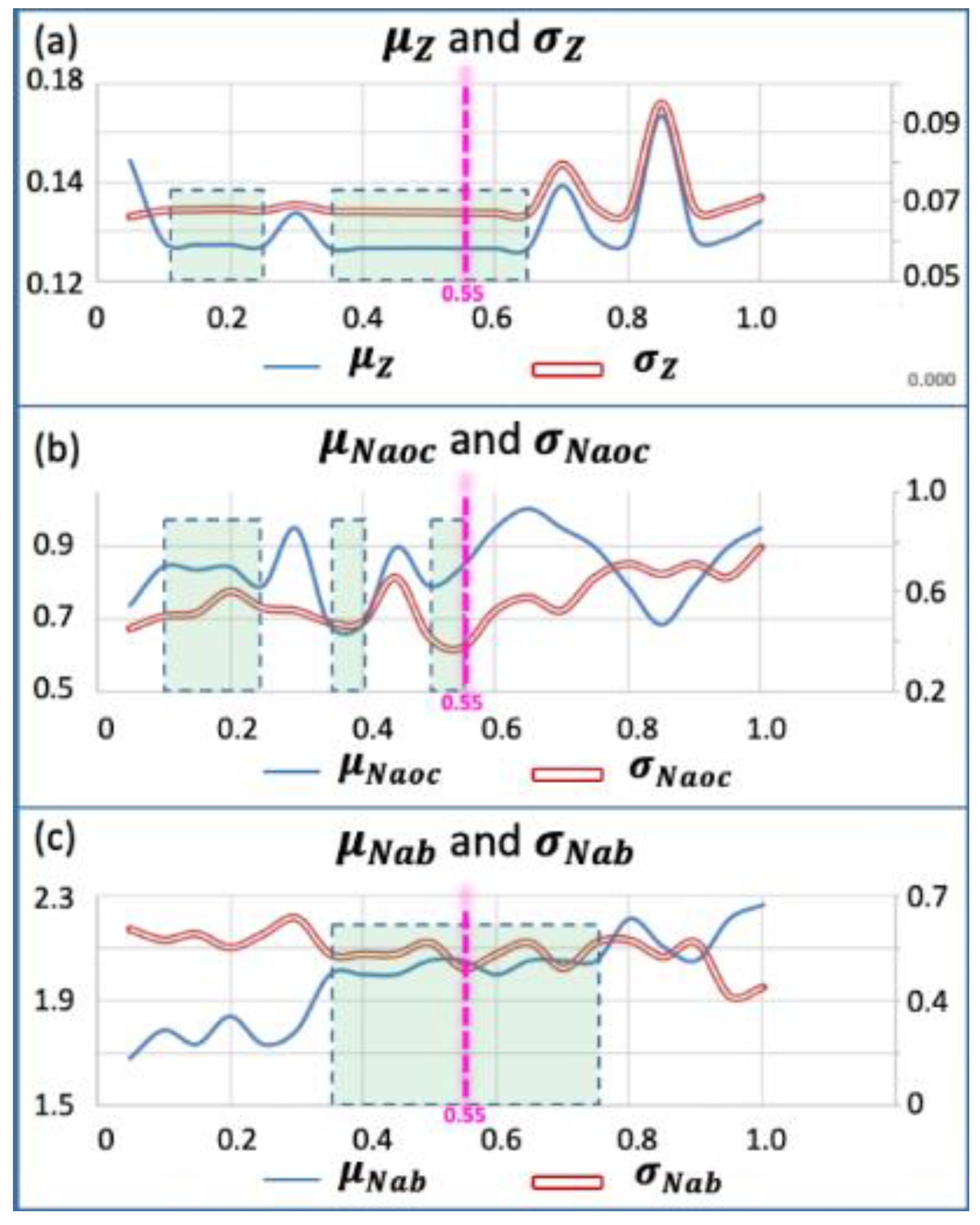
| DEI of μz | DEI of σz | DEI of μNaoc | DEI of σNaoc | DEI of μNab | DEI of σNab |
|---|---|---|---|---|---|
| [0, 0.1477] | [0, 0.0677] | [0, 0.82] | [0, 0.55] | [0, 1.95] | [0, 0.63] |
| Iteration | RMC | Weight-Sum Deviation | Number of Active Original Constraints | Number of Active Bounds | Better Than Cycle (t-1) | Better Than Best RMC | Update DEI | |||
|---|---|---|---|---|---|---|---|---|---|---|
| μz | σz | μNaoc | σNaoc | μNab | σNab | |||||
| 1 | 0.5 | 0.147 | 0.068 | 0.79 | 0.42 | 2.05 | 0.62 | - | - | [1, 1.95] -> [1, 2.05] |
| 2 | 1.0 | 0.152 | 0.071 | 0.95 | 0.78 | 2.26 | 0.45 | N | N | - |
| 3 | 0.8 | 0.148 | 0.068 | 0.79 | 0.71 | 2.21 | 0.63 | N | N | - |
| 4 | 0.6 | 0.147 | 0.067 | 0.95 | 0.52 | 2.00 | 0.58 | Y | Y | -> |
| 5 | 0.4 | 0.147 | 0.068 | 0.68 | 0.48 | 2.00 | 0.58 | Y | Y | - |
| 6 | 0.2 | 0.147 | 0.068 | 0.84 | 0.60 | 1.84 | 0.60 | N | N | -> |
| 7 | 0.3 | 0.154 | 0.069 | 0.95 | 0.52 | 1.79 | 0.71 | N | N | - |
| 8 | 0.45 | 0.147 | 0.068 | 0.89 | 0.66 | 2.00 | 0.58 | Y | N | - |
| 9 | 0.55 | 0.147 | 0.067 | 0.84 | 0.37 | 2.05 | 0.52 | Y | Y | - |
| 10 | 0.65 | 0.147 | 0.067 | 1.00 | 0.58 | 2.05 | 0.62 | N | N | -> |
| 11 | 0.48 | 0.147 | 0.068 | 0.89 | 0.66 | 2.05 | 0.62 | N | N | - |
| 12 | 0.53 | 0.147 | 0.067 | 0.84 | 0.69 | 2.00 | 0.58 | Y | N | - |
| 13 | 0.57 | 0.147 | 0.067 | 0.84 | 0.37 | 2.11 | 0.57 | N | N | - |
| 14 | 0.43 | 0.145 | 0.069 | 0.84 | 0.60 | 2.00 | 0.58 | N | N | - |
| ALPPL | ALP | ||
|---|---|---|---|
| General comparison | Search method | Rule-based parameter learning | Golden section search |
| Criteria used for evaluation of the RMC | Deviation (fulfillment of the goals), the robustness of the solution | Fulfillment of the goals | |
| If the approximation is sensitive to the scenario changing | Considering different scenarios, the most appropriate RMC is identified. The approximation is relatively insensitive to scenario changes | In each scenario, the best RMC is identified; it may vary as the scenario changes. The approximation is relatively sensitive to scenario changes | |
| Stopping criteria | The best RMC has not been updated for n iterations, or the total iteration number reaches a threshold | The distance between two golden section points is less than a threshold | |
| Complexity | O(n2) | O(n2) | |
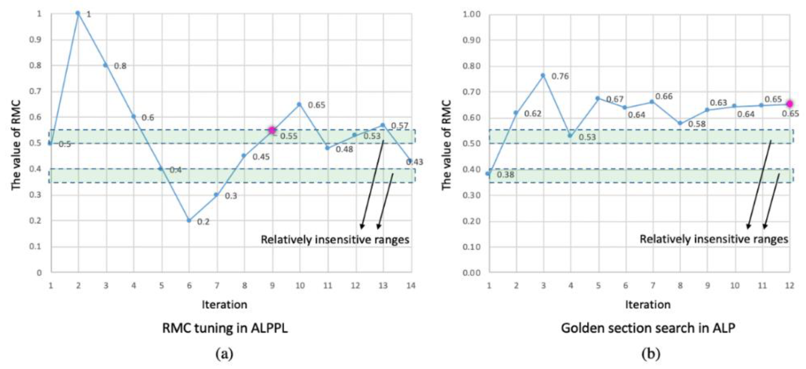
| Comparison of the cooling problem results | Number of search iterations | 14 | 12 |
| If the identified best RMC is in the insensitive range | Yes | No | |
| Number of tested RMC values falling into insensitive range | 4 | 2 | |
| Is the insensitive range explored sufficiently | Relatively sufficiently | Insufficiently |
Disclaimer/Publisher’s Note: The statements, opinions and data contained in all publications are solely those of the individual author(s) and contributor(s) and not of MDPI and/or the editor(s). MDPI and/or the editor(s) disclaim responsibility for any injury to people or property resulting from any ideas, methods, instructions or products referred to in the content. |
© 2024 by the authors. Licensee MDPI, Basel, Switzerland. This article is an open access article distributed under the terms and conditions of the Creative Commons Attribution (CC BY) license (https://creativecommons.org/licenses/by/4.0/).
Share and Cite
Guo, L.; Nellippallil, A.B.; Smith, W.F.; Allen, J.K.; Mistree, F. An Adaptive Linear Programming Algorithm with Parameter Learning. Algorithms 2024, 17, 88. https://doi.org/10.3390/a17020088
Guo L, Nellippallil AB, Smith WF, Allen JK, Mistree F. An Adaptive Linear Programming Algorithm with Parameter Learning. Algorithms. 2024; 17(2):88. https://doi.org/10.3390/a17020088
Chicago/Turabian StyleGuo, Lin, Anand Balu Nellippallil, Warren F. Smith, Janet K. Allen, and Farrokh Mistree. 2024. "An Adaptive Linear Programming Algorithm with Parameter Learning" Algorithms 17, no. 2: 88. https://doi.org/10.3390/a17020088
APA StyleGuo, L., Nellippallil, A. B., Smith, W. F., Allen, J. K., & Mistree, F. (2024). An Adaptive Linear Programming Algorithm with Parameter Learning. Algorithms, 17(2), 88. https://doi.org/10.3390/a17020088