

The Use of Correlation Features in the Problem of Speech Recognition


Abstract
:1. Introduction
2. Related Works and Presentation and Processing of Speech Messages
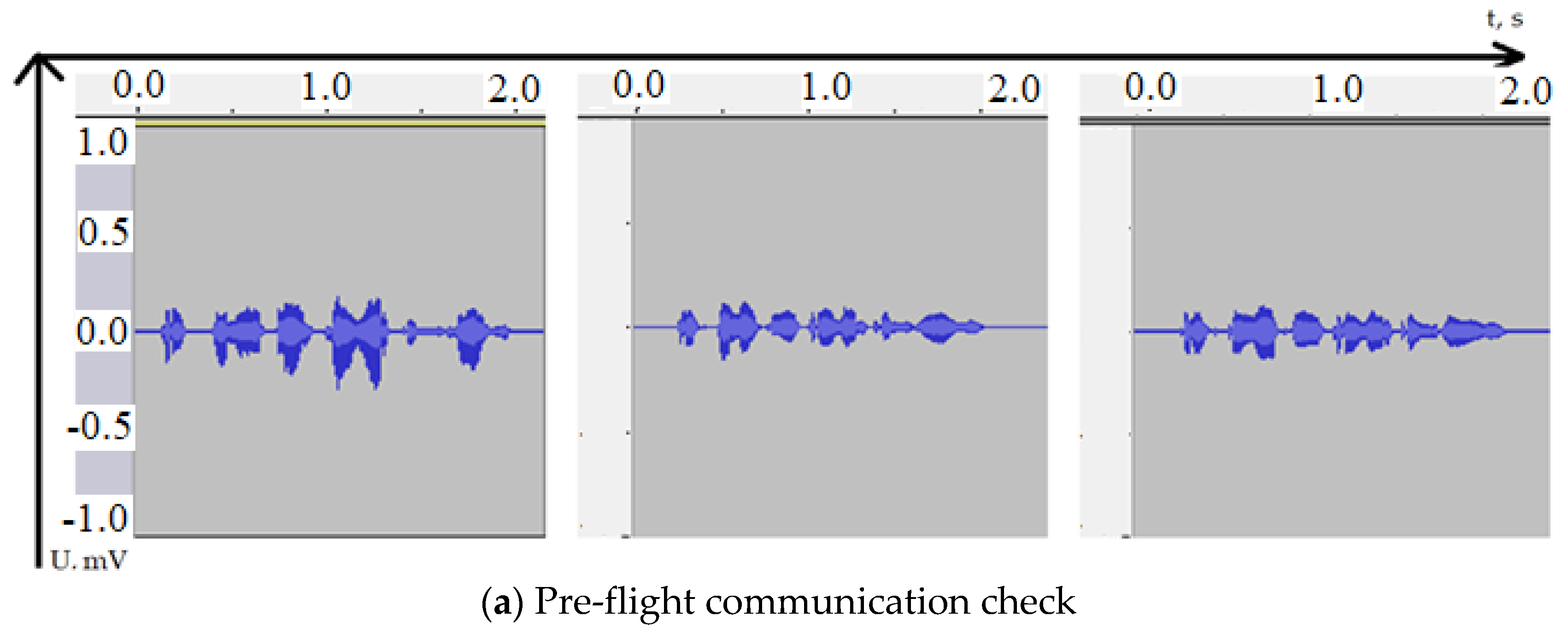
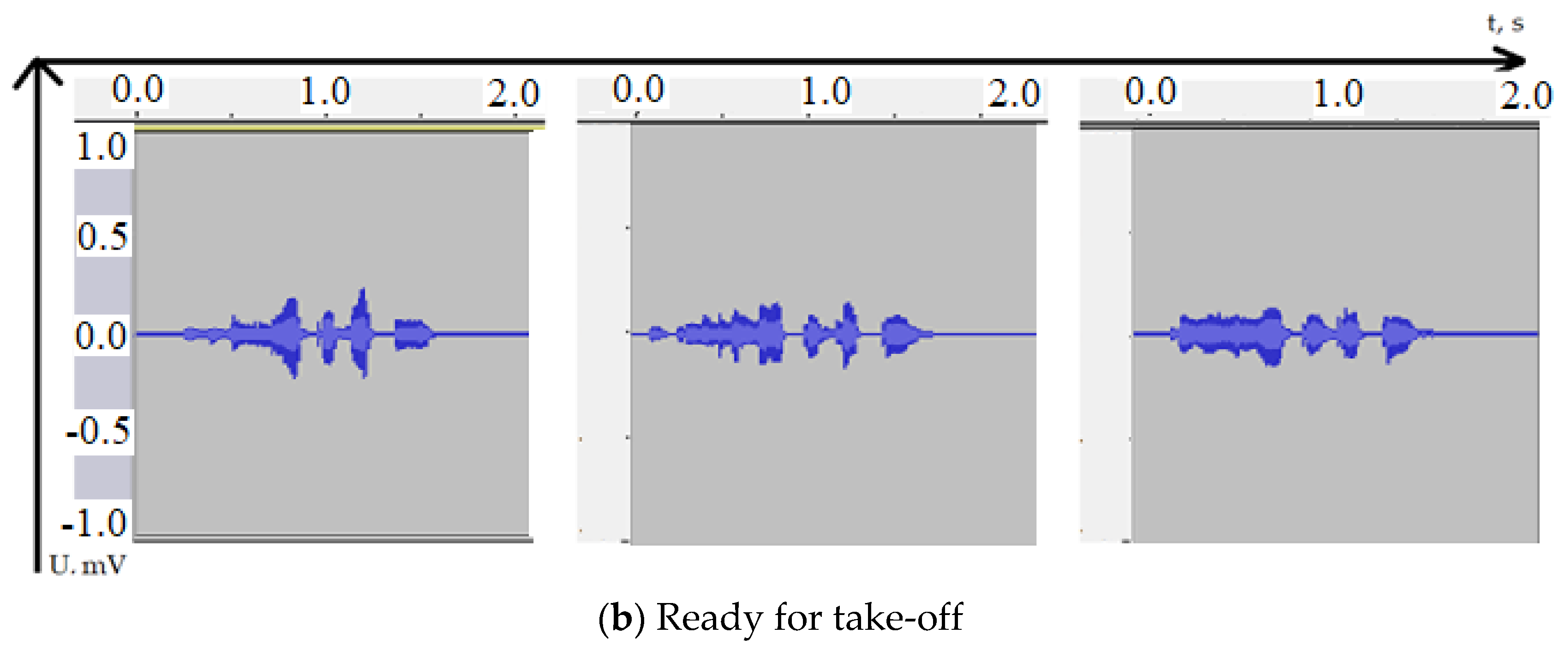
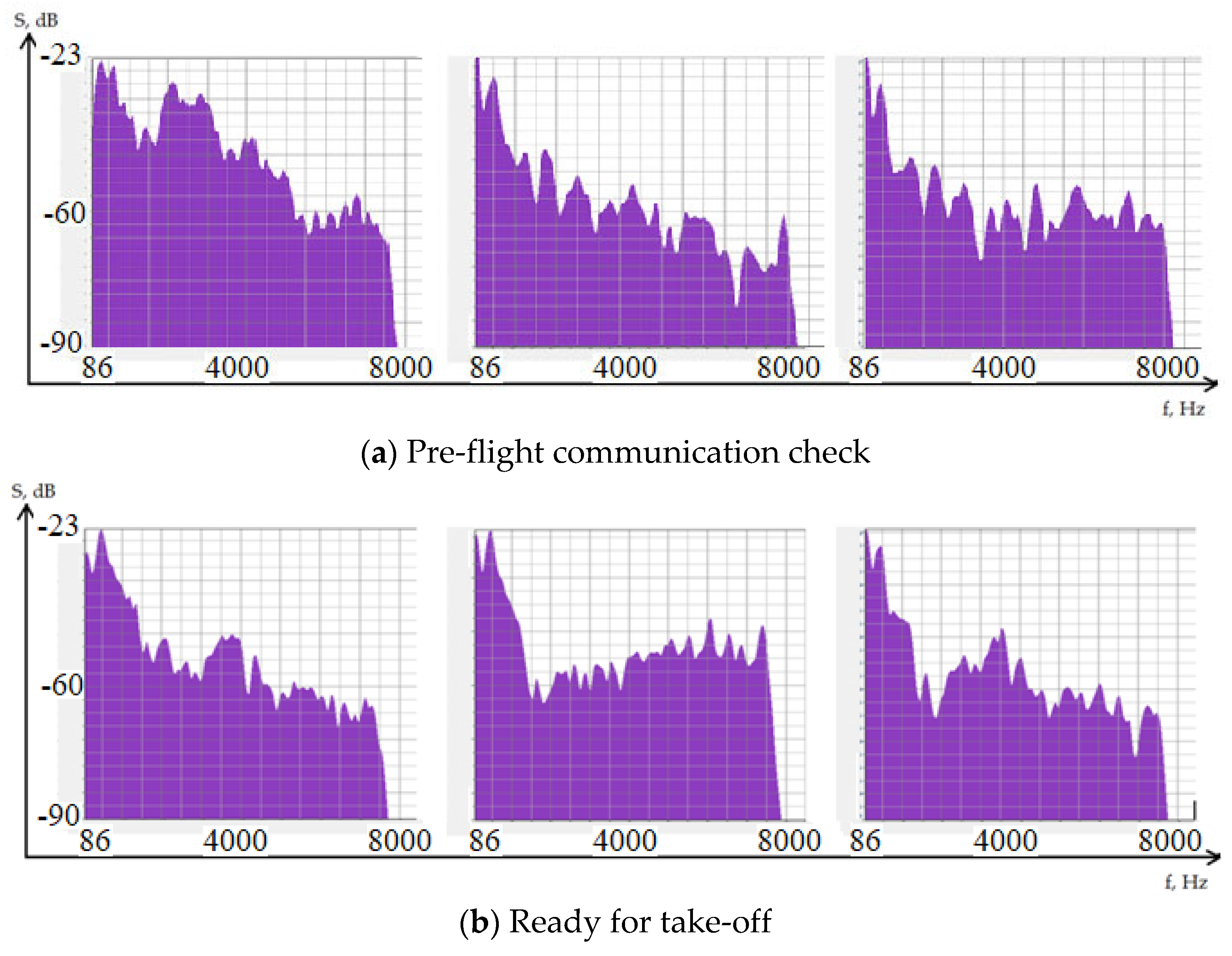
3. Materials and Methods
4. Results
5. Conclusions
Funding
Institutional Review Board Statement
Informed Consent Statement
Data Availability Statement
Conflicts of Interest
References
- Parekh, D.; Poddar, N.; Rajpurkar, A.; Chahal, M.; Kumar, N.; Joshi, G.P.; Cho, W. A Review on Autonomous Vehicles: Progress, Methods and Challenges. Electronics 2022, 11, 2162. [Google Scholar] [CrossRef]
- Khanum, A.; Lee, C.-Y.; Yang, C.-S. Deep-Learning-Based Network for Lane Following in Autonomous Vehicles. Electronics 2022, 11, 3084. [Google Scholar] [CrossRef]
- Brunelli, M.; Ditta, C.C.; Postorino, M.N. A Framework to Develop Urban Aerial Networks by Using a Digital Twin Approach. Drones 2022, 6, 387. [Google Scholar] [CrossRef]
- Andriyanov, N.; Vasiliev, K. Using Local Objects to Improve Estimation of Mobile Object Coordinates and Smoothing Trajectory of Movement by Autoregression with Multiple Roots. Adv. Intell. Syst. Comput. 2020, 1038, 1014–1025. [Google Scholar] [CrossRef]
- Jarray, R.; Bouallègue, S.; Rezk, H.; Al-Dhaifallah, M. Parallel Multiobjective Multiverse Optimizer for Path Planning of Unmanned Aerial Vehicles in a Dynamic Environment with Moving Obstacles. Drones 2022, 6, 385. [Google Scholar] [CrossRef]
- Andriyanov, N.A. Combining Text and Image Analysis Methods for Solving Multimodal Classification Problems. Pattern Recognit. Image Anal. 2022, 32, 489–494. [Google Scholar] [CrossRef]
- Mukhamadiyev, A.; Khujayarov, I.; Djuraev, O.; Cho, J. Automatic Speech Recognition Method Based on Deep Learning Approaches for Uzbek Language. Sensors 2022, 22, 3683. [Google Scholar] [CrossRef]
- Ramos-Pérez, E.; Alonso-González, P.J.; Núñez-Velázquez, J.J. Multi-Transformer: A New Neural Network-Based Architecture for Forecasting S & P Volatility. Mathematics 2021, 9, 1794. [Google Scholar] [CrossRef]
- Andriyanov, N.; Papakostas, G. Optimization and Benchmarking of Convolutional Networks with Quantization and OpenVINO in Baggage Image Recognition. In Proceedings of the 2022 VIII International Conference on Information Technology and Nanotechnology (ITNT), Samara, Russia, 23–27 May 2022; pp. 1–4. [Google Scholar] [CrossRef]
- Wu, X.; Jin, Y.; Wang, J.; Qian, Q.; Guo, Y. MKD: Mixup-Based Knowledge Distillation for Mandarin End-to-End Speech Recognition. Algorithms 2022, 15, 160. [Google Scholar] [CrossRef]
- Andriyanov, N.; Dementiev, V.; Gladkikh, A. Analysis of the Pattern Recognition Efficiency on Non-Optical Images. In Proceedings of the 2021 Ural Symposium on Biomedical Engineering, Radioelectronics and Information Technology (USBEREIT), Yekaterinburg, Russia, 13–14 May 2021; pp. 0319–0323. [Google Scholar] [CrossRef]
- Rizà Porta, R.; Sterchi, Y.; Schwaninger, A. How Realistic Is Threat Image Projection for X-ray Baggage Screening? Sensors 2022, 22, 2220. [Google Scholar] [CrossRef]
- Ribas, D.; Miguel, A.; Ortega, A.; Lleida, E. Wiener Filter and Deep Neural Networks: A Well-Balanced Pair for Speech Enhancement. Appl. Sci. 2022, 12, 9000. [Google Scholar] [CrossRef]
- Antonetti, A.E.d.S.; Siqueira, L.T.D.; Gobbo, M.P.d.A.; Brasolotto, A.G.; Silverio, K.C.A. Relationship of Cepstral Peak Prominence-Smoothed and Long-Term Average Spectrum with Auditory–Perceptual Analysis. Appl. Sci. 2020, 10, 8598. [Google Scholar] [CrossRef]
- Andriyanov, N.; Andriyanov, D. Intelligent Processing of Voice Messages in Civil Aviation: Message Recognition and the Emotional State of the Speaker Analysis. In Proceedings of the 2021 International Siberian Conference on Control and Communications (SIBCON), Kazan, Russia, 13–15 May 2021; pp. 1–5. [Google Scholar] [CrossRef]
- Andriyanov, N.A. Recognition of radio exchange voice messages in aviation based on correlation analysis. Izv. Samara Sci. Cent. Russ. Acad. Sci. 2021, 23, 91–96. [Google Scholar] [CrossRef]
- LeCun, Y.; Bengio, Y.; Hinton, G. Deep learning. Nature 2015, 521, 436–444. [Google Scholar] [CrossRef]
- Dhouib, A.; Othman, A.; El Ghoul, O.; Khribi, M.K.; Al Sinani, A. Arabic Automatic Speech Recognition: A Systematic Literature Review. Appl. Sci. 2022, 12, 8898. [Google Scholar] [CrossRef]
- Nallasamy, U.; Metze, F.; Schultz, T. Active Learning for Accent Adaptation in Automatic Speech Recognition. In Proceedings of the 2012 IEEE Spoken Language Technology Workshop (SLT), Miami, FL, USA, 2–5 December 2012; pp. 360–365. [Google Scholar]
- Wahyuni, E.S. Arabic Speech Recognition Using MFCC Feature Extraction and ANN Classification. In Proceedings of the 2017 2nd International Conferences on Information Technology, Information Systems and Electrical Engineering (ICITISEE), Yogyakarta, Indonesia, 1–2 November 2017; pp. 22–25. [Google Scholar]
- Trinh Van, L.; Dao Thi Le, T.; Le Xuan, T.; Castelli, E. Emotional Speech Recognition Using Deep Neural Networks. Sensors 2022, 22, 1414. [Google Scholar] [CrossRef]
- Satt, A.; Rozenberg, S.; Hoory, R. Efficient Emotion Recognition from Speech Using Deep Learning on Spectrograms. In Proceedings of the International Speech Communication Association (INTERSPEECH), Stockholm, Sweden, 20–24 August 2017; pp. 1089–1093. [Google Scholar]
- Aksyonov, K.; Antipin, D.; Afanaseva, T.; Kalinin, I.; Evdokimov, I.; Shevchuk, A.; Karavaev, A.; Chiryshev, U.; Talancev, E. Testing of the Speech Recognition Systems Using Russian Language Models. CEUR Workshop Proc. 2018, 2298, 1–7. [Google Scholar]
- Vazhenina, D.; Kipyatkova, I.; Markov, K.; Karpov, A. State-of-the-art speech recognition technologies for Russian language. HCCE’12. In Proceedings of the 2012 Joint International Conference on Human-Centered Computer Environments, Aizu-Wakamatsu, Japan, 8–13 March 2012; pp. 59–63. [Google Scholar] [CrossRef]
- Bagley, S.; Antonov, A.; Meshkov, B.; Sukhanov, A. Statistical Distribution of Words in a Russian Text Collection. In Proceedings of the Dialogue 2009, Bekasovo, Serbia, 27–31 May 2009; pp. 13–18. [Google Scholar]
- Alqadasi, A.M.A.; Sunar, M.S.; Turaev, S.; Abdulghafor, R.; Hj Salam, M.S.; Alashbi, A.A.S.; Salem, A.A.; Ali, M.A.H. Rule-Based Embedded HMMs Phoneme Classification to Improve Qur’anic Recitation Recognition. Electronics 2023, 12, 176. [Google Scholar] [CrossRef]
- Oh, D.; Park, J.-S.; Kim, J.-H.; Jang, G.-J. Hierarchical Phoneme Classification for Improved Speech Recognition. Appl. Sci. 2021, 11, 428. [Google Scholar] [CrossRef]
- Liu, Z.; Huang, Z.; Wang, L.; Zhang, P. A Pronunciation Prior Assisted Vowel Reduction Detection Framework with Multi-Stream Attention Method. Appl. Sci. 2021, 11, 8321. [Google Scholar] [CrossRef]
- Jeon, S.; Kim, M.S. Noise-Robust Multimodal Audio-Visual Speech Recognition System for Speech-Based Interaction Applications. Sensors 2022, 22, 7738. [Google Scholar] [CrossRef] [PubMed]
- Vazhenina, D.; Markov, K. End-to-End Noisy Speech Recognition Using Fourier and Hilbert Spectrum Features. Electronics 2020, 9, 1157. [Google Scholar] [CrossRef]
- Pervaiz, A.; Hussain, F.; Israr, H.; Tahir, M.A.; Raja, F.R.; Baloch, N.K.; Ishmanov, F.; Zikria, Y.B. Incorporating Noise Robustness in Speech Command Recognition by Noise Augmentation of Training Data. Sensors 2020, 20, 2326. [Google Scholar] [CrossRef] [PubMed]
- Andriyanov, N.A.; Andriyanov, D.A. The using of data augmentation in machine learning in image processing tasks in the face of data scarcity. J. Phys. Conf. Ser. 2020, 1661, 012018. [Google Scholar] [CrossRef]
- Box, G.; Jenkins, G.; Reinsel, G. Time Series Analysis; John Wiley & Sons, Inc.: Hoboken, NJ, USA, 2008; p. 755. [Google Scholar]
- Draper, N.R.; Smith, H. Applied Regression Analysis; Wiley: New York, NY, USA, 1966; p. 407. [Google Scholar]
- Zhihua, W.; Yongbo, Z.; Huimin, F. Autoregressive Prediction with Rolling Mechanism for Time Series Forecasting with Small Sample Size. Math. Probl. Eng. 2014, 2014, 572173. [Google Scholar]
- Orzechowski, A.; Bombol, M. Energy Security, Sustainable Development and the Green Bond Market. Energies 2022, 15, 6218. [Google Scholar] [CrossRef]
- Prajakta, S.K. Time series Forecasting using Holt-Winters Exponential Smoothing. Kanwal Rekhi Sch. Inf. Technol. J. 2004, 13, 1–13. [Google Scholar]
- Suyamto, D.; Prasetyo, L.; Setiawan, Y.; Wijaya, A.; Kustiyo, K.; Kartika, T.; Effendi, H.; Permatasari, P. Measuring Similarity of Deforestation Patterns in Time and Space across Differences in Resolution. Geomatics 2021, 1, 464–495. [Google Scholar] [CrossRef]
- Zulifqar, A. Forecasting Drought Using Multilayer Perceptron Artificial Neural Network Model. Adv. Meteorol. 2017, 2017, 5681308. [Google Scholar]
- Sherstinsky, A. Fundamentals of Recurrent Neural Network (RNN) and Long Short-Term Memory (LSTM) Network. Phys. D Nonlinear Phenom. 2020, 404, 132306. [Google Scholar] [CrossRef]
- Andriyanov, N.A.; Dementiev, V.E.; Tashlinskii, A.G. Detection of objects in the images: From likelihood relationships towards scalable and efficient neural networks. Comput. Opt. 2022, 46, 139–159. [Google Scholar] [CrossRef]
- Dua, S.; Kumar, S.S.; Albagory, Y.; Ramalingam, R.; Dumka, A.; Singh, R.; Rashid, M.; Gehlot, A.; Alshamrani, S.S.; AlGhamdi, A.S. Developing a Speech Recognition System for Recognizing Tonal Speech Signals Using a Convolutional Neural Network. Appl. Sci. 2022, 12, 6223. [Google Scholar] [CrossRef]
- Salas-Páez, C.; Quintana-Romero, L.; Mendoza-González, M.A.; Álvarez-García, J. Analysis of Job Transitions in Mexico with Markov Chains in Discrete Time. Mathematics 2022, 10, 1693. [Google Scholar] [CrossRef]
- Yohannes, Y.; Webb, P. Classification and Regression Trees, CART: A User Manual for Identifying Indicators of Vulnerability to Famine and Chronic Food Insecurity; International Food Policy Research Institute: Washington, DC, USA, 1999; p. 59. [Google Scholar]
- Pehlivanoglu, I.V.; Atik, I. Time series forecasting via genetic algorithm for turkish air transport market. J. Aeronaut. Space Technol. 2016, 9, 23–33. [Google Scholar]
- Wenzel, F.; Galy-Fajou, T.; Deutsch, M.; Kloft, M. Bayesian Nonlinear Support Vector Machines for Big Data. In Machine Learning and Knowledge Discovery in Databases: European Conference, ECML PKDD 2017, Skopje, Macedonia, 18–22 September 2017, Proceedings, Part I; Springer: Cham, Switzerland, 2017; pp. 307–322. [Google Scholar]
- Kozionova, A.P.; Pyaita, A.L.; Mokhova, I.I.; Ivanov, Y.P. Algorithm based on the transfer function model and one-class classification for detecting the anomalous state of dams. Inf. Control. Syst. 2015, 6, 10–18. [Google Scholar]
- Timina, I.; Egov, E.; Yarushkina, N.; Kiselev, S. Identification anomalies the time series of metrics of project based on entropy measures. Interact. Syst. Probl. Hum. Comput. Interact. 2017, 1, 246–254. [Google Scholar]
- Woods, J.W.; Dravida, S.; Mediavilla, R. Image Estimation Using Doubly Stochastic Gaussian Random Field Models. Pattern Anal. Mach. Intell. 1987, 9, 245–253. [Google Scholar] [CrossRef]
- Danilov, A.N.; Andriyanov, N.A.; Azanov, P.T. Ensuring the effectiveness of the taxi order service by mathematical modeling and machine learning. J. Phys. Conf. Ser. 2018, 1096, 012188. [Google Scholar] [CrossRef]
- Andriyanov, N.; Dementiev, V.; Tashlinskiy, A. Development and Research of Intellectual Algorithms in Taxi Service Data Processing Based on Machine Learning and Modified K-means Method. In Intelligent Decision Technologies. Smart Innovation, Systems and Technologies; Springer: Singapore, 2022; Volume 309, pp. 183–192. [Google Scholar] [CrossRef]
- Armer, A.I. Modeling and Recognition of Speech Signals Against the Background of Intense Interference. Ph.D. Thesis, Ulyanovsk State Technical University, Ulyanovsk, Russia, 20 June 2006; pp. 1–190. [Google Scholar]
- Krasheninnikov, V.R.; Lebedeva, E.Y.; Kapyrin, V.K. Variation of the boundaries of speech commands to improve the recognition of speech commands by their cross-correlation portraits. In Proceedings of the Samara Scientific Center of the Russian Academy of Sciences, Samara, Russia, 20–21 November 2013; Volume 15, pp. 928–930. [Google Scholar]
- Ayvaz, U.; Guruler, H.; Khan, F.; Ahmed, N.; Whangbo, T.; Abdusalomov, A. Automatic Speaker Recognition Using Mel-Frequency Cepstral Coefficients Through Machine Learning. Comput. Mater. Contin. 2022, 71, 5511–5521. [Google Scholar] [CrossRef]
- Khan, F.; Tarimer, I.; Alwageed, H.S.; Karadağ, B.C.; Fayaz, M.; Abdusalomov, A.B.; Cho, Y.-I. Effect of Feature Selection on the Accuracy of Music Popularity Classification Using Machine Learning Algorithms. Electronics 2022, 11, 3518. [Google Scholar] [CrossRef]
- Audacity. Available online: https://www.audacityteam.org/ (accessed on 11 January 2023).

| Algorithm | Pros | Cons |
|---|---|---|
| Regression models | Simplicity, high level of knowledge | Narrow scope, strong retrainability, the need for combined time series |
| Autoregressive models | Taking into account the internal connections of the signal, the developed mathematical apparatus | Impossibility of describing signals with a complex structure |
| Exponential smoothing models | Smoothing out slowly changing signals in noisy environments | Inability to describe speech signals with high accuracy |
| Models on the most similar pattern | Adequate description of normal data | Impossible to represent heterogeneous data |
| Artificial neural networks | Flexible parameter setting, high accuracy | High computational costs, high model complexity, low stability |
| Markov chains | Simplicity, taking into account the dynamics of random processes | Too short memory for describing speech signals |
| Classification-regression trees | Good interpretability of results, sufficiently high accuracy | Strong retrainability of models |
| Genetic algorithm | Wide application, relatively high efficiency | High computational cost |
| Support vector machine | Working with non-linear connections, flexible settings | Necessity of preprocessing, searching for parameters |
| Transfer function | Adequate description of complex data | High computational cost, low performance |
| Fuzzy logic | Universality of approach, probabilistic estimates | Inability to accurately describe speech messages, complexity of mathematical analysis |
| Doubly stochastic models | Ability to describe inhomogeneous and non-stationary signals | Difficulty in identifying model parameters |
| Algorithm | Accuracy |
|---|---|
| Decision tree (depth 10) | 92.50% |
| Support vector machine | 93.50% |
| Fully connected neural network (3 layers, 20-20-20 neurons) | 94.25% |
| Recurrent neural network (recurrent layer 24 neurons) | 95.50% |
| Long Short Term Memory Network (LSTM layer 24 neurons) | 96.00% |
| 1D Convolutional Neural Network (16 filters) | 94.00% |
| Fully Connected Network based on correlation function | 96.50% |
| Recurrent network based on correlation function | 97.25% |
| LSTM network based on correlation function | 97.50% |
| Convolutional network based on correlation function | 95.75% |
| Convolutional network based on correlation portrait | 97.50% |
| Algorithm | Processing Time, ms |
|---|---|
| Decision tree (depth 10) | 2.35 |
| Support vector machine | 8.94 |
| Fully connected neural network (3 layers, 20-20-20 neurons) | 246.80 |
| Recurrent neural network (recurrent layer 24 neurons) | 320.55 |
| Long Short Term Memory Network (LSTM layer 24 neurons) | 654.35 |
| 1D Convolutional Neural Network (16 filters) | 806.20 |
| Fully Connected network based on correlation function | 246.80 + 18.40 |
| Recurrent network based on correlation function | 320.55 + 18.40 |
| LSTM network based on correlation function | 654.35 + 18.40 |
| Convolutional network based on correlation function | 806.20 + 18.40 |
| Convolutional network based on correlation portrait | 2325.62 |
| Algorithm | q = 0.1 | q = 1 | q = 10 |
|---|---|---|---|
| Decision tree (depth 10) | 35.75% | 78.25% | 92.50% |
| Support vector machine | 37.00% | 75.50% | 93.25% |
| Fully connected neural network (3 layers, 20-20-20 neurons) | 45.75% | 87.25% | 94.25% |
| Recurrent neural network (recurrent layer 24 neurons) | 54.25% | 83.75% | 95.50% |
| Long short term memory network (LSTM layer 24 neurons) | 49.75% | 80.50% | 96.00% |
| 1D convolutional neural network (16 filters) | 39.50% | 86.25% | 94.00% |
| Fully connected network based on correlation function | 57.25% | 92.25% | 96.50% |
| Recurrent network based on correlation function | 59.00% | 93.25% | 97.25% |
| LSTM network based on correlation function | 52.25% | 94.00% | 97.50% |
| Convolutional network based on correlation function | 51.00% | 91.00% | 95.75% |
| Convolutional network based on correlation portrait | 53.25% | 96.75% | 97.50% |
Disclaimer/Publisher’s Note: The statements, opinions and data contained in all publications are solely those of the individual author(s) and contributor(s) and not of MDPI and/or the editor(s). MDPI and/or the editor(s) disclaim responsibility for any injury to people or property resulting from any ideas, methods, instructions or products referred to in the content. |
© 2023 by the author. Licensee MDPI, Basel, Switzerland. This article is an open access article distributed under the terms and conditions of the Creative Commons Attribution (CC BY) license (https://creativecommons.org/licenses/by/4.0/).
Share and Cite
Andriyanov, N. The Use of Correlation Features in the Problem of Speech Recognition. Algorithms 2023, 16, 90. https://doi.org/10.3390/a16020090
Andriyanov N. The Use of Correlation Features in the Problem of Speech Recognition. Algorithms. 2023; 16(2):90. https://doi.org/10.3390/a16020090
Chicago/Turabian StyleAndriyanov, Nikita. 2023. "The Use of Correlation Features in the Problem of Speech Recognition" Algorithms 16, no. 2: 90. https://doi.org/10.3390/a16020090
APA StyleAndriyanov, N. (2023). The Use of Correlation Features in the Problem of Speech Recognition. Algorithms, 16(2), 90. https://doi.org/10.3390/a16020090