Abstract
This paper investigates the systematic and complete usage of k-opt permutations with in application to local optimization of symmetric two-dimensional instances up to points. The proposed method utilizes several techniques for accelerating the processing, such that good tours can be achieved in limited time: candidates selection based on Delaunay triangulation, precomputation of a sparse distance matrix, two-level data structure, and parallel processing based on multithreading. The proposed approach finds good tours (excess of 0.72–8.68% over best-known tour) in a single run within 30 min for instances with more than points and specifically 3.37% for the largest examined tour containing points. The new method proves to be competitive with a state-of-the-art approach based on the Lin–Kernigham–Helsgaun method (LKH) when applied to clustered instances.
1. Introduction
The history of the travelling salesman problem (TSP) dates back to a book published in 1832 which mentioned optimal routes for the first time [1]. The first person who formulated this as a mathematical optimization problem was probably Karl Menger [2]. At a mathematical colloquium in Vienna in 1930, he talked about “the task of finding the shortest path connecting the points for a finite number of points whose pairwise distances are known.” This problem can be stated with following cost function to be minimized:
where the selection of points is decided based on a permutation vector of length N according to . The cost function is the sum of all Euclidean distances between pairs of neighbouring points.
A tour is usually modelled as a graph with nodes from the set V (a.k.a. vertices) and edges from set E, where the nodes correspond to points and the edges connect the points in pairs. The distance between two points corresponds to the length of the connecting edge.
This optimization problem continues to attract many researchers to this day. Originally treated as a two-dimensional problem with symmetric distances as described above, several variants of the original problem have been formulated and studied up to the present.
The methods to deal with the TSP can be divided into exact solvers, which provide the global optimum (i.e., the shortest possible tour), and heuristics trying to find a solution which is at least close to the optimum. The time needed to find the exact solution grows exponentially with the number of tour points (see, for instance, [3]). Implementations for exact solvers are freely available for academic use [4] (www.math.uwaterloo.ca/tsp/concorde/ (accessed on 7 December 2022)). Hougardy and Zhong have created special instances that are difficult to solve with exact solvers [5].
In contrast, suboptimal solutions can be found in reasonable time by suitable heuristics. A state-of-the-art heuristic has been developed by Helsgaun [6] (http://webhotel4.ruc.dk/~keld/research/LKH-3/LKH-3.0.7.tgz (accessed on 7 December 2022)). Equipped with various of tour-improvement tools, it has even been able to find optimal tours for instances up to 85 900 points.
Christofides and Serdyukov independently proposed an algorithm that guarantees solutions within a factor of 1.5 of the optimal tour length (excess ≤ 50%) if the instance is symmetric and obeys the triangle inequality [7,8]. In [9], it was theoretically proven that a ()-approximation can be obtained in -time. This work was extended by [10].
The most successful heuristics are based on the chained Lin–Kernigham method [11], which is one of the methods that try to optimize the entire tour by local improvements. It relies on the ideas of [12,13] and applies sequences of typically only 2-opt and 3-opt permutations. A k-opt permutation intersects a tour of connected points at k locations, i.e., k edges are removed from the graph and k other edges are inserted, ideally shorter on average than the original edges. A tour is called k-optimal if no further improvements can be obtained by using m-opt permutations with . There are also studies including 4-opt and 5-opt [14]. Such k-opt permutations steer the solution to a minimum, which is typically not the global one. Laporte gave a concise tour of the subject in [15].
In addition to the classical TSP, optimization problems with special constraints have also been studied, such as the vehicle-routing problem, in which not only the distances between points count, but also time constraints and multiple agents with varying capacities have to be considered [16,17]. A comprehensive overview is given in [18]. Time-dependent TSPs were investigated by [19,20], wherein the costs depend not only on the distances between points but are also a function of the position within the tour.
A generalized TSP was presented in [21], wherein points are clustered and the tour to be optimized consist of exactly one point of each cluster. This problem was addressed with a genetic algorithm. Several applications of clustered TSPs were discussed in [22]. Time constraints have also been an issue recently in solving TSPs with constraint programming [23]. The authors of [24] proposed a technique allowing permutations that do not directly lead to a shorter tour and thus can avoid getting stuck in local minima. It can compete with the Lin–Kernigham–Helsgaun (LKH, [6]) method for difficult problems when starting from a random tour i.e., without creating an initial tour.
As already pointed out above, the local optimisation by k-opt permutations and similar operations runs the risk of getting stuck in a local minimum. There are different strategies to overcome this problem. In [25], for example, a “breakout local search” was proposed to jump from one local minimum to the next and hopefully better local minimum, which of course requires several attempts. A very successful recombination technique initially generates many suboptimal tours converging at different local minima (see for example [26,27]). In [26], this is described as “principle of backbone edges”. These are connections between points that are present in all quickly solved tours. The entire tour can then be collapsed into a smaller tour that considers only the remaining missing connections, whereas a path of backbone edges is taken into account as a single edge. A comparison of techniques can be found in [28] and the literature cited therein. These ideas of combining information from different trials are closely related to so-called “ant colony optimization” methods whereby the decision-making mimics the use of pheromone trails of ants. Recent developments and relevant citations can be found in [29].
However, such recombination techniques and other metaheuristics are not practical for very large instances with more than one million points, because even finding the first local minimum can be very time consuming.
Many proposed heuristics only deal with small or medium-sized instances [30,31,32,33,34,35,36,37,38], whereas in [39] problems with even billions of cities are tackled. In the last decade, heuristics based on the idea of swarm intelligence like ant colonization and others have been become quite popular [29,32,33,35,37,38,40]. However, so far they cannot really compete with state-of-the-art methods like LKH when applied to classical TSP problems.
The processing of large instances can be accelerated by decomposing the tour into shorter subtours which remain connected by using fixed edges [41,42]. This could be combined by using multiple threads and parallel processing on multicore processors [29,42] or by taking advantage of graphical processing units [43].
The method described in this paper draws on many ideas proposed by various researchers and combines them with new ideas. It aims at optimizing very large instances (up to 10 million points, symmetric Euclidean two-dimensional distances) in a single pass in limited time. To achieve this goal, various techniques are implemented to speed up the processing. The vast number of possible permutations is reduced by a suitable candidate selection based on Delaunay triangulation [44]. This also allows the precomputation of a sparse distance matrix. As an alternative to the use of a single-level permutation vector, a two-level data structure is considered, and parallel processing based on multithreading is supported. The main contribution of the proposed method is to provide and investigate an alternative to chained Lin–Kernigham method by systematically applying k-opt permutations with . Therefore, the proposed method does not consider recombination or other metaheuristics to escape from local minima, but concentrates on the acceleration of the first run. A dedicated software has been written from scratch. For initial tour generation, candidate set enrichment is proposed and the use of a cluster-based technique [42] is considered. The developed code will be made available as open source to allow reproducible research on this topic.
2. Methods
2.1. Basics of k-Opt Permutations
Suppose a tour consists of ten points numbered from zero to nine. Their current order can be represented by a permutation vector
The order of points is cyclic, that is, points 0 and 9 are direct neighbours and the order of points could be alternatively represented as follows:
A so-called k-opt operations changes the order of points such that the sequence of points is cut at k positions. For example, a 2-opt operation might cut the entire sequence between points 2 and 3 and between 6 and 7:
The only operation (or permutation) that can now be performed is an inversion of the cut section leading to [45]. In terms of tour length, this is equivalent to turning the outer segment around: . The higher k is chosen, the more different permutations can be performed. For example, for there are five new possibilities:
For many k-opt permutations, the same result can be achieved by a subsequent application of permutations with fewer cuts. For example, permutation 3 from the above list of 3-opt permutations could be performed by two 2-opt permutations:
In theory, to find a permutation that can shorten the tour, all points must be considered as intersection positions. The complexity of a pure 2-opt approach would be and grows to about for 3-opt permutations. It becomes obvious that such an approach becomes infeasible for higher values of k when focusing on large instances with N > 10,000.
2.2. Candidates Selection
As pointed out in the previous subsection, an increasing number of cuts (increasing k for k-opt) leads to exponential explosion of possible permutations making this approach too time-consuming. An intelligent approach would ignore those permutations which are most unlikely to lead to an improvement. It should consider only permutations which connect points that are close to each other. In other words, a set of good candidates has to be determined for each point.
Helsgaun had proposed a so-called -measure which evaluates the cost increase when a minimum 1-tree is required to contain the edge [46,47]. The five -nearest points proved to be an excellent set of candidates. Johnson [48] suggested using the least costly edges in each of the four geometric quadrants (for 2-dimensional instances) around a point, which may also be helpful for clustered instances in addition to the -measure [6].
The proposed method does not maintain any trees such a minimum 1-tree or similar; instead it uses Delaunay triangulation to find suitable candidates. This approach had been proposed by Reinelt for the first time [49] and was also recently adopted in [50]. It has the advantage that neighbours in all directions are automatically considered, even though one or more close neighbours might be missed. We apply the Fortune’s sweepline algorithm described in [51] by adapting the software written and provided by Fortune himself. Delaunay triangulation leads to an average of six candidates per point, Table 1.

Table 1.
Number of candidates per point determined via Delaunay triangulation.
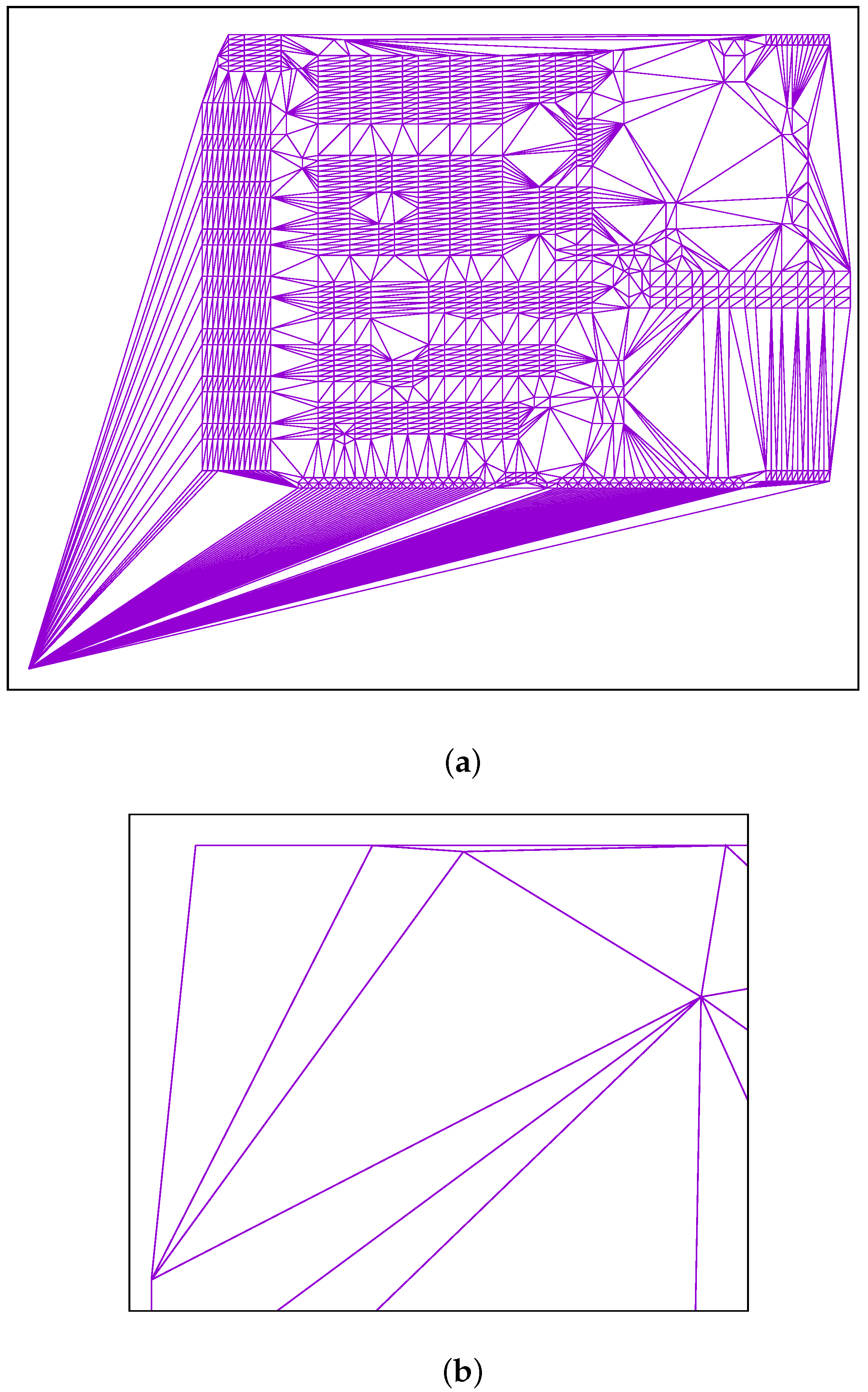
However, extremal points that are far from all other points can have many more candidates assigned to them as can be seen for d1291 and lra498378. Figure 1 shows two special cases of many and few candidates per point.
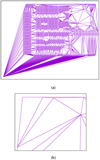
Figure 1.
Triangulation of point clouds: (a) d1291 showing a high number of candidates for the bottom left point; (b) close-up of pr2392 showing the top left point with only two edges, i.e., two candidates.
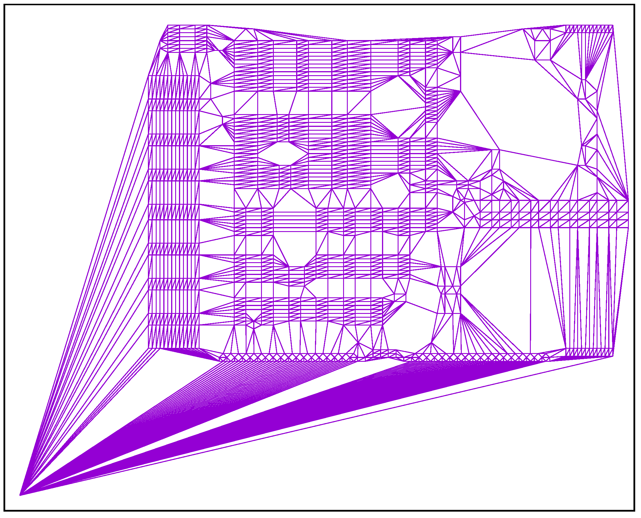
The use of candidate sets can greatly reduce the number of permutations to be examined per point, but it is also likely that the procedure will miss good neighbours and, accordingly, will not find some connections (edges) that belong to the optimal tour. The implemented software allows us to determine the maximum number of allowed candidates per point to be used. Then only the closest neighbours are taken into account. When the set of candidates is limited to , for example, then some edges remain unconsidered as can be seen in Figure 2 in comparison to Figure 1a. Interestingly, the point at the bottom left is still connected to many other points. This is just because the point is itself one of the five Delaunay candidates for these other points.

Figure 2.
Resulting mesh when considering only the five closest candidates per point for TSP instance d1291.
As the points and their assigned candidate neighbours are frequently inspected during the optimization process, the corresponding distances between them are precomputed, leading to a very sparse distance matrix that can be stored efficiently.
2.3. Initial Tour Generation
The local optimization methods discussed in this paper are less effective and time-consuming when applied to an arbitrary (or even random) order of points. The importance of appropriate initial-tour generation has already been pointed out in [52]. The proposed method employs two different techniques, which are briefly discussed in the following subsections.
2.3.1. Greedy Tour Based on Candidates Paths (GrebCap)
The first implemented method belongs to the group of greedy tour generators. It starts at an arbitrary point. Its candidate set is examined, and the closest candidate is chosen as the next point. After inserting a point into the tour, it is marked to avoid multiple consideration. This continues, always taking the closest available candidate. When the procedure reaches a point whose candidates have all already been integrated into the tour, the path is saved and any available point is taken as the starting point of the next path.
This procedure results in a certain number of paths which have to be connected to form a complete tour. Starting from an endpoint of any first path, a nearest-neighbour approach looks for an end point of another path which has the shortest distance. Both paths are linked to form a joint path. This is repeated until all paths constitute a Hamiltonian circle.
The nearest neighbour method has a complexity of . Obviously, building the paths accelerates the whole process of finding near neighbours, because the number of path endpoints is much lower than the total number of tour points. It has been observed that the average path length depends on the chance that a path can be extended by a free point from the candidates set. On average, such a set consists of six adjacent points as shown in Table 1. However, if one increases the number of candidates, the average path length becomes longer, the number of paths decreases, and the number N of points to be compared for nearest neighbour search also decreases, speeding up the tour-generation process.
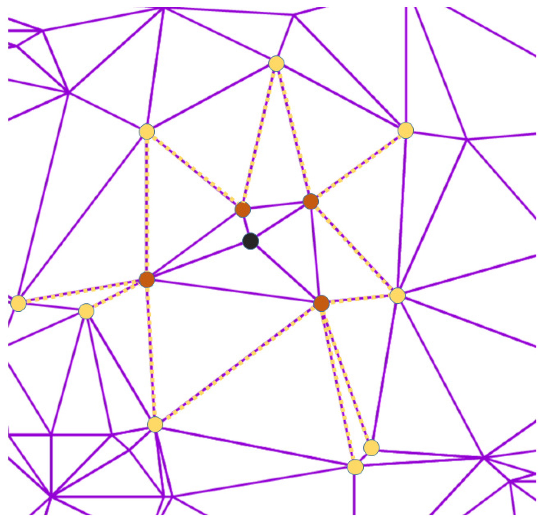
Therefore, an enrichment of the candidates sets is proposed, which considers not only the neighbours from the Delaunay triangulation but additionally the neighbours of all Delaunay candidates. This is illustrated for a particular point in Figure 3. After triangulation, only four neighbouring points (in brown) are candidates of the black point in the centre of the figure. This set is extended by also including the candidates (shown in yellow) of the brown points, so that in total of 13 candidates are available. This augmentation of the Delaunay set also had been mentioned in [49].

Figure 3.
Candidates set for a point (black) from TSP instance gil262. The original set after Delaunay triangulation is shown in brown, and the enriched set additionally contains the points marked with yellow colour.
If the black point in Figure 3 were the endpoint of a constructed intermediate path when taking only the original candidates set into account, then the additional candidates drastically increase the chance that the path can be continued in the near vicinity without a time-consuming search for the nearest neighbour. This candidate enrichment increases the number of candidates per point from an average of six to approximately 20.
The creation of paths as described above sometimes results in very short segments. For these snippets, it is beneficial to individually insert their points into existing paths. The selection of suitable insertion positions is achieved based on the closest candidates of the point to be inserted. Based on systematic tests, it has been found that the integration of snippets with a maximum of 25 points not only fasten the entire procedure but additionally shorten the length of the initial tour.
Table 2 contains the results of initial tour generation with GrebCap for different TSP instances with increasing number of points.

Table 2.
Quality of initial tours dependent on chosen method (excess over best known tour) and duration for building the tour. The number of points per instance is given in the file names.
Because the initial tour varies slightly depending on the chosen starting point when connecting points to paths, the program was executed 10 times for each instance and the average was taken as the result.
The excess is computed as
It is mostly between 20% and 30% if the points are more or less randomly distributed. For clustered datasets, the excess even rises to over 45% for santa1437195. For Tnm100000, the excess is rather small because the points are arranged along six straight lines, which also facilitates the greedy initial tour generation. It can also be seen that the time to generate the initial tour is negligible for small instances and increases rapidly for tours containing more than 0.5 million points. The enrichment of the candidate sets together with the merging of snippet points into close paths significantly reduces the complexity to a tolerable amount of time even for the largest instance E10M.0 (column “enriched + merged”). Additionally, it can also be observed that the tour lengths get distinctly shorter (lower excess). This improved initial tour generation is called GrebCap+ in the following.
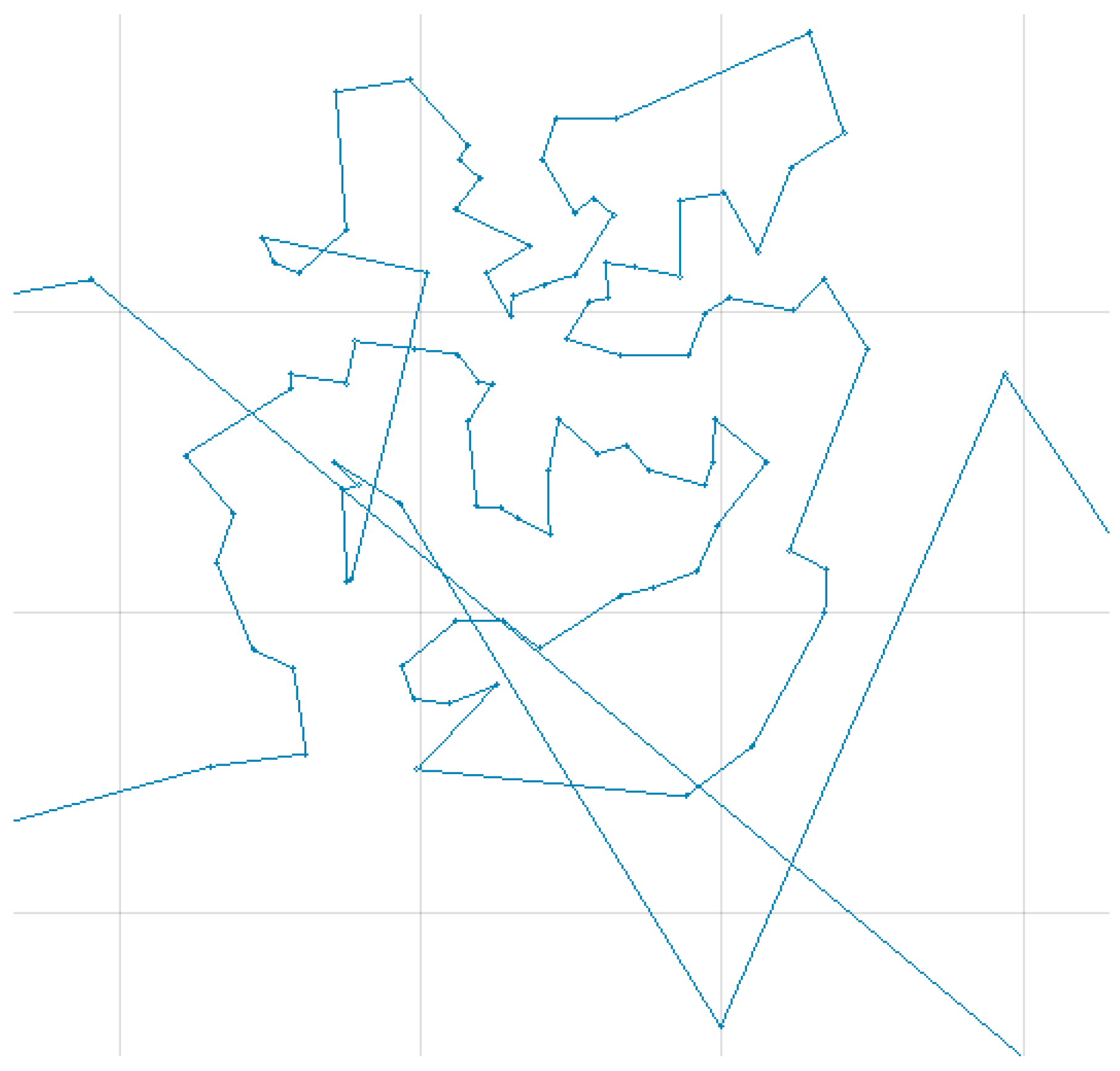
This improved greedy tour generation is a straightforward procedure, works quite well, and is also reasonably fast for the largest instance. However, despite methodological improvements, it cannot prevent the use of long edges across the point region, resulting in tours with relatively high excesses compared to the best-known tours. In Figure 4, it can be seen that points, which had not been considered in the greedy path extension, are finally connected via rather long edges in the search for the nearest neighbour.
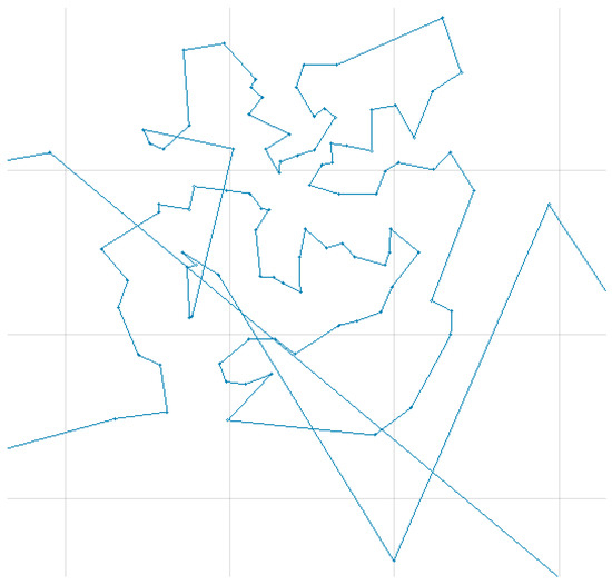
Figure 4.
Magnified region of the initial tour based on GrebCap+ for C100k.0 showing the initial tour with unfavourable long edges.
2.3.2. Double Local Optimization with Recursion (DoLoWire)
In [42], a more sophisticated approach called “double local optimization with recursion” had been proposed which reduces the algorithmic complexity via clustering of points. Based on these clusters, first a coarse tour is generated that connects the cluster centroids. This coarse tour contains about 1500 points at default settings and defines the order of the clusters. In case a cluster contains too many points with respect to a threshold, the procedure is applied recursively. A nearest neighbour approach searches for the shortest connections between points of adjacent clusters. All points within a cluster form a subtour with fixed endpoints and these subtours are optimized by using a brute-force 3-opt optimizer with a maximum of five loops over all points. There is no random component involved, i.e., each execution results in the same tour. The rightmost columns of Table 2 contain the corresponding results.
As the execution times for small instances suggest, the clustering of DoLoWire is somewhat more complex than the GrebCap initialization. Processing times again increase with the number of points. However, this relation is not monotonic because the processing depends on how the clusters fit the distribution of points. Most importantly, DoLoWire yields much better tours, which reduces the time for subsequent local optimization based on k-opt operations.
2.4. Local Optimization Using k-Opt Permutations
Based on the introduction of k-opt permutations in Section 2.1, it will now be explained how candidates can be efficiently used for search-space reduction when looking for shorter tours.
2.4.1. Optimization with 2-Opt Permutations
If we consider only 2-opt permutation, two cut positions must be defined in the entire sequence of points. Let us call the point to the left of the first cut P. If there are N points in the tour, we have to access N different positions of P when looking for permutations that shorten the tour. Theoretically, the second cut position could also be anywhere on the tour. However, if we know the possible candidates – let us call them Pc – this variety reduces to the number of candidates. The underlying assumption is that a permutation shortens the length of the tour if it makes P and Pc direct neighbours in the tour. Table 3 shows the two possible 2-opt permutations that have the potential to achieve the goal.

Table 3.
List of possible 2-opt operations based on a 7-points example.
The vertical separator lines indicate the locations where the original sequence of points was separated.
Reversing the point sequence between the two intersections (i.e., performing a flip operation) brings the point P and its candidate together. Clearly, these 2-opt permutations need not be tested if P and Pc are already adjacent neighbours in the tour.
If the cut position is set to the right of the point P, then the second cut position is also to the right of the candidate point Pc. Alternatively, both intersections are performed to the left of points P and Pc leading to another modification of the point sequence. These two permutations are not redundant because 0 and 4 are not necessarily neighbours in the Delaunay graph.
The terms “right neighbour” and “left neighbour” are synonyms for successor and predecessor, respectively. The focus on specific points reveals that the proposed approach is point-centric while approaches based on a graph model typically are edge-centric.
2.4.2. Optimization with 3-Opt Permutations
Although the selection and application of 2-opt permutations are fairly straightforward, the selection of 3-opt permutations needs more thought. As the tour is now cut at three locations, two additional points, Q and its candidates Qc, can be used to define the objective of a permutation.
Because the tour is cut to the right of P, its current neighbour should also find a new matching partner from its candidates set. For this reason, the current right neighbour of P is called Q:
This assignment has the great advantage of avoiding a second loop over all tour points, which reduces the complexity of searching for improving permutations.
Table 4 shows the two variants how the candidates Pc and Qc can be located and it lists in part (a) the possible permutations that match the pairs (P,Pc) and (Q,Qc) when the cyclic order of the four points is PQ→Pc→Qc.

Table 4.
List of possible 3-opt operations based on a 10-points example: (a) circular order PQ→Pc→Qc; (b) circular order PQ→Qc→Pc.
The 10-point examples assign P, Q, Pc, and Qc to the points 1, 2, 5, and 8. After performing a permutation, points 1 and 5 as well as 2 and 8 have become neighbours.
In the case in which Qc lies between Q and Pc with respect to the current cyclic order of points, a single 3-opt permutation can be applied (Table 4b). All permutations have in common that the removal of three edges creates six points that have to be reconnected to each other. For only four of them (P, Q, Pc, Qc), the new neighbour is preselected, whereas the remaining two points automatically become new neighbours. This ensures a certain degree of freedom in the sense that even those points can become neighbours that are not candidates of each other.
The pseudocode of the optimization process is given in Listing 1.
| Listing 1. Pseudocode of 2+3-opt optimizer. See text for details. |
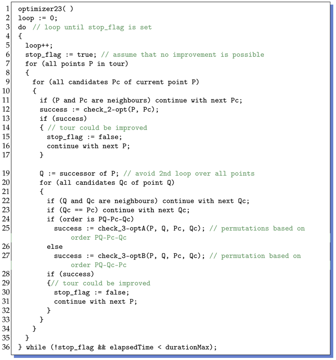 |
In total, three loops are required: one over all points in the tour specifying point P and two more (much shorter) loops over all candidates Pc and Qc. When looking for a suitable point Qc, it does not need to be checked against P because P is a neighbour of Q and the check in line 21 already verifies that Q and Qc are not neighbours. Once an improving permutation could be found, it is applied to the tour and the next point P is examined. This process continues until either no more improving permutations could be found or a maximum duration is reached.
2.4.3. Optimization with 5-Opt Permutations
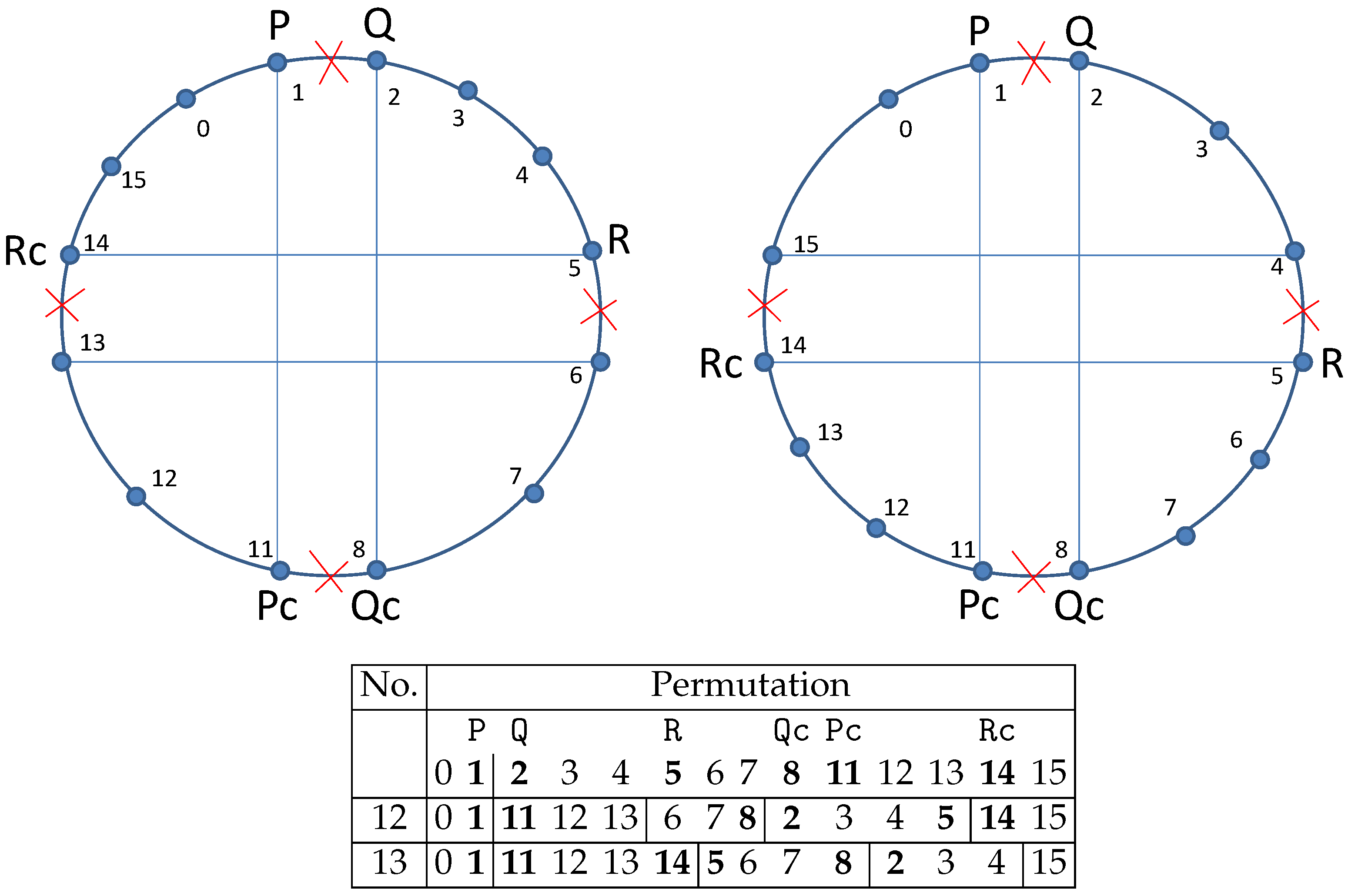
Following the logic of connecting points with one of their candidates, 4-opt permutations are not feasible when a new pair of points (R, Rc) is introduced. For this reason, 5-opt permutations are discussed in this subsection. Later it will turn out that these automatically include 4-opt permutations.
With respect to the initial cyclic order of P, Pc, Q, Qc, R, and Rc, there are 12 variants. Each order allows a specific number of different permutations (see Table 5).

Table 5.
Possible cyclic orders of points in 5-opt operations and number of different possible permutations.
Finding all possible permutations (172 in total) is a combinatorial problem. It has been solved by using a dedicated software that applies a systematic search and ignores such permutations that could be achieved by simpler operations. Note that the points P,Q,R are defined to be in cyclic order of
and each of them always appears before its corresponding candidate Pc,Qc,Rc:
The anchor of this cyclic ordering is set at point P.
Table 6 contains the four reasonable permutations for case PQ→Qc→R→Rc→Pc.

Table 6.
Possible 5-opt operations based on a 16-points example if the circular order is PQ→Qc→R→Rc→Pc: (a) all 16 points exist; (b) points 9 and 10 do not exist.
The removal of five edges demands the reconnection of ten points, from which three pairings (P|Pc,Q|Qc,R|Rc = ) are enforced by selecting candidates.
Examining the permutation 7, we can deduce the following. If R and Rc were already direct neighbours (i.e., the points 9 and 10 do not exist), then the application of 7 would be a sole 3-opt operation, which additionally would become the same permutation as 8 (see Table 6b). Numbers 9 and 10 would collapse to 4-opt permutations. However, the proposed algorithm ignores configurations where a point and its candidate are already direct neighbours. A practical example can be given if the order of points is PQ→Qc→R→Pc→Rc, Table 7.

Table 7.
Example of a 5-opt operations that can collapse to 4-opt operation: (a) all 16 points exist; (b) points 9 and 10 do not exist.
Again, we explore the case in which points 9 and 10 are not present, which means R and Pc are direct neighbours. The 5-opt permutation now collapses to a 4-opt operation. There are many other arrangements where this can happen. In other words, 4-opt operations are already contained in the proposed 5-opt mechanism.
In many publications a special 4-opt permutation called “double-bridge move” is discussed. Figure 5 shows two variants of it with respect to the implemented permutations.
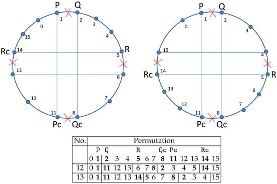
Figure 5.
Special 4-opt permutation in two variants: “double-bridge move”.
In both cases, the points Pc and Qc have to be direct neighbours in the tour, i.e., the points 9 and 10 do not exist.
2.4.4. Optimization with 6-Opt Permutations
One innovation of the proposed method is to include 6-opt operations. Consistent with the explanations in the previous subsections, a fourth point pair (S, Sc) is introduced. Identical to the assignment of P and Q as being direct neighbours, now S is defined as successor of R:
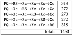
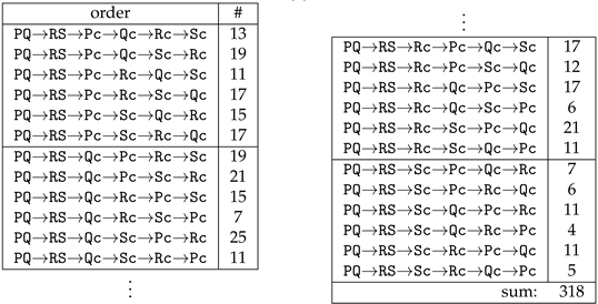
There are five possibilities (0…4) of how many candidates are between the pairs PQ and RS. Table 8a shows these possibilities and also contains the number of different permutations that could be performed for a given order of points.

Table 8.
Possible orders of points in 6-opt operations and number of different possible permutations: (a) general overview; (b) specific cases of PQ→RS→Xc→Xc→Xc→Xc.
The case PQ→RS→Xc→Xc→Xc→Xc is given in detail for all possible successions of candidates (Table 8b). A total of 1450 different 6-opt permutations can be identified. A dedicated software has been written that has determined all of these variants and has output pieces of source code which are integrated in the TSP software, allowing the systematic check of all permutations. Note that the candidates Rc and Sc only have to obey
The proposed method systematically investigates and applies 2-opt to 6-opt operation and is therefore called Sys2to6 hereafter. The corresponding complete algorithm is presented in Listing 2. It is basically an extension of Listing 1 and additionally comprises three nested loops: one over the selection of point R and two further over the candidates Rc and Sc. Theoretically, R could be taken at any position in the tour except for positions that are already occupied by P, Pc, Q and Qc. This would drive the complexity beyond . Practically, the selection of R starts as a successor of Q and can be bounded by a certain edge distance maxEdgeDist from Q without compromising the effectiveness of the optimization process too much. Corresponding results will be presented in Section 3.
| Listing 2. Pseudocode of Sys2to6 optimizer. See text for details |
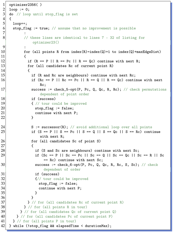 |
From the pseudocode and the data on the different k-opt operations, it can be deduced that 2-opt permutations can be performed the fastest, whereas as k increases, more and more time is needed to check all the different positions and variants of permutations. In general, it is important that the for-loop over points P is executed as often as possible. For this reason, the implemented schedule (varying from Listing 2) is as follows. In the first loop, only check_2-opt() is called. Starting with the second loop also check_3-opt() is invoked. It is monitored how many permutations could be successfully performed within a whole loop over P. If this number falls below an empirical threshold of , k is increased from either 3 to 5 or from 5 to 6. This threshold provides a good compromise between staying in fast mode with asymptotic convergence toward a local k-opt minimum and switching to a slower mode with prospects of going beyond this minimum.
2.5. Parallel Processing
Despite the algorithmic enhancements introduced, the time-complexity can still be too high for very large TSP instances. To achieve the goal of creating a good tour in limited time (30 min for example), parallel processing has to be considered. The challenging task is to split the processing into jobs which do not interfere with each other. Generally, the success of each permutation to be tested depends on all preceding permutations, because it is a sequential process. The most promising method for parallelization is to divide the initial suboptimal tour into two or more consecutive nonoverlapping segments and treat each segment as a separate tour. However, these subtours may not be optimized as closed-loop tours, but as open-loop tours because the connections between the subsequent segments must be preserved.
2.5.1. Open-Loop Optimization of Subtours
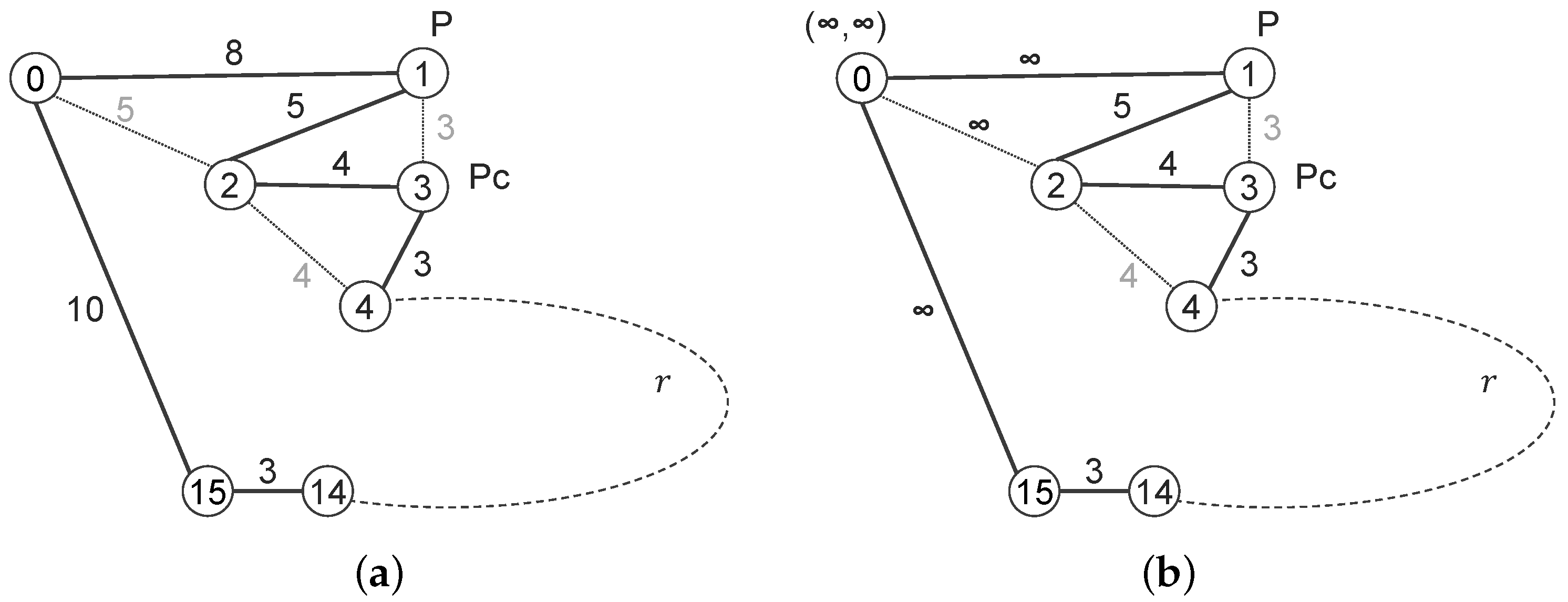
Fränti et al. proposed the use of pseudonodes to achieve open-loop optimization without changing the underlying closed-loop optimization method [53]. However, the problem at hand not only requires an open loop but also the endpoints, where the loop is open, are known and must persist as endpoints of the segment. To satisfy this condition, the author proposes to complement the set of points with a virtual point that is connected to both endpoints and is positioned at . Let us take a look at the example tour in Figure 6a.
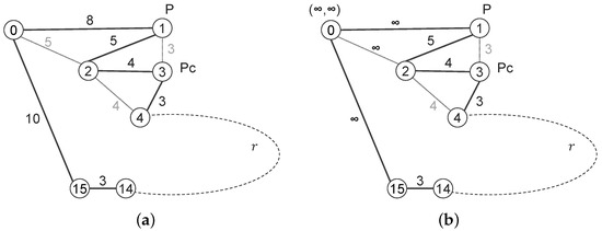
Figure 6.
Example with virtual point explaining subtour optimization: (a) closed-loop tour; (b) open-loop subtour with virtual point at infinite location. Black, grey, and dashed lines show current edges, possible edges after permutation, and arbitrary sequence of points, respectively. See text for further details.
It consists of an arbitrary large set of points, from which seven points are drawn. The edges are annotated with the distances between the points and the total tour length is currently . Using a 2-opt permutation which arranges P and Pc as direct neighbours, the order of points can be changed to and the tour length decreases to . Assuming that the points 1 and 15 are the endpoints of a subtour, the permutation discussed would be forbidden, because point 1 is now hidden between points 2 and 3.
In Figure 6b, the point 0 is considered a virtual point augmenting the subtour from point 1 to point 15. The location of this virtual point is purposively defined as . The distances to all other points automatically become infinite. The discussed permutation is no longer possible because it would substitute two edges (0–1 and 2–3) of common length by two new edges (0–2 and 1–3) with a joint length of . Both lengths are infinite and this permutation is not considered as an improvement. In other words, the edges between the virtual point and the two endpoints remain untouched. After the subtour is optimized, the virtual point is removed and the endpoints can be reconnected with the endpoints of the adjacent subtours.
Nevertheless, it is still possible to make P and Pc neighbours by replacing edges (1–2 and 3–4) with common length by two new edges (1–3 and 2–4) with a joint length of . The new order would be .
2.5.2. Multithreading
Having discussed how to handle subtours without changing their endpoints, now their integration into the global optimization will be described.
The complete algorithm is shown in Listing 3. Depending on the number of jobs to be executed in parallel, the number of points per segment is derived from the total number N of points. The last segment is slightly shorter if (line 20). All segments are independently optimized by using a virtual point as described above (lines 16–38). After execution, the modified order of points has to be mapped back to the global permutation vector (line 39).
| Listing 3. Pseudo code multi-threading. See text for details. |
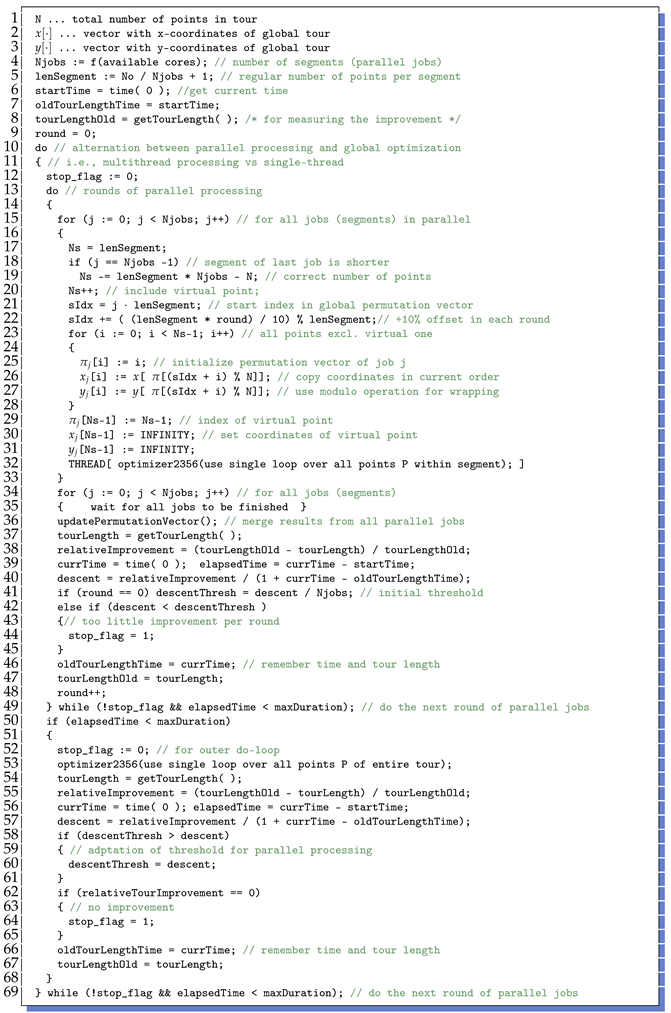 |
Obviously, for each subtour, separate candidate sets have to be determined, which do not contain any relations between subtours. This represents some computational overhead. The establishment of edges between different subtours is only possible if the segmentation of the entire tour is varied. For this reason, the segment borders are shifted by 10% of the segment length in each round (line 23). As this exchange between subtours is essential for finding best neighbours for all points, the subtours are not fully optimized but a single loop is performed over all points P.
In the first round, all jobs commonly start with 2-opt operations only. After a round is completed, a check is made to see if the next k-opt mode has been activated in at least one of the jobs. If so, this mode is also enabled for all other jobs in next round. The main reason for using a common mode is to maximize the utilization of all CPU cores, which is achieved when all jobs take approximately the same time.
As an example, consider a vector of 10 points, the current order of which is given by . This could be the order of points after the initial tour generation. Suppose there are two jobs to be processed in parallel, both starting with a sorted order of points and augmentation with an additional virtual point: . After separate optimization, the order of points in the first segment could be and in the second . Note that the virtual points still lie between points 4 and 0. The underlying optimization algorithm further ensures that point 0 remains in first place. The new order of points can be mapped back by using the algorithm depicted in Listing 4. It explains how the segment-wise permutation is applied to the global permutation vector. The main step is performed in line 19. Here, the global permutation vector is accessed via a start index and the permutation vector of a particular segment s. The start index points at the position from which the segment points were initially taken, specifies the order in which the elements have to be read. Because the order of the elements is circular, the modulo operations with the total number of points wraps the access to the start of . The temporary vector now contains the new order of the points and this information has to be copied back into (line 23). With respect to the example, the temporary vector is equal to for the first segment and equal to for the second. The new global permutation vector is then .
| Listing 4. Pseudocode showing how individual segment permutations are mapped back to the global permutation vector. See text for details |
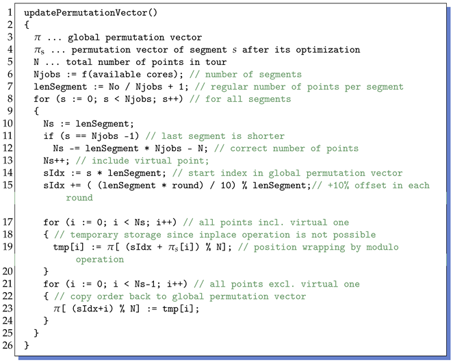 |
It has to be mentioned that the optimization of segments could also lead to instead of . The circular arrangement is the same but the direction is reversed and the virtual point is now not located at the end of the vector but at second position. Therefore, values (including the virtual point) are copied to the temporary vectors. The correct mapping to can easily be caught up by exception handling.
The given example is summarized in Figure 7.

Figure 7.
Example of mapping optimization information from two segments back to global permutation vector . The virtual points V in correspond to the index 5 in this example. See text for further details.
It can be seen that the endpoints of the segments and remain neighbours.
2.5.3. Scheduling for Fastest Descent
It has already been mentioned above that the exchange of information between segments is made possible by shifting the segment borders in each round of parallel processing. However, this exchange can only occur between adjacent segments. In the case of clustered instances in particular, this procedure may miss some important permutations, which can only be found when processing the entire tour. For this reason, a special scheduling is implemented that alternates between parallel processing and global optimization.
The alteration is triggered by a descent measure (Listing 3, lines 8, 9, 41–51; 58–65)
trying to find the fastest path to the optimal tour. After the first round (using only 2-opt) has been performed, a descent threshold is initialized based on the current descent measure (line 41). The idea is to perform fast parallel processing as long as possible before starting potentially more time-consuming global processing. As soon as the descent falls below this threshold after a certain round of parallel processing, the inner do-loop is exited and a single-threaded job is used to optimize the entire tour (line 53). If the resulting descent is lower than the current threshold, the threshold is updated accordingly (lines 58–61). The outer do-loop (lines 10, 69) involves the interleaving of multithread and single-thread processing.
2.6. Data Structure
The classical and clearest data structure for maintaining the order of points is based on a permutation vector as already used above. This vector contains indices pointing at the point coordinates in their current order.
There is one drawback in using such a permutation vector. All indices that are involved in a permutation have to be accessed and moved to their new positions. The time to flip a segment, for example, is proportional to the length of this segment which can be in worst case. This can be avoided by using hierarchical structures. A comprehensive comparison of different data structures which can be used in the context of TSP has been given in [54]. Among other things, the authors have discussed a two-level data structure, in which the point level is supplemented by a parent level that virtually splits the whole tour into segments.
At this parent level, the order of parent nodes defines the order of segments at point level. The number of parent nodes (and thus the number of segments) is set to about leading to segments with an average length of approximately . For detailed explanations, the reader is referred to [54]. The benefit lies in the fact that it is not necessary to access every single point (or its index) involved in a permutation operation, but the points can be processed in chunks. This means that mostly the parent nodes have to be reordered and the point segments only come into play for the chunks where the permutation cuts are located. Flipping operations can be signalled by a flag indicating that all points of a chunk are in reverse order. The complexity decreases from to . The factor expressed the computational overhead of maintaining the two-level structure, which can be enormous. As soon as a chunk needs to be split, because the permutation cut is located somewhere between its points, some of the points must be moved to a neighbouring chunk, changing the chunk length . A special mechanism keeps track of these lengths ensuring .
The advantage of the two-level structure becomes noticeable only when N is large enough. The implemented structure is even more complicated than described in [54] because the indices of all points must also be derivable with respect to the entire tour. By using these indices, the circular order of the points and their candidates must be determined as described in Section 2.4.2.
3. Investigations
3.1. Data and Hardware
The implementation of the proposed method has been tested on several TSP instances chosen from different repositories. The focus was on very large instances and instances with varying characteristics. The compiled set of instances can be found at [55]. All research reported here has been performed on a Linux server equipped with an AMD EPYC 7452 CPU (2.35 GHz, 32 cores, 128 MB) and 125.7 GiB RAM. The source code (ANSI-C) utilizes the Linux-specific pthread library for parallel processing and has been compiled with gcc and option ‘-Ofast’. Alternatively, the code can be compiled on computers running Windows operation systems. However the source code does not support parallel processing under Windows yet.
3.2. General Behaviour
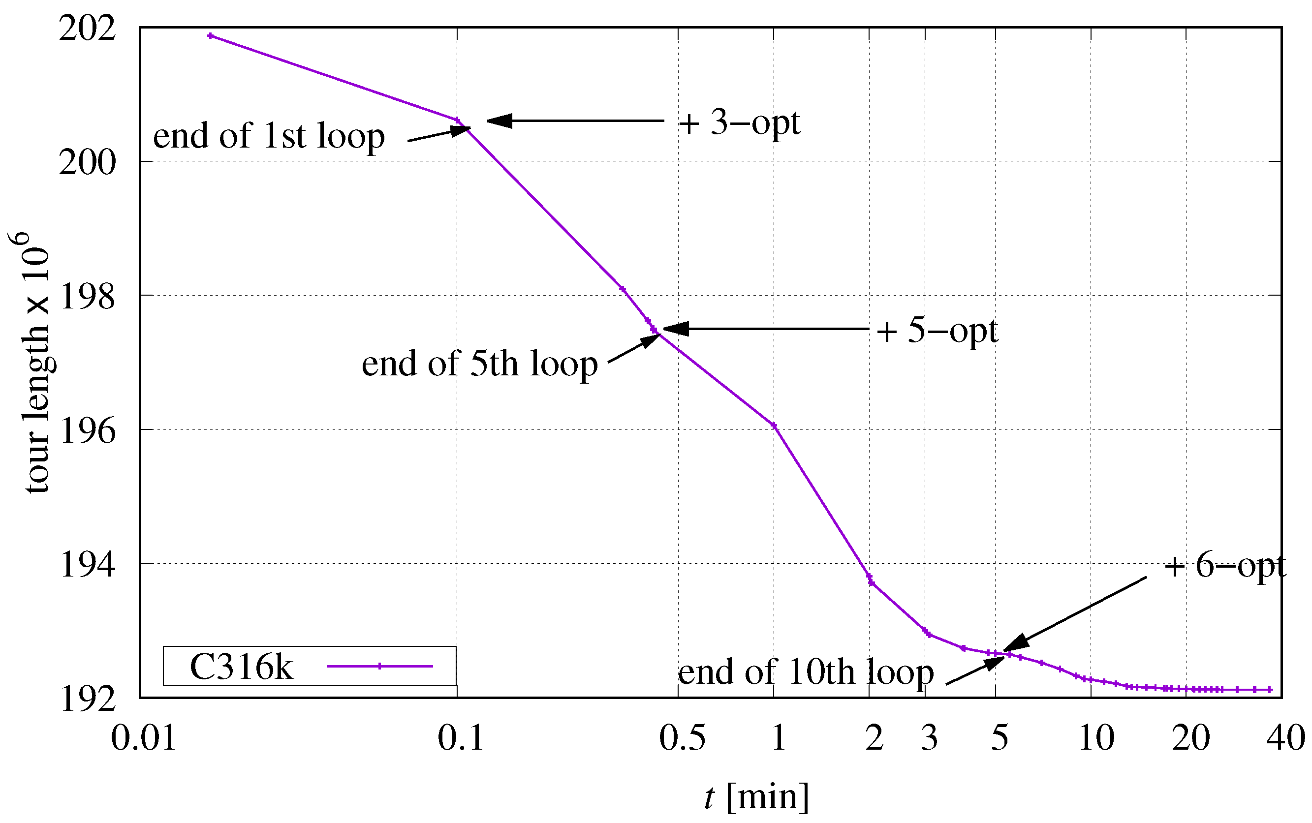
The general behaviour shall be illustrated by using the instance C316k.0. If other instances show different characteristics for certain settings, this will be mentioned explicitly. Candidate selection is restricted to the five closest candidates, the maximum edge distance between points Q and R is set to , parallel processing is turned off, and the one-level structure is used. Figure 8 shows the progress of optimization and marks special features.
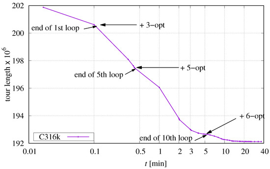
Figure 8.
Progress of optimization exemplified on instance C316k.0 and preliminary settings.
The initial tour with a length of 201 871 162 is provided by DoLoWire (30 s). After an initial loop over all points P using 2-opt permutations according to Section 2.4.1, the tour length is reduced to 200 615 308 by 3845 successful permutations. This reduction is possible because DoLoWire does not optimize the initial tour across cluster boundaries. Starting with the second loop, 3-opt operations (see Section 2.4.2) are also enabled. Table 9 represents the entire process in numbers. The time measurements have a precision of one second in all experiments.

Table 9.
Detailed information about the progress with respect to Figure 8.
With each loop, the number of successful permutations decreases until a certain threshold is reached. Then the next k-opt processing is activated and so on. The last loop simply verifies that no further improvement is possible and the processing terminates after about 37 min.
3.3. Investigations on Maximum Edge Distance
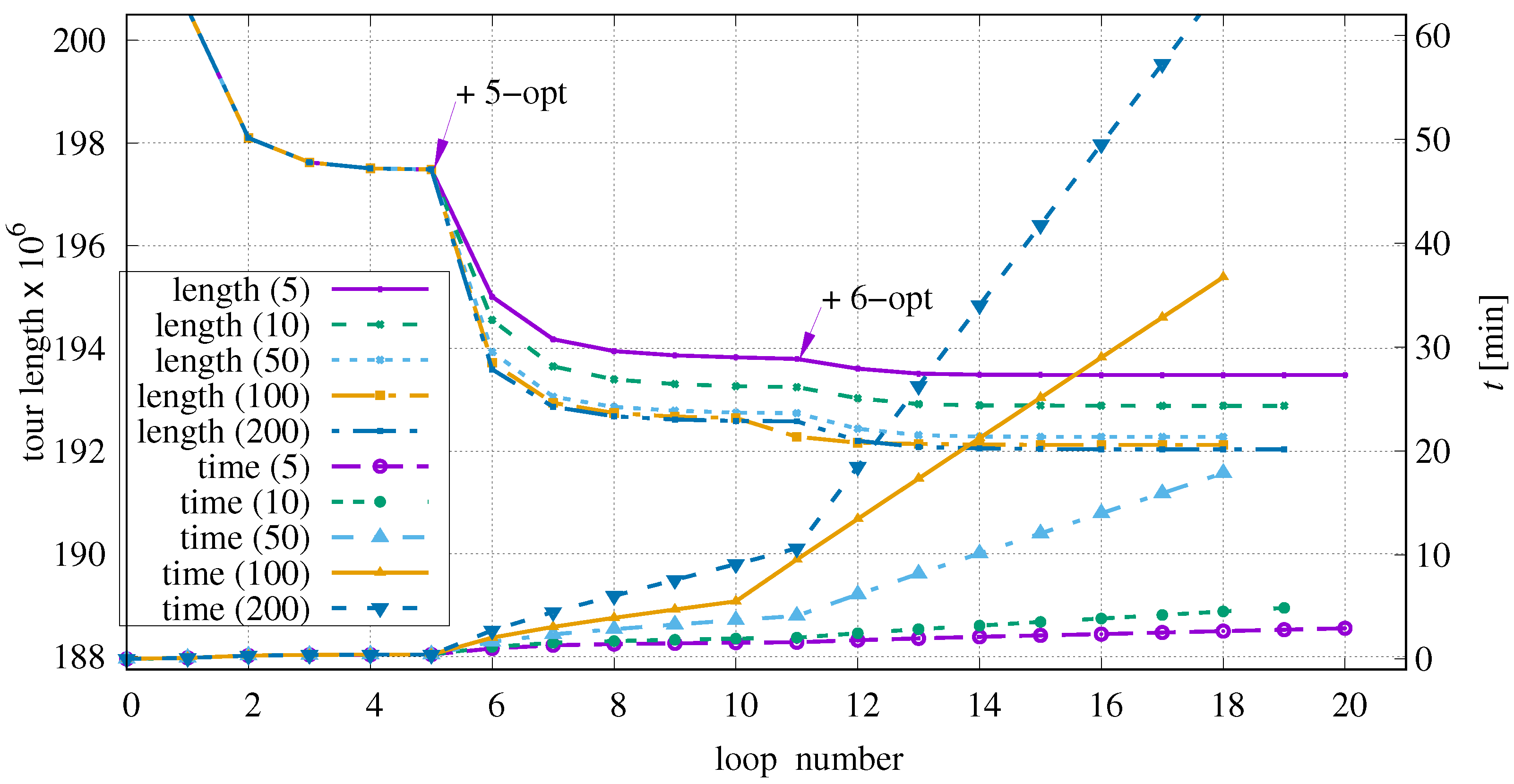
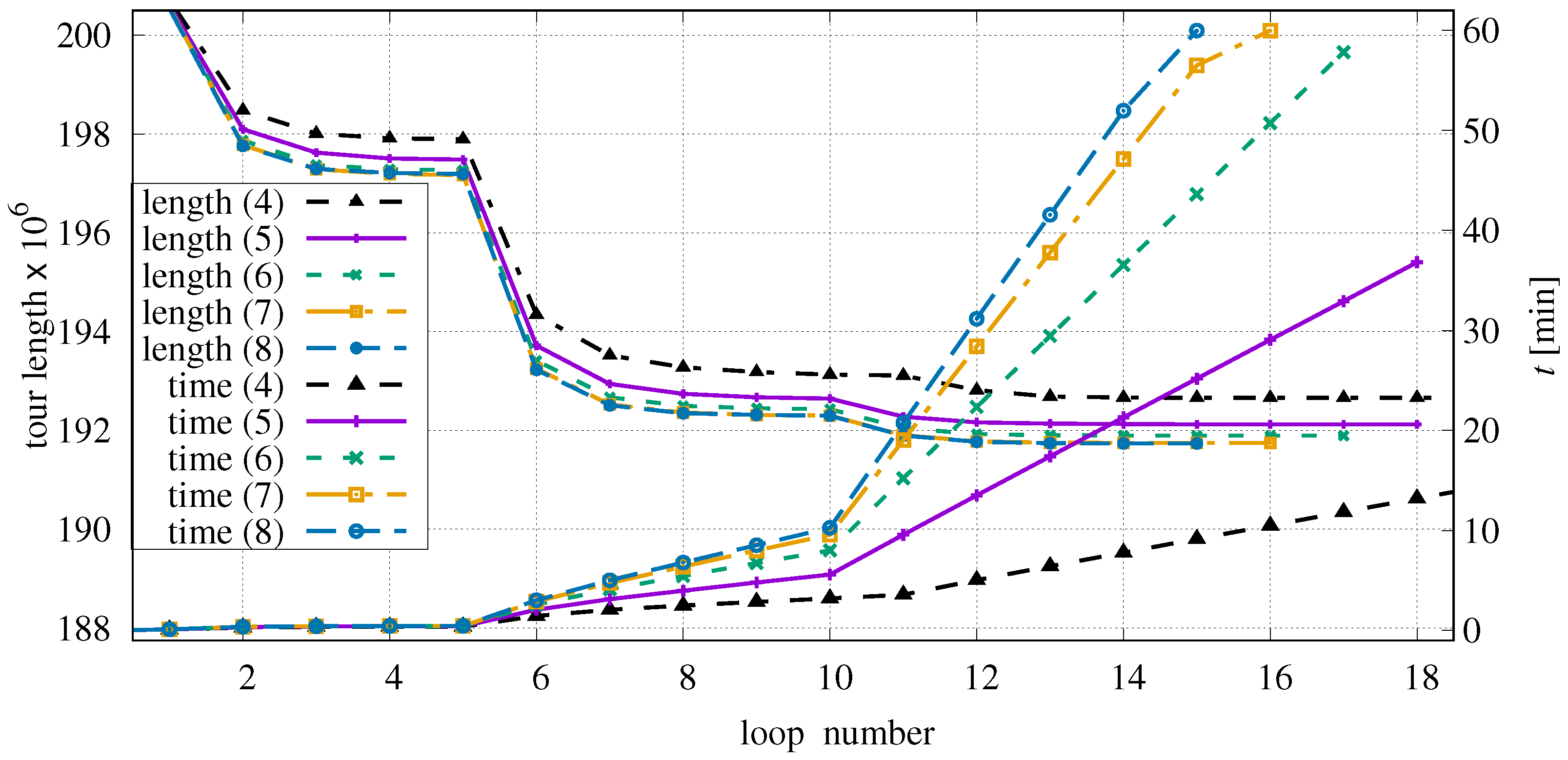
The number of points R to be examined depends on the chosen maximum edge distance between points Q and R. The variation of maxEdgeDist between 5 and 200 has been investigated. It affects the course of optimization and the time required to process each loop over P as can be seen in Figure 9.
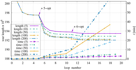
Figure 9.
Influence of maxEdgeDist exemplified on instance C316k.0.
For each parameter set, there are two curves depending on the loop number: one shows the current tour length and the other shows the elapsed time t.
The magenta curve () has two kinks at and . At these locations, the next k-opt permutations are activated. At the same loop positions, the time curve also has kinks because enabling more complex permutations increases the time needed for one loop over all P positions. Once the majority of successful permutations is performed, the duration per loop remains nearly constant until the set of enabled permutations is further expanded.
The smaller the maximum edge distance is chosen, the smaller the improvements per loop are, because some helpful permutations are not checked. At the same time, the duration per loop is shorter, i.e., the algorithm is faster. This leads to a flatter slope of the time curves and the optimizer can perform more loops in the same time. For very low values of maxEdgeDist, the optimization converges to unfavourable local minima. For example, with maxEdgeDist = 5, the algorithm stops after 20 loops, which are processed in three minutes; when using maxEdgeDist = 200, a local minimum is reached after 18 loops and approximately 73 min. Basically, we can see that the time needed to complete a certain loop is a function of maxEdgeDist, which is actually not a big surprise because the maxEdgeDist determines the number of inspected R positions (see Listing 2 line 10).
The behaviour within the first five loops is always the same because only 2-opt and 3-opt permutations are performed here, which do not depend on maxEdgeDist. Increasing maxEdgeDist from 100 to 200 only has a minor effect on the achieved improvements per loop. For other instances, it can be observed that values higher than rarely benefit the optimization process when using tight time constraints.
3.4. Investigations on Maximum Number of Candidates
In Table 1, it was shown that the average number of candidates is equal to six, when selected via Delaunay triangulation. The question is whether all candidates should always be considered or whether this set can be reduced to the nearest points.
Figure 10 shows the corresponding curves for and . In general, we observe that the performance improves when the number of candidates is increased up to . Choosing more than seven candidates has almost no effect on the tour length because only about 50% of all points have more than six candidates and the chance that a connection to one of the more distant candidates is favourable decreases. The processing time increases with , although this increase is only noticeable as long as there are points with at least candidates. Because the time limit was set to 60 min, the last loops of could not be completed leading to the kinks in the corresponding time curves.
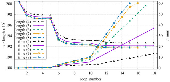
Figure 10.
Influence of maximum number of candidates exemplified on instance C316k.0.
3.5. Investigations on Data Structures
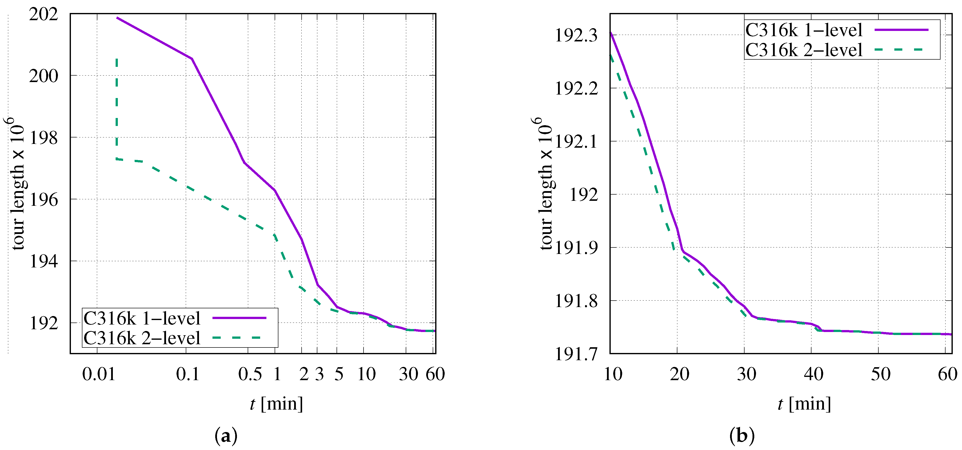
As described above, the simplest structure for storing point-order information is a permutation vector. This is considered a one-level structure. As an alternative, a two-level structure has been implemented, which is much more complicated from the point of view of data organisation, but it can reduce the required number of data accesses. Figure 11 shows the progress of optimization for TSP instance C316k (, ).
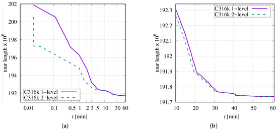
Figure 11.
Progress of optimization as function of time for C316k.0 and two alternative data structures: (a) over 60 min; (b) over last 50 min.
In the first few seconds, the tour length decreases much faster when using the two-level structure (see Figure 11a). This advantage persists beyond 10 min (see magnified diagram in Figure 11b).
Figure 12 illustrates the progress with respect to the number of performed loops over all positions P.

Figure 12.
Tour length as a function of each loop when optimizing C316k.0 in dependence on the used data structure and relative time of two-level data structure compared to one-level structure.
Loop zero corresponds the state after initial tour generation. The identical length curves prove that the achieved tour lengths are independent on the chosen data structure. That means both algorithms perform exactly the same sequence of permutations. Up to the fifth loop, the two-level structure requires only a tenth of the time compared to the one-level structure. This advantage vanishes when starting with 5-opt permutations. The positive effect of the two-level structure only becomes noticeable when many permutations can be applied. As soon as the optimization converges to a local minimum, the search for successful permutations takes more time than the actual permutations performed and the algorithmic overhead of the two-level structure consumes the time previously saved. After the 16th loop, the two-level structure has become slower on average than the one-level structure.
3.6. Investigations on Chosen Initial Tour Generator
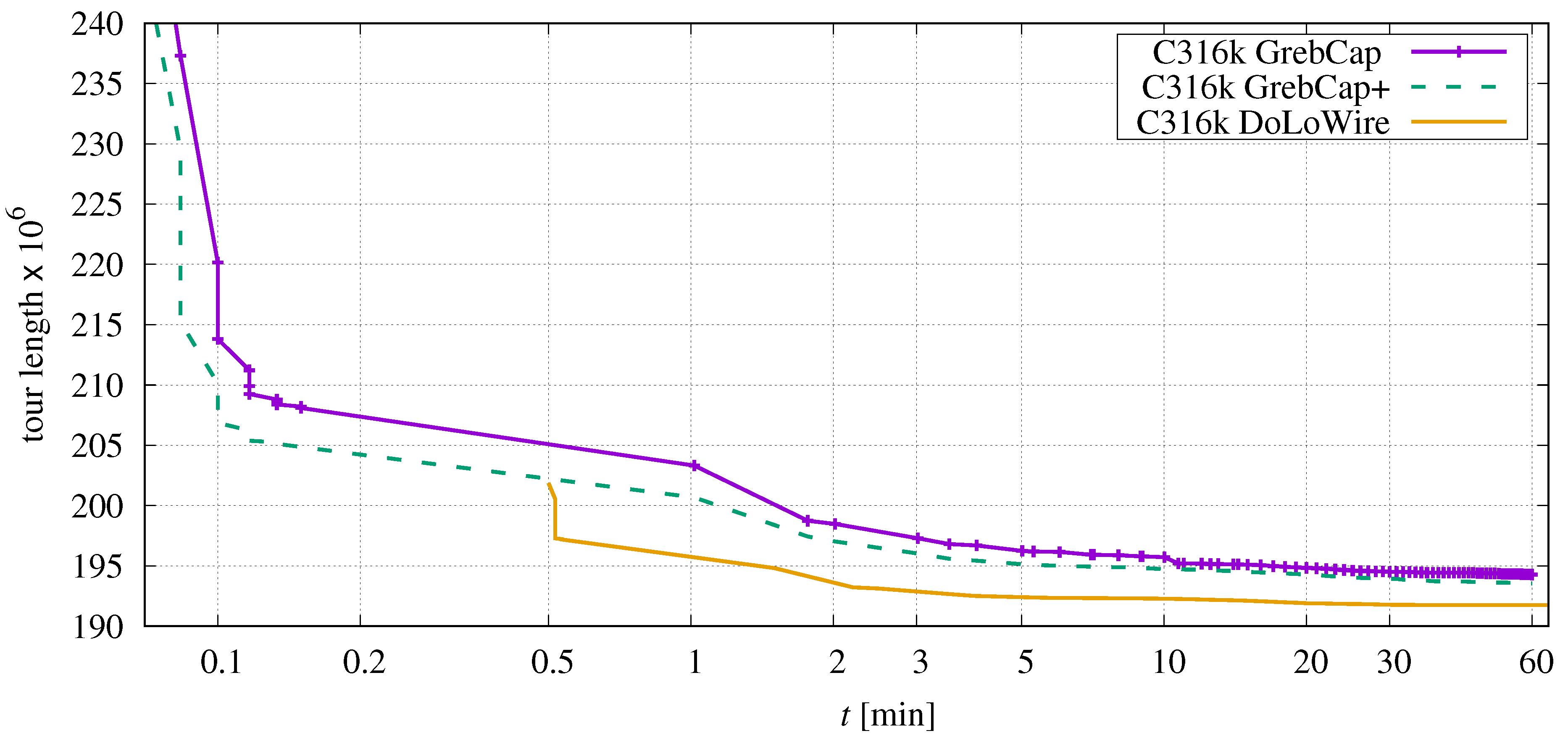
In Section 2.3, two different methods for generating an initial tour were discussed. The previous tests always relied on DoLoWire which creates much better tours than the GrebCap approach. It is now necessary to investigate what influence the quality of this initial tour has on the optimization process. Figure 13 depicts the progress as a function of time.
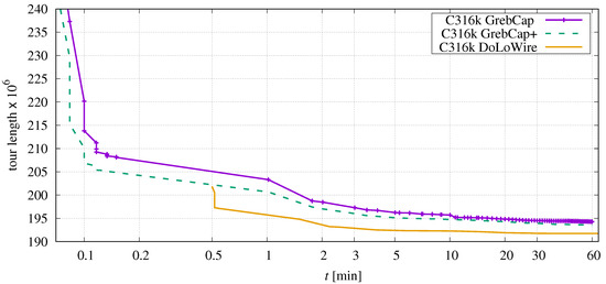
Figure 13.
Comparison of tour length depending on elapsed time when using different initial-tour generators applied to C316k.0.
In contrast to previous investigations, the elapsed time additionally includes the time needed for the initial tour generations. According to Table 2, this is 30 s for DoLoWire and about three seconds for the both GrebCap approaches. GrebCap+ denotes the greedy approach, including the candidate set enrichment and point merging (see Section 2.3.1).
It is obvious that the greedy approach produces an unfortunate initial tour. After 30 s of local optimization with Sys2to6, the tour is still worse than the result of the initialization by DoLowire and, moreover, the optimization converges to a worse local minimum.
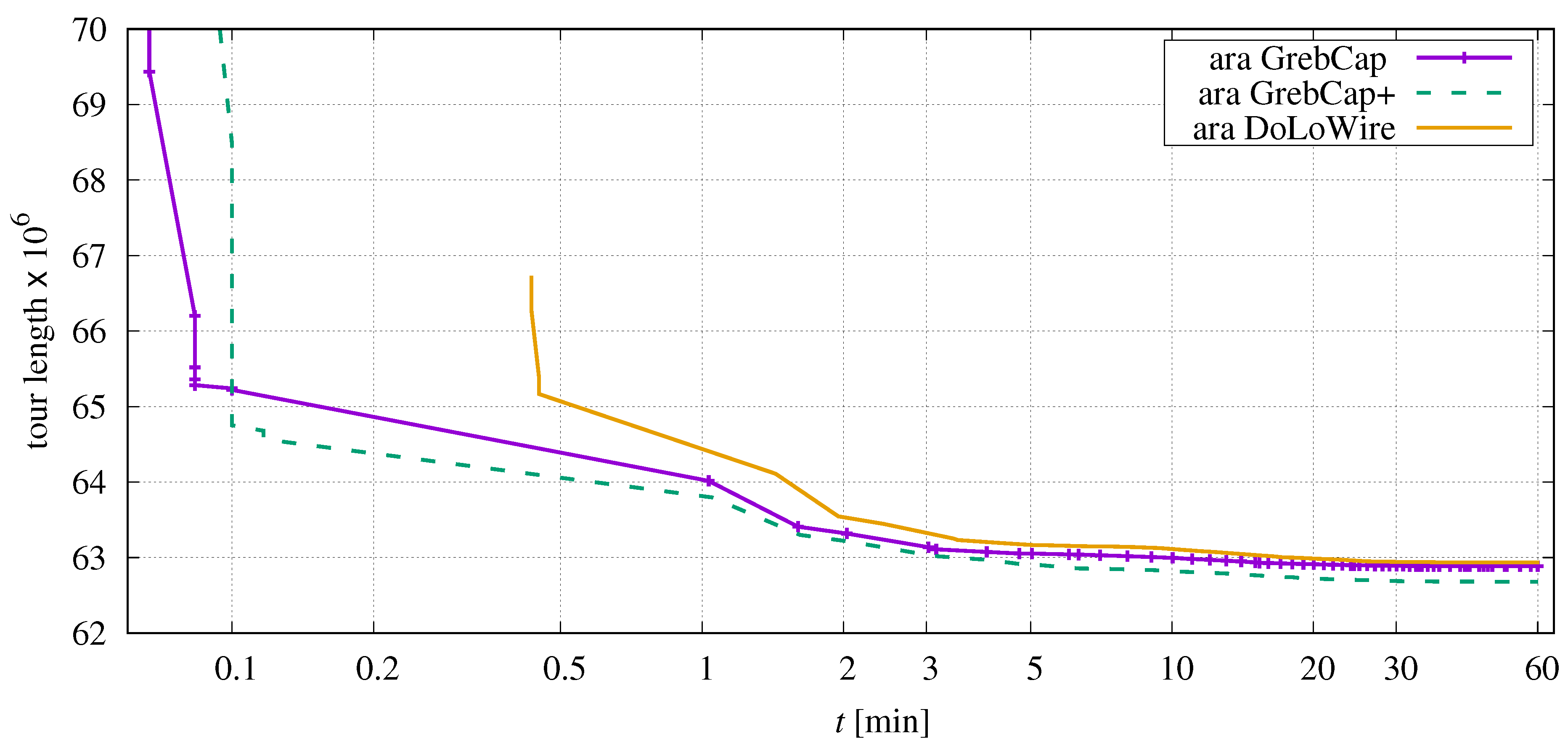
A different picture can be observed in application to ara238025.tsp, Figure 14.
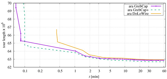
Figure 14.
Comparison of tour length depending on elapsed time when using different initial-tour generators in application to ara238025.tsp.
Here, the cluster-based generator of DoLoWire creates an unfortunate initial tour forcing the optimization process to a worse local minimum.
3.7. Parallel Processing of Tour Segments
As described in Section 2.5, the search for suitable permutations can be accelerated by parallelization. The influence of the number of parallel jobs on the course of the tour-length reduction has been investigated.
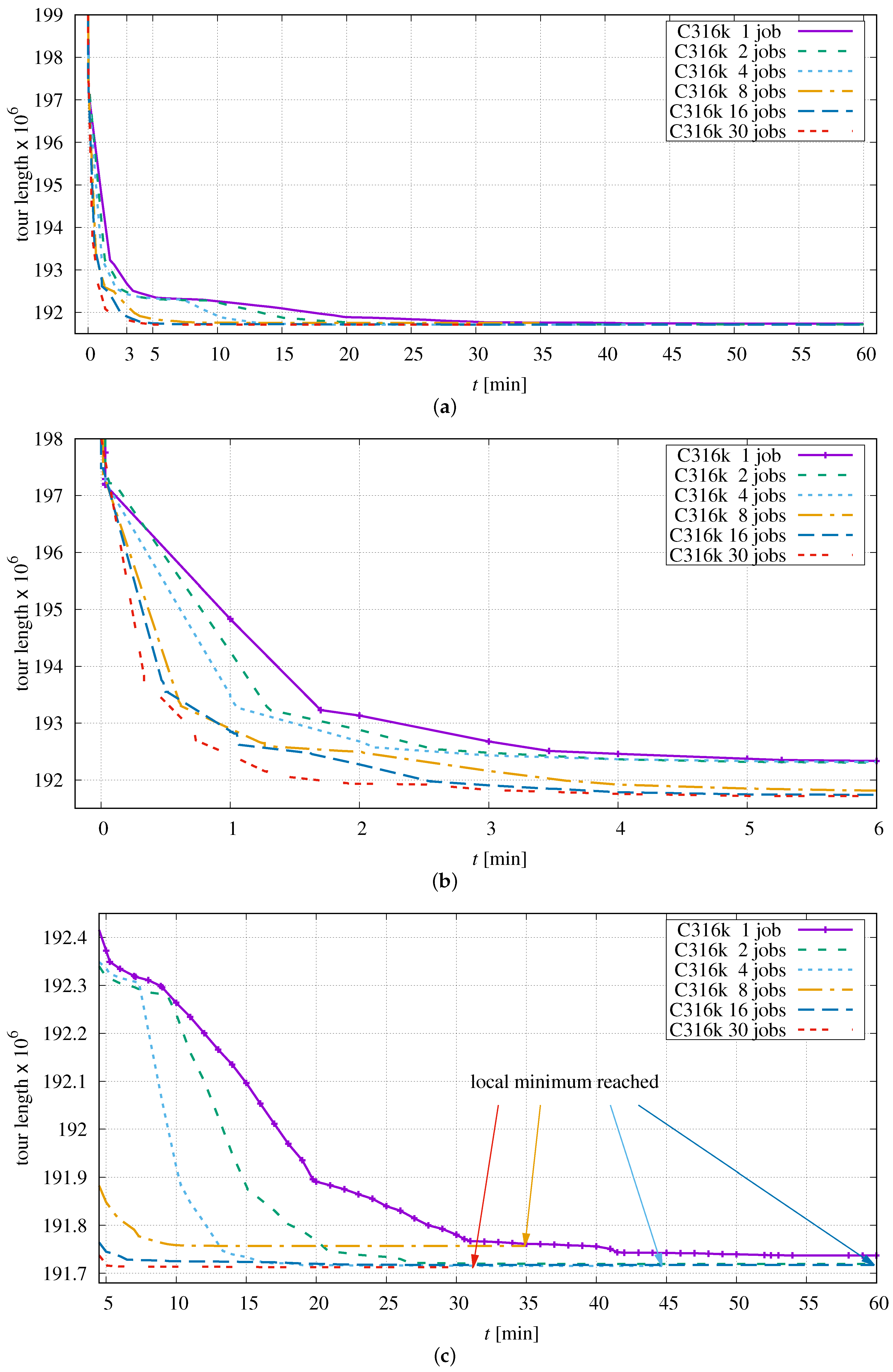
The results for C316k.0 are shown in Figure 15.
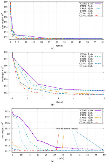
Figure 15.
Progress of optimization dependent on the number of parallel jobs in application to C316k.0: (a) over full duration, (b) first six minutes, (c) last 55 min.
The comparison now becomes somewhat more difficult because the order of permutations depends on the size of segments, which is, of course, a function of the chosen number of parallel jobs.
It can be clearly seen that the optimization process distinctly benefits from the use of multiple threads within the first three minutes (Figure 15a,b). After that, all variants converge to different local minima which is due to the varying order of permutations performed (Figure 15c). The maximum number of threads is set to 30 because the CPU has 32 physical cores. Two cores are reserved for background processes of the operating system so that they do not influence the time measurement too much.
By using at least eight parallel jobs for this instance, the local minimum can be reached within 60 min. With 30 jobs, the shortest tour can be attained after approximately half an hour. A similar minimum is obtained with 16 jobs, but in this example it takes almost 60 min to reach the point of convergence. When using eight parallel jobs, the minimum is reached after 35 min. Unfortunately, the sequence of permutations here steers the optimization into an unfavourable local minimum.
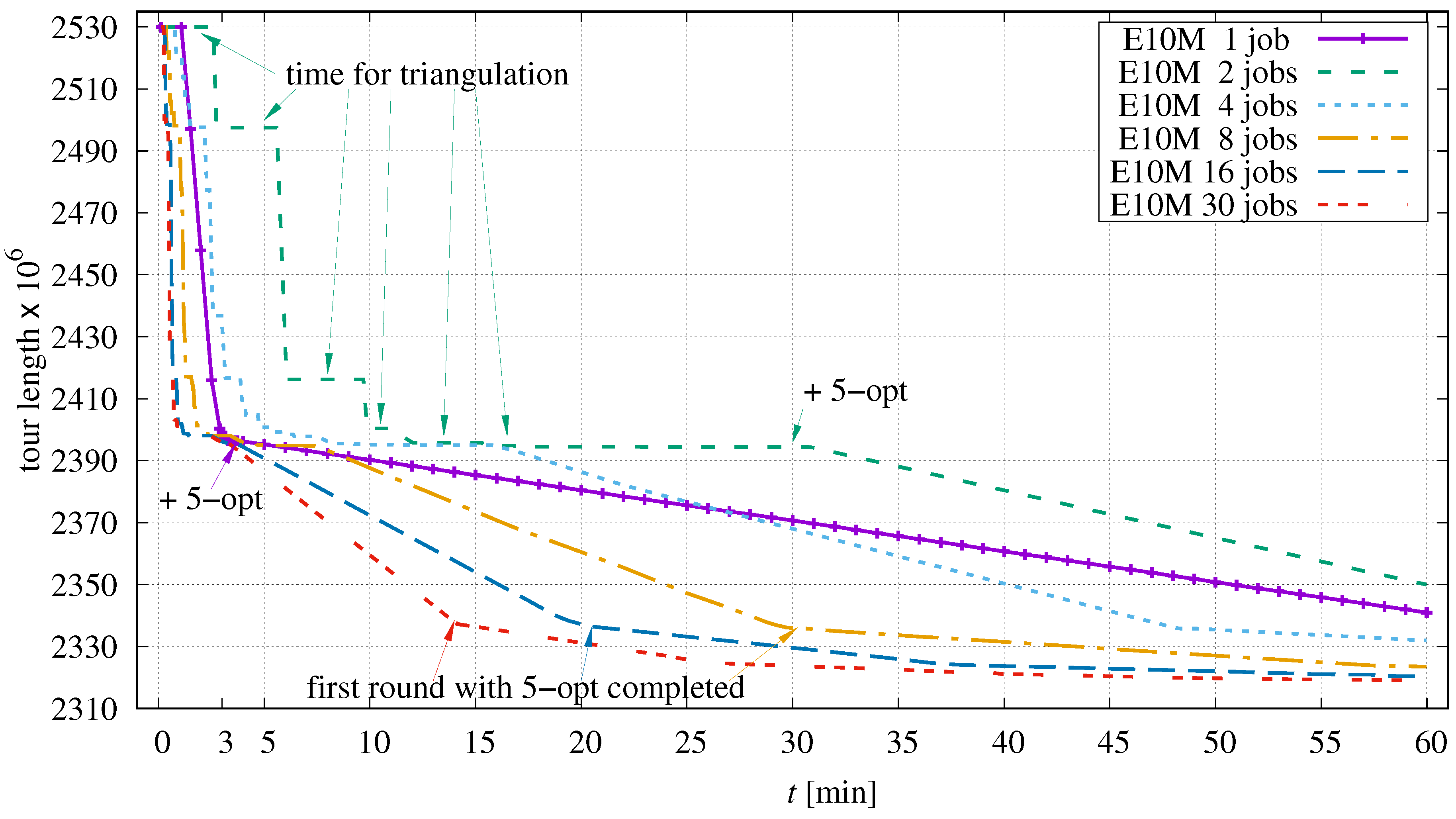
Most interesting is the influence of multithreading on the largest instance in the TSPs set used. Figure 16 depicts the optimization progress for E10M.0 containing ten million points as a function of the number of parallel jobs.
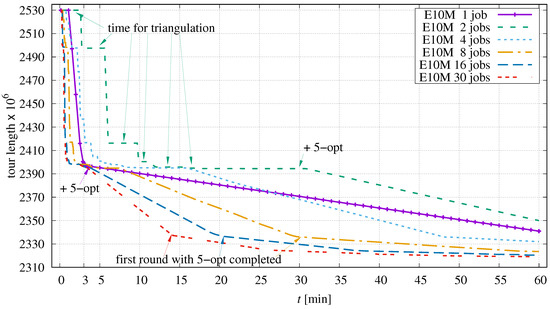
Figure 16.
Progress of optimization dependent on the number of parallel jobs in application to E10M.0.
The optimization starts with an initial tour of length 2 529 955 468 provided by DoLoWire. Reading the corresponding coordinates and permutation files takes eight seconds. For the single-job case (solid curve), the determination of candidates takes additional 61 s before the actual optimization can begin. When 2-opt and 3-opt permutations have exhausted their potential (after about 210 s), 5-opt operations are enabled. The tour is then steadily improved until the time limit is reached.
When using two parallel jobs, the preparation time increases to 150 s due to an unfortunate point configuration for the triangulation algorithm used. This computational overhead is needed after each round of parallel processing causing the stair-stepped curve up to about 11 min. The following plateau is a consequence of the chosen scheduling mechanism which switches back to single-job processing too early in this situation. After 30 min, the first round of parallel processing with 5-opt permutations is activated, and it continues until the specified time expires.
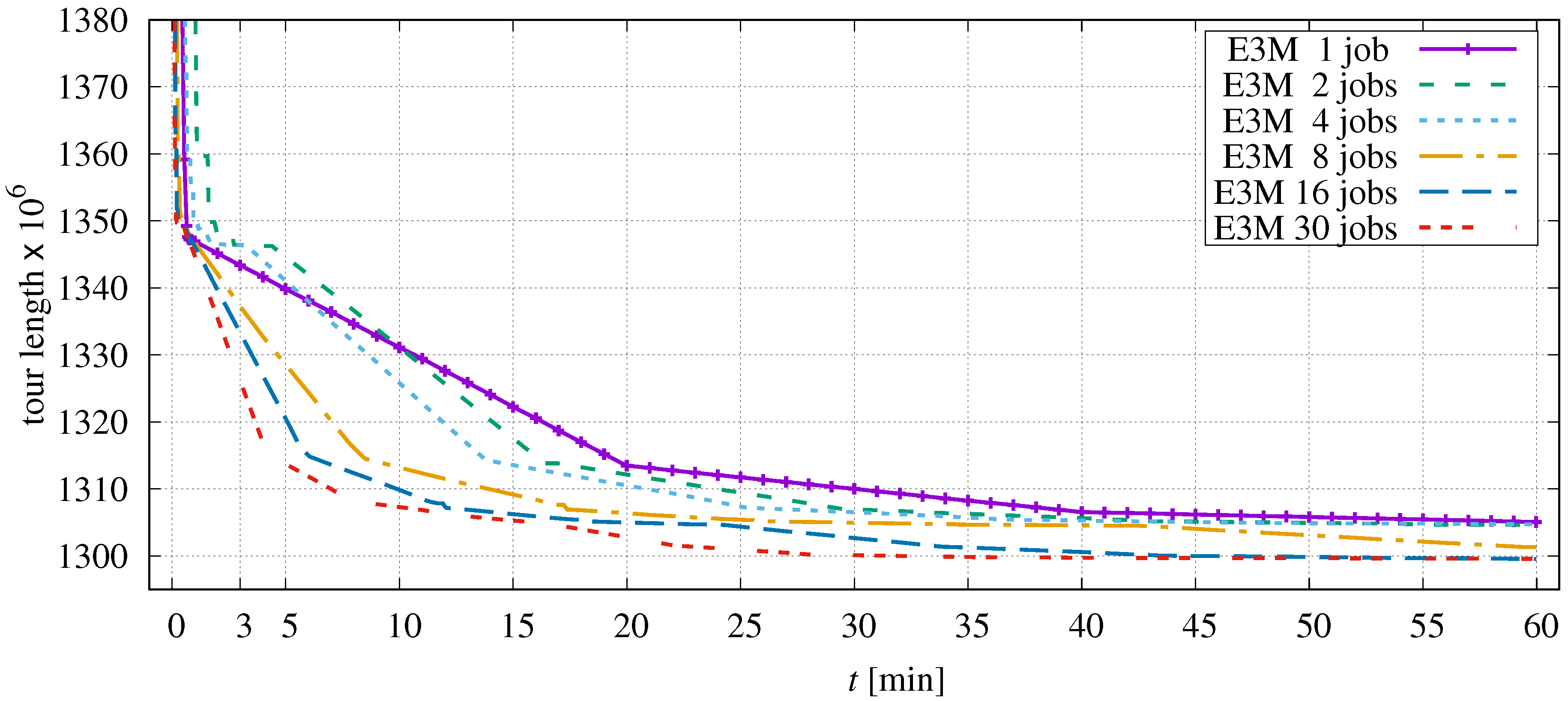
The more jobs are used in parallel, the fewer points are contained in each sequence, and the triangulation overhead becomes less pronounced. The curves now appear to be piecewise linear. This is simply a consequence of the uniform distribution of points in E10M.0. Each round of parallel processing corresponds to exactly one loop over all points P. The chance of improvement is evenly distributed in this course. With each new round, the probability of successful permutations decreases; the curves flatten accordingly. A similar progression is observed for E3M.0, the second largest instance of the test set (Figure 17).
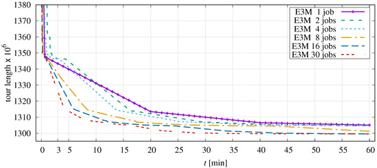
Figure 17.
Progress of optimization dependent on the number of parallel jobs in application to E3M.0.
The more segments are processed in parallel, the faster the tour length is improved.
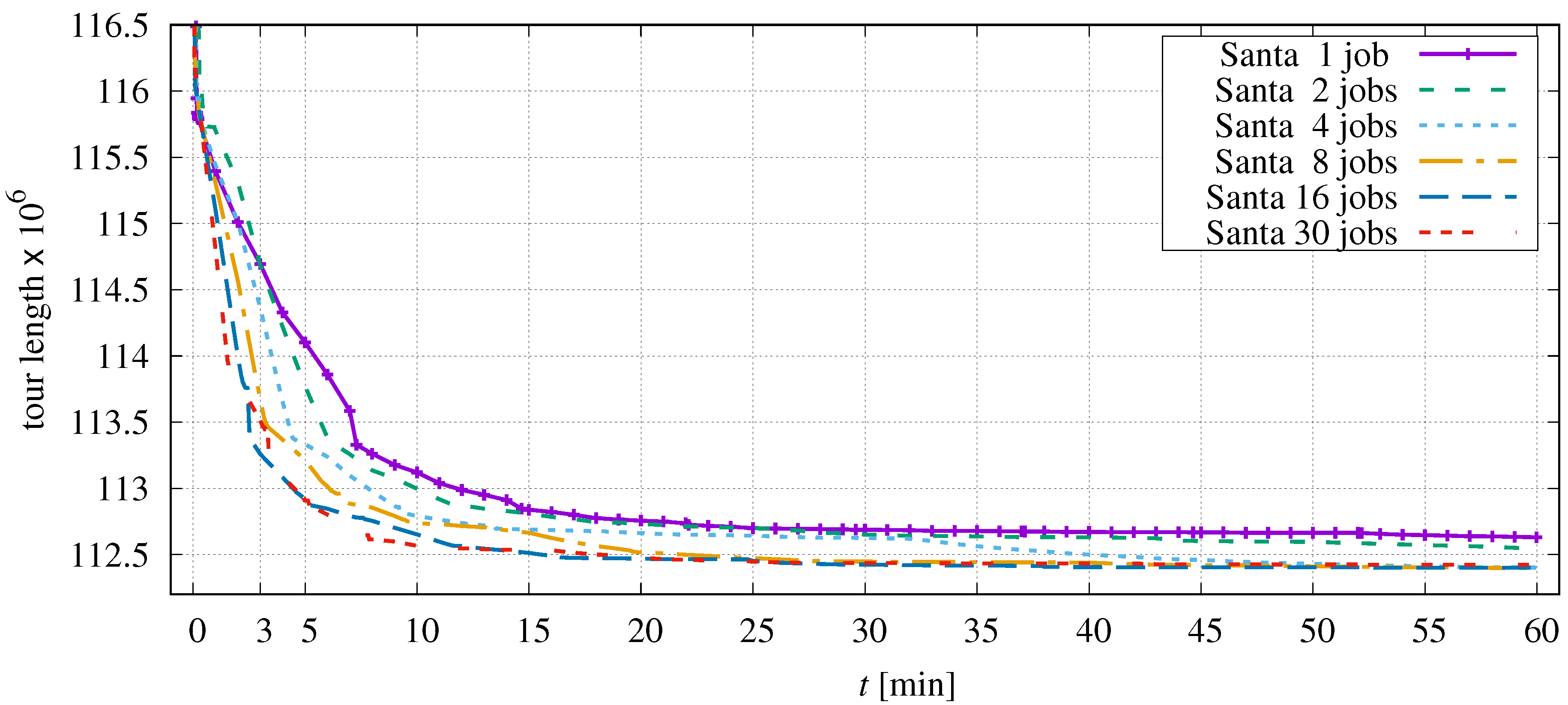
Optimizing the third-largest instance ‘santa1437195’ gives a slightly different picture. The curves in Figure 18 are less regular because the progress depends on the location of the points that are being processed.
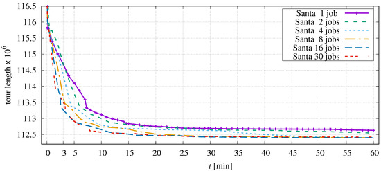
Figure 18.
Progress of optimization dependent on the number of parallel jobs in application to santa1437195.
This instance is highly clustered, and different parts of the tour have different optimization potential. Depending on the segmentation chosen, it is also possible that an unfortunate permutation is chosen which temporarily leads the optimization in an unfavourable direction. As can be seen for the 30-jobs curve, the tour length achieved after one hour is not significantly different from the result of the 16-job optimization. The advantage of two jobs over single-thread processing comes into play after about three minutes.
Based on the optimization progress, it can be observed that the acceleration of the improvements does not scale with the number of parallel jobs. Inspecting the plot of instance E3M.0 (Figure 17), the relation between number of jobs and required processing time t to reach a tour length of about is as follows:
Parallelization in 30 threads only leads to a fivefold increase in optimization speed. There are at least three reasons for this. First, there is some overhead in managing parallel processing, including candidate set generation. Secondly, the optimizer misses more and more favourable permutations as the segments to be processed become shorter. Third, and this is the main reason, parallel optimization often has to be interrupted by single-job processing to exchange information between distant segments (see Section 2.5.3).
3.8. Comparison with a State-of-the-Art Method
The proposed method Sys2to6 is now compared to LKH [56], which is widely known as a state-of-the-art heuristic for finding excellent TSP tours. The performance of Sys2to6 is mainly influenced by the values usedfor the number of candidates , the value, the number of parallel jobs, and the maximal duration of processing. The latter is set to a limit of 30 min (including the initial tour generation), in combination with . The other two parameters have been varied (, ). A good compromise could be found by using and . Note that without time constraints, larger values for both parameters would typically lead to shorter tours.
The default LKH settings are geared toward small and medium-sized instances. For large instances, the preparation of initial values already takes more than an hour even without outputting an initial tour. To force LKH to output results within 30 min also for E10M.0 requires special options (see Table 10).

Table 10.
Required parameter settings for LKH for solving large instances within half an hour.
The generation of sets of candidates by using the default settings is too time-consuming and must be replaced by the Delaunay method. The corresponding implementation enriches the set of Delaunay candidates as described in Section 2.3.1 with respect to Figure 3. Finally, the five Delaunay candidates with the smallest value are used [57]. It has to be mentioned that LKH can result in better tours for smaller instances when manually optimized settings are used.
The time limit is set to a maximum of 30 min. However, because LKH does not include preprocessing in the time measurement, this limit must be adaptively reduced for each instance. Because the initial tour generation of LKH is dependent on seeding the random number generator, the optimization process is started 10 times with different seed values bu using the keyword SEED. The average tour length is chosen for the comparison. Running LKH on instance Tnm100000 causes the program to abort. This can be prevented by additional use of the option ‘PRECISION = 1’ [57].
Table 11 compares the results in terms of final tour length obtained within 30 min of optimization.

Table 11.
Results for different instances after 30 min of processing. Values of column ’Best known length’ are copied from [58] for DIMACS (*.0) and from [59] for VLSI (*.tsp) instances. The best-known results for Tnm100000 and santa1437195 have been reported in [29] and [42], respectively.
When processing very large instances with LKH, it is not possible to get a tour-length value close to 30 min, the actual calculation times are about 32 min for E3M.0 and about 38 min for E10M.0.
The instances ExM.0 contain uniformly distributed points. As can be concluded from the results in Table 11, LKH does an excellent job for theses instances. The achieved excesses are less than 0.5% whereas the tours obtained with Sys2to6 are significantly longer. Something similar can be observed for the VLSI instances. Here, Sys2to6 performs worst with excess values above 8%.
For the instances Cxk.0, which contain many clusters of points, the proposed method can outperform LKH. The best performance of Sys2to6 in relation to LKH can be observed for the instance santa1437195. It contains 1 437 195 two-dimensional coordinates of households (Finnish National Coordinate System) distributed all over Finland (see for example [42]). These coordinates also show distinct clusters in large Finnish cities. With the given settings and constraints, LKH has problems dealing with this dataset, resulting in an excess of 7.32%, whereas Sys2to6 only has an excess of 3.69%.
As the performance of Sys2to6 might depend on the initial-tour generation chosen, additional investigations have been conducted by using GrebCap+ instead of DoLoWire. Taking the random component of GrebCap+ into account, the optimization has been performed 10 times for each instance. Table 12 lists the corresponding results in terms of worst, best, and median tour.

Table 12.
Results for different instances after 30 min of processing for Sys2to6 in combination with GrebCap+. Results in bold face are better than Sys2to6 in combination with DoLoWire.
In only three cases is the performance improved when using GrebCap+ instead of DoLoWire for initial tour generation. In addition, the tour lengths significantly increase for the clustered instances C100k, C316k, and santa1437195, which obviously benefit from using DoLoWire as initial tour generator.
The chosen settings , are a compromise between fast processing and large permutation search space with respect to the chosen time constraint. Additional investigations have shown that with respect to the limited time span of 30 min, the largest two instances in the studied set would benefit from smaller values for these two parameters, because the local improvements contribute more to the reduction of the tour length than the larger search space. Fine-granular modification of the parameters results in different optimal settings for different instances. This is mainly due to the modified order of permutation selection, which directs the optimization process to different region in the hyperspace of tour lengths.
4. Summary
A framework for the systematic application of k-opt permutation (), called “Sys2to6”, has been developed, implemented and studied with a focus on fast optimization progress for very large instances based on a single run. The objective was to find short tours within only 30 min. By using appropriate candidates and special arrangement of positions to cut the tour, the complexity of the search is kept at a feasible level.
The parallel processing of nonoverlapping tour segments accelerates the progress of optimization in the early stages before the entire process asymptotically approaches a local minimum. The same could be observed for the implemented two-level data structure. It is very helpful at the beginning of optimization when many permutations can be performed. In the long run of asymptotic convergence toward the local minimum, the ratio between number of successfully applied permutations and the number of inspected permutations is very small. The positive effect of faster permutations is consumed by the increased efforts required to access the two-level data structure. For optimization without time limitations, the implemented one-level data structure is preferable.
It could be shown that the proposed method can compete with a state-of-the-art approach based on the Lin–Kernigham method (LKH, [60]) within the investigated scenario. While LKH shows excellent performance for TSP instances with uniformly distributed points, Sys2to6 offers an advantage when dealing with clustered instances. Parallel processing of tour segments benefits optimization speed, but not to the extent desired. Other methods of parallelization should be considered. One possibility would be to run parallel full-tour optimizations with different starting points. As soon as one of the processes finds an improving permutation, all other processes are interrupted and restart with the new tour. This will be subject of future research.
Funding
This research received no external funding.
Data Availability Statement
Source code and investigated TSP instances are available at https://www.hs-coburg.de/fileadmin/fdm/tilo.strutz/Sys2to6-resources.zip, accessed on 7 December 2022.
Conflicts of Interest
The authors declare no conflict of interest.
References
- Der Handlungsreisende wie er Seyn Soll und Was er zu Thun Hat, um Aufträge zu Erhalten und Eines Glücklichen Erfolgs in Seinen Geschäften Gewiß zu Seyn; Voigt: Ilmenau, Germany, 1832.
- Menger, K. Das Botenproblem. In Ergebnisse Eines Mathematischen Kolloquiums; Dierker, E., Siegmund, K., Eds.; Springer: Berlin/Heidelberg, Germany, 1998; pp. 11–12. [Google Scholar]
- Applegate, D.L.; Bixby, R.E.; Chvátal, V.; Cook, W.J. The Traveling Salesman Problem: A Computational Study; Princeton University Press: Princeton, NJ, USA, 2007. [Google Scholar]
- Applegate, D.; Cook, W.J.; Rohe, A. Chained Lin-Kernigham for Large Traveling Salesman Problems. INFORMS J. Comput. 2003, 15, 82–92. [Google Scholar]
- Hougardy, S.; Zhong, X. Hard to solve instances of the Euclidean Traveling Salesman Problem. Math. Program. Comput. 2021, 13, 51–74. [Google Scholar]
- Helsgaun, K. General k-opt submoves for the Lin-Kernighan TSP heuristic. Math. Program. Comput. 2009, 1, 119–163. [Google Scholar]
- Christofides, N. Worst-Case Analysis of a New Heuristic for the Travelling Salesman Problem; Technical Report 388; Graduate School of Industrial Administration, Carnegie-Mellon University: Pittsburgh, PA, USA, 1976. [Google Scholar]
- van Bevern, R.; Slugina, V.A. A historical note on the 3/2-approximation algorithm for the metric traveling salesman problem. Hist. Math. 2020, 53, 118–127. [Google Scholar] [CrossRef]
- Arora, S. Polynomial-time approximation schemes for Euclidean TSP and other geometric problems. In Proceedings of the 37th Annual IEEE Symposium on Foundations of Computer Science, Burlington, VT, USA, 14–16 October 1996; pp. 2–12. [Google Scholar]
- Mitchell, J.S.B. Guillotine Subdivisions Approximate Polygonal Subdivisions: A Simple Polynomial-Time Approximation Scheme for Geometric TSP, k-MST, and Related Problems. SIAM J. Comput. 1999, 28, 1298–1309. [Google Scholar]
- Johnson, D.S.; McGeoch, L.A. Experimental analysis of heuristics for the STSP. In Traveling Salesman Problem and Its Variations; Gutin, G., Punnen, A.P., Eds.; Springer: Berlin/Heidelberg, Germany, 2002; pp. 369–443. [Google Scholar]
- Lin, S. Computer solutions of the Traveling Salesman Problem. Bell Syst. Tech. J. 1965, 44, 2245–2269. [Google Scholar]
- Lin, S.; Kernighan, B.W. An Effective Heuristic Algorithm for the Traveling-Salesman Problem. Oper. Res. 1973, 21, 498–516. [Google Scholar]
- Christofides, N.; Eilon, S. Algorithms for Large-scale Travelling Salesman Problems. J. Oper. Res. Soc. 1972, 23, 511–518. [Google Scholar] [CrossRef]
- Laporte, G. A concise guide to the Traveling Salesman Problem. J. Oper. Res. Soc. 2010, 61, 35–40. [Google Scholar] [CrossRef]
- Bektas, T. The multiple traveling salesman problem: An overview of formulations and solution procedures. Omega 2006, 34, 209–219. [Google Scholar] [CrossRef]
- Ochelska-Mierzejewska, J.; Poniszewska-Marańda, A.; Marańda, W. Selected Genetic Algorithms for Vehicle Routing Problem Solving. Electronics 2021, 10, 3147. [Google Scholar] [CrossRef]
- De Jaegere, N.; Defraeye, M.; Van Nieuwenhuyse, I. The Vehicle Routing Problem: State of the Art Classification and Review; Technical Report Research Report KBI-1415; KU Leuven—Faculty of Economics and Business: Leuven, Belgium, 2014. [Google Scholar]
- Abeledo, H.; Fukasawa, R.; Pessoa, A.; Uchoa, E. The time dependent traveling salesman problem: Polyhedra and algorithm. Math. Program. Comput. 2013, 5, 27–55. [Google Scholar]
- Hansknecht, C.; Joormann, I.; Stiller, S. Dynamic Shortest Paths Methods for the Time-Dependent TSP. Algorithms 2021, 14, 21. [Google Scholar] [CrossRef]
- Gutin, G.; Karapetyan, D. A memetic algorithm for the generalized traveling salesman problem. Nat. Comput. 2010, 9, 47–60. [Google Scholar]
- Laporte, G.; Palekar, U. Some applications of the clustered travelling salesman problem. J. Oper. Res. Soc. 2002, 53, 972–976. [Google Scholar] [CrossRef]
- Isoart, N.; Régin, J.C. A k-Opt Based Constraint for the TSP. In Proceedings of the 27th International Conference on Principles and Practice of Constraint Programming (CP 2021), Montpellier, France, 25–29 October 2021; Volume 210, pp. 30:1–30:16. [Google Scholar] [CrossRef]
- Baniasadi, P.; Ejov, V.; Filar, J.A.; Haythorpe, M.; Rossomakhine, S. Deterministic “Snakes and Ladders” Heuristic for the Hamiltonian cycle problem. Math. Program. Comput. 2014, 6, 55–75. [Google Scholar] [CrossRef]
- Krari, M.E.; Ahiod, B.; Benani, B.E. Breakout Local Search for the Travelling Salesman Problem. Comput. Inform. 2018, 37, 656–672. [Google Scholar]
- Jäger, G.; Dong, C.; Goldengorin, B.; Molitor, P.; Richter, D. A backbone based TSP heuristic for large instances. J. Heuristics 2014, 20, 107–124. [Google Scholar]
- Tinós, R.; Helsgaun, K.; Whitley, D. Efficient Recombination in the Lin-Kernighan-Helsgaun Traveling Salesman Heuristic. In Proceedings of the Parallel Problem Solving from Nature—PPSN XV—15th International Conference on Parallel Problem Solving from Nature, Coimbra, Portugal, 8–12 September 2018; Volume 1, pp. 95–107. [Google Scholar] [CrossRef]
- McMenemy, P.; Veerapen, N.; Adair, J.; Ochoa, G. Rigorous Performance Analysis of State-of-the-Art TSP Heuristic Solvers. In Evolutionary Computation in Combinatorial Optimization; Liefooghe, A., Paquete, L., Eds.; Springer: Cham, Switzerland, 2019; pp. 99–114. [Google Scholar]
- Skinderowicz, R. Improving Ant Colony Optimization efficiency for solving large TSP instances. Appl. Soft Comput. 2022, 120, 108653. [Google Scholar] [CrossRef]
- Xu, Q.; Guo, L.; Wang, N.; He, Y. COOBBO: A Novel Opposition-Based Soft Computing Algorithm for TSP Problems. Algorithms 2014, 7, 663–684. [Google Scholar] [CrossRef]
- Xu, S.; Wang, Y.; Huang, A. Application of Imperialist Competitive Algorithm on Solving the Traveling Salesman Problem. Algorithms 2014, 7, 229–242. [Google Scholar] [CrossRef]
- Dahan, F.; El Hindi, K.; Mathkour, H.; AlSalman, H. Dynamic Flying Ant Colony Optimization (DFACO) for Solving the Traveling Salesman Problem. Sensors 2019, 19, 1837. [Google Scholar] [CrossRef]
- Jedrzejowicz, P.; Wierzbowska, I. Parallelized Swarm Intelligence Approach for Solving TSP and JSSP Problems. Algorithms 2020, 13, 142. [Google Scholar] [CrossRef]
- Pacheco-Valencia, V.; Hernández, J.A.; Sigarreta, J.M.; Vakhania, N. Simple Constructive, Insertion, and Improvement Heuristics Based on the Girding Polygon for the Euclidean Traveling Salesman Problem. Algorithms 2020, 13, 5. [Google Scholar] [CrossRef]
- Zhang, Z.; Xu, Z.; Luan, S.; Li, X.; Sun, Y. Opposition-Based Ant Colony Optimization Algorithm for the Traveling Salesman Problem. Mathematics 2020, 8, 1650. [Google Scholar] [CrossRef]
- Mele, U.J.; Gambardella, L.M.; Montemanni, R. A New Constructive Heuristic Driven by Machine Learning for the Traveling Salesman Problem. Algorithms 2021, 14, 267. [Google Scholar] [CrossRef]
- Qamar, M.S.; Tu, S.; Ali, F.; Armghan, A.; Munir, M.F.; Alenezi, F.; Muhammad, F.; Ali, A.; Alnaim, N. Improvement of Traveling Salesman Problem Solution Using Hybrid Algorithm Based on Best-Worst Ant System and Particle Swarm Optimization. Appl. Sci. 2021, 11, 4780. [Google Scholar] [CrossRef]
- Sharma, S.; Chou, J. Accelerate Incremental TSP Algorithms on Time Evolving Graphs with Partitioning Methods. Algorithms 2022, 15, 64. [Google Scholar] [CrossRef]
- Taillard, É.D. A linearithmic heuristic for the travelling salesman problem. Eur. J. Oper. Res. 2022, 297, 442–450. [Google Scholar] [CrossRef]
- Zhang, J.; Hong, L.; Liu, Q. An Improved Whale Optimization Algorithm for the Traveling Salesman Problem. Symmetry 2021, 13, 48. [Google Scholar] [CrossRef]
- Fischer, T.; Merz, P. Reducing the size of traveling salesman problem instances by fixing edges. In Proceedings of the 7th European Conference on Evolutionary Computation in Combinatorial Optimization, Valencia, Spain, 11–13 April 2007; pp. 72–83. [Google Scholar]
- Strutz, T. Travelling Santa Problem: Optimization of a Million-Households Tour Within One Hour. Front. Robot. AI 2021, 8, 652417. [Google Scholar] [CrossRef]
- Yelmewad, P.; Talawar, B. Near Optimal Solution for Traveling Salesman Problem using GPU. In Proceedings of the 2018 IEEE International Conference on Electronics, Computing and Communication Technologies (CONECCT), Bangalore, India, 16–17 March 2018; pp. 1–6. [Google Scholar] [CrossRef]
- Delaunay, B. Sur la sphère vide. Bull. l’Académie Sci. l’URSS 1934, 6, 793–800. [Google Scholar]
- Croes, G.A. A method for solving traveling-salesman problems. Oper. Res. 1958, 5, 791–812. [Google Scholar]
- Helsgaun, K. An effective implementation of the Lin-Kernighan traveling salesman heuristic. Eur. J. Oper. Res. 2000, 126, 106–130. [Google Scholar]
- Helsgaun, K. An Effective Implementation of K-Opt Moves for the Lin-Kernighan TSP Heuristic; Technical report; Computer Science, Roskilde University: Roskilde, Denmark, 2006. [Google Scholar]
- Johnson, D. Local optimization and the Traveling Salesman Problem. In Proceedings of the International Colloquium on Automata, Languages, and Programming, ICALP 1990, England, UK, 16–20 July 1990; Volume 443, pp. 72–83. [Google Scholar] [CrossRef]
- Reinelt, G. Practical TSP Solving. In The Traveling Salesman: Computational Solutions for TSP Applications; Springer: Berlin/Heidelberg, Germany, 1994; pp. 200–210. [Google Scholar] [CrossRef]
- Xu, X.; Li, J.; Zhou, M. Delaunay-Triangulation-Based Variable Neighborhood Search to Solve Large-Scale General Colored Traveling Salesman Problems. IEEE Trans. Intell. Transp. Syst. 2021, 22, 1583–1593. [Google Scholar] [CrossRef]
- Fortune, S. A sweepline algorithm for Voronoi diagrams. Algorithmica 1987, 2, 152–174. [Google Scholar] [CrossRef]
- Perttunen, J. On the Significance of the Initial Solution in Travelling Salesman Heuristics. J. Oper. Res. Soc. 1994, 45, 1131–1140. [Google Scholar] [CrossRef]
- Fränti, P.; Nenonen, T.; Yuan, M. Converting MST to TSP path by branch elimination. Appl. Sci. 2021, 11, 177. [Google Scholar]
- Fredman, M.L.; Johnson, D.S.; McGeoch, L.A.; Ostheimer, G. Data Structures for Traveling Salesmen. J. Algorithms 1995, 18, 432–479. [Google Scholar]
- Strutz, T. Sys2to6 Optimization: Source Code and TSP Instances. 2023. Available online: https://www.hs-coburg.de/fileadmin/fdm/tilo.strutz/Sys2to6-resources.zip (accessed on 7 December 2022).
- Helsgaun, K. LKH-3 Version 3.0.6 (May 2019). 2019. Available online: http://webhotel4.ruc.dk/~keld/research/LKH-3/ (accessed on 7 December 2022).
- Helsgaun, K.; (Roskilde University, P.O. Box 260, DK-4000, Roskilde, Denmark). Private communication, 2022.
- Taillard, É.; Helsgaun, K. POPMUSIC for the Travelling Salesman Problem. Eur. J. Oper. Res. 2019, 272, 420–429. [Google Scholar] [CrossRef]
- University of Waterloo. VLSI Data Sets. 2022. Available online: https://www.math.uwaterloo.ca/tsp/vlsi/ (accessed on 7 December 2022).
- Helsgaun, K. Lin-Kernighan Heuristic Software. 2022. Available online: http://webhotel4.ruc.dk/~keld/research/LKH/LKH-2.0.10.tgz (accessed on 7 December 2022).
Disclaimer/Publisher’s Note: The statements, opinions and data contained in all publications are solely those of the individual author(s) and contributor(s) and not of MDPI and/or the editor(s). MDPI and/or the editor(s) disclaim responsibility for any injury to people or property resulting from any ideas, methods, instructions or products referred to in the content. |
© 2023 by the author. Licensee MDPI, Basel, Switzerland. This article is an open access article distributed under the terms and conditions of the Creative Commons Attribution (CC BY) license (https://creativecommons.org/licenses/by/4.0/).

