Improving Clustering Accuracy of K-Means and Random Swap by an Evolutionary Technique Based on Careful Seeding

Abstract

K-Means is a “de facto” standard clustering algorithm due to its simplicity and efficiency. K-Means, though, strongly depends on the initialization of the centroids (seeding method) and often gets stuck in a local sub-optimal solution. K-Means, in fact, mainly acts as a local refiner of the centroids, and it is unable to move centroids all over the data space. Random Swap was defined to go beyond K-Means, and its modus operandi integrates K-Means in a global strategy of centroids management, which can often generate a clustering solution close to the global optimum. This paper proposes an approach which extends both K-Means and Random Swap and improves the clustering accuracy through an evolutionary technique and careful seeding. Two new algorithms are proposed: the Population-Based K-Means (PB-KM) and the Population-Based Random Swap (PB-RS). Both algorithms consist of two steps: first, a population of $J$ candidate solutions is built, and then the candidate centroids are repeatedly recombined toward a final accurate solution. The paper motivates the design of PB-KM and PB-RS, outlines their current implementation in Java based on parallel streams, and demonstrates the achievable clustering accuracy using both synthetic and real-world datasets.

1. Introduction

Clustering is a fundamental machine learning [1] approach for extracting useful information from the data of such application domains as pattern recognition, image segmentation, text analysis, medicine, bioinformatics, and Artificial Intelligence. K-Means [2,3,4] is a classical clustering algorithm often used due to its simplicity and efficiency.

The aim of K-Means is to partition $N$ data points $X=\{x_i{\}}_{i=1}^N$, e.g., $x_i\in R^D$, in $K$, with $2\le K\ll N$, subsets (said clusters) by ensuring that points belonging to the same cluster are similar to one another, and points in different clusters are dissimilar. The Euclidean distance between data points usually expresses the similarity. Every cluster is represented by its central point or centroid. K-Means aims to optimize (minimize) the Sum-of-Squared Errors ($SSE$) cost, a sort of internal variance (or distortion) in clusters.

Recently, K-Means properties have been studied in depth [5,6,7]. A crucial aspect is the procedure which initializes the centroids (seeding method). In fact, the accuracy of a clustering solution strongly depends on the initial centroids. A basic limitation of K-Means is the adoption of a local strategy for managing centroids, which determines the algorithm often blocks in a sub-optimal solution. Random Swap [8,9] and genetic/evolutionary approaches [10,11,12] are examples of more sophisticated clustering algorithms that try to remedy this situation by adopting a global strategy of centroid management. At each iteration of Random Swap, a centroid is randomly selected and replaced by a randomly chosen data point of the dataset. The $SSE$ of the new configuration is then compared to that of the previous centroids’ configuration and, if it is diminished, the configuration becomes current for the next iteration. The algorithm can be iterated a maximum number of times. Random Swap has been demonstrated to approach, in many cases, the obtainment of a solution close to the optimal one, even with a possible increase in the computational time.

The contribution of this paper is the development of two new clustering algorithms by extending the K-Means and Random Swap through an evolutionary technique [10,13] and careful seeding. The two algorithms are Population-Based K-means (PB-KM) and Population-Based Random Swap (PB-RS). They borrow ideas from the evolutionary algorithms underlying GA-K-Means [10] and Recombinator-K-Means [11,12] and consist of two steps. In the first step, a population of candidate centroid solutions is initially built, by executing $J$ times the Lloyd’s K-Means or Random Swap along with the Greedy-K-Means++ (GKM++) [11,12,14] seeding method, which is effective for producing a careful configuration of centroids with a reduced $SSE$ cost. In the second step, PB-KM and PB-RS start from a configuration of centroids extracted by using GKM++ on the candidate centroids of the population. Then, they recombine centroids until a satisfying solution minimizes the $SSE$ cost.

The greater the number of repetitions is during the second step (independent restarts of PB-KM, the number of swap iterations of PB-RS), the higher the possibility of getting a combined solution near the best one is.

Regarding reliability and accuracy, PB-KM significantly enhances the classical Lloyd’s repeated K-Means in globular, spherical, and Gaussian-shaped clusters [5,6]. PB-RS is better suited for studying general datasets with an irregular distribution of points. A common issue of PB-KM and PB-RS, though, is the assumption that good clustering follows by minimizing the $SSE$ cost. Unfortunately, this is not true for some challenging datasets [9] which can only be approximated through the proposed and similar tools.

To cope with large datasets, PB-KM and PB-RS systematically use parallel computing. Currently, the two algorithms are developed in Java using lambda expressions and parallel streams [15,16]. This way, it is possible to exploit today’s multi/many-core machines transparently.

This paper extends the preliminary paper [17] presented at the Simultech 2023 conference, where the basic idea of PB-KM was introduced. Differences from the conference paper are indicated in the following.

• A more complete description of the evolutionary approach, which is the basis of the proposed clustering algorithms, is provided.
• PB-KM now includes a mutation operation in the second step of recombination.
• An original development of PB-RS is presented which, with respect to standard Random Swap [8,9], is more apt to move directly to a good clustering solution.
• More details about the Java implementations are furnished.
• All previous execution experiments were reworked, and new challenging case studies were added to the experimental framework, exploiting synthetic (benchmark) and real-world datasets.

The paper first describes the evolutionary approach of PB-KM and PB-RS, then reports the experimental results of applying them to several datasets. The simulation results confirm that the new algorithms can ensure accurate clustering and good execution times.

The paper is structured as follows. Section 2 reviews the related work about the K-Means and methods for seeding. It also overviews the fundamental aspects of Random Swap, the evolutionary clustering of GA-K-means and Recombinator-K-Means, which inspired the algorithms proposed here. The section also describes some external measures suited to assess the clustering quality. The operations of the PB-KM and PB-RS algorithms are presented in Section 3. Some implementation issues in Java are discussed in Section 4. Section 5 reports the chosen experimental setup made up of synthetic datasets and real-world ones, and the experimental results tied to the practical applications of the developed tools. The execution performance of the new algorithms is also demonstrated. Finally, conclusions are drawn together with an indication of ongoing and future work.

2. Related Work

This section provides a review of the clustering concepts and operation of K-Means [2,3,4,7], Genetic K-Means (GA-K-Means) [10], Random Swap [8,9] and the evolutionary Recombinator-K-Means [11,12], which are at the basis of the development of the two algorithms this paper proposes.

2.1. Lloyd’s K-Means

Algorithm 1 illustrates the operation of classical K-Means. In step 1, the data points of the dataset to assume as the initial centroids are established by a seeding procedure (e.g., uniform random, see also Table 1 of basic notations).

Table 1. Basic notations.

Symbol	Description
$N$	$\mathrm{number} \mathrm{of} \mathrm{data} \mathrm{points} \left(\mathrm{vectors}\right) x_i$$\mathrm{in} \mathrm{the} \mathrm{dataset} X$
$D$	number of dimensions (coordinates or features) for each data point
$K$	number of clusters/centroids
$d(x_i,x_j)$	$\mathrm{Euclidean} \mathrm{distance} \mathrm{between} \mathrm{data} \mathrm{points} x_i$$\mathrm{and} x_j$
$C_1\dots C_K$	partition clusters
${\mu }_1\dots {\mu }_K$	representative centroids of clusters
$nc\left(x_i\right)$	$\mathrm{nearest} \mathrm{centroid} \mathrm{to} \mathrm{data} \mathrm{point} x_i$
$L$	the number of currently defined centroids in a seeding method
$D\left(x_i\right)$	$\mathrm{minimal} \mathrm{distance} \mathrm{of} x_i$ to the currently existing centroids
$SSE$	Sum-of-Squared Errors objective function
$nMSE$	$\mathrm{normalized} \mathrm{mean} \mathrm{of} SSE$, also referred to as distortion
$Unif$	uniform random seeding method
$KM$++	K-Means++ seeding method
$GKM$++	Greedy-K-Means++ seeding method
$S$	number of attempts in GKM++ for identifying the next centroid
$CI$	Cluster Index—an external measure of clustering accuracy
<$C^j,P^j$>	a solution of a clustering algorithm, i.e., a pair of a centroids vector and corresponding partition labels of clusters belonging data points
$PB-KM$	proposed Population-Based K-Means clustering algorithm
$PB-RS$	proposed Population-Based Random Swap clustering algorithm
℘	$\mathrm{population} \mathrm{of} J\ast K$ centroids in PB-KM/PB-RS algorithms
$J$	number of “best” solutions initially put in the ℘
$R_1$	number of repetitions of K-Means in the 1st step of PB-KM
$R_2$	number of repetitions of K-Means in the 2nd step of PB-KM
$T$	number of iterations of Random Swap in the 1st step of PB-RS, for defining each of the J candidate population solutions; also the number of iterations of Random Swap in the 2nd step of PB-RS for achieving a careful solution

In step 2, the data points are partitioned according to current centroids. In particular, each point $x_i$ is assigned to the cluster $C_j$, of which the representative centroid, ${\mu }_j$, is nearest to$x_i$:

$${\mu }_j=nc\left(x_i\right), j={argmin}_{1\le h\le K}\left(d\left(x_i,{\mu }_h\right)\right)$$

where $d\left(x_i,{\mu }_h\right)$ expresses the Euclidean distance between $x_i$ and ${\mu }_h$ data points. In step 3, centroids get updated as the mean of the clusters’ belonging points:

$${{\mu }^{\prime }}_j=\frac{1}{\left|C_j\right|}\sum _{x_i\in C_j}{x}_i$$

Steps 2 and 3 are re-executed until a stop condition holds. For example, when the updated centroids $\{{{\mu }^{\prime }}_j{\}}_{j=1}^K$ practically “coincide” (according to a certain numeric tolerance) with the previous ones $\{{\mu }_j{\}}_{j=1}^K,$ the K-Means exits for reached convergence, otherwise, the stop condition occurs after the maximum number of iterations of steps 2 and 3 is finished. In any case, the new centroids $\{{{\mu }^{\prime }}_j{\}}_{j=1}^K$ become the current centroids, $\{{\mu }_j{\}}_{j=1}^K$.

Algorithm 1. The Lloyd’s K-Means

Input: the dataset $X$ and the number of clusters $K$. Output: final centroids and corresponding partitions. 1. Initialization. Use some seeding method (e.g., uniform random) to choose $K$ data in $X$ as initial centroids. 2. Partitioning. Assign data points of $X$ to clusters according to the nearest centroid rule. 3. Update. Redefine centroids as the mean points of the clusters resulting from step 2. 4. Check termination. If the termination condition does not hold, repeat from 2.

The goal of K-Means is minimizing the $SSE$ cost:

$$SSE={\sum }_{j=1}^K{\sum }_{x_i\in C_j }{d(x_i,{\mu }_j)}^2 \mathrm{with} {\mu }_j=nc\left(x_i\right)$$

In the practical case, the normalized mean value of $SSE$, named $nMSE$ and here also referred to as the distortion index, can be used (see Table 1):

$$distortion=nMSE=\frac{SSE}{N\ast D}$$

In general, optimizing the $SSE \left(\mathrm{o}\mathrm{r} \mathrm{t}\mathrm{h}\mathrm{e} distortion\right)$ function cost is very difficult. This is due to the highly non-convex character of the $SSE$. In addition, a good clustering of some datasets does not necessarily follow from the minimization of the $SSE$ (see, e.g., [9]). Therefore, clustering solutions are usually approximations of the optimal solution.

2.2. The Random Swap Clustering Algorithm

The behavior of K-Means is heavily dependent on its initial seeding. Centroid points are then subsequently refined locally. The global movement of centroids is, in many cases, forbidden. For example, the seeding procedure can sometimes associate multiple centroids with the same big real cluster, which is in turn well-separated from smaller clusters with no centroid associated with them. Consequently, the big cluster can get wrongly split into multiple sub-clusters because its centroids cannot move to smaller clusters without a centroid. This bad situation is favored when the two kinds of clusters are far away from each other [6]. What could help is the adoption of a global strategy governing the movement of centroids.

Random Swap [8] is a clustering algorithm based on such a global strategy. It starts by defining initial centroids via uniform random seeding. After that, it executes a certain number of swap iterations. At each swap, a centroid is randomly chosen in the vector of centroids, which is then replaced by a random point selected in the dataset:

$$c_s \leftarrow x_i , s=unif\_rand\left(1..K\right), i=unif\_rand(1..N)$$

In the case the resultant centroid configuration, preliminarily refined by a few K-Means iterations (e.g., 5), has an $SSE$ cost lesser than the previous configuration, it is accepted as the new current solution and the algorithm goes on by starting the next swap iteration. The previous configuration and associated partitioning are otherwise restored, and the new swap is launched. The algorithm terminates when the required maximum number of iterations are executed.

Given its modus operandi, Random Swap is naturally capable of exploring all the data space and ending up, in many practical cases [9], with a clustering solution close to the optimal one, provided an adequate number of iterations are executed.

2.3. Centroids Initialization Methods

As has been pointed out, e.g., in [5,6,7], initial centroids should be defined in such a way to not coincide with outliers or noise data points. In addition, centroids should be far away from one another. This requirement avoids splitting a big real cluster into multiple smaller clusters. Different seeding methods for the initialization of centroids are defined in the literature. A few of these methods are described in the following.

$Unif$. The uniform random seeding is the default method K-Means and Random Swap use. Centroids are initialized through a uniform random selection of $K$ distinct points of the dataset $X$:

$$\{{\mu }_j\leftarrow x_i, i=unif\_rand(1..N){\}}_{j=1}^K$$

$Unif$ is simple to apply, but it does not guarantee the properties mentioned above of centroids are fulfilled. Only when centroids are selected near the optimal positions, the clustering solution delivered by K-Means locates close to the optimal one. Consequently, using K-Means with $Unif$ seeding typically requires the algorithm to be repeated a certain number of times (Repeated K-Means or K-Means with Restarts). The more the independent repetitions are, the higher the chance of finding a solution near the optimal one is. In any case, if $R$ are the repetitions of the K-Means, the solution that minimizes the $SSE$ objective cost is identified as the “best” one among the $R$ runs.

Let, in the following, $D\left(x_i\right)$ be the minimal distance of point $x_i$ from the currently defined $L$ centroids, $1\le L\le K$.

$Maximin.$ The first centroid is established by selecting a point in the dataset by uniform random. Each subsequent centroid is a point $x_i\in X$ with maximal $D\left(x_i\right)$ from the currently defined centroids. The method is continued until all the $K$ centroids are defined. Similarly to K-Means++ (see below), the method tends to define centroids far away from one another and with a similar linear computational cost ($O\left(KND\right)$).

K-Means++. This seeding method [18] initializes centroids incrementally and probabilistically, as shown in Algorithm 2.

Algorithm 2. The K-Means++ seeding method.

1. Establish the first centroid through a uniform random selection:

${\mu }_1\leftarrow x_j, j\leftarrow unif\_rand(1..N), L\leftarrow 1$

2. For each point $x_{i },$ define the probability $\pi \left(x_i\right)$ of being chosen as the next centroid as:

$\pi \left(x_i\right)=\frac{{D\left(x_i\right)}^2}{{\sum }_{j=1}^N{{D(x}_j)}^2}$

Use a random switch based on the newly computed values of $\{\pi \left(x_i\right){\}}_{i=1}^N$, for choosing a  point $x^{*}\in X$, not previously selected, as the next centroid

$L\leftarrow L+1, { \mu }_L\leftarrow x^{*}$

3. If $L<K$, repeat from step 2.

K-Means++ is known to be a good seeding method. It tends to distribute the centroids in the data space more evenly, ensuring that they are located far away from each other.

$Greedy K$-Means++. This method is a refinement of K-Means++ [11,12,14]. Its operation is illustrated in Algorithm 3.

Algorithm 3. The Greedy_K-Means++ (GKM++) seeding method.

${\mu }_1\leftarrow x_j, j\leftarrow unif\_rand(1..N)$, $L\leftarrow 1$ $do\{$   $\mathrm{c}\mathrm{o}\mathrm{s}\mathrm{t}\mathrm{B}\mathrm{e}\mathrm{s}\mathrm{t}\leftarrow \mathrm{\infty }$   $\mathrm{c}\mathrm{a}\mathrm{n}\mathrm{d}\mathrm{B}\mathrm{e}\mathrm{s}\mathrm{t}\leftarrow ?$   $repeat S times \{$      $\mathrm{s}\mathrm{e}\mathrm{l}\mathrm{e}\mathrm{c}\mathrm{t}$ a point $x^{*}\in X$ as candidate centroid, using the K-Means++ method      $\mathrm{p}\mathrm{a}\mathrm{r}\mathrm{t}\mathrm{i}\mathrm{t}\mathrm{i}\mathrm{o}\mathrm{n}$ $X$ according to $\left\{{\mu }_1, {\mu }_2,\dots , {\mu }_L,x^{*}\right\},$that is assign points to clusters according      to the $nc\left(.\right)$ function      $\mathrm{c}\mathrm{o}\mathrm{s}\mathrm{t}\leftarrow SSE\left(\right)$      $if(\mathrm{c}\mathrm{o}\mathrm{s}\mathrm{t}<\mathrm{c}\mathrm{o}\mathrm{s}\mathrm{t}\mathrm{B}\mathrm{e}\mathrm{s}\mathrm{t}) \{$        $\mathrm{c}\mathrm{a}\mathrm{n}\mathrm{d}\mathrm{B}\mathrm{e}\mathrm{s}\mathrm{t}\leftarrow x^{*}$        $\mathrm{c}\mathrm{o}\mathrm{s}\mathrm{t}\mathrm{B}\mathrm{e}\mathrm{s}\mathrm{t}\leftarrow \mathrm{c}\mathrm{o}\mathrm{s}\mathrm{t}$      $\}$   $\}$   $L\leftarrow L+1$   ${\mu }_L\leftarrow \mathrm{c}\mathrm{a}\mathrm{n}\mathrm{d}\mathrm{B}\mathrm{e}\mathrm{s}\mathrm{t}$ $\} while(L<K)$

A uniform random choice in the dataset defines the first centroid. From the second centroid onward, $S$ attempts are executed to ensure the next candidate centroid is not only distinct and far away from the already chosen points but will also contribute with a minimal cost increment (the greedy step) in the centroid configuration.

As suggested in [11], in our work too, the adopted value of the parameter $S$ is $⌊2+logK⌋$, which represents a trade-off between careful seeding and the required computational cost $O\left(KSND\right)$.

It is worth noting that, although the improved seeding, GKM++ has a greater computational cost than K-Means++ and, unfortunately, it cannot guarantee that the chosen centroids hit the optimal positions. However, as an important benefit confirmed experimentally, some centroids (“exemplars”), in different configurations, can be positioned close to ground truth centroids. All of this can then be exploited to improve the accuracy of a clustering solution (see later in this paper).

2.4. Evolutionary Algorithm Concepts

Genetic and evolutionary algorithms (GEA) [19] try to mimic the behavior of real-life individuals of a population by moving through subsequent generations of the population using selection, survival and disappearing genetic operations. When interpreted in the context of clustering [10,12,13], individuals are solutions <$C^j,P^j$> that are cluster centroids and corresponding data partition labels. The partition label of a data point $x_i\in X$ can be denoted as $p_i^j$, that is the index, in the centroids vector, of the nearest centroid $nc\left(x_i\right)$. At each new generation, the best solution can be identified that improves at subsequent generations toward, at the end of the algorithm, the obtainment of the proposed solution, hopefully close to the optimal one. Despite its flexibility and accuracy, GEA-based clustering algorithms can be disadvantaged by, in general, an expensive computational time.

2.4.1. GA-K-Means

The genetic algorithm developed by P. Franti in [10], referred to as GA-K-Means, represents a fundamental influencing work. GA-K-Means starts by defining an initial population, $\wp$, with $J$ solutions, each one achieved by choosing $K$ data points (centroids) from the dataset $X$ by uniform random, and by executing the partitioning step 2 (see Algorithm 1) of Lloyd’s K-Means.

GA-K-Means depends on an elitist approach. Only an $S_B$ subset of the best solutions (according to the $SSE$ or $distortion$ index) in $\wp$ is considered for the crossover operations, which will transform $\wp$into the next generation ${\wp }^{\prime }$. In a case, it can happen that $S_B\equiv \wp$; that is, all the solutions in the population are the best solutions.

In particular, starting from ${\wp }^{\prime }=\varnothing$, for $J$ times, first a pair of solutions $<C^1,P^1>$ and ${<C}^2,P^2>$ (parents) in $S_B$ are chosen, then the two solutions are crossed with each other to define an offspring solution which is added to ${\wp }^{\prime }$: ${\wp }^{\prime }={\wp }^{\prime }\cup \left\{offspring\right\}$. The number of possible solution pairs is $\frac{S_B\ast (S_B-1)}{2}$.

The crossing operation is realized by first establishing a solution of $2\ast K$ clusters/centroids <$C^{new},P^{new}$> where $C^{new}$ is $C^1\cup C^2$, and $P^{new}$is the corresponding optimal partitioning. Then, the new solution is reduced to $K$ elements by deterministic iterations of the Pairwise Nearest Neighbor ($PNN$) technique, that is, by subsequent merging operations. At each iteration of the $PNN$, the two clusters in $C^{new}$ are identified whose merging would increase the distortion least. The centroid is then defined for the resultant merged cluster. Finally, the partitions of the remaining clusters in $C^{new}$ are updated accordingly to the merged cluster, and their centroids are redefined by executing step 3 of Lloyd’s K-Means (see Algorithm 1). Only a part of the remaining clusters needs to be updated: those containing points which now have as nearest the centroid of the merged cluster. The centroids and the partitions must be redefined only for these clusters.

The offspring solution can be affected by a mutation operation to improve the population’s genetic variation. As in the Random Swap (see Section 2.2), with a given probability, a randomly selected centroid in the solution is possibly replaced by a randomly chosen dataset point.

Finally, Lloyd’s K-Means is executed to refine the offspring solution.

GA-K-Means is characterized by the efficient support of the $PNN$ technique. For example, the pair of clusters $a$ and $b$ to merge can be found by anticipating the distortion increase ${∆}_{a,b}$, which would follow the merging operation by using only the centroids ${\mu }_a,{ \mu }_b$of the two originating clusters and the cluster sizes $n_a$,$n_b$:

$${∆}_{a,b}=\frac{n_a\ast n_b}{n_a+n_b}\ast d{({\mu }_a,{\mu }_b)}^2$$

In addition, the centroid of the new merged cluster can also be computed by using only the centroids and the cluster sizes:

$${\mu }_{merged}=\frac{n_a\ast {\mu }_a+n_b\ast {\mu }_b}{n_a+n_b}$$

2.4.2. Concepts of Recombinator K-Means

Recombinator-K-Means is an evolutionary algorithm [12] that manages a population of individuals (solutions), which is initially made coincident, to the entire dataset. Subsequent generations are then established by using a recombination technique always followed by Lloyd’s K-Means local optimization, until a convergence condition is fulfilled.

At each generation, $J$ centroid configurations (solutions) are first created by repeating $J$ times Lloyd’s K-Means together with GKM++ seeding applied to the population. The original dataset $X$ is instead always used to evaluate the $SSE$ cost during the execution of GKM++ for choosing the candidate centroids and qualifying the cost of a complete centroid configuration. An adapted version of GKM++, which employs a weighting (priority) mechanism, is used. Each centroid configuration, as in the Random Swap algorithm (see Section 2.2), is then refined by a small number of iterations of Lloyd’s K-Means, and maintained paired with its $SSE$ cost. After that, the population gets modified by retaining the $J$ best solutions from the previous and newly generated solutions.

Priorities are attached to configurations through weights initialized by a uniform vector. Following each generation, weights get updated and affect the selection of the next centroid in GKM++.

Processing a generation has the effect of (re)combining centroid points of different solutions, thus determining new configurations with a smaller cost.

The resultant approach is characterized by the average $SSE$ cost of the population solutions, which decreases monotonically during the evolution of the generations. In addition, the population definitely tends to collapse (up to a numerical tolerance) around a single solution. This behavior naturally furnishes the termination criterion.

Recombinator-K-Means was implemented by his author in Julia and positively experimented with using synthetic and real-world datasets.

2.5. External Measures of Clustering Accuracy

Besides the $\mathrm{S}\mathrm{S}\mathrm{E}$or $\mathrm{d}\mathrm{i}\mathrm{s}\mathrm{t}\mathrm{o}\mathrm{r}\mathrm{t}\mathrm{i}\mathrm{o}\mathrm{n}$ internal cost, the quality of a clustering solution can often also be assessed by some external measure, like the Adjusted Rand Index ($\mathrm{A}\mathrm{R}\mathrm{I}$) [20,21], which compares similarity/dissimilarity between an achieved clustering solution and a reference solution (ground truth). In this paper, the Cluster Index ($\mathrm{C}\mathrm{I}$) proposed in [22] is used, which was felt to be more sound for capturing the clustering accuracy. $\mathrm{C}\mathrm{I}$ is best suited to quantify the clustering accuracy of synthetic datasets equipped with ground truth $\left(\mathrm{G}\mathrm{T}\right)$ information (centroids and/or partition labels).

$\mathrm{C}\mathrm{I}$ quantifies the degree to which a clustering solution, $\mathrm{C}$, achieved by a certain clustering algorithm is close to $\mathrm{G}\mathrm{T}$. First ($\mathrm{C}\to \mathrm{G}\mathrm{T}$), centroids ${\mu }_j^C$ of $\mathrm{C}$ are mapped onto the centroids ${\mu }_i^{GT}$ of $\mathrm{G}\mathrm{T}$, which, in general, could also be different in numbers. Every centroid of $\mathrm{C}$ maps on the particular centroid of $\mathrm{G}\mathrm{T}$ which has minimal distance from it. As a measure of the dissimilarity in the mapping $\mathrm{C}\to \mathrm{G}\mathrm{T}$, the number of centroids in $\mathrm{G}\mathrm{T}$ (said “orphans”) which were not associated with any centroid of $\mathrm{C}$ are counted.

In the second step, $\mathrm{G}\mathrm{T}$ centroids are mapped onto $\mathrm{C}$ centroids ($\mathrm{G}\mathrm{T}\to \mathrm{C}$) and the number of orphans determined in $\mathrm{C}$ is counted. The $\mathrm{C}\mathrm{I}(\mathrm{C},\mathrm{G}\mathrm{T})$ value is the maximum number of orphans in the two directions of mapping:

$$\mathrm{C}\mathrm{I}\left(\mathrm{C},\mathrm{G}\mathrm{T}\right)=\mathrm{m}\mathrm{a}\mathrm{x} (\#\mathrm{o}\mathrm{r}\mathrm{p}\mathrm{h}\mathrm{a}\mathrm{n}\mathrm{s}\left(\mathrm{C}\to \mathrm{G}\mathrm{T}\right),\#\mathrm{o}\mathrm{r}\mathrm{p}\mathrm{h}\mathrm{a}\mathrm{n}\mathrm{s}\left(\mathrm{G}\mathrm{T}\to \mathrm{C}\right))$$

$\mathrm{C}\mathrm{I}=0$ characterizes a “correct” clustering solution, that is, one where $\mathrm{C}$ clusters and $\mathrm{G}\mathrm{T}$ clusters are structurally very similar to one another. A $\mathrm{C}\mathrm{I}>0$ indicates the number of centroids incorrectly determined by the clustering algorithm.

If the dataset comes with partition labels as ground truth [23], the Jaccard distance [9] between partitions (sets of labels or cluster indexes) belonging to the emerged solution and the ground truth solution can be exploited for realizing the mapping and determining the number of orphans in the two mapping directions.

It is worth noting that, normally, real-world datasets come without ground truth information. However, a “golden” solution determined using an advanced clustering algorithm can sometimes exist. Also, in these cases (see later in this paper), it becomes possible to check, with the $\mathrm{C}\mathrm{I}$, the accuracy of a solution obtained by applying a given clustering algorithm.

3. Population-Based Clustering Algorithms

3.1. PB-KM

The proposed Population-Based K-Means (PB-KM) algorithm was inspired by the operation of both Recombinator-K-Means [11,12] and GA-K-Means [10]. The design is based on a more simple, yet effective, clustering approach. PB-KM is organized into two steps (see Algorithm 4). The first step is devoted to the initialization of the population. The second step recombines the centroids of the population toward a final accurate clustering solution.

As in GA-K-Means, an elitist approach is usually used for managing the population. $\mathrm{J}$ solutions achieved via Lloyd’s K-Means seeded by GKM++ are used to initialize the population, thus containing $\mathrm{J}\ast \mathrm{K}$ points. Each initial solution is the best one, which emerges after ${\mathrm{R}}_1$ repetitions of the K-Means. In the case ${\mathrm{R}}_1=1$, the population is set as in Recombinator-K-Means. A value ${\mathrm{R}}_1>1$ allows for the population to be preliminarily established with $\mathrm{J}$ “best” solutions, as can happen with GA-K-Means. It is worth noting that, unlike Recombinator-K-Means, PB-KM rests on the basic GKM++ seeding without using a weighting mechanism.

The evolutionary iterations in the second step of PB-KM consist of $R_2$ repetitions of K-Means, fed by GKM++ seeding applied to the population instead of the dataset. The clustering result is the emerging best solution among the $R_2$ executions of K-Means. In other words, the crossover operation coincides with applying the GKM++ seeding followed by the optimization of K-Means. If the emerged solution has an $\mathrm{S}\mathrm{S}\mathrm{E}$ value less than that of the current best solution, it becomes the current one and the obtained centroids are replaced (mutation operation) in the population by the centroid configuration which was selected by GKM++.

Algorithm 4 describes the two steps of PB-KM which depend on three parameters: $\mathrm{J},$ ${\mathrm{R}}_1$ and ${\mathrm{R}}_2$. In step 1 the writing run (K-Means, GKM++, $X$) expresses that K-Means is executed with the GKM++ seeding method applied to the data points of the dataset $X$. In step 2, K-Means is seeded by GKM++ applied to the centroid points of the population $\wp$. The $SSE$ cost, though, is always computed on the entire $X$ dataset, partitioned according to the candidate solution (cand) suggested by K-Means.

Algorithm 4. The PB-KM operation.

1. Setup population    $\wp \leftarrow \varnothing$    repeat $J$times{          costBest←∞, candBest←?          repeat $R_1$ times{             cand←run(K-Means,GKM++,$X$)             cost←SSE(cand,$X$)             if(cost<costBest){                   costBest←cost                   candBest←cand        }        }        $\wp =\wp \cup$ {candBest}    $\}$ 2. Recombination    costBest←∞    candBest←?    repeat $R_2$ times{       cand←run(K-Means,GKM++,$\wp$)       cost←SSE(cand,$X$)       if(cost<costBest){             costBest←cost             candBest←cand             replace in $\wp$ the GKM++ selected centroids by cand centroids       }       check candBest accuracy by clustering indexes       }

Generally, following GKM++ seeding in step 1, each identified solution has limited chances of aligning precisely with the optimal solution. However, as discussed in Section 2.3, it may encompass “exemplars”, i.e., centroids near the optimal ones. These exemplars tend to aggregate in dense regions surrounding the ground truth centroids. In step 2, the likelihood of selecting an exemplar by GKM++ in a peak is influenced by the density of that area. Conversely, when an exemplar is chosen, the probability of selecting a point in the same peak area or its vicinity as a subsequent centroid is minimal, thanks to GKM++ ensuring that candidate centroids are far from one another. Consequently, the $R_2$ repetitions in step 2 have a favorable prospect of detecting a solution closely resembling the optimal one in practical scenarios (as shown later in this paper).

The parameters $\mathrm{J}$, ${\mathrm{R}}_1$ and ${\mathrm{R}}_2$ depend on the handled dataset and the number of clusters $K$. In many cases, a value $\mathrm{J}=25$ was found to be sufficient in approaching an accurate solution. For regular datasets, e.g., with spherical clusters regularly located in the data space, even $R_1=1$ can be adopted. A small or moderate value, e.g., $R_1=3$, can be used in more complex datasets. Generally speaking, the greater the value of $R_2$ is, the higher the chance of hitting a solution close to the optimal one is.

The computational cost of the two steps of PB-KM is directly derived from the Repeated K-Means behavior and the use of GKM++. In particular, the first step has a linear cost $O\left(J R_1\left[KSND+KNID+ND\right]\right),$ whereby in the squared brackets, there is first the GKM++ cost, then the K-Means cost ($I$is the number of iterations for reaching the convergence) and finally the cost for computing the $SSE$ value. The second step has a similar cost when one considers that the seeding is fed by the population, which has $\mathrm{J}\ast \mathrm{K}$ points: $O\left(R_2\right[J{K}^{2}SD+KNID+ND\left]\right)$.

3.2. PB-RS

The setup population step of PB-RS consists of running $\mathrm{J}$ times the parallel version of Random Swap described in [9], each run continued for $\mathrm{T}$ swap iterations (e.g., $\mathrm{T}=5000$) and storing in the population $\wp$ each emerged solution.

Algorithm 5 shows the recombination step of PB-RS. An initial configuration of $K$ centroids is set up by applying GKM++ to population $\wp$. The corresponding partition of dataset points is then built and its $SSE$ cost is defined as the current cost. Then, $\mathrm{T}$ swap iterations are executed. The value of $\mathrm{T}$ depends on the dataset and the number of clusters $K$.

Algorithm 5. The PB-RS recombination step.

cand←GKM++($\wp$) partition $X$ data points according to cand cost←SSE($X$) repeat $T$ times{    save cand    cand’←swap(cand), that is: cs←pj, pj$\in \wp$, s←unif_rand(1.. K), j←unif_rand($1..\mathrm{J}\ast \mathrm{K})$    refine cand’ by a few K-Means iterations (e.g., 5)    new_cost←SSE(cand’$,X$)    if(new_cost<cost){          accept cand’, cand←cand’          cost←new_cost    }    else{          restore saved cand and its previous partitioning    } } check the accuracy of candBest by further clustering indexes.

At each swap iteration, a centroid in the current configuration ($cand$) is randomly selected and replaced by a randomly chosen candidate point taken from the population.

It is worth noting that the population remains unaltered during the swap iterations under PB-RS. The initial selection of centroids via GKM++ triggers mutation and crossover operations, respectively, represented by swap operation and K-Means refinement.

The cost of the first step of PB-RS can be summarized as $O\left(J\left(KSND+KND+TNKD\left[KNiD+\tau K+\left(1-\tau \right)\left(N+K\right)\right]\right)\right),$ where for each of the $J$ solutions, first the cost of GKM++ is accounted, then the cost of partitioning the dataset according to the initial centroids is considered; after that, the cost of the $T$ swap iterations is added. $i$ is the small number of iterations of K-Means executed at each swap to optimize the new centroid configuration and $\tau$ is the probability of accepting the new centroid configuration. If the new configuration is rejected, $N+K$ is the cost of restoring the previous centroids and associated partitioning. The cost of the second step of PB-RS is similar to that of the first step by considering one single run of Random Swap ($J=1$) and that the single seeding of GKM++ is fed from the population and costs ${JK}^{2}SD$. The number of swap iterations, $T$, is expected to depend on the particular adopted dataset.

With respect to the standard Random Swap operation [8,9], PB-RS recombination tends to move more “directly”, experimentally confirmed, toward a good clustering solution by avoiding many unproductive iterations. This is because at each swap iteration, only a candidate centroid in the population, not a point in the whole dataset, is considered for the replacement of a centroid in the current vector of centroids.

4. JAVA Implementation Notes

The realized Java implementation of PB-KM was designed to tackle the important task of facilitating the parallel execution of recurring operations. These include the partitioning and centroids update steps of K-Means (refer to Algorithm 1), the computation of the SSE cost, and the fundamental operations of GKM++, among others. To achieve this, parallel streams and lambda expressions [9,15,16,20] were leveraged. A parallel stream is orchestrated by the fork/join mechanism, allowing for arrays/collections like datasets, populations, centroid vectors and so forth, to be divided into multiple segments. Separate threads are then spawned to process these segments independently, and the results are eventually combined. Lambda expressions serve as functional units specifying operations on a data stream concisely and efficiently.

While the use of such popular parallelism can be straightforward in practical scenarios, it necessitates caution from the designer to avoid using shared data in lambda expressions, as this could introduce subtle data inconsistency issues, rendering the results meaningless.

Supporting classes for PB-KM/PB-RS encompass a foundational environmental $\mathrm{G}$ class, exposing global data (see Table 1), such as $\mathrm{N}$ (dataset numerosity), $D$ (number of data point coordinates or dimensions), $K$ (number of clusters/centroids), $S$ (GKM++ accuracy degree), $\mathrm{J}$ (population size), available seeding methods, methods for loading the dataset into memory, ground truth information (centroids or partition labels), if there are any, population and more. The helper $\mathrm{D}\mathrm{a}\mathrm{t}\mathrm{a}\mathrm{P}\mathrm{o}\mathrm{i}\mathrm{n}\mathrm{t}$ class enables common operations on data points like the Euclidean distance and offers some method references (equivalent to lambda expressions) employed in point stream operations.

To illustrate the Java programming style, Algorithm 6 presents a snippet of the K-means++/greedy K-means++ methods operating on a source, which can be the entire dataset or the population. The operations pertain to calculating of the common denominator (see Algorithm 2) of the probabilities of the data points being chosen as the next centroid.

Algorithm 6. Code fragment of K-Means++/Greedy_K-Means++ operating on a source of data points.

… final int l=L;//turn L into a final variable l Stream<DataPoint> pStream=       (PARALLEL) ? Arrays.stream(source).parallel(): Arrays.stream(source); DataPoint ssd=pStream//sum of squared distances    .map(p->{       p.setDist(Double.MAX_VALUE);       for(int k=0; k<l; ++k) {//existing centroids             double d=p.distance(centroids[k]);             if(d<p.getDist()) p.setDist(d);       }       return p; })    .reduce(new DataPoint(), DataPoint::add2Dist, DataPoint::add2DistCombiner); double denP=ssd.getDist(); //common denominator of points probability … //random switch …

Initially, a stream (a view, not a copy of the data) $\mathrm{p}\mathrm{S}\mathrm{t}\mathrm{r}\mathrm{e}\mathrm{a}\mathrm{m}$ is extracted from the source of data points. The value of the G’s PARALLEL parameter determines whether pStream should be operated in parallel. In the following, it is normally assumed that PARALLEL = true.

The intermediate map() operation on $\mathrm{p}\mathrm{S}\mathrm{t}\mathrm{r}\mathrm{e}\mathrm{a}\mathrm{m}$ processes the points of the $\mathrm{s}\mathrm{o}\mathrm{u}\mathrm{r}\mathrm{c}\mathrm{e}$ in parallel by recording the minimal distance to existing centroids (indexes from $1\dots \mathrm{L}$) into each point $\mathrm{p}$. This is achieved as part of the Function’s lambda expression of the map() operation. Notably, each point only modifies itself and avoids modifications to any shared data.

The $\mathrm{m}\mathrm{a}\mathrm{p}\left(\right)$ operation yields a new stream operated by the $\mathrm{r}\mathrm{e}\mathrm{d}\mathrm{u}\mathrm{c}\mathrm{e}\left(\right)$ terminal operation. The reduce() operation concretely initiates parallel processing, including the map executions. It instructs the underlying threads to add the squared point distances, utilizing the method reference $\mathrm{a}\mathrm{d}\mathrm{d}2\mathrm{D}\mathrm{i}\mathrm{s}\mathrm{t}$ of the $\mathrm{D}\mathrm{a}\mathrm{t}\mathrm{a}\mathrm{P}\mathrm{o}\mathrm{i}\mathrm{n}\mathrm{t}$ class. The partial results from the threads are ultimately combined by the method reference $\mathrm{a}\mathrm{d}\mathrm{d}2\mathrm{C}\mathrm{o}\mathrm{m}\mathrm{b}\mathrm{i}\mathrm{n}\mathrm{e}\mathrm{r}$ of $\mathrm{D}\mathrm{a}\mathrm{t}\mathrm{a}\mathrm{P}\mathrm{o}\mathrm{i}\mathrm{n}\mathrm{t}$, adding them and producing a new $\mathrm{D}\mathrm{a}\mathrm{t}\mathrm{a}\mathrm{P}\mathrm{o}\mathrm{i}\mathrm{n}\mathrm{t}$ $\mathrm{s}\mathrm{s}\mathrm{d}$, of which the distance field contains the desired calculation ($\mathrm{d}\mathrm{e}\mathrm{n}\mathrm{P}$).

Following the calculations in Algorithm 6, a random switch based on point probabilities finally selects the next (not yet chosen) centroid.

Parallel streams are also used to implement K-Means (see also [9,15]), particularly for the concretization of the basic steps 2 and 3 of Algorithm 1. In addition, parallelism is exploited for computing the $SSE$ cost and in many similar operations.

Algorithm 7 illustrates the function which computes the $SSE$ cost of a given centroid configuration (current contents of the $\mathrm{c}\mathrm{e}\mathrm{n}\mathrm{t}\mathrm{r}\mathrm{o}\mathrm{i}\mathrm{d}\mathrm{s}$ vector) and its corresponding partitioning of the dataset points. First, the squared distance to its nearest centroid is stored into each point. Then, all the squared distances are accumulated in a point $s$, through a $\mathrm{r}\mathrm{e}\mathrm{d}\mathrm{u}\mathrm{c}\mathrm{e}\left(\right)$ operation which receives a neutral point (located in the origin of data points) and a lambda expression that creates and returns a new point with the sum of the squared distances of the two parameter points p1 and p2. In Algorithm 7, all the dataset points can be processed in parallel.

Algorithm 7. Java function which calculates the $SSE$ the cost of a given partitioning.

Stream<DataPoint> pStream=       (PARALLEL) ? Stream.of(dataset).parallel(): Stream.of (dataset); DataPoint s=pStream    .map(p ->{          int k=p.getCID();//retrieve partition label (centroid index) of p          double d=p.distance(centroids[k]);           p.setDist(d*d);//store locally to p the squared distance of p to its (nearest) centroid          return p;     } )    .reduce(new DataPoint(),           (p1,p2)->{ DataPoint ps=new DataPoint(); ps.setDist(p1.getDist()+p2.getDist());                            return ps; }     ); return s.getDist();

The systematic use of the parallelism in PB-KM/PB-RS purposely reduces the time required, e.g., for computing all the distances between the points and associated centroids which, in turn, can significantly reduce the program execution time on a multi-core machine.

5. Experimental Framework

For comparison purposes with Recombinator-K-Means, all the synthetic (benchmark) and real-world datasets used in [11,12], plus others, were chosen to test the behavior of PB-KM/PB-RS. The datasets are split into four groups.

The first group (see Table 2) contains some basic benchmark datasets taken from [24], often used to check the clustering capabilities of algorithms based on K-Means. All the datasets come with ground truth centroids and will be processed, as in [11,12], by scaling down the data entries by the overall maximum. A brief description of the datasets is shown in Table 2.

Table 2. The first group of synthetic datasets [24].

$\mathbf{D}\mathbf{a}\mathbf{t}\mathbf{a}\mathbf{s}\mathbf{e}\mathbf{t}$	$\mathbf{N}$	$\mathbf{D}$	$\mathbf{K}$
$A3$	$7500$	$2$	$50$
$S3$	$5000$	$2$	$15$
$Dim1024$	$1024$	$1024$	$16$
$Unbalance$	$6500$	$2$	$8$
$Birch1/2$	100,000	$2$	$100$

The $\mathrm{A}3$ dataset comprises $7500$ 2-d points distributed across 50 spherical clusters. $\mathrm{S}3$ admits 5000 2-d points divided into 15 Gaussian distributed clusters with limited overlap. As discussed in [5,6], cluster overlapping is the key factor which can favor centroid movement during K-Means refinement, and then the obtainment of an accurate clustering. $\mathrm{D}\mathrm{i}\mathrm{m}1024$ is an example of a dataset with high-dimensional points. It contains 1024 Gaussian-distributed points in 16 well-separated clusters. $\mathrm{U}\mathrm{n}\mathrm{b}\mathrm{a}\mathrm{l}\mathrm{a}\mathrm{n}\mathrm{c}\mathrm{e}$ is made up of 6500 2-d points split into eight Gaussian clusters, articulated in two neatly separated groups of clusters containing 2000 and 100 points, respectively. $\mathrm{B}\mathrm{i}\mathrm{r}\mathrm{c}\mathrm{h}$ datasets contain 10⁵ 2-dimensional points distributed into 100 clusters. In particular, $\mathrm{B}\mathrm{i}\mathrm{r}\mathrm{c}\mathrm{h}1$ places its clusters on a 10 × 10 grid. $\mathrm{B}\mathrm{i}\mathrm{r}\mathrm{c}\mathrm{h}2$, instead, puts the clusters on a sine curve. $\mathrm{B}\mathrm{i}\mathrm{r}\mathrm{c}\mathrm{h}1$ and $\mathrm{B}\mathrm{i}\mathrm{r}\mathrm{c}\mathrm{h}2$ have spherical clusters of the same size.

The synthetic datasets presented in Table 2 can be studied using classical Repeated K-Means and careful seeding. However, in many cases, only an imperfect solution will emerge from the experiments (see Section 5.1).

The second group of datasets (see Table 3) includes two real-world datasets taken from the UCI Repository [25]. $Musk$ concerns a molecule identification problem, whether it is musk or not. Although limited in the number of data points, $N$, and the number of clusters, $K$, the dataset admits a high number, $D$, of features (coordinates) per point, which complicates the identification problem. The $MiniBooNE$ dataset, instead, regards a signals identification problem, whether they are neutrinos or background. In this case, the challenge is represented by both high values of $N$ and $D$. The two datasets were also used in [14]. In particular, the solutions documented in [14] will be assumed in this paper as “golden” solutions, from which ground truth centroids are inferred and used to qualify the correctness of the solutions achieved via PB-KM/PB-RS. For comparison purposes with the results in [14], the two datasets will be processed by first scaling all the data entries via min–max normalization.

Table 3. The second group of real-world datasets.

$\mathbf{D}\mathbf{a}\mathbf{t}\mathbf{a}\mathbf{s}\mathbf{e}\mathbf{t}$	$\mathbf{N}$	$\mathbf{D}$	$\mathbf{K}$
$Musk$	$6598$	$166$	$2$
$MiniBooNE$	130,064	$50$	$2$

The third group of datasets (see Table 4) contains three synthetic datasets achieved from [24] whose good clustering does not necessarily follow from the minimization of the $SSE$ cost (see also [9]).

Table 4. The third group of synthetic datasets [24].

$\mathbf{D}\mathbf{a}\mathbf{t}\mathbf{a}\mathbf{s}\mathbf{e}\mathbf{t}$	$\mathbf{N}$	$\mathbf{D}$	$\mathbf{K}$
$Birch3$	100,000	$2$	100
$Worms\_2d$	105,600	$2$	35
$Worms\_64d$	105,000	$64$	$25$

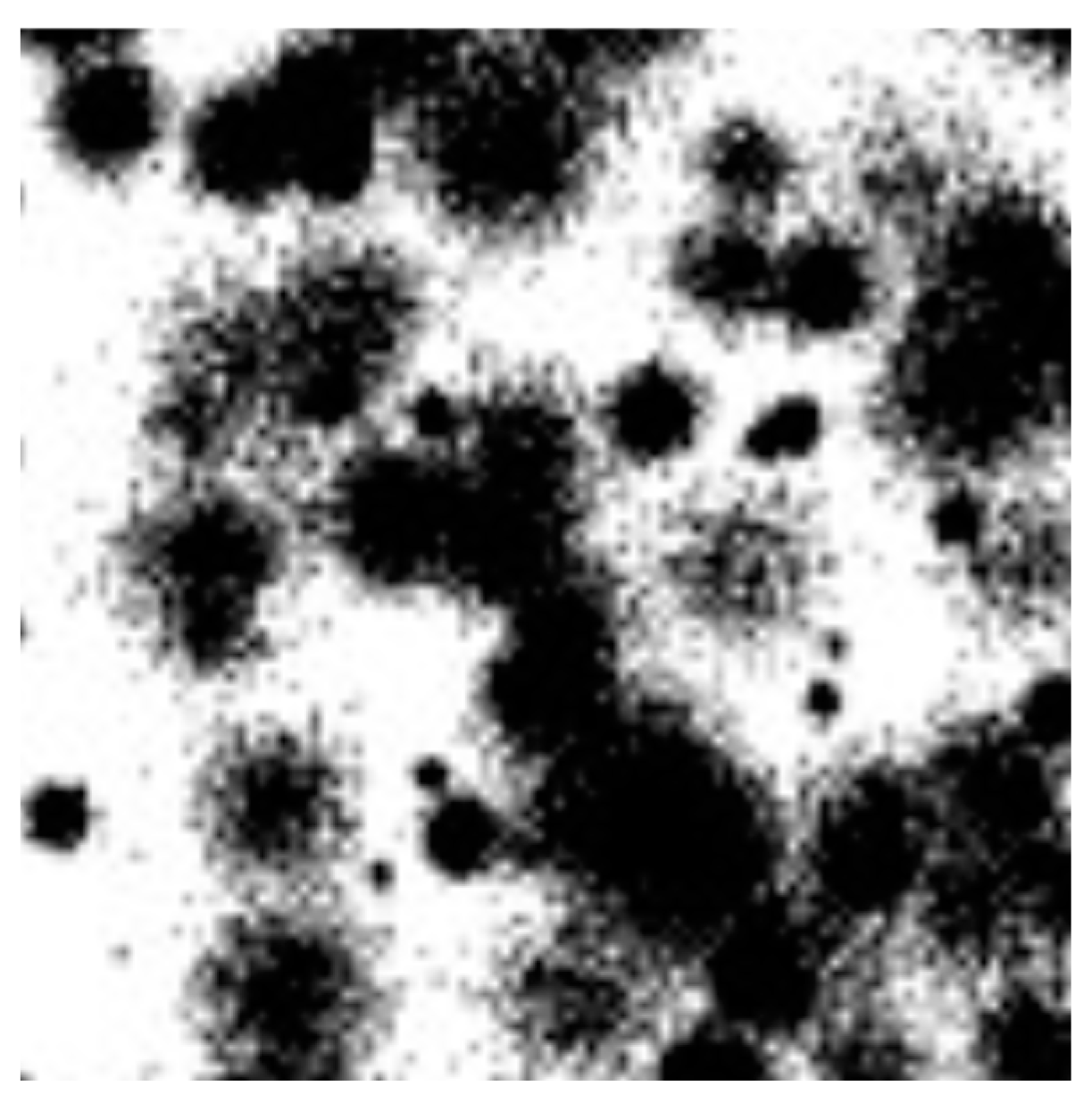
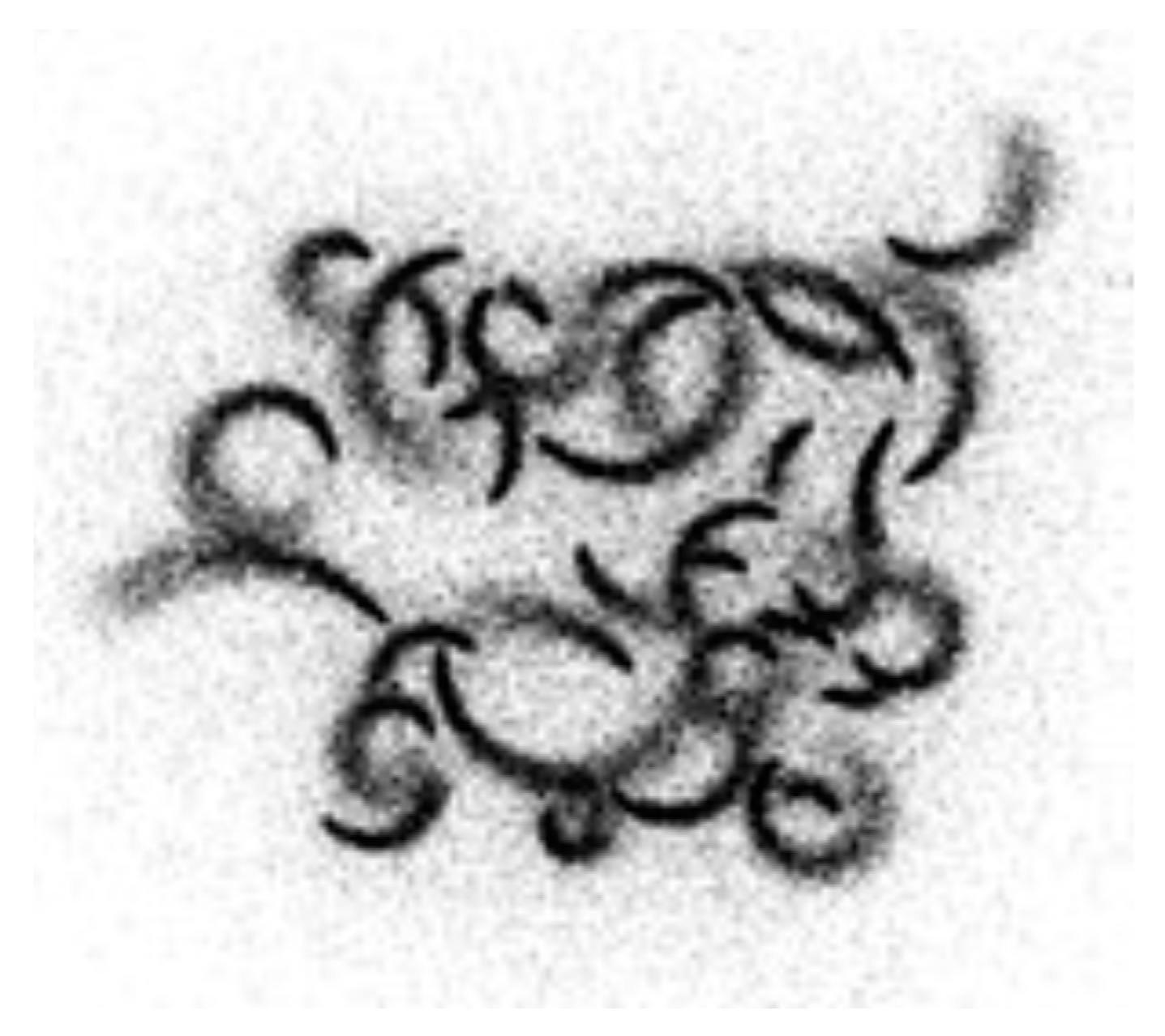
$\mathrm{B}\mathrm{i}\mathrm{r}\mathrm{c}\mathrm{h}3$ (see Figure 1) differs from the regular $\mathrm{B}\mathrm{i}\mathrm{r}\mathrm{c}\mathrm{h}1$ and $\mathrm{B}\mathrm{i}\mathrm{r}\mathrm{c}\mathrm{h}2$ because it admits clusters with a random size and randomly located in the data space. $\mathrm{W}\mathrm{o}\mathrm{r}\mathrm{m}\mathrm{s}\_2\mathrm{d}$ (see Figure 2) is composed of 35 clusters with 2-dimensional data points. $\mathrm{W}\mathrm{o}\mathrm{r}\mathrm{m}\mathrm{s}\_64\mathrm{d}$ is characterized by 25 clusters with data points with 64 dimensions. The geometrical shapes of the worm datasets are determined by starting at a random position and moving in a random direction. At any moment, the points follow a Gaussian distribution, whereby the variance gradually increases step-by-step. In addition, movement direction is continually changed according to an orthogonal direction. In $\mathrm{W}\mathrm{o}\mathrm{r}\mathrm{m}\mathrm{s}\_64\mathrm{d}$, though, the orthogonal direction gets randomly re-defined at every step.

Figure 1. The $\mathrm{B}\mathrm{i}\mathrm{r}\mathrm{c}\mathrm{h}3$ dataset [24].

Figure 2. The $\mathrm{W}\mathrm{o}\mathrm{r}\mathrm{m}\mathrm{s}\_2\mathrm{d}$ dataset [24].

Clustering of worm datasets was investigated in [26] using an enhanced and careful density peak-based algorithm [27]. $\mathrm{B}\mathrm{i}\mathrm{r}\mathrm{c}\mathrm{h}3$ was analyzed, e.g., in [9,11,12]. Such previous results will be used as a reference to assess the accuracy of the clustering solutions documented in this paper. To compare with the results in [11,12], the three datasets will be processed by first scaling down the data entries by the overall maximum.

The fourth group (see Table 5) comprises some challenging real-world datasets, many of which are without ground truth information. Clustering difficulties arise from the large number of data points, $N$, the number of point features, $D$, and the number of needed clusters, $K$.

Table 5. The fourth group of real-world datasets.

$\mathbf{D}\mathbf{a}\mathbf{t}\mathbf{a}\mathbf{s}\mathbf{e}\mathbf{t}$	$\mathbf{N}$	$\mathbf{D}$	$\mathbf{K}$
$Bridge$	$4096$	$16$	$256$
$House$	34,112	$3$	$256$
$Miss America$	$6480$	$16$	$256$
$Olivetti$	$400$	$4096$	$40$
$UrbanGB$	360,177	$2$	$469$

The non-binarized version of the $\mathrm{B}\mathrm{r}\mathrm{i}\mathrm{d}\mathrm{g}\mathrm{e}$ dataset, the 8 bits per color version of the $\mathrm{H}\mathrm{o}\mathrm{u}\mathrm{s}\mathrm{e}$ dataset, and the frame 1 vs. 2 version of $\mathrm{M}\mathrm{i}\mathrm{s}\mathrm{s} \mathrm{A}\mathrm{m}\mathrm{e}\mathrm{r}\mathrm{i}\mathrm{c}\mathrm{a}$ dataset, were downloaded from the [24] repository. They all refer to image data processing.

The image facial recognition problem of the $\mathrm{O}\mathrm{l}\mathrm{i}\mathrm{v}\mathrm{e}\mathrm{t}\mathrm{t}\mathrm{i}$ dataset, from the AT&T Laboratories Cambridge, handles $40$ human subjects, each portrayed in $10$ different poses. Every facial photo is stored by $64\times 64=4096$ pixels.

The $\mathrm{U}\mathrm{r}\mathrm{b}\mathrm{a}\mathrm{n}\mathrm{G}\mathrm{B}$ is a large dataset consisting of geographical coordinates of car accidents in Great Britain’s urban areas. The dataset can be downloaded from [28].

The solutions for the $\mathrm{O}\mathrm{l}\mathrm{i}\mathrm{v}\mathrm{e}\mathrm{t}\mathrm{t}\mathrm{i}$ and $\mathrm{U}\mathrm{r}\mathrm{b}\mathrm{a}\mathrm{n}\mathrm{G}\mathrm{B}$ reported in [11,12] were used to infer “ground truth” information about the datasets. In all the cases, though, the $SSE$ cost and its evolution vs. the real time can be used for comparison purposes.

As in [11,12], the datasets of the fourth group are processed without scaling, except for the $UrbanGB$ where the first dimension of the data entries are scaled down by a factor of $1.7$.

The following simulation experiments were executed on a Win11 Pro platform, Dell XPS 8940, Intel i7-10700 (8 physical cores), CPU@2.90 GHz, 32GB RAM and Java 17.

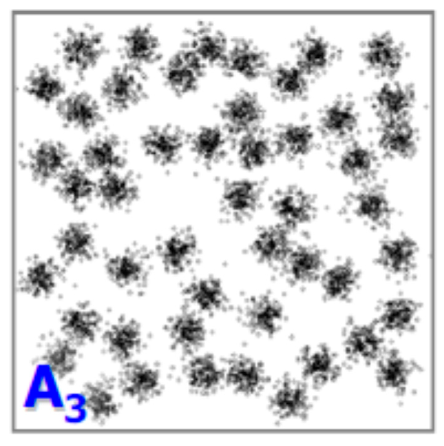
5.1. Clustering the A3 Dataset

For a preliminary study, the $A3$ dataset was chosen (see Table 2 and Figure 3). The goal was to compare the performance of classical Repeated K-Means driven by different seeding methods, to that it was achievable with PB-KM. In particular, $A3$ was first clustered via Repeated K-Means $\left(\mathrm{R}\mathrm{K}\mathrm{M}\right)$ separately fed by uniform random $\left({\mathrm{R}\mathrm{K}\mathrm{M}}^{\mathrm{U}\mathrm{n}\mathrm{i}\mathrm{f}}\right),$ K-Means++ (RKM^KM++) and Greedy K-Means++ $\left({\mathrm{R}\mathrm{K}\mathrm{M}}^{\mathrm{G}\mathrm{K}\mathrm{M}++}\right)$ seeding procedure.

Figure 3. The $\mathrm{A}3$ synthetic dataset [24].

Then, 10⁴ repetitions of K-Means were executed and the following quantities monitored: (a) the minimal value of the $\mathrm{S}\mathrm{S}\mathrm{E}$ cost $\left({\mathrm{S}\mathrm{S}\mathrm{E}}_{\mathrm{m}\mathrm{i}\mathrm{n}}\right),$ (b) the corresponding Cluster Index $\left(\mathrm{C}\mathrm{I}\right)$ value (see Section 2.5) (${\mathrm{C}\mathrm{I}}_{\mathrm{m}\mathrm{i}\mathrm{n} \left(\mathrm{S}\mathrm{S}\mathrm{E}\right)}$), (c) the minimal value of the observed $\mathrm{C}\mathrm{I}$ (${\mathrm{C}\mathrm{I}}_{\mathrm{m}\mathrm{i}\mathrm{n}}$) and the corresponding value of the $\mathrm{S}\mathrm{S}\mathrm{E}$ cost (${\mathrm{S}\mathrm{S}\mathrm{E}}_{\mathrm{m}\mathrm{i}\mathrm{n}\left(\mathrm{C}\mathrm{I}\right)}$), (d) the emerging average $\mathrm{C}\mathrm{I}$ value ($\mathrm{a}\mathrm{v}\mathrm{g}\_\mathrm{C}\mathrm{I}$) and (e) the $\mathrm{s}\mathrm{u}\mathrm{c}\mathrm{c}\mathrm{e}\mathrm{s}\mathrm{s}\_\mathrm{r}\mathrm{a}\mathrm{t}\mathrm{e}$, that is, the number of runs which ended with a $\mathrm{C}\mathrm{I}=0$, divided by 10⁴. In addition, the Parallel Execution Time ($\mathrm{P}\mathrm{E}\mathrm{T}$), in sec, needed by Repeated K-Means to complete its runs was also observed. Table 6 collects all the achieved results.

Table 6. Clustering experimental results on the $\mathrm{A}3$ dataset.

	${\mathbf{R}\mathbf{K}\mathbf{M}}^{\mathbf{U}\mathbf{n}\mathbf{i}\mathbf{f}}$	${\mathbf{R}\mathbf{K}\mathbf{M}}^{\mathbf{K}\mathbf{M}++}$	${\mathbf{R}\mathbf{K}\mathbf{M}}^{\mathbf{G}\mathbf{K}\mathbf{M}++}$
${\mathrm{S}\mathrm{S}\mathrm{E}}_{\mathrm{m}\mathrm{i}\mathrm{n}}$	$7.44$	$6.74$	$6.74$
${\mathrm{C}\mathrm{I}}_{\mathrm{m}\mathrm{i}\mathrm{n} \left(\mathrm{S}\mathrm{S}\mathrm{E}\right)}$	$1$	$0$	$0$
${\mathrm{C}\mathrm{I}}_{\mathrm{m}\mathrm{i}\mathrm{n}}$	$1$	$0$	$0$
${\mathrm{S}\mathrm{S}\mathrm{E}}_{\mathrm{m}\mathrm{i}\mathrm{n} \left(\mathrm{C}\mathrm{I}\right)}$	$7.44$	$6.74$	$6.74$
$\mathrm{a}\mathrm{v}\mathrm{g}\_\mathrm{C}\mathrm{I}$	$6.58$	$4.17$	$1.62$
$\mathrm{s}\mathrm{u}\mathrm{c}\mathrm{c}\mathrm{e}\mathrm{s}\mathrm{s}\_\mathrm{r}\mathrm{a}\mathrm{t}\mathrm{e}$	$0\mathrm{\%}$	$0.01\mathrm{\%}$	$5.8\mathrm{\%}$
$\mathrm{P}\mathrm{E}\mathrm{T}\left(\mathrm{s}\right)$	$103$	$154$	$990$

The experimental data in Table 6 clearly confirm the superior behavior ensured by GKM++ seeding, which makes $\mathrm{R}\mathrm{K}\mathrm{M}$ capable of outperforming the scenarios where K-Means++ (KM++) or the uniform random (Unif) centroids initialization is adopted. The observed average $\mathrm{C}\mathrm{I}$ and the $\mathrm{s}\mathrm{u}\mathrm{c}\mathrm{c}\mathrm{e}\mathrm{s}\mathrm{s} \mathrm{r}\mathrm{a}\mathrm{t}\mathrm{e}$ are worth being noted. As one case see in Table 6, it always happens that the minimum $\mathrm{C}\mathrm{I}$ value occurs at the minimum $\mathrm{S}\mathrm{S}\mathrm{E}$ cost.

The ${\mathrm{R}\mathrm{K}\mathrm{M}}^{\mathrm{G}\mathrm{K}\mathrm{M}++}$ results in Table 6 comply with the results reported, e.g., in [9,11].

Table 7 collects the results observed when using PB-KM with the parameter values $\mathrm{J}=25$ and ${\mathrm{R}}_1=3$ adopted in the first step (see Algorithm 4), and the value ${\mathrm{R}}_2=40$ used for the second step. Only the $\mathrm{P}\mathrm{E}\mathrm{T}$ was annotated for the first step, which creates the population of candidate solutions. The second-step results clearly confirm that PB-KM is able to correctly solve the $\mathrm{A}3$ dataset. In fact, a $\mathrm{s}\mathrm{u}\mathrm{c}\mathrm{c}\mathrm{e}\mathrm{s}\mathrm{s}\_\mathrm{r}\mathrm{a}\mathrm{t}\mathrm{e}$ of 100% and $\mathrm{C}\mathrm{I}=0$ were observed. The $\mathrm{S}\mathrm{S}\mathrm{E}$ minimal value coincides with that obtained with ${\mathrm{R}\mathrm{K}\mathrm{M}}^{\mathrm{G}\mathrm{K}\mathrm{M}++}$ in Table 6.

Table 7. PB-KM experimental results about the $A3$ dataset.

	$\mathbf{P}\mathbf{B}-\mathbf{K}\mathbf{M}$$(\mathbf{J}=25, {\mathbf{R}}_1=3), {\mathbf{R}}_2=40$
${\mathrm{P}\mathrm{E}\mathrm{T}}_1\left(\mathrm{s}\right)$	$6.4$
${\mathrm{S}\mathrm{S}\mathrm{E}}_{\mathrm{m}\mathrm{i}\mathrm{n}}$	$6.74$
${\mathrm{C}\mathrm{I}}_{\mathrm{m}\mathrm{i}\mathrm{n} \left(\mathrm{S}\mathrm{S}\mathrm{E}\right)}$	$0$
${\mathrm{C}\mathrm{I}}_{\mathrm{m}\mathrm{i}\mathrm{n}}$	$0$
${\mathrm{S}\mathrm{S}\mathrm{E}}_{\mathrm{m}\mathrm{i}\mathrm{n} \left(\mathrm{C}\mathrm{I}\right)}$	$6.74$
$\mathrm{a}\mathrm{v}\mathrm{g}\_\mathrm{C}\mathrm{I}$	$0$
$\mathrm{s}\mathrm{u}\mathrm{c}\mathrm{c}\mathrm{e}\mathrm{s}\mathrm{s}\_\mathrm{r}\mathrm{a}\mathrm{t}\mathrm{e}$	$100\%$
${\mathrm{P}\mathrm{E}\mathrm{T}}_2\left(\mathrm{s}\right)$	$2.4$

Results in Table 7 also show how the execution time of PB-KM outperforms that achievable by straight Repeated K-Means (see Table 6). The same results of minimal $SSE$ and $\mathrm{C}\mathrm{I},$ and a 100% $\mathrm{s}\mathrm{u}\mathrm{c}\mathrm{c}\mathrm{e}\mathrm{s}\mathrm{s}\_\mathrm{r}\mathrm{a}\mathrm{t}\mathrm{e}$ were also observed when using ${\mathrm{R}}_2=10$. In reality, one single recombination iteration is sufficient for obtaining the minimal $\mathrm{S}\mathrm{S}\mathrm{E}$ and $\mathrm{C}\mathrm{I}$. All of this was precisely confirmed by using the PB-RS recombination on the same population created by PB-KM.

The following sections report the experimental results collected by applying PB-KM/PB-RS to the four groups of selected datasets. A common point of all the experiments concerns using the GKM++ seeding method both in the first step of the population set-up and in the second step of recombination.

5.2. First Group of Synthetic Datasets (Table 2)

Table 8 shows the experimental results collected when applying PB-KM to all the benchmark datasets reported in Table 2 (entries are preliminary scaled down by the overall maximum). It is worth noting that all these datasets have a $\mathrm{s}\mathrm{u}\mathrm{c}\mathrm{c}\mathrm{e}\mathrm{s}\mathrm{s}\_\mathrm{r}\mathrm{a}\mathrm{t}\mathrm{e}$ of $0\%$ when clustered by Repeated K-Means together with uniform random seeding, as also documented in [5]. The experimental results confirm that $\mathrm{C}\mathrm{I}=0$ always occurs at the minimum value of the objective $\mathrm{S}\mathrm{S}\mathrm{E}$ cost.

Table 8. PB-KM results on the synthetic datasets of Table 2.

$\mathbf{D}\mathbf{a}\mathbf{t}\mathbf{a}\mathbf{s}\mathbf{e}\mathbf{t}$	$\mathbf{m}\mathbf{i}\mathbf{n} \left(\mathbf{S}\mathbf{S}\mathbf{E}\right)$	${\mathbf{C}\mathbf{I}}_{\mathbf{m}\mathbf{i}\mathbf{n} \left(\mathbf{S}\mathbf{S}\mathbf{E}\right)}$	$\mathbf{a}\mathbf{v}\mathbf{g}\_\mathbf{C}\mathbf{I}$	$\mathbf{S}\mathbf{u}\mathbf{c}\mathbf{c}\mathbf{e}\mathbf{s}\mathbf{s}\_\mathbf{R}\mathbf{a}\mathbf{t}\mathbf{e}$	${\mathbf{P}\mathbf{E}\mathbf{T}}_1\left(\mathbf{s}\right)$	${\mathbf{P}\mathbf{E}\mathbf{T}}_2\left(\mathbf{s}\right)$
$A3$	6.74	0	0	100%	6.4	2.4
$S3$	18.82	0	0	100%	1.1	0.5
$Dim1024$	5.39	0	0	100%	9.4	4.0
$Unbalance$	0.65	0	0	100%	0.6	0.3
$Birch1$	92.77	0	0	100%	277.3	96.6
$Birch2$	0.46	0	0	100%	242.2	99.0

The $\mathrm{S}3$, $\mathrm{D}\mathrm{i}\mathrm{m}1024$ and $\mathrm{U}\mathrm{n}\mathrm{b}\mathrm{a}\mathrm{l}\mathrm{a}\mathrm{n}\mathrm{c}\mathrm{e}$ datasets were studied using $\mathrm{J}=25$ and ${\mathrm{R}}_1=3$ for the first step (three independent repetitions of K-Means are used for defining each solution of the population), and by ${\mathrm{R}}_2=40$ for the second step (see Algorithm 4). Due to the higher number of clusters $K$, $\mathrm{B}\mathrm{i}\mathrm{r}\mathrm{c}\mathrm{h}1$ and $\mathrm{B}\mathrm{i}\mathrm{r}\mathrm{c}\mathrm{h}2$ were instead studied by using $\mathrm{J}=20$ and ${\mathrm{R}}_1=3$ for the first step, and ${\mathrm{R}}_2=40$ for the second step. Table 8 reports the Parallel Elapsed Time ($\mathrm{P}\mathrm{E}\mathrm{T}$) in sec, required by the first and second step of PB-KM.

In reality, PB-KM was capable of detecting the “best” solution, that is, one with a minimal $\mathrm{S}\mathrm{S}\mathrm{E}$ and $\mathrm{C}\mathrm{I}$, just after a few iterations (in some cases after 1 iteration) of the recombination step. All of this was also confirmed by PB-RS recombination. The results (e.g., CI = 0) in Table 8 are the same as reported in [9], where Random Swap was used, and in [11] where the Recombinator-K-Means tool was exploited.

5.3. Second Group of Real-World Datasets (Table 3)

The $\mathrm{M}\mathrm{u}\mathrm{s}\mathrm{k}$ and $\mathrm{M}\mathrm{i}\mathrm{n}\mathrm{i}\mathrm{B}\mathrm{o}\mathrm{o}\mathrm{N}\mathrm{E}$ real-world datasets (data entries preliminarily scaled by min-max normalization), together with the ground truth information inferred from the solutions reported in [14], were easily clustered using PB-KM with $\mathrm{J}=25$ and ${\mathrm{R}}_1=3$ for the first step, and ${\mathrm{R}}_2=20$ for the second step. The results, which coincide with those reported in [11,12,14], are shown in Table 9. Very few iterations of PB-RS also confirmed them.

Table 9. PB-KM results on the real-world datasets of Table 3.

$\mathbf{D}\mathbf{a}\mathbf{t}\mathbf{a}\mathbf{s}\mathbf{e}\mathbf{t}$	$\mathbf{m}\mathbf{i}\mathbf{n} \left(\mathbf{S}\mathbf{S}\mathbf{E}\right)$	${\mathbf{C}\mathbf{I}}_{\mathbf{m}\mathbf{i}\mathbf{n} \left(\mathbf{S}\mathbf{S}\mathbf{E}\right)}$	$\mathbf{a}\mathbf{v}\mathbf{g}\_\mathbf{C}\mathbf{I}$	$\mathbf{S}\mathbf{u}\mathbf{c}\mathbf{c}\mathbf{e}\mathbf{s}\mathbf{s}\_\mathbf{R}\mathbf{a}\mathbf{t}\mathbf{e}$	${\mathbf{P}\mathbf{E}\mathbf{T}}_1\left(\mathbf{s}\right)$	${\mathbf{P}\mathbf{E}\mathbf{T}}_2\left(\mathbf{s}\right)$
$Musk$	36,373	0	0	100%	0.5	0.1
$MiniBooNE$	2802	0	0	100%	5.3	0.8

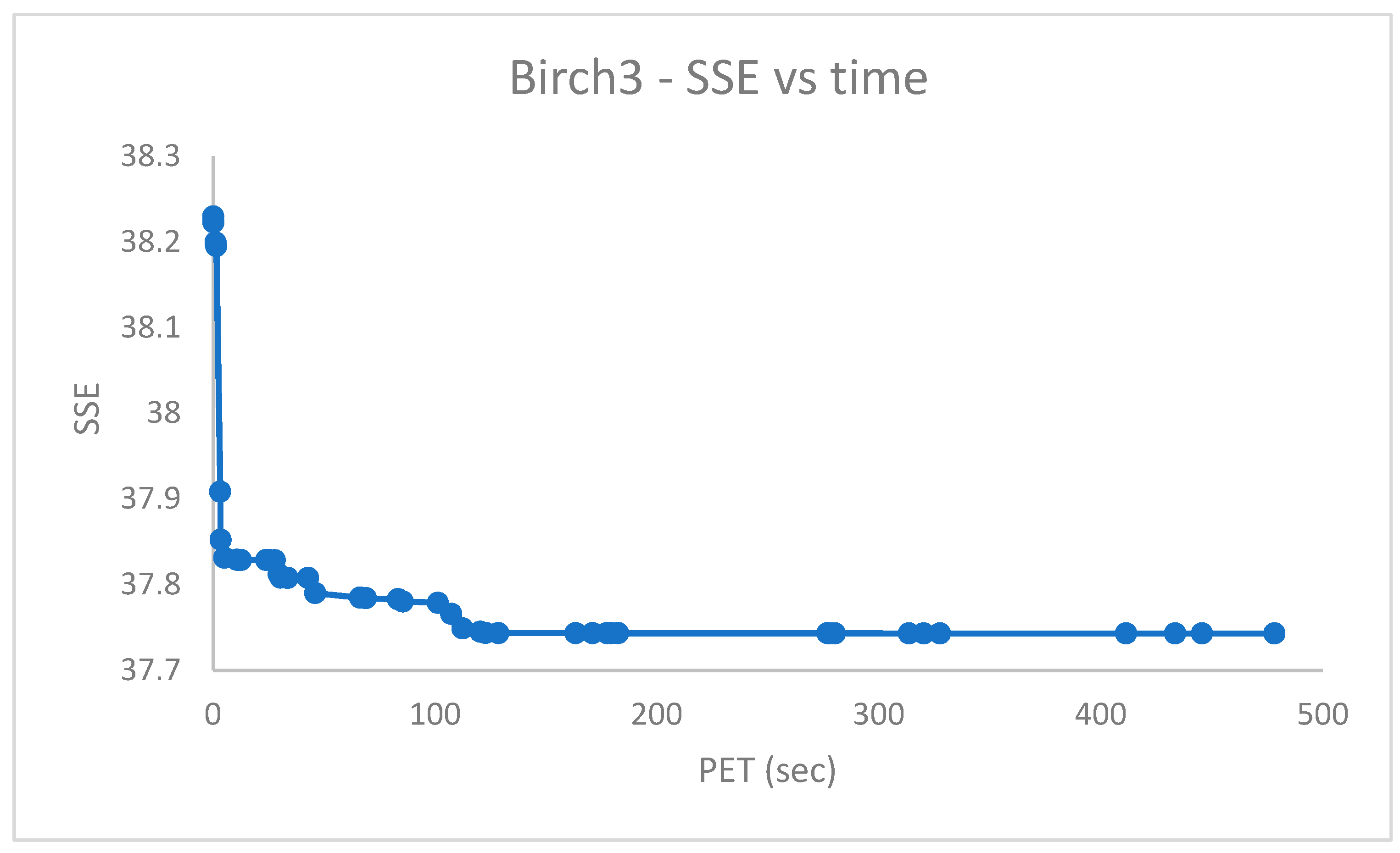
5.4. Third Group of Synthetic Datasets (Table 4)

All the entries of datasets in Table 4 were preliminarily scaled by the overall maximum. The datasets of this group were processed via PB-RS because it provided the most accurate results. The initial population of $\mathrm{B}\mathrm{i}\mathrm{r}\mathrm{c}\mathrm{h}3$ was built using $J=20$ and $T=5000$ swap iterations of Random Swap always seeded by GKM++, requiring a parallel elapsed time of $\mathrm{P}\mathrm{E}\mathrm{T}=5041$ s. The recombination step was carried out using $T=$ 10,000 iterations. Figure 4 depicts the $\mathrm{S}\mathrm{S}\mathrm{E}$ vs. the real-time PET (s). 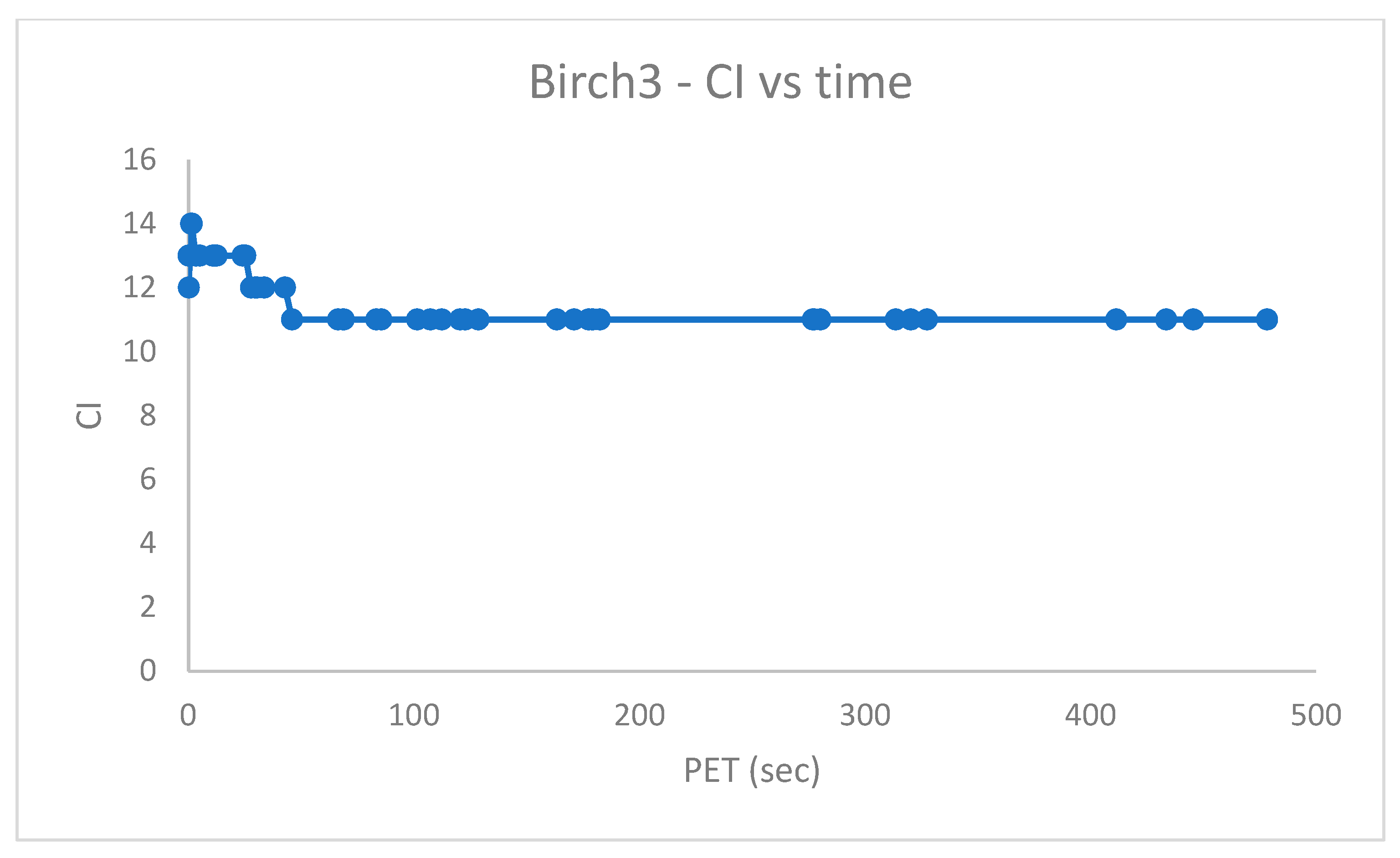Figure 5 shows the Cluster Index (recall $\mathrm{B}\mathrm{i}\mathrm{r}\mathrm{c}\mathrm{h}3$ comes with ground truth centroids, see also Section 2.5) $\mathrm{C}\mathrm{I}$ vs. real-time PET (s).

Figure 4. $\mathrm{S}\mathrm{S}\mathrm{E}$ cost vs. time for the $\mathrm{B}\mathrm{i}\mathrm{r}\mathrm{c}\mathrm{h}3$ dataset.

Figure 5. $\mathrm{C}\mathrm{e}\mathrm{n}\mathrm{t}\mathrm{r}\mathrm{o}\mathrm{i}\mathrm{d} \mathrm{I}\mathrm{n}\mathrm{d}\mathrm{e}\mathrm{x} \left(\mathrm{C}\mathrm{I}\right)$ vs. time for the $\mathrm{B}\mathrm{i}\mathrm{r}\mathrm{c}\mathrm{h}3$ dataset.

Notably, a $\mathrm{C}\mathrm{I}=12$ was estimated in [9] by using standard Parallel Random Swap executed for ${10}^5$ iterations, requiring a $\mathrm{P}\mathrm{E}\mathrm{T}=7341 \mathrm{s}\mathrm{e}\mathrm{c}$. Figure 5 suggests a final value of $\mathrm{C}\mathrm{I}=11$, after a significantly smaller time.

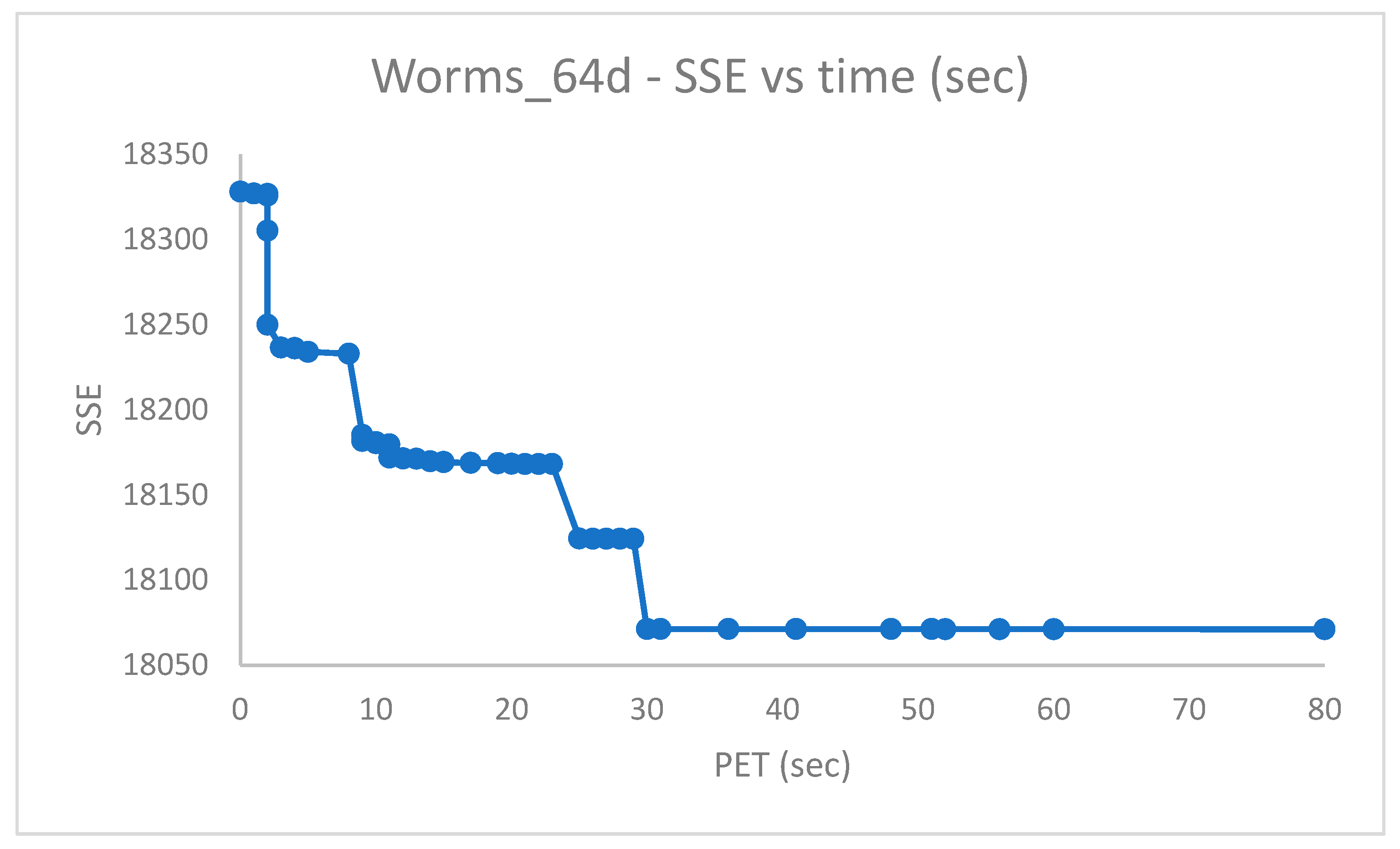
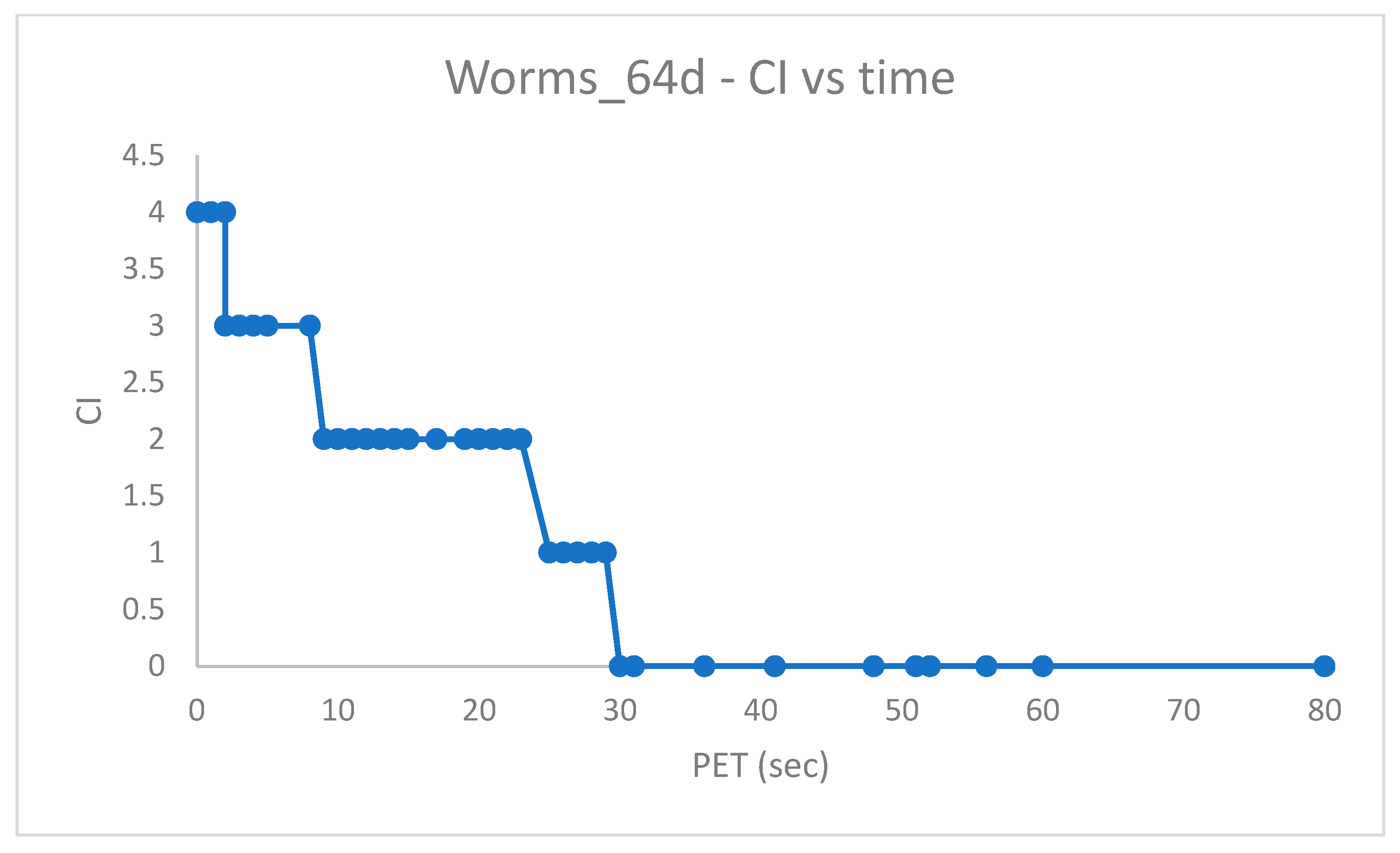
To ensure a proper number of candidate centroids for the $\mathrm{W}\mathrm{o}\mathrm{r}\mathrm{m}\mathrm{s}\_2\mathrm{d}/\mathrm{W}\mathrm{o}\mathrm{r}\mathrm{m}\mathrm{s}\_64\mathrm{d}$ datasets which have $K=35$ and $K=25$ clusters, respectively, a population with $J=40$ solutions and $\mathrm{T}=5000$ swap iterations was preliminarily created with PB-RS, requiring $\mathrm{P}\mathrm{E}\mathrm{T}=4485$ sec for $\mathrm{W}\mathrm{o}\mathrm{r}\mathrm{m}\mathrm{s}\_2\mathrm{d}$, and a population of $\mathrm{J}=40$ solutions and ${\mathrm{R}}_1=3$ with PB-KM, requiring $\mathrm{P}\mathrm{E}\mathrm{T}=5156 \mathrm{s}\mathrm{e}\mathrm{c}$ for $\mathrm{W}\mathrm{o}\mathrm{r}\mathrm{m}\mathrm{s}\_64$.

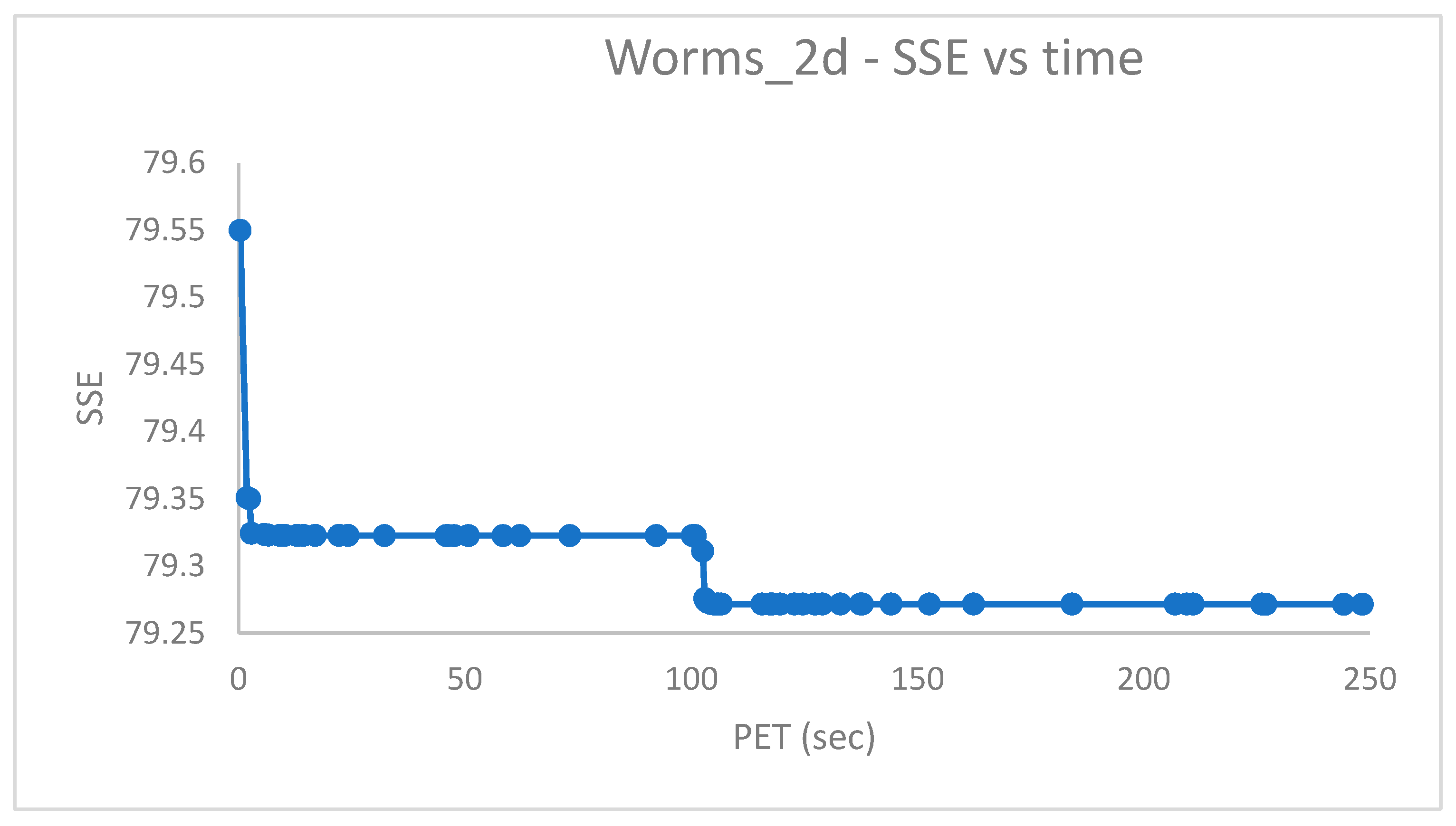
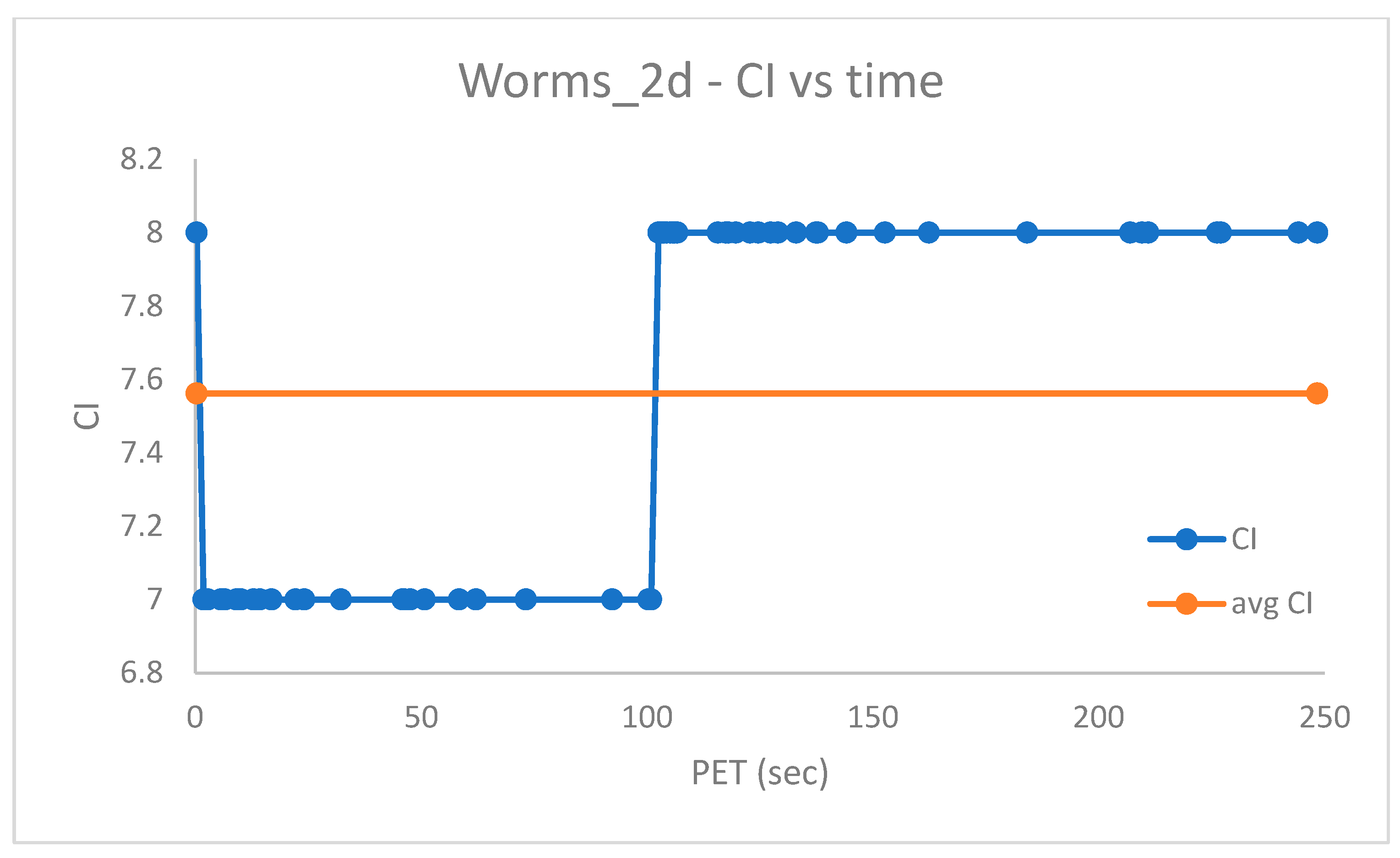
The PB-RS recombination step lasts after $T={10}^4$ iterations for $\mathrm{W}\mathrm{o}\mathrm{r}\mathrm{m}\mathrm{s}\_2\mathrm{d}$. Figure 6 and Figure 7 show the measured $\mathrm{S}\mathrm{S}\mathrm{E}$ vs. time and the $\mathrm{C}\mathrm{I}$ vs. time for $\mathrm{W}\mathrm{o}\mathrm{r}\mathrm{m}\mathrm{s}\_2\mathrm{d}$, respectively. Since the worm datasets come with partition labels as ground truth, the $\mathrm{C}\mathrm{I}$ is, in reality, a Generalized $\mathrm{C}\mathrm{I}$ [23] based on the Jaccard distance among the partitions (see also [9])).

Figure 6. $\mathrm{S}\mathrm{S}\mathrm{E}$ cost vs. time for the $\mathrm{W}\mathrm{o}\mathrm{r}\mathrm{m}\mathrm{s}\_2\mathrm{d}$ dataset.

Figure 7. $\left(\mathrm{G}\mathrm{e}\mathrm{n}\mathrm{e}\mathrm{r}\mathrm{a}\mathrm{l}\mathrm{i}\mathrm{z}\mathrm{e}\mathrm{d}\right) \mathrm{C}\mathrm{e}\mathrm{n}\mathrm{t}\mathrm{r}\mathrm{o}\mathrm{i}\mathrm{d} \mathrm{I}\mathrm{n}\mathrm{d}\mathrm{e}\mathrm{x} \left(\mathrm{C}\mathrm{I}\right)$ vs. time for the $\mathrm{W}\mathrm{o}\mathrm{r}\mathrm{m}\mathrm{s}\_2\mathrm{d}$ dataset.

Figure 6 confirms that for a dataset like $\mathrm{W}\mathrm{o}\mathrm{r}\mathrm{m}\mathrm{s}\_2\mathrm{d}$, the minimization of the $\mathrm{S}\mathrm{S}\mathrm{E}$ cost does imply the most accurate solution to be achieved (here assessed according to the Cluster Index $\mathrm{C}\mathrm{I}$). In fact, for lower values of the $\mathrm{S}\mathrm{S}\mathrm{E}$ (see Figure 6), the $\mathrm{C}\mathrm{I}$ increases. The average value $\mathrm{C}\mathrm{I}=7.6$ in Figure 7 complies with a similar result documented in [26].

As discussed in [9], the $\mathrm{W}\mathrm{o}\mathrm{r}\mathrm{m}\mathrm{s}\_64\mathrm{d}$, despite the higher dimensionality w.r.t. $\mathrm{W}\mathrm{o}\mathrm{r}\mathrm{m}\mathrm{s}\_2\mathrm{d}$, is more amenable to clustering and can be correctly solved via Random Swap. This was confirmed using PB-RS with a recombination step of $\mathrm{T}=1000$ swap iterations (fewer iterations could have been used as well).

Figure 8 and Figure 9 show the $\mathrm{S}\mathrm{S}\mathrm{E}$ vs. time and the $\mathrm{C}\mathrm{I}$ vs. time for $\mathrm{W}\mathrm{o}\mathrm{r}\mathrm{m}\mathrm{s}\_64\mathrm{d}$, respectively. As shown in Figure 9, the ultimate value of $\mathrm{C}\mathrm{I}$ is 0, which starts occurring at the minimum $\mathrm{S}\mathrm{S}\mathrm{E}$ (see Figure 8), thus witnessing the obtainment of a solution with correctly structured clusters.

Figure 8. $\mathrm{S}\mathrm{S}\mathrm{E}$ cost vs. time for the $\mathrm{W}\mathrm{o}\mathrm{r}\mathrm{m}\mathrm{s}\_64\mathrm{d}$ dataset.

Figure 9. $\left(\mathrm{G}\mathrm{e}\mathrm{n}\mathrm{e}\mathrm{r}\mathrm{a}\mathrm{l}\mathrm{i}\mathrm{z}\mathrm{e}\mathrm{d}\right) \mathrm{C}\mathrm{e}\mathrm{n}\mathrm{t}\mathrm{r}\mathrm{o}\mathrm{i}\mathrm{d} \mathrm{I}\mathrm{n}\mathrm{d}\mathrm{e}\mathrm{x} \left(\mathrm{C}\mathrm{I}\right)$ vs. time for the $\mathrm{W}\mathrm{o}\mathrm{r}\mathrm{m}\mathrm{s}\_64\mathrm{d}$ dataset.

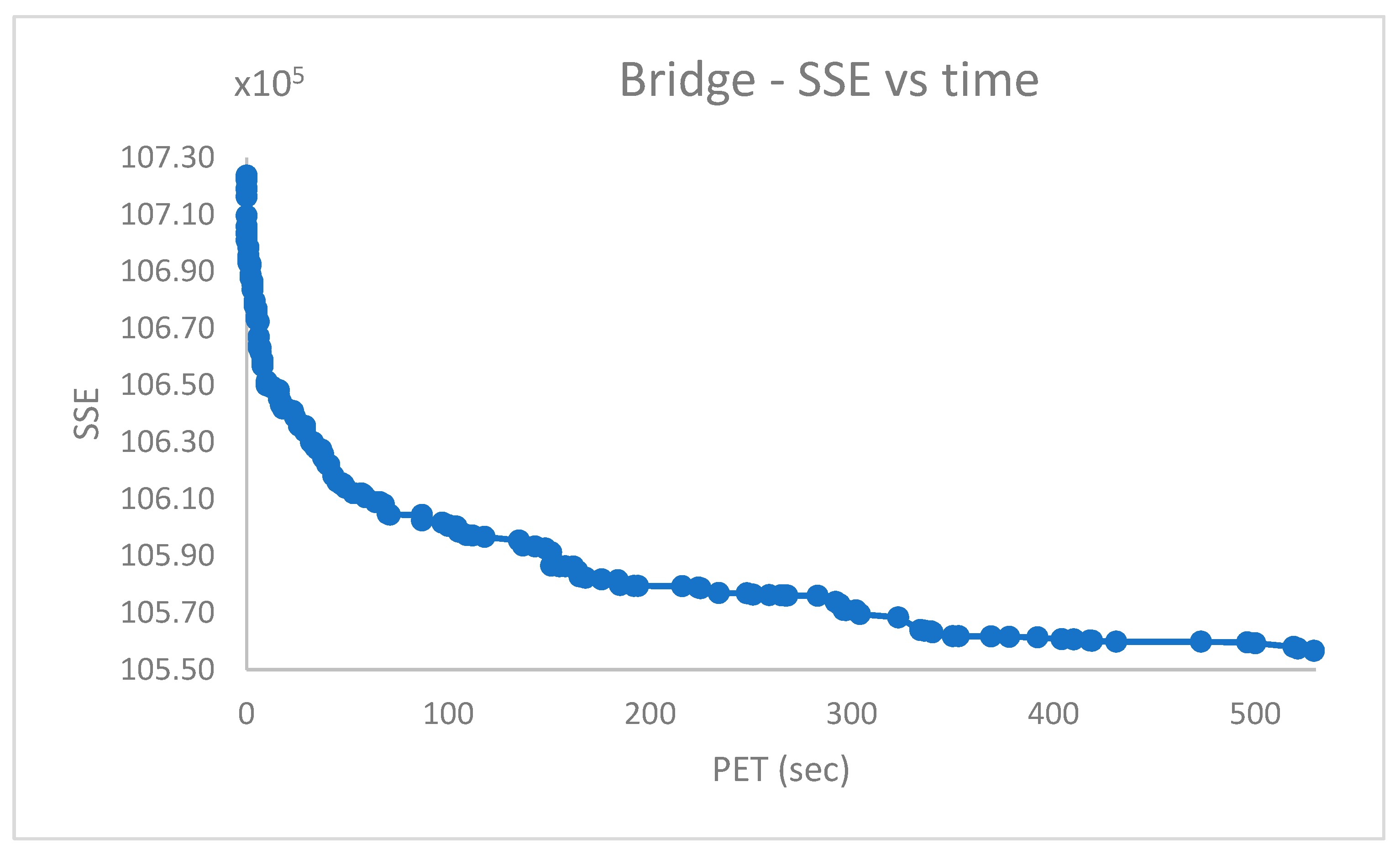
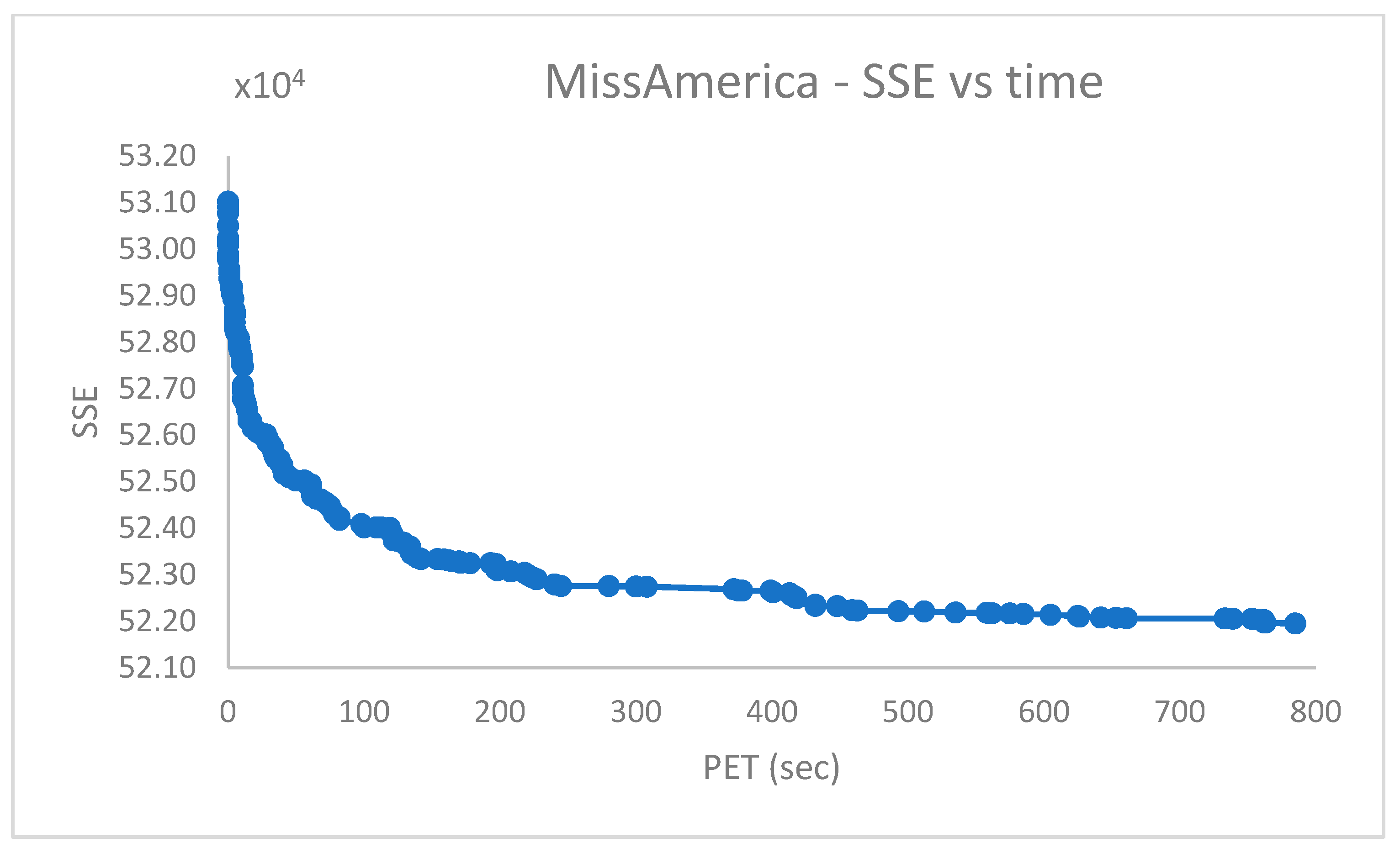
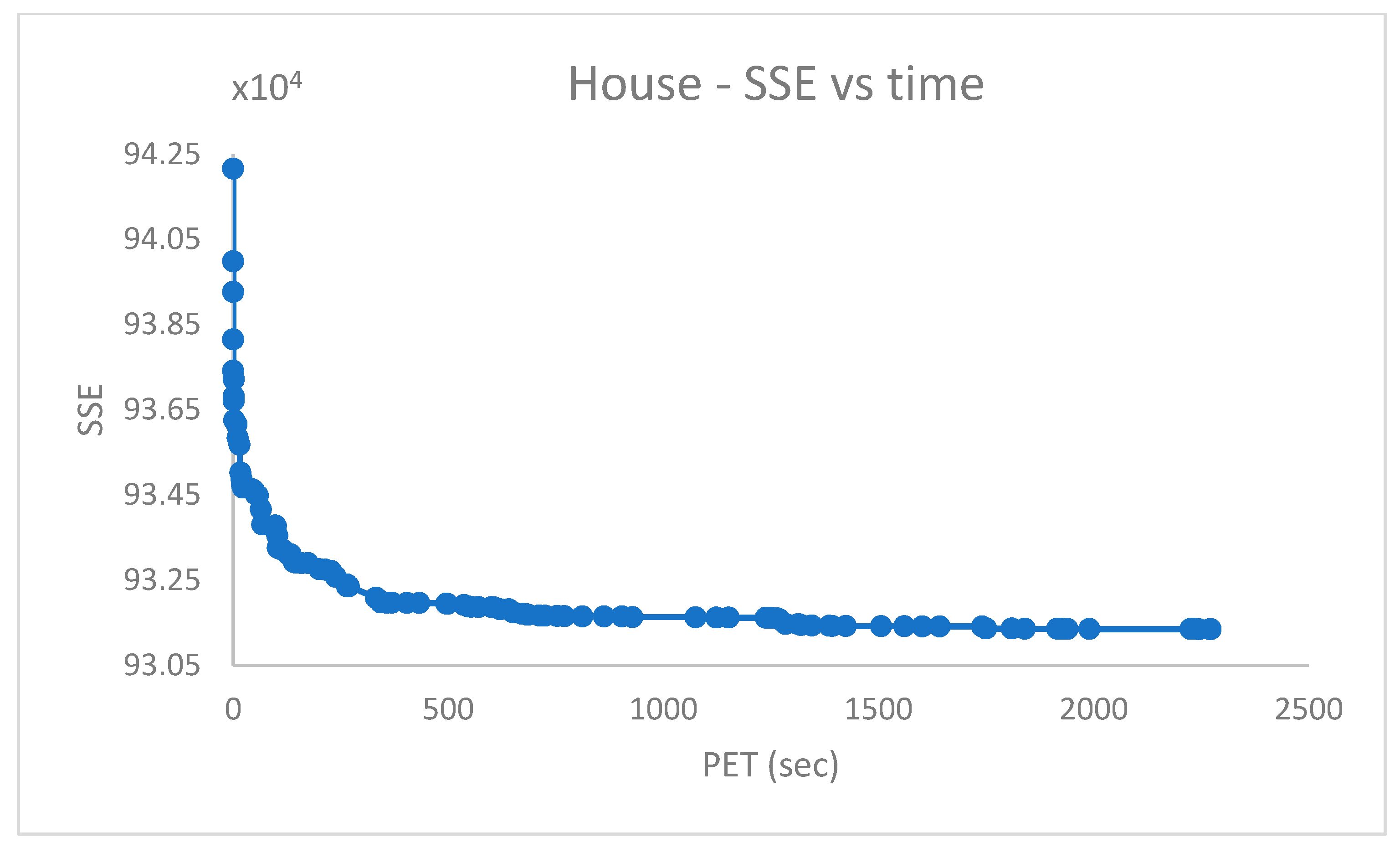
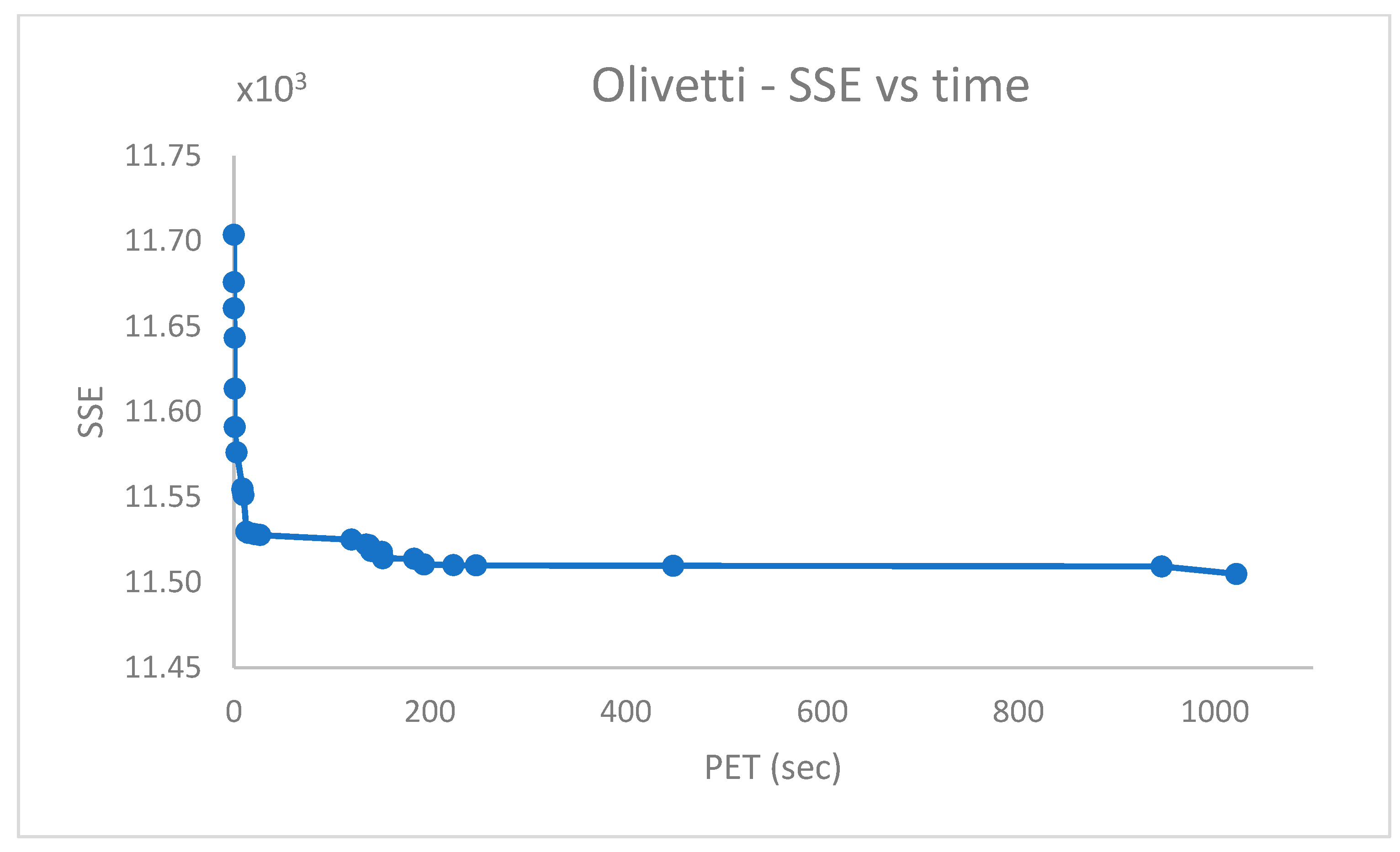
5.5. Fourth Group of Real-World Datasets (Table 5)

The challenging real-world datasets in Table 5, which have many clusters, were clustered by PB-RS by preparing a population of $J=5$ solutions each emerging after $T=5000$ iterations of Random Swap. PB-RS was chosen because it provided better experimental results (in terms of accuracy and time efficiency) w.r.t. PB-KM.

The dataset entries were used without scaling, except for the $\mathrm{U}\mathrm{r}\mathrm{b}\mathrm{a}\mathrm{n}\mathrm{G}\mathrm{B}$. In the $\mathrm{U}\mathrm{r}\mathrm{b}\mathrm{a}\mathrm{n}\mathrm{G}\mathrm{B}$, instead, the first dimension of the data entries is preliminarily scaled down by a factor of $1.7$. The recombination step lasts after $\mathrm{T}={5\times 10}^4$ iterations. However, it can be terminated when the current cost differs from the previous one of a quantity less than a given numerical threshold (e.g., ${10}^{-4}$).

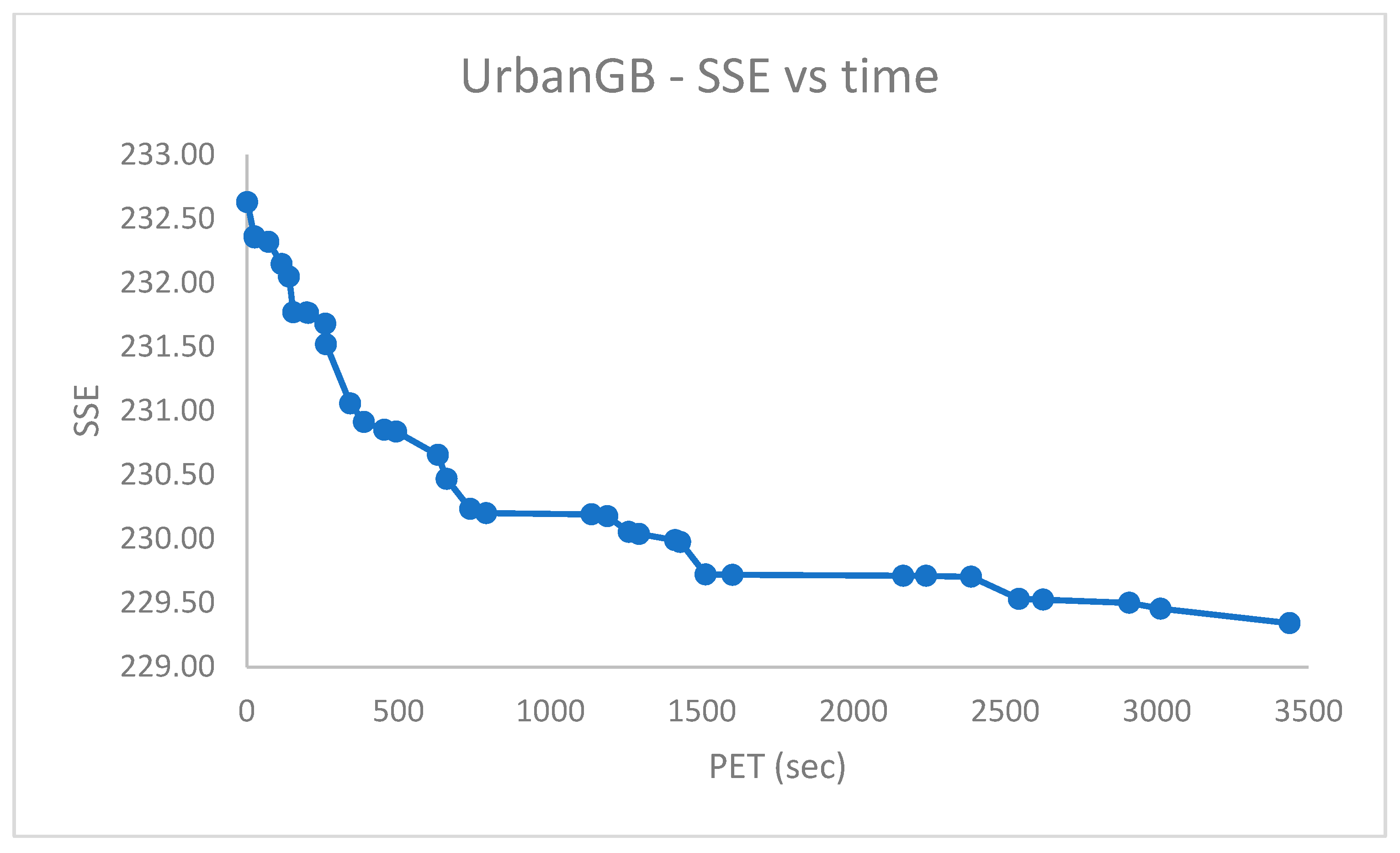
Figure 10, Figure 11, Figure 12, Figure 13, Figure 14, Figure 15 and Figure 16 report the performance curves (the $\mathrm{S}\mathrm{S}\mathrm{E}$ cost vs. time and, when possible, the $\mathrm{C}\mathrm{I}$ vs. time) observed for the $\mathrm{B}\mathrm{r}\mathrm{i}\mathrm{d}\mathrm{g}\mathrm{e}$, $\mathrm{H}\mathrm{o}\mathrm{u}\mathrm{s}\mathrm{e}$, $\mathrm{M}\mathrm{i}\mathrm{s}\mathrm{s}\mathrm{A}\mathrm{m}\mathrm{e}\mathrm{r}\mathrm{i}\mathrm{c}\mathrm{a}$, $\mathrm{O}\mathrm{l}\mathrm{i}\mathrm{v}\mathrm{e}\mathrm{t}\mathrm{t}\mathrm{i}$ and $\mathrm{U}\mathrm{r}\mathrm{b}\mathrm{a}\mathrm{n}\mathrm{G}\mathrm{B}$ [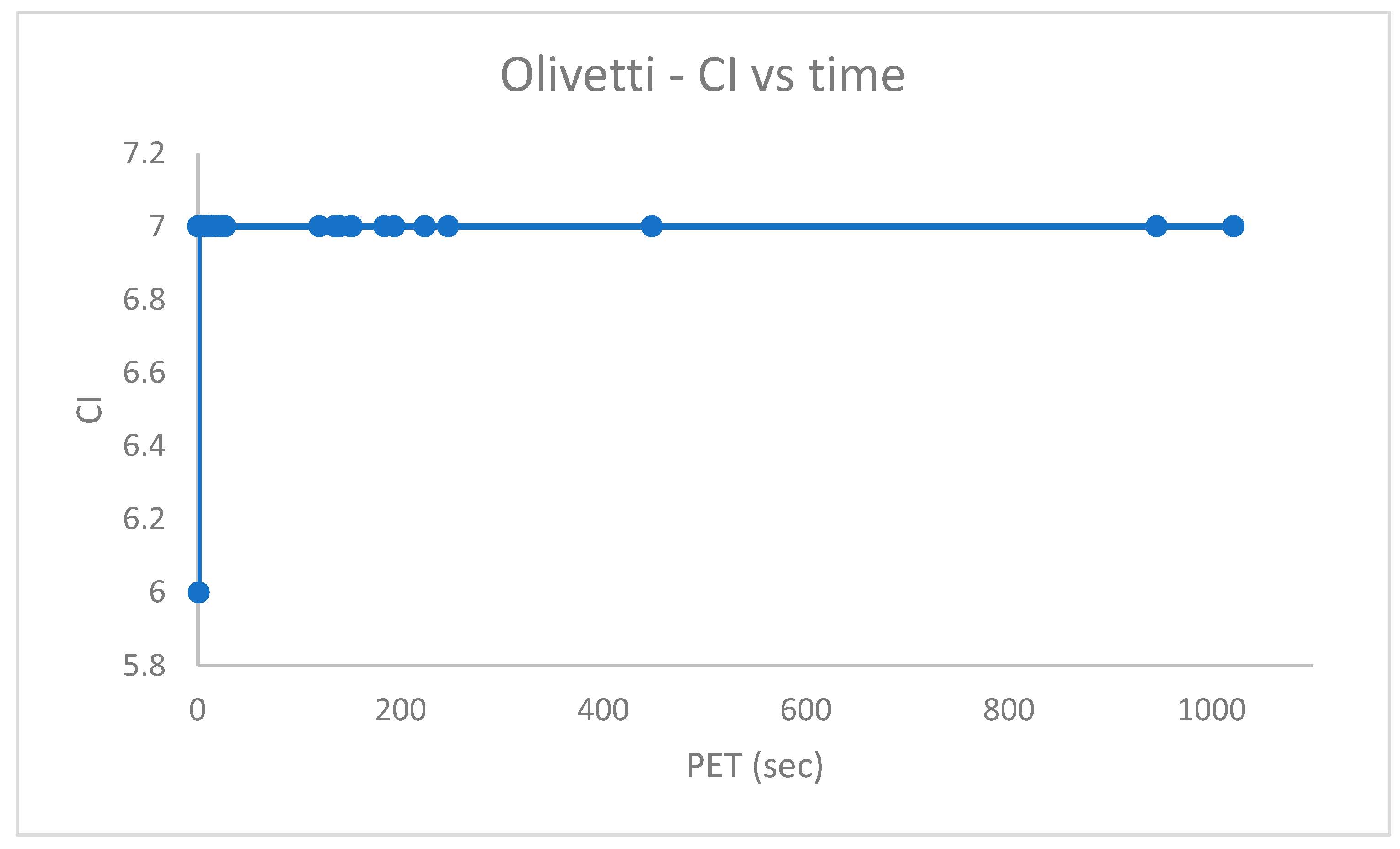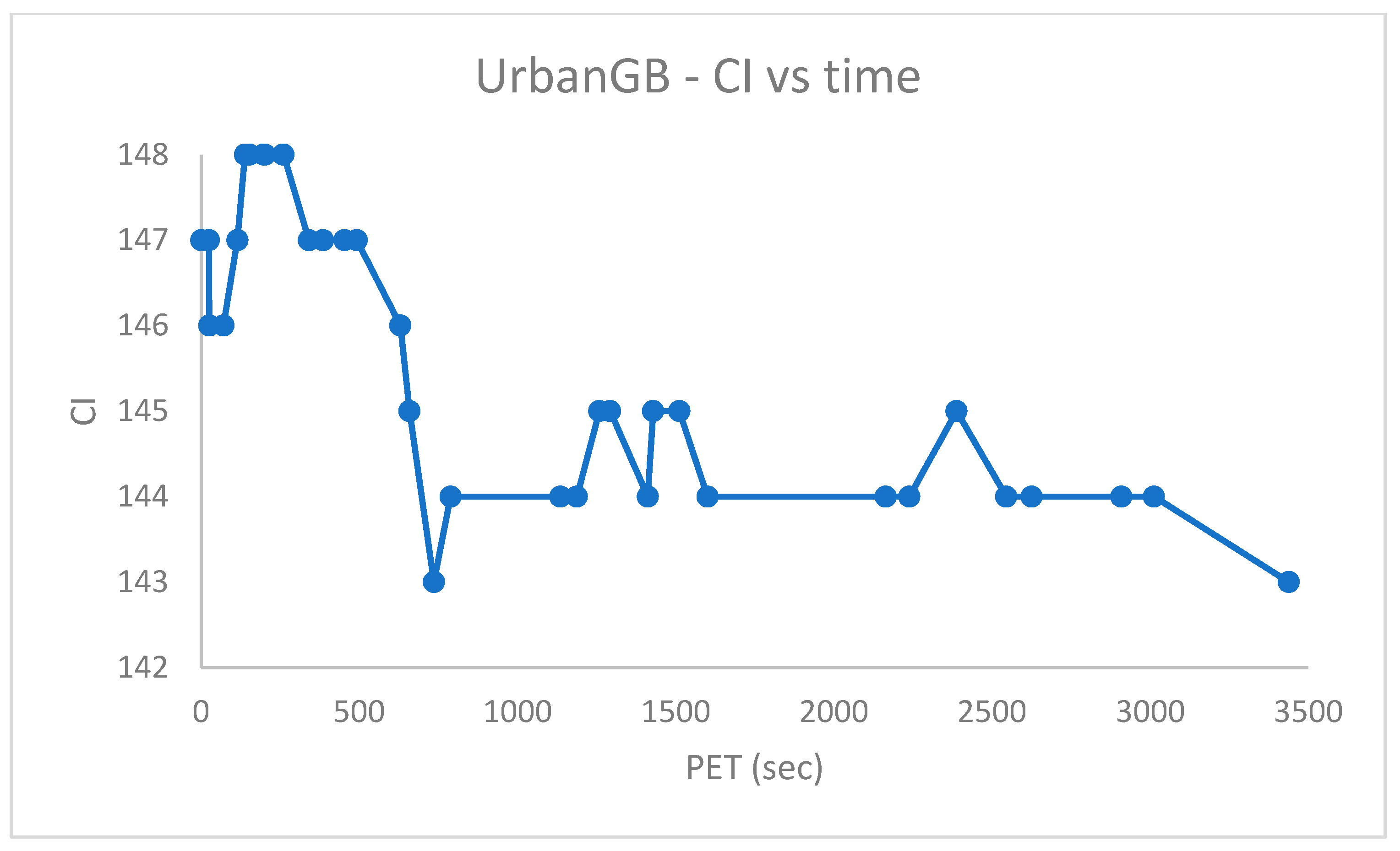28] datasets. Since $\mathrm{O}\mathrm{l}\mathrm{i}\mathrm{v}\mathrm{e}\mathrm{t}\mathrm{t}\mathrm{i}$ and $\mathrm{U}\mathrm{r}\mathrm{b}\mathrm{a}\mathrm{n}\mathrm{G}\mathrm{B}$are provided with ground truth information (both centroid and partition labels), Figure 14 and Figure 16 portray the observed centroid index $\mathrm{C}\mathrm{I}$ vs. time, respectively, for $\mathrm{O}\mathrm{l}\mathrm{i}\mathrm{v}\mathrm{e}\mathrm{t}\mathrm{t}\mathrm{i}$ and $\mathrm{U}\mathrm{r}\mathrm{b}\mathrm{a}\mathrm{n}\mathrm{G}\mathrm{B}$.

Figure 10. $\mathrm{S}\mathrm{S}\mathrm{E}$ vs. time for the $\mathrm{B}\mathrm{r}\mathrm{i}\mathrm{d}\mathrm{g}\mathrm{e}$ dataset.

Figure 11. $\mathrm{S}\mathrm{S}\mathrm{E}$ vs. time for the $\mathrm{M}\mathrm{i}\mathrm{s}\mathrm{s}\mathrm{A}\mathrm{m}\mathrm{e}\mathrm{r}\mathrm{i}\mathrm{c}\mathrm{a}$ dataset.

Figure 12. $\mathrm{S}\mathrm{S}\mathrm{E}$ vs. time for the $\mathrm{H}\mathrm{o}\mathrm{u}\mathrm{s}\mathrm{e}$ dataset.

Figure 13. $\mathrm{S}\mathrm{S}\mathrm{E}$ vs. time for the $\mathrm{O}\mathrm{l}\mathrm{i}\mathrm{v}\mathrm{e}\mathrm{t}\mathrm{t}\mathrm{i}$ dataset.

Figure 14. $\mathrm{C}\mathrm{I}$ vs. time for the $\mathrm{O}\mathrm{l}\mathrm{i}\mathrm{v}\mathrm{e}\mathrm{t}\mathrm{t}\mathrm{i}$ dataset.

Figure 15. $\mathrm{S}\mathrm{S}\mathrm{E}$ vs. time for the $\mathrm{U}\mathrm{r}\mathrm{b}\mathrm{a}\mathrm{n}\mathrm{G}\mathrm{B}$ dataset.

Figure 16. $\mathrm{C}\mathrm{I}$ vs. time for the $\mathrm{U}\mathrm{r}\mathrm{b}\mathrm{a}\mathrm{n}\mathrm{G}\mathrm{B}$ dataset.

From Figure 14, it emerges that the clustering algorithm could not recognize $7$ faces out of $40$. Similarly, the results in Figure 16 indicate that, in the best case, $143$ of $469$ cases were not correctly handled in the $\mathrm{U}\mathrm{r}\mathrm{b}\mathrm{a}\mathrm{n}\mathrm{G}\mathrm{B}$ dataset.

The shown experimental results agree with those reported in [11,12].

5.6. Time Efficiency of PB-KM

The computational efficiency of the developed tools was assessed, in a case, using the PB-KM recombination step on the $\mathrm{W}\mathrm{o}\mathrm{r}\mathrm{m}\mathrm{s}\_64\mathrm{d}$ dataset (see Table 4), via the GKM++ seeding method, with $\mathrm{J}=40$ and ${\mathrm{R}}_2=200$ repetitions, separately in parallel (the parameter $\mathrm{P}\mathrm{A}\mathrm{R}\mathrm{A}\mathrm{L}\mathrm{L}\mathrm{E}\mathrm{L} \mathrm{s}\mathrm{e}\mathrm{t} \mathrm{t}\mathrm{o} \mathrm{t}\mathrm{r}\mathrm{u}\mathrm{e})$ and sequential $\left(\mathrm{P}\mathrm{A}\mathrm{R}\mathrm{A}\mathrm{L}\mathrm{L}\mathrm{E}\mathrm{L}=\mathrm{f}\mathrm{a}\mathrm{l}\mathrm{s}\mathrm{e}\right)$ modes. The total elapsed time $\mathrm{t}\mathrm{E}\mathrm{T}$ (in msec) for the serial (${\mathrm{t}\mathrm{E}\mathrm{T}}^S$) and parallel (${\mathrm{t}\mathrm{E}\mathrm{T}}^P$) case needed by PB-KM recombination to complete were measured, together with the total number of executed K-Means iterations (respectively ${\mathrm{t}\mathrm{I}\mathrm{T}}^S, {\mathrm{t}\mathrm{I}\mathrm{T}}^P$), as reported in Table 10.

Table 10. The sequential and parallel execution of PB-KM recombination on ${\mathrm{W}\mathrm{o}\mathrm{r}\mathrm{m}\mathrm{s}}_{64\mathrm{d}}$. (8 physical cores).

$\mathbf{W}\mathbf{o}\mathbf{r}\mathbf{m}\mathbf{s}\_64\mathbf{d}$	$\mathbf{PB}-\mathbf{KM}, 2\mathbf{nd} \mathbf{Step}, \mathbf{J}=40$$, {\mathbf{R}}_2=100$
${\mathrm{t}\mathrm{E}\mathrm{T}}^S$ (ms)	4,405,325
${\mathrm{t}\mathrm{I}\mathrm{T}}^S$	15,049
${\mathrm{t}\mathrm{E}\mathrm{T}}^P$(ms)	650,622
${\mathrm{t}\mathrm{I}\mathrm{T}}^P$	14,887

From the data in Table 10, the average elapsed time per iteration was computed as ${av\mathrm{E}\mathrm{T}}_{it}^S=\frac{{t\mathrm{E}\mathrm{T}}^S}{{t\mathrm{I}\mathrm{T}}^S}=292.73$ and ${av\mathrm{E}\mathrm{T}}_{it}^P=\frac{{t\mathrm{E}\mathrm{T}}^P}{{t\mathrm{I}\mathrm{T}}^P}=43.70$, and the speedup was estimated as

$$\mathrm{s}\mathrm{p}\mathrm{e}\mathrm{e}\mathrm{d}\mathrm{u}\mathrm{p}={av\mathrm{E}\mathrm{T}}_{it}^S/{av\mathrm{E}\mathrm{T}}_{it}^P=\frac{292.73}{43.70}=6.7$$

6. Conclusions

This paper proposes two evolutionary-based clustering algorithms: Population-Based K-Means (PB-KM) and Population-Based Random Swap (PB-RS). The two algorithms were inspired by the Recombinator-K-Means [11,12] and the Genetic Algorithm of P. Franti [10], plus the use of the careful seeding ensured by the Greedy K-Means++ (GKM++) method [11,14].

However, PB-KM and PB-RS are based on a simpler, yet effective, approach which rests on two steps. In the first step, a population of $\mathrm{J}$ candidate “best” centroid solutions is created. The second step recombines the population’s centroids toward obtaining a careful solution. This is achieved in PB-KM through a number of independent repetitions of Lloyd’s K-Means [2,3,4], and in PB-RS by a certain number of iterations of Random Swap [8,9]. In both cases the starting point is a centroid configuration achieved by applying GKM++ to the population. Refinement of the initial solution is then controlled by partitioning the points of the dataset and moving toward minimizing the Sum of Squared Errors ($\mathrm{S}\mathrm{S}\mathrm{E}$) cost.

A key factor of PB-KM and PB-RS concerns their implementation in Java, which is based on parallel streams [9,15,16], which enables the exploitation of the parallel computing potential of modern multi/many-core machines.

The paper documents the reliable and efficient clustering capabilities of PB-KM and PB-RS by applying them to a collection of challenging benchmark and real-world datasets.

Ongoing and future work aims to address the following points.

First, it aims to experiment with the two developed algorithms for clustering sets [20,29] and more in general categorical and text-based datasets.

Second, it aims to port the implementations on top of the efficient Theatre actor system [30], which allows for better control and exploitation of the parallel resources of a multi/many-core machine.

Third, the aim is to adapt PB-KM by replacing Lloyd’s K-Means with the Hartigan and Wong variation of K-Means [31,32]. The idea is to experiment with an incremental technique which constrains the switching of a data point from its source cluster to a destination cluster also on the basis of its Silhouette coefficient [33]. The goal is to favor the definition of well-separated clusters.

The fourth aim is to compare the two developed algorithms to affinity propagation clustering [34] algorithms, e.g., for studying the seismic consequences caused by earthquakes [35]. In addition, the influence of the method about point distributions in the hypersphere [36] on our described clustering work deserves particular attention.