Article

On the Development of Descriptor-Based Machine Learning Models for Thermodynamic Properties: Part 2—Applicability Domain and Outliers

Université de Lorraine, CNRS, LRGP, F-54001 Nancy, France
*
Author to whom correspondence should be addressed.
Algorithms 2023, 16(12), 573; https://doi.org/10.3390/a16120573
Submission received: 20 October 2023 / Revised: 1 December 2023 / Accepted: 5 December 2023 / Published: 18 December 2023
(This article belongs to the Special Issue Nature-Inspired Algorithms in Machine Learning (2nd Edition))

Abstract

:
This article investigates the applicability domain (AD) of machine learning (ML) models trained on high-dimensional data, for the prediction of the ideal gas enthalpy of formation and entropy of molecules via descriptors. The AD is crucial as it describes the space of chemical characteristics in which the model can make predictions with a given reliability. This work studies the AD definition of a ML model throughout its development procedure: during data preprocessing, model construction and model deployment. Three AD definition methods, commonly used for outlier detection in high-dimensional problems, are compared: isolation forest (iForest), random forest prediction confidence (RF confidence) and k-nearest neighbors in the 2D projection of descriptor space obtained via t-distributed stochastic neighbor embedding (tSNE2D/kNN). These methods compute an anomaly score that can be used instead of the distance metrics of classical low-dimension AD definition methods, the latter being generally unsuitable for high-dimensional problems. Typically, in low- (high-) dimensional problems, a molecule is considered to lie within the AD if its distance from the training domain (anomaly score) is below a given threshold. During data preprocessing, the three AD definition methods are used to identify outlier molecules and the effect of their removal is investigated. A more significant improvement of model performance is observed when outliers identified with RF confidence are removed (e.g., for a removal of 30% of outliers, the M A E (Mean Absolute Error) of the test dataset is divided by 2.5, 1.6 and 1.1 for RF confidence, iForest and tSNE2D/kNN, respectively). While these three methods identify X-outliers, the effect of other types of outliers, namely Model-outliers and y-outliers, is also investigated. In particular, the elimination of X-outliers followed by that of Model-outliers enables us to divide M A E and R M S E (Root Mean Square Error) by 2 and 3, respectively, while reducing overfitting. The elimination of y-outliers does not display a significant effect on the model performance. During model construction and deployment, the AD serves to verify the position of the test data and of different categories of molecules with respect to the training data and associate this position with their prediction accuracy. For the data that are found to be close to the training data, according to RF confidence, and display high prediction errors, tSNE 2D representations are deployed to identify the possible sources of these errors (e.g., representation of the chemical information in the training data).

Graphical Abstract

1. Introduction

The adoption of QSPR/QSAR (Quantitative Structure Property/Activity Relationship) models has become very widespread for the prediction of various properties (e.g., physico-chemical, environmental, toxicological, safety-related) or activities (e.g., biological, pharmacological) on the basis of molecular structure. Being trained with a defined database of molecules, the applicability of these models to a new molecule is, however, limited to the so-called “applicability domain” (AD), i.e., the chemical structure and response space within which a model can make predictions with a given reliability [1]. The chemical structure refers to the structural and physico-chemical information that is provided by the descriptors, while the response corresponds to the predicted property or activity, namely the enthalpy of formation or the entropy, in the present study. This AD is crucial, as the final goal of QSPR/QSAR models is to be able to apply them for the prediction of the target endpoint of new molecules (i.e., not used during the model training and validation) and it is well known that the use of a ML model outside its training domain can be risky [2,3]. In other words, the more distant a point is from the training domain, the more unreliable the prediction. Driven by the motivation to generalize the usage of QSPR/QSAR models for regulatory purposes (e.g., REACH regulation for Registration, Evaluation, Authorization and Restriction of CHemicals), in 2004, the OECD (Organisation for Economic Co-operation and Development) defined a set of five principles for (Q)SAR validation, including the necessity to explicitly define the AD [4]. Nevertheless, this AD definition step is still being overlooked or poorly defined in many studies, as highlighted in [3,5]. However, knowing if a ML model is extrapolating or not will improve its acceptability and transparency, as is the case when investigating the explainability of a ML model. Indeed, some studies revealed a decrease in extrapolation performance with distance from the training domain, which can be more or less pronounced depending on the ML model [2,6,7]. Finally, there is also no clear overview about which method to employ to define the AD in a given problem, especially when dealing with high-dimensional data (e.g., descriptor-based QSPR/QSAR models can contain up to several tens, hundreds or thousands of descriptors). Most classical AD approaches are indeed dedicated to problems with few dimensions (i.e., less than ten), as will be discussed in Section 2.
The AD of a model is defined by the structural, physico-chemical and response information contained in the training data used to build the model [4]. Concretely, if a molecule lies outside the AD (i.e., extrapolation case, the molecule has low similarity with the molecules of training data), the prediction is more likely to be unreliable. However, even when properly defined, the AD should be considered cautiously since it does not constitute a strictly delimited space, meaning that the prediction for a molecule inside/outside the AD is not necessarily 100% reliable or false, respectively. Besides, it would be unrealistic to consider the existence of an explicitly defined frontier between reliable and unreliable predictions; one should rather approach this discussion from the viewpoint of a compromise between the size of the AD and the reliability of the predictions. For example, in the leverage method, which is a popular method for defining the AD, as will be described later, the frontier of the AD is generally fixed at a leverage value h * , as defined in Equation (1). However, the strict definition of this unique rule-of-thumb threshold value is not exempt from concerns [8] and, after all, expresses this compromise (i.e., increasing h * will reduce the reliability of the predictions and vice versa [4]).
A condition for a point to belong to AD in leverage method:
h h * = 3 ( p + 1 ) / n
where h is the leverage of a considered point, n is the number of molecules in the training set and p is the number of descriptors.
The notion of AD is closely related to the notion of an “outlier” or “anomaly”. Indeed, defining the AD frontier between “normal” and “abnormal” points is identical to detecting outliers. Many definitions of an outlier can be found in reported studies [9,10,11,12]; however, a common consensus is that the term "outlier" generally refers to a point of an ensemble that is “significantly different” from the remaining points of the same ensemble. Due to their equivalence, the terms “AD definition” and “outlier detection” are therefore used interchangeably in this study. Additionally, three types of outliers can be distinguished in QSPR/QSAR studies, namely X-outliers, y-outliers and outliers towards the model (Model-outliers) [13]. X-outliers and y-outliers are outliers in the descriptor space X and the response space y, respectively. As for Model-outliers, they correspond to the molecules for which the properties are poorly predicted by the QSPR/QSAR model and can therefore be detected only after model construction. Note that a point can belong to different categories of outliers simultaneously [14]. Note also that for a new query molecule (i.e., unknown response), only X-outlier detection methods are applicable.
More generally, even if the AD has an obvious role during the deployment of QSPR/QSAR models on new molecules, its definition remains essential at the different stages of the modeling procedure in which it fulfills different functions [1]. First, it is recommended to define the AD and eliminate the outliers as early as possible in a machine learning (ML) project, as some methods (e.g., dimensionality reduction, data scaling) are very sensitive to outliers. This initial AD definition step can be viewed as a data preprocessing step that removes outliers in order to improve the performance of the models. Then, during model construction, the AD definition can serve as a way to check whether the validation and test data are indeed within the AD defined by the training data, which is necessary as ML models are generally not reliable in case of extrapolation due to their data-driven nature. Finally, during model deployment, the AD can be used to judge the reliability of the prediction made by the model for a new query molecule. In this last case, as outliers are identified within new data, the outliers can also be referred to as novelties.
This article is the second of a series of articles aiming to construct QSPR models on the basis of ML techniques, ML-QSPR, while examining the different choices that are offered to the developer along the way and analysing the effects of each one. In the first article of the series, two ML-QSPR models were developed to predict two thermodynamic properties, namely the enthalpy of formation (H) and the absolute entropy (S) for the ideal gas state of molecules at 298.15 K and 1 bar [15]. The molecular descriptors were employed as features of the models to describe the structural and atomic characteristics of the considered molecules of the DIPPR (Design Institute for Physical Properties) database. Within an objective of discovering new chemicals for various applications, a wide range of chemical structures were considered in the training data as means to increase the AD of the developed models. The retained models were two Lasso (Least Absolute Shrinkage and Selection Operator) linear models with 100 descriptors, selected from an initial ensemble of approximately 2500 descriptors through a feature selection step based on a genetic algorithm (GA).
While the first article focused on the development of the QSPR approach from data collection to model construction, this second article aims at defining the AD of the developed models, characterized by their high dimensionality. In particular, three substudies are implemented, each corresponding to the AD definition at different stages of the QSPR procedure, as described previously; namely, the stages of data preprocessing, model construction and model deployment. Therefore, in the first part of this study (referred to here as “substudy”), the AD definition is used as a data preprocessing method, in addition to the methods implemented in the first article, to remove outliers. At this stage, the number of descriptors is particularly high, with about 2500 descriptors. Several outlier detection methods are compared and the influence of the elimination of the identified outliers on the performance of the ML models is evaluated. All the types of outliers (i.e., X-outliers, y-outliers and Model-outliers) are considered. While y-outliers and Model-outliers are detected via boxplots (interquartile range method or IQR) and standardized residuals, respectively, X-outliers are identified on the basis of three simple methods having promising compatibility with high-dimensional problems. These methods are isolation forest (iForest), random forest-based confidence estimation (RF confidence) and k-nearest neighbors in a 2D projection of the descriptor space obtained via t-Distributed Stochastic Neighbor Embedding (tSNE2D/kNN).
In the second substudy, the most appropriate AD definition method, as identified within the first substudy, is employed to visualize the location of the test data with respect to the AD defined by the training data. Finally, in the last substudy, the goal is to attempt a concrete deployment of the developed ML-QSPR model to new species, including the prediction and the analysis of the reliability of the predictions in terms of the AD, still based on the AD definition method identified in the first substudy. In the last two substudies, as they occur after dimensionality reduction, they rely on fewer descriptors, namely the 100 descriptors selected by means of a GA applied on the preprocessed data without outliers. Additionally, for these same substudies, further analyses are also provided regarding the potential sources of high prediction errors.

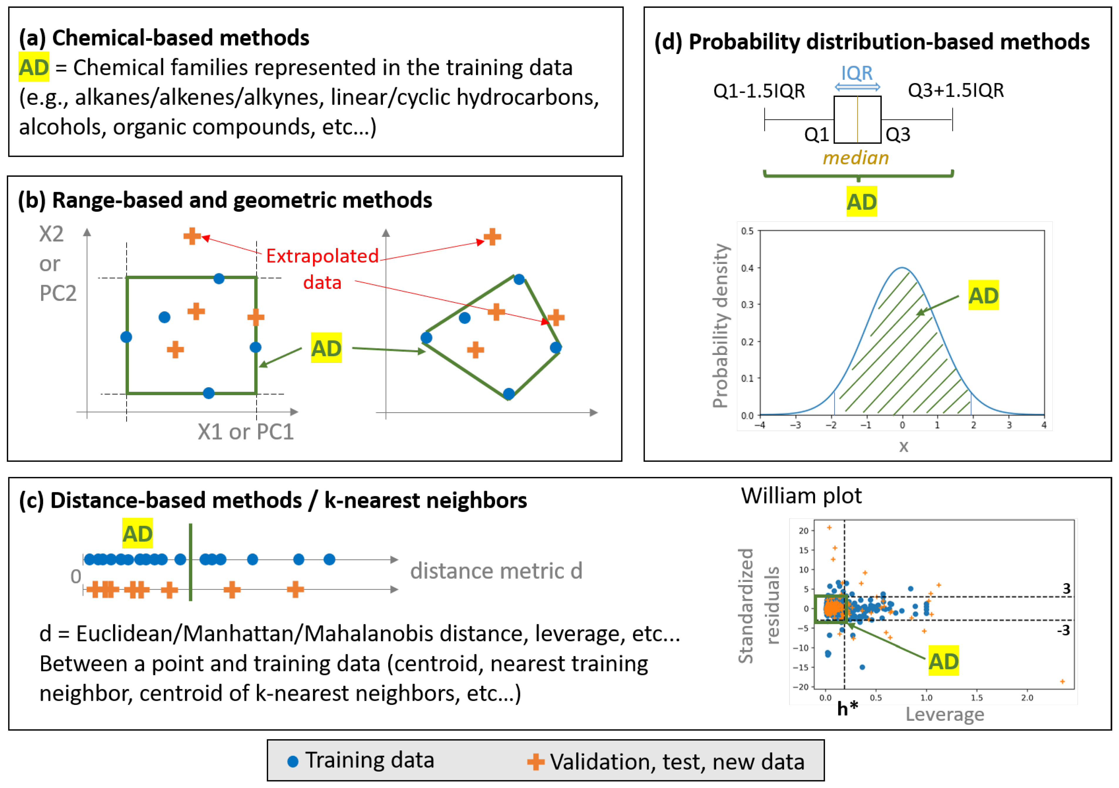
2. Overview of the Methods for AD Definition/Outlier Detection in Descriptor-Space and Their Compatibility with High-Dimensional Data

In this section, an overview of the methods for AD definition (or outlier detection) is provided, with a focus on X-outliers. The latter are effectively the most challenging to identify in view of their high dimensionality. First, the methods that are commonly employed to define the AD of QSPR/QSAR models are presented. These methods can be classified in different categories, including chemical-based methods, range-based methods, geometrical methods, distance-based methods and probability distribution-based methods, as illustrated in Figure 1. As these have already been exhaustively reported and described in several works [1,16,17,18,19], only a quick overview is provided here, for reasons of completeness, placing special emphasis on the low compatibility of these methods with high-dimensional data. Besides, they are generally applied during model construction or deployment. Inversely, other methods for outlier detection in high dimension, presented secondly here, including confidence estimation-based methods, subspace-based methods and other specific methods (e.g., iForest), are more suitable to the characteristics of the three substudies investigated in this work.

2.1. Classical Approaches

A typical approach that is commonly employed in QSPR/QSAR studies involving different molecules is to consider that the AD corresponds to the chemical families on which the model was trained [20,21,22,23]. This approach, otherwise known as “chemical-based”, relies on the premise that the predicted property will explicitly depend on the molecular characteristics that are used to define the chemical families (e.g., type of bonds, presence of rings or functional groups, etc.), a dependence that is not always guaranteed a priori.
“Range-based” methods use the range of each descriptor within the training data to define the AD as a hyper-rectangle of dimension equal to the number of descriptors [1]. Despite their simplicity, the major problem of range-based methods lies in the presence of empty spaces inside the hyper-rectangle making the AD description quite rough. This is even more pronounced for high-dimensional data, where points tend to become equidistant as the number of dimensions increases [9]. Empty spaces do not contain any training data and can be particularly wide in the presence of outliers. This could therefore call into question the reliability of future predictions in these regions, even though they are part of the AD. To limit the extent of the empty spaces caused by the high dimensionality, range-based methods can also be applied to descriptor-derived representations of lower dimension, such as the principal components (PC), issued by the prior implementation of a Principal Component Analysis (PCA). This combination also addresses eventual collinearities within the descriptor space.
In “geometric methods”, the AD corresponds to a convex hull, as this is the smallest convex area that contains the entire training set. In a 2D space, the convex hull can be easily understood via the rubber band analogy: the rubber band tautly surrounding the training set descriptors is the convex hull. Similarly as for range-based methods, empty spaces are not detected. What is more, the calculation of the convex hull becomes computationally complex in high dimensions. In fact, as higher dimensions lead to a higher extrapolation probability [24], both geometric and range-based methods will very likely consider any new point as being outside the AD (i.e., the new point will most probably be extrapolating in at least one dimension).
“Distance-based methods” are among the most commonly used. They rely on the calculation of a distance-based metric between a given point and the training set. If the distance is below a defined threshold, the point is considered to be part of the AD and vice versa. Among popular distance metrics, one finds the Euclidean and Mahalanobis distances. The latter is popular for the detection of outliers in multivariate data, as is the case with the descriptor space [25]. Contrary to the Euclidean distance, it can identify correlations between features by means of the covariance matrix, similarly as in PCA. Graphically, the AD shape in the case of Mahalanobis distance will be more extended in the directions containing the highest variance (ellipse in 2D), and this will avoid the deletion of points that are not real outliers, as in the case of Euclidean distance (circle in 2D) [26].
Another approach that is popular in recent works is the so-called “leverage method” [1,16,27,28,29,30,31,32]. In these works, the number of features is variable, ranging from less than 10 (principally) to several hundreds or thousands (less frequently). In analogy to the Mahalanobis distance [33], the leverage quantifies the distance between a given point and the centroid of the training data X, in terms of its feature values, and provides an estimation of the potential influence that the observed response will have on its predicted value. Mathematically, the leverage values of the training samples X can be obtained via the diagonal elements h i i of the hat matrix H, as defined by Equations (2) and (3). For a new query sample x n e w , the leverage values are calculated via a similar formula, defined by Equation (4). From these equations, it is possible to identify that the major problem in the leverage method will be related to the inversion of the matrix X T X . This inversion becomes problematic when the descriptor matrix X contains redundant or correlated information, or when the number of descriptors exceeds the number of samples [26]. Besides, the calculation of the matrix X T X is sensitive to outliers, as highlighted in [25,34].
Hat matrix H and leverage values h i i , h n e w :
H = X ( X T X ) 1 X T
h i i = x i T ( X T X ) 1 x i
h n e w = x n e w T ( X T X ) 1 x n e w
where X is the descriptor matrix based on training data (with n rows/observations and p columns/descriptors), x i is the column vector of a molecule in the training data and x n e w is the column vector of any new molecule.
In practice, leverage values (X-outliers) are plotted against standardized residuals (Model-outliers) on a Williams plot, with their corresponding thresholds. Standardized residuals are defined by Equation (5). Generally, a point belongs to the AD if its leverage value is below h * = 3 ( p + 1 ) / n and if its standardized residual is between −3 and 3 [35,36]. These user-defined rule-of-thumb thresholds can be understood as follows. For the leverage threshold, the idea is that one compares the value of the leverage of a single point with the mean leverage value of all points, ( p + 1 ) / n . As for standardized residuals, the cutoff value of ± 3 covers 99% of the assumed normally distributed standardized residuals. Williams plots are more a graphical way to verify whether a developed model is statistically acceptable during model construction [29,36]. However, it is only possible to check if a new query molecule is an X-outlier, and not if it is a Model-outlier, as the calculation of the standardized residual is impossible (i.e., the observed property value is unknown).
Standardized residuals:
r k = y k o b s e r v e d y k m o d e l V a r ( r t r a i n )
where y k o b s e r v e d and y k m o d e l are, respectively, the observed and the predicted responses for a molecule k and V a r ( r t r a i n ) is the variance of residuals of the training data.
Other distance-based methods also include techniques that utilize the k-Nearest Neighbors (kNN) algorithm. In this case, it is the distance to the nearest training point or the average distance to the k-nearest training neighbors that can be used as a means to decide whether a point lies inside or outside the AD [16]. Similar to range-based and geometric methods, empty spaces remain undetected with distance-based methods. Most importantly, all these methods suffer from the consequences of the curse of dimensionality. As the number of descriptors increases, points become equidistant whatever the chosen distance metrics. Despite several attempts to develop distance metrics that are more compatible with high-dimensional data [11], it is far more common to use dimensionality reduction methods instead. Finally, another way to improve the AD definition when using distance-based methods is to calculate the distance metrics by considering different weights for the descriptors according to their influence (e.g., coefficients in linear regression) [1].
A different class of AD definition methods is based on the use of probability density distributions. Contrary to all previous methods, this is the only class of methods that can identify empty zones inside a convex hull. Indeed, the probability density function of the training data is first estimated via a parametric or a non-parametric method. Whenever possible, the latter is generally preferred, as it does not make any assumption about the shape of the function and learns it from the data. Then, the smallest region containing a given amount of the total probability is identified as the AD. Probability density distribution-based methods can be applied to multivariate data, but their application is often limited to three dimensions. For higher-dimensional problems, these methods become computationally expensive and some assumptions are generally required. To consider both feature and response spaces, it is also possible to use joint probability distributions to define the AD. In lower dimensions, if all features are normally distributed, a popular method consists of using boxplots (IQR method), in which the points outside the AD are those located below/above the lower/upper thresholds. These thresholds are, respectively, Q 1 1.5 × I Q R and Q 3 + 1.5 × I Q R , where Q 1 and Q 3 are the first and third quartiles, respectively, and I Q R = Q 3 Q 1 is the interquartile range. Once again, in higher-dimensional problems, it becomes more probable that any new molecule extrapolates for at least one descriptor, similar to the range-based and geometric methods. In [19], an approach based on the Z-score of the descriptors was proposed with an additional criterion to deal with this problem in high dimension. Despite its simplicity, this approach is also applicable strictly in cases where the descriptors are normally distributed.

2.2. Approaches for High-Dimensional Data

To overcome the limitations of the previously described approaches, when it comes to high-dimensionality problems, ML methods including an estimation of the confidence of the predictions in their output (e.g., Gaussian Processes, ensemble models like Random Forest) can be employed to detect outliers. For example, [37] used an embedded AD approach, based on the probabilities assigned to the output classes of a neural network classifier, as an effective approach to analyze the likelihood of correct predictions. In other words, if the likelihood of correct prediction is low for a molecule, then the latter is likely to be an outlier. Technically, a softmax layer was applied to the network outputs to obtain the probability of each class for each molecule, where the feature space was composed of 1500 to 3700 descriptors approximately. Similarly, in [38], the predictions made by an ensemble of classification decision trees were used to evaluate the confidence of the final prediction for a molecule, and therefore the outlier character of that molecule. More concretely, the fraction of trees that voted for the majority vote was used as the confidence (or probability) of the prediction. The method was applied to problems dealing with a feature space of approximately 100 to 1000 dimensions and showed significant robustness towards the high dimensionality, in comparison to the classical Euclidean distance-based approach. The same methodology can also be implemented via an ensemble of regression trees (or of other regression models), by using the variance of the predictions as a measure of the reliability of the final prediction (i.e., the average of the predictions of the ensemble of trees) [39,40].
Gaussian Processes (GP) can also be exploited for confidence estimation. In fact, GP defines a class of ML models that are based on the prediction of a posterior distribution of functions, characterized by their mean and variance [41]. This variance can therefore be used as a measure of the reliability of a prediction. In [39], an ensemble of regression trees (RF) and GP models outperformed classical approaches in the definition of the AD. Similarly, in [42], the AD definition via confidence estimation showed better results than the other investigated methods. All these techniques are based on the confidence estimation of ML predictions and on a less binary (i.e., inside/outside AD) approach to dealing with the definition of an AD, in comparison to classical AD methods, by providing a more shaded evaluation of the prediction reliability according to different levels of confidence. This characteristic renders them more compatible with high-dimensional problems.
Among the different outlier detection techniques that can be employed in high-dimensional problems, the methods based on projections in lower-dimensional subspaces are also very popular. In [9], a point was considered an outlier if there was a lower-dimensional subspace where this point would be located in a region of abnormally low density. To avoid an exponential search of relevant subspaces, evolutionary algorithms were implemented. Additionally, the density was obtained by dividing the space into grids and then calculating a density coefficient (the sparsity coefficient) for each cell of the grids. Other works used different projection techniques, such as PCA, axis parallel subspace spanned by a point’s neighbors or Hilbert space-filling curve, generally followed by a classical distance- or density-based technique, such as kernel density estimation or distance to the k t h nearest neighbor(s), to identify outliers [43,44,45,46,47].
More specific methods, without projection to a subspace of lower dimension, can also be found in the literature. For example, [48] exploited angles as a measure for detecting outliers, instead of distances, as the latter are very sensitive to high-dimensional data. Concretely, at a first step of this approach, the variance in the angles between the difference vectors of one point to the rest is calculated. If the variance is small, the analyzed point is considered an outlier, as most of the other points are located on one side (or in the same direction) of the analyzed point. In [49], an isolation-based anomaly detection method, called “isolation forest” (iForest), was developed to detect anomalies without using any distance or density measure, hence its compatibility with high-dimensional problems. The principle is simple, as it is based on random forest (RF). In RF, each tree splits the whole data (root node) into smaller and smaller groups until reaching leaf nodes, on the basis of decision rules at internal nodes. In iForest, the number of random splits to isolate a point is used to determine whether this point is an outlier or not. If the number of splits is low, the point is considered an outlier and vice versa. Indeed, it is easier to isolate a point that is located in a sparse region than another one that is part of a dense cloud of points. Similar to RF, an ensemble of trees is built to obtain an average number of splits to isolate each point. Another advantage of this method is that it can be readily implemented via the Scikit-Learn library in Python. Additional examples on both subspace-based and full-space-based methods for outlier detection in high dimensions can be found in [11,50,51], while further discussion on the effects of high dimensionality is available in [50,52,53].

3. Dataset and Methods

3.1. Dataset and ML/QSPR Models

In the previous article, two ML-QSPR models were built for the ideal gas phase standard enthalpy of formation and entropy, based on data from the DIPPR database [15]. These properties will be denoted as enthalpy (H) and entropy (S) in the rest of this article, for simplicity. Each molecule was represented by a vector of 5666 descriptors calculated using the software AlvaDesc from Alvascience [54,55]. After a series of preprocessing steps, the dataset was finally composed of 1785 molecules × 2506 descriptors for the enthalpy and of 1747 molecules × 2479 descriptors for the entropy. This dataset will be referred to as the “preprocessed data” in the rest of this article. More precisely, data preprocessing was composed of the following steps: elimination of the missing values, elimination of quasi-constant descriptors and elimination of correlations among descriptors. Finally, in this previous article, the number of descriptors was further reduced to 100 via a GA-based dimensionality reduction step to improve the interpretability of the models, in comparison to the initial 2506 or 2479 descriptors (for enthalpy and entropy, respectively). Further reduction of the number of descriptors is possible, but at the cost of prediction accuracy. A large diversity of molecules was also considered to broaden the AD. The best performing models turned out to be Lasso (Least Absolute Shrinkage and Selection Operator) models, based on the results averaged over five different train/test splits and in comparison with the different screened ML models. At last, a hyperparameter optimization step was also performed; however, this will not be considered in this article, as the main focus here is understanding the AD definition (or outlier detection) in a high-dimensional problem.

3.2. AD Visualization

The AD corresponds to the chemical structure and response space within which a model can make predictions with a given reliability. In this work, the AD will be graphically represented according to the template shown in Figure 2, and referred to as “AD plot”. The representation is highly inspired by William plots, but by replacing the leverage on the x-axis with another distance (or X-outlier) metric, it becomes more compatible with high-dimensional data, as will be presented in the next section. This x-axis refers to the “chemical structure space” of the AD definition given previously.
On the y-axis, the same standardized residuals as those described in William plots are considered. The combination of x- and y- axis permits us to visualize the chemical structure space within which a model can make predictions with a given reliability. In other words, it shows the success of prediction of the molecule structures considered as being part of the AD. In case of poor prediction, the concerned molecules can be considered as Model-outliers.
Additionally, a color bar can be used to visualize the property values of DIPPR data, referring to the “response space” in the AD definition and highlighting eventual y-outliers (the points with dark circles in Figure 2 are y-outliers according to the IQR method). The response space is not represented/investigated in the leverage method. Indeed, it is not possible to know if the property value of a new molecule is included in the range of property values of the training data. Besides, the extrapolation capacity of a ML model normally concerns the X-space and not the y-space. In the case of QSPR/QSAR studies, which are based on the similarity principle (i.e., similar structures lead to similar response values), X- and y- spaces are, however, somehow related. As part of this study, y-outliers will be briefly investigated.
While in the leverage method, the AD borders are defined according to widely employed rules-of-thumb, as described earlier, the borders in the case of the investigated AD methods for high-dimensional problems will be further evaluated in this work. Nevertheless, in the following section, all AD plots display the lines y = 3 and y = 3 , similarly as in William plots for reasons of legibility.

3.3. AD Definition as a Data Preprocessing Method (Substudy 1)

The first part of this work lies in the identification of the outliers in the preprocessed data through different AD definition methods and the evaluation of how the elimination of these outliers may impact the performance of the models. Depending on the type of outliers, different methods are employed.
For X-outliers, three methods are compared: isolation forest (iForest), random forest-based confidence estimation (RF confidence) and k-nearest neighbors in a 2D projection of the descriptor space obtained via t-Distributed Stochastic Neighbor Embedding (tSNE2D/kNN). Each of these methods can effectively be exploited to calculate anomaly scores for all the molecules, and were identified as common methods for outlier detection in the presence of high-dimensional data in Section 2.2. Then, the molecules with an anomaly score above a given threshold are eliminated. For iForest, it is represented by an anomaly score [49], which is negatively correlated to the average number of splits necessary to isolate a given point: the higher the anomaly score, the lower the number of splits, and the more isolated and the more abnormal the point of interest. As for RF confidence, the standard deviation of the individual trees’ predictions serves as a judgement basis of the reliability of a prediction provided by the ensemble of trees: the higher the standard deviation, the less reliable and the more abnormal the point. Indeed, a high standard deviation means that the individual trees are associated with very different predictions for the same sample, i.e., they are not able to “agree” on a reliable final prediction because the sample is too complex (e.g., specific/outlier behavior of the sample). For tSNE2D/kNN, the anomaly metric used is the average Euclidean distance of a point to its three nearest neighbors. The higher the distance, the more abnormal the point considered. In particular, this Euclidean distance is computed in the tSNE 2D space, tSNE being a nonlinear dimensionality reduction method principally used for data visualization in a 2D or 3D space [56]. Finally, note that all three X-outlier detection methods were applied with Scikit-Learn default parameters.
Concerning y-outliers and Model-outliers, they were identified via the IQR method and standardized residuals, respectively (see Equation (5)). In the case of the IQR method, y-outliers are the points located outside the thresholds of Q 1 1.5 × I Q R and Q 3 + 1.5 × I Q R , as explained previously. For Model-outliers, the molecules with absolute standardized residuals above a given threshold were considered as outliers. The residuals were obtained via a Lasso model trained on the whole preprocessed data. Note that the molecules identified as Model-outliers here are not strictly Model-outliers as defined in the introduction. Indeed, the latter are identifiable only after model construction (i.e., after eventual dimensionality reduction followed by model training and validation), while here we are still at the preprocessing stage. This can be viewed as a preventive treatment, since a late detection of Model-outliers would lead to a necessity to repeat dimensionality reduction and model construction steps after removal of the “real” Model-outliers.
To evaluate the impact of the outliers on the performance of the models, different thresholds were implemented to eliminate the outliers according to the aforementioned detection methods. Then, the resulting preprocessed data without outliers were split into training and test sets, the ratio between them being fixed at 80:20, and scaled via a standard scaling method. This ratio for data splitting and this scaling method were indeed identified as well performing in the first article of the series [15]. To better integrate the effect of data splitting on the performance of the models, five different training/test splits were considered. These five splits were defined so that each molecule belongs to the test set exactly once among the different splits. Note that outlier elimination was performed on preprocessed data and before data training/test splitting in order to keep the training/test ratio intact. Finally, the Lasso models were trained and validated for each of these splits, without performing dimensionality reduction. In the results section, the presented model performances are averaged over these splits, and the error bars displayed on the figures are the corresponding standard deviations. The considered performance metric is the mean absolute error ( M A E ).
In particular, four configurations are implemented and compared, as summarized in Table 1. In the first configuration, the effect of X-outliers is investigated. For each X-outlier detection method, different amounts of X-outliers are eliminated from the preprocessed data, namely 0%, 10%, 30% and 50% (based on anomaly score). The subsequent preprocessed data without X-outliers, for the different elimination thresholds and X-outliers detection methods, are then submitted to data splitting, scaling and model training/test, as described in the previous paragraph.
Concerning the second configuration, the effect of Model-outliers is studied via a procedure similar to that adopted for the X-outliers. The only difference lies within the tested standardized residual thresholds, namely 1, 2, 3, 5 and 10, in absolute values. This means that molecules with absolute standardized residual value above 1, 2, 3, 5 and 10 are removed from the preprocessed data.
In the third configuration, the combined effect of X-outliers and Model-outliers is analyzed. In particular, the three following layouts are compared, for a given X-outlier detection method (RF confidence) and for given thresholds in the detection of X-outliers and Model-outliers:
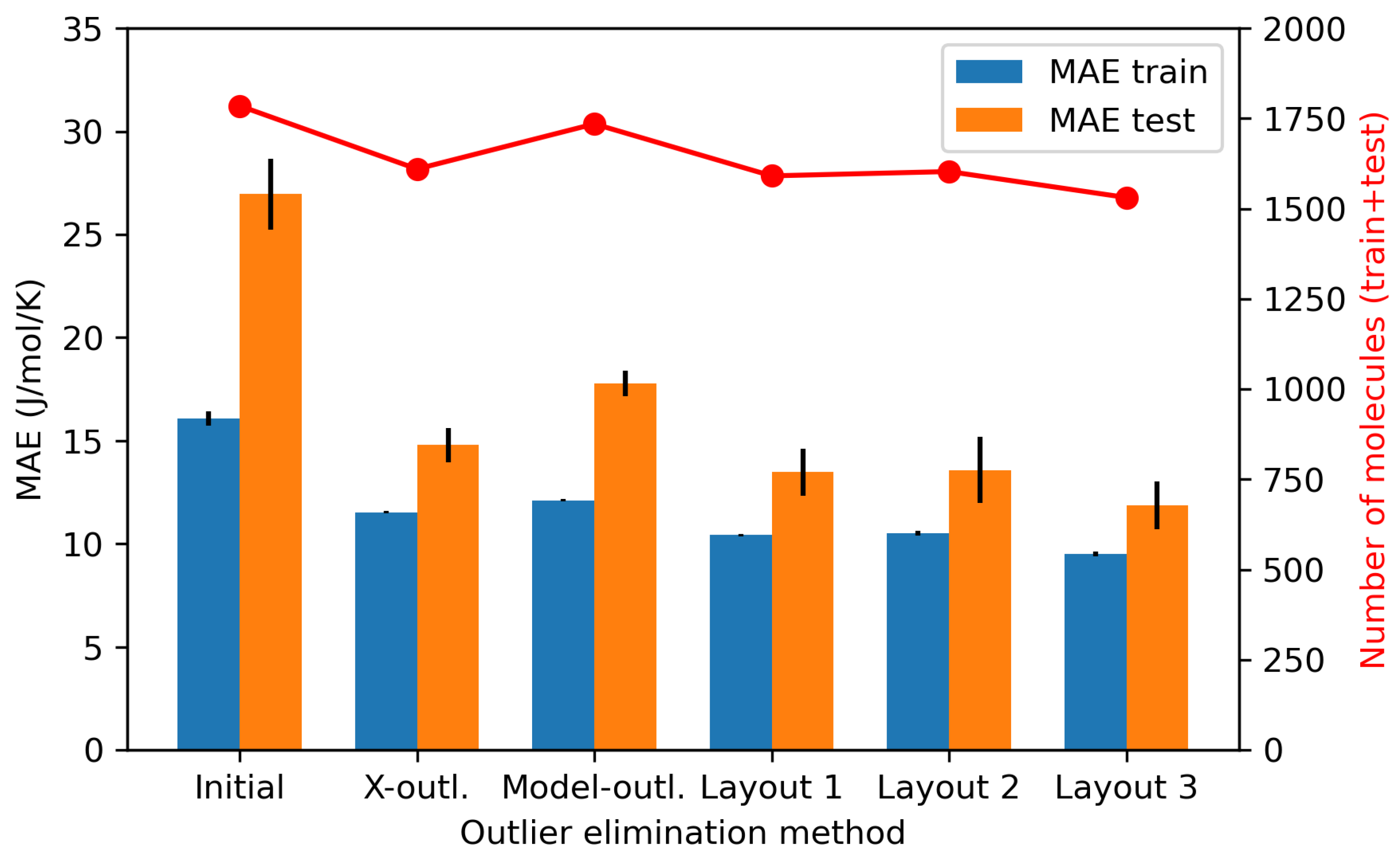
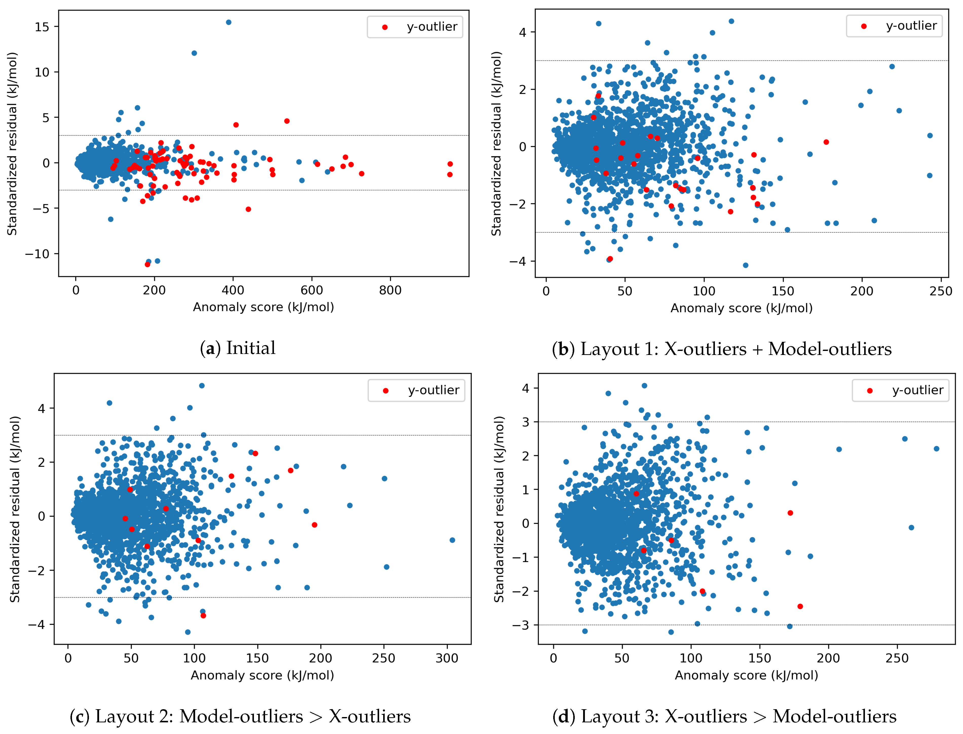
  • Layout 1: simultaneous elimination of X-outliers and Model-outliers.
  • Layout 2: elimination of Model-outliers followed by elimination of X-outliers.
  • Layout 3: elimination of X-outliers followed by elimination of Model-outliers.
Finally, for y-outliers, the thresholds are those as defined earlier using the IQR method, and the effect of their elimination on the model performance is analyzed.

3.4. AD Definition during ML Model Construction (Substudy 2)

Once the best-performing outlier detection method has been identified and the outliers eliminated (substudy 1), the obtained dataset, preprocessed and without outliers, is subjected to the previously presented data splitting and data scaling steps. Furthermore, a dimensionality reduction step is implemented to improve interpretability of the developed ML models. To achieve this, the same GA procedure as the one used in the first article is used to reduce the numbers of descriptors to a fixed number of 100 [15]. Finally, the Lasso models are trained and validated on the new dataset of reduced dimension. Note that the criterion of selection of the best-performing outlier detection method is based on compromise between high training/test performances and the lowest possible number of eliminated molecules.
The main goal of this second substudy is to visualize where the test data are located with respect to the AD defined by the training data. Therefore, the AD of each model is visualized on AD plots showing the standardized residuals (Model-outliers) of the different molecules versus their anomaly scores (X-outliers). The test data should be within or close to the AD to have a reliable model.
In addition to the above, tSNE 2D representations are provided in an attempt to identify the potential sources of high prediction errors (e.g., lack of training molecules in certain regions, presence of molecules with different structures but similar property values...). Note that the procedure of this substudy also applies to a potential hyperparameter optimization phase in order to check whether the validation data are indeed close to the training data. However, this study has not been pursued in the framework of the present article.

3.5. AD Definition during ML Model Deployment (Substudy 3)

The goal of this final substudy is to show a concrete deployment of the developed ML-QSPR models to new species (i.e., those not used for model training and validation), including the prediction and the analysis of the reliability of the predictions with respect to the defined AD. In this sense, the models resulting from substudy 2, based on the preprocessed data without outliers and with dimensionality reduction, are deployed to predict the properties of new species. These are classified into four different categories, namely Cat. A (13 species), Cat. B (5 species), Cat. C (45 species for enthalpy, 44 species for entropy) and Cat. D (12 species). Due to confidentiality issues, no further information about the chemistry of these species can be provided. The descriptor values for these new species were calculated by AlvaDesc (v2.0.8) on the basis of the optimized geometry, in MDL MOL format (containing information on atom coordinates/types and on bond types), calculated by the software Gaussian 09 (revision B.01) [57]. Calculations were performed at the CBS-QB3 level of theory [58] and conformational analysis was conducted in a systematic way to be sure to identify the structure with the lowest energy (this was performed at the B3LYP/6-31G(d) level [59]). Raw data provided by the software Gaussian were then post-processed using the GPOP software suite from Miyoshi [60] to derive the thermodynamic properties (enthalpy and entropy). The contribution of internal rotations of moieties around simple bonds was corrected by considering the hindered rotor model rather than the harmonic oscillator one when the potential energy was less than 10 kcal/mol. Note that the calculations could not be performed for all species contained in Cat. C, resulting in 21 and 39 species with available Gaussian-calculated properties in Cat. C, for H and S, respectively.
The reliability of the predictions is subsequently analyzed in relation to the distance of the new species to the AD. Again, the AD is visualized on AD plots, showing the species’ standardized residuals (Model-outliers) and RF confidence-based anomaly scores (X-outliers). Note that, in practice, the properties of new species are unknown; hence, their standardized residuals are also unknown. In this work, the enthalpy and/or entropy of the new species were calculated by DFT on Gaussian to serve as reference values for comparison with the predictions. The availability of the standardized residuals for the new species is utilized to improve the understanding and analysis of the AD. Besides, similarly as in substudy 2, tSNE 2D representations are also provided to try to identify the potential sources of high prediction errors.
All the ML models of this work were implemented using the Scikit-learn library v1.0.2 of Python v3.9.12.

4. Results

4.1. AD Definition as a Data Preprocessing Method (Substudy 1)

The analysis of AD definition methods during data preprocessing was investigated for the enthalpy QSPR model and is presented below. As for entropy, the best-performing AD definition method, identified for the enthalpy, is applied to eliminate the outliers. All the results are provided below.

4.1.1. Outlier Detection

X-outliers, y-outliers and Model-outliers are detected on the preprocessed data via the different methods presented in Section 3.3. Figure 3a–c show a visual representation of the preprocessed data for the enthalpy only, according to the different categories of outliers, as well as according to the three studied methods for X-outlier detection. In particular, the x-axis corresponds to an anomaly score specific to each X-outlier detection method, while the y-axis corresponds to the standardized residual between the reference response value (DIPPR) and the predicted one by the Lasso model trained on the whole preprocessed data. Points identified as y-outliers are colored in red. Note that the implementation of the leverage method for X-outlier detection is not presented here due to the occurrence of numerical issues in the calculation of the hat values, probably due to existing multicollinearities between the descriptors (more than 2000 descriptors) that resulted in negative eigenvalues of the matrix X T X [26,61]. This is evidence of the limitations of the leverage method when applied to high-dimensional data. In addition, tSNE was preferred over PCA for projecting the descriptor space into a lower-dimensional space, since the number of PCs necessary to describe 95% of the data variance exceeds 200, with the first component containing only 20% of the variance (the numbers given are for the enthalpy, but the situation is similar for the entropy).
For all three X-outlier detection methods, similar behavior can be observed in Figure 3a–c. Points showing a high score in the abscissa metric (i.e., considered as the “most abnormal” in descriptor space) tend to be better predicted (i.e., with lower absolute standardized residual values) than some points with lower abscissa values. It seems as if, even though these points are located “further away” in the descriptor space (i.e., in terms of the employed metric) than the majority of data, the model succeeds in “extending” the response hypersurface to include them [33].
The molecules displaying the highest absolute standardized residuals (Model-outliers) and the highest anomaly scores (X-outliers), according to the three investigated detection methods, are shown in Table A1 and Table A2, respectively. The first category (i.e., Model-outliers) mainly includes molecules containing halogen, polyfunctional and silicon compounds, while in the second category (i.e., X-outliers) it is seen that iForest and RF confidence identify some common molecules, such as large silicon or halogen compounds. All these identified families share a common element of being poorly represented, as there is a lack of molecules containing the characteristic heteroatoms of these families in the database. This could be one of the reasons for their identification as outliers; for example, they can be easily isolated (iForest) or display high standard deviations in the individual trees’ predictions (RF confidence). Note also that polyfunctional compounds combine several functional groups, thus conferring to these molecules a partial similarity, in terms of some descriptor values, to other species that also contain these groups, despite their overall different structures and enthalpy and/or entropy values. Additionally, for the two first molecules of Table A1, with chemid n°3608 and 2628, another explanation for their outlier behavior could be related to the significant difference (i.e., of 700 and 600 kJ/mol, respectively) that is observed in their enthalpy values with their counterparts with the same formula. Finally, concerning X-outlier detection, tSNE2D/kNN does not seem to share any molecule in common with the two other methods. This is mainly due to the completely different mechanism that is employed by this method, where the molecules identified as X-outliers are the most isolated ones from the clusters that are formed in the tSNE 2D space, in contrast to tree-ensembles that are employed by iForest and RF confidence. The effects of both X-outliers and Model-outliers on the model performance are further investigated in the following parts.
Concerning y-outliers, it is seen in Figure 3a–c that, when RF confidence is employed, these are mostly located in the areas with high anomaly scores, outside the cluster with a high density of points. Accordingly, their elimination can be carried out via the elimination of X-outliers in this case. Figure 3d, where the RF confidence plot is reproduced, coupled with a color scale indicating the enthalpy values of the molecules, seems to confirm that a high percentage of both X- and y-outliers is displayed by molecules of lower enthalpy values. This observation, in conjunction with the distribution of enthalpy values in the dataset (cf. the first article of the series [15]), corroborates the hypothesis of poor representation of these molecules in the dataset (e.g., very large molecules). In this case, the elimination of these points is questionable. In fact, points from poorly represented domains may be useful to a model whose applicability will need to include such molecules. In the case of entropy, the elimination of y-outliers via the one of X-outliers does not seem feasible, as shown in Figure 4, where a non negligible amount of y-outliers is contained in the area with low RF confidence anomaly scores, within the cluster with a high density of points. This could be related to the eventual existence of property cliffs, namely molecules that have similar descriptor values but very different property values, thus posing significant problems for QSPR/QSAR modeling studies, as these rely on the similarity principle [62]. The existence of such issues in the dataset is also evidence of the limitation of the descriptor-based molecular representation approach in these studies.
Finally, looking at Figure 3 and Figure 4, it seems that, for RF confidence, the regions with the lowest anomaly scores seem to contain less molecules with high absolute standardized residuals, which are located in a less dense region with higher anomaly scores. This effect is particularly visible for entropy. All these elements highlight a possible relation between RF confidence anomaly score and high prediction errors, which could be exploited during ML model deployment to new species to assess the reliability of the predictions. In other words, the aim is to investigate whether a new species with a low RF confidence anomaly score is more likely to provide more reliable model predictions and the opposite.

4.1.2. Effects of X-outliers on the Model Performance

To better understand the effects of X-outliers on the performance of the models, different amounts of X-outliers (0%, 10%, 30% and 50%) are eliminated from the preprocessed data on the basis of their anomaly score (N.B. the elimination of a percentage of outliers in this case reduces to the elimination of the same percentage of all molecules, with the highest anomaly score). The results are presented for enthalpy in Figure 5a–c, respectively, for iForest, RF confidence and tSNE2D/kNN. In addition, in Figure 6a,b, the results of all three methods are compared for the training and test sets, respectively. Note that the same parameter initialization was used for the three methods (hence, the same M A E value at 0% removal). First of all, it can be clearly observed that the elimination of X-outliers with high anomaly scores improves the model performances on both the training and test datasets for iForest and RF confidence but not for tSNE2D/kNN. For example, in RF confidence, for which the most important improvement is observed, the elimination of the 10% most important outliers enables us to reduce the test M A E by 40%. These outliers correspond to 180 molecules approximately, for which the RF confidence anomaly scores are above 150 kJ/mol. A possible explanation of the good performance of RF confidence could be related to the simultaneous elimination of a higher percentage of y-outliers along with the X-outliers, as shown previously for enthalpy. In case of extreme elimination percentages of data points, as X-outliers (e.g., 70%, 90%), the test MAE will start to increase at some point as the number of remaining molecules will become too low for the model to learn the relationship between descriptors and property and therefore to generalize well. More generally, the elimination of X-outliers (when they are correctly identified with an adapted method) will improve the model’s performance; however, care must be taken to ensure that they are properly distinguished from other “useful” data points. Indeed, X-outliers will affect the response surface and therefore deteriorate the predictions for the other data.
The regression model can therefore be highly influenced by the presence of X-outliers, but their identification depends on the employed method. However, this improvement in the model performance, caused by the removal of outliers, comes with a certain cost, namely the loss of molecules from the dataset (cf. red curves in Figure 5) and, consequently, a modification of the AD of the models. Note that the removal of the X-outliers also reduces overfitting (i.e., observed as a decrease in the difference between the training and test performances), but again only for iForest and RF confidence methods. Indeed, on the one hand, if an outlier is present in the training set, the regression model will extend in order to include it, thus lowering its generalization ability. On the other hand, if an outlier is present in the test set, the trained model will most probably perform poorly in predicting its property, as it will not have been trained on similar descriptor values. Finally, the tSNE 2D representation and the selected anomaly score seem to be inefficient in identifying outliers whose elimination will lead to an improvement in the model performance. Indeed, the distance to the k-th nearest neighbors is probably not explicit enough as a metric to identify such points, given also the observed differences in the property values of neighboring points (i.e., property cliffs). Besides, the tSNE 2D representation displays some limits. These observations and the limits of some of the employed methods, such as tSNE 2D, are further discussed in Section 4.2 and Section 4.3.
In the above observations and analyses, it is important to keep in mind that once outliers with anomaly scores above a given threshold are removed from the dataset, new values for the anomaly scores can be calculated based on the remaining data. These new values are not necessarily below the given threshold, meaning that points that were not outliers become outliers. For example, Figure 7b shows the new standardized residuals versus the new anomaly scores after removal of the points with initially anomaly scores above 200 kJ/mol (see Figure 7a). It can be observed that the new anomaly scores of some points (points in red in Figure 7b), display an increase in comparison with their initial anomaly score (points in red in Figure 7a). These red points belong to molecules from various chemical families, but mostly from the families of nitrogen and halogen compounds. These molecules become outliers with respect to the data after the elimination of the initial outliers, probably also because their structure becomes even less represented among the remaining data. Furthermore, the elimination of the X-outliers seems to reduce the range of the anomaly scores, and this also modifies the range of standardized residuals without necessarily improving it. This phenomenon is clear evidence of the direct dependence of the notion of outlier and the composition of the complete dataset, which renders the detection and treatment of outliers particularly complex.

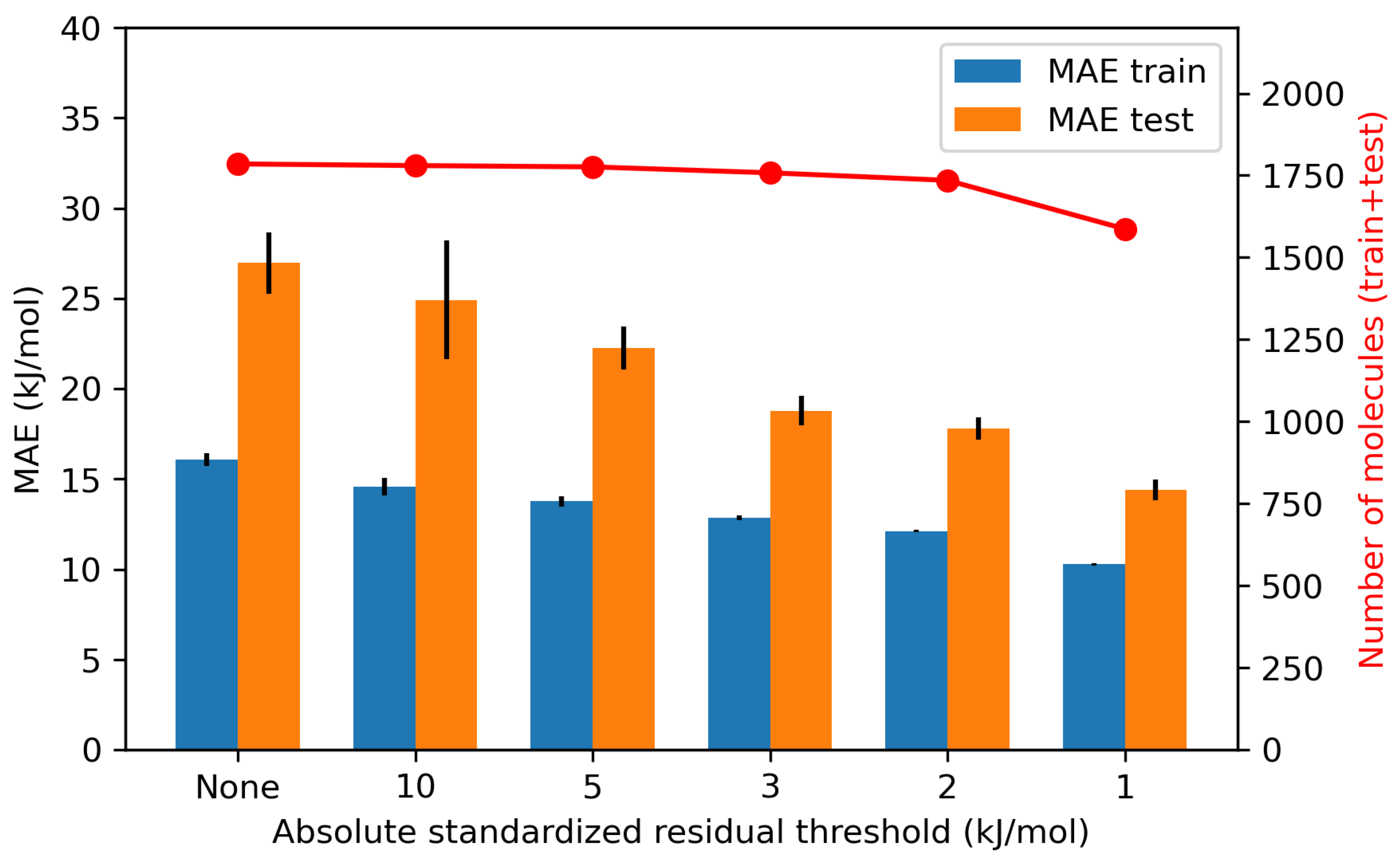
4.1.3. Effects of Model-Outliers on the Model Performance

The same procedure as in Section 4.1.2 applies here but, this time, outliers are removed on the basis of their standardized residual values (Model-outliers) instead of the anomaly scores (X-outliers). In this sense, different thresholds of standardized residuals are tested, namely 1, 2, 3, 5 and 10, in absolute values. This means that the molecules with absolute standardized residual values above 1, 2, 3, 5 and 10 are removed from the preprocessed data.
Initially, the same effect (i.e., points that are not outliers before the removal of molecules become ones after the removal) as presented in Section 4.1.2 can be observed concerning the “data-relative” character of an outlier. Figure 8b shows the new standardized residuals versus the new RF confidence anomaly scores after removal of the points with initial absolute standardized residual values above three (see Figure 8a), for the enthalpy. It can be observed again that some points have increased their absolute standardized residual values after the outlier removal (points in red in Figure 8a,b). These points, corresponding mostly to molecules from the families of silicon and inorganic compounds, become less represented (at least, in a consistent manner in terms of the enthalpy values) in the new dataset, after the elimination of the Model-outliers. Besides, the elimination of the outliers with absolute standardized residuals above three seems to have reduced the range of standardized residuals, but not that of the RF confidence anomaly scores.
The effect of the elimination of outliers, based on their standardized residual, on the enthalpy model performance is presented in Figure 9. The x-axis represents the tested thresholds, a threshold of k corresponding to the elimination of all the molecules with absolute standardized residuals above k. Similarly as for the elimination of X-outliers based on anomaly scores, the model seems to improve its performance with the elimination of outliers with high absolute standardized residuals, while overfitting is also reduced. At the same time, the number of eliminated molecules is not as dramatic as in the case of X-outliers, allowing a wider margin of selection of the final threshold value. In fact, it is seen that only the strictest threshold of 1 kJ/mol, among the tested ones, results in a significant elimination of about 200 molecules, for a decrease in the MAE that remains comparable to the rest of the tested thresholds.

4.1.4. Effects of X-outliers and Model-outliers on the Model Performance

Previously, the effects of outliers, identified either in terms of the anomaly scores (X-outliers) or the standardized residuals (Model-outliers), on the performance of the ML models were studied individually. In this section, both aspects are considered combined, with RF confidence for the X-outlier detection method. More precisely, starting from the preprocessed data, the three layouts described in Section 3.3 are compared, with thresholds of 2 kJ/mol and 150 kJ/mol, respectively, for the absolute standardized residual and the RF confidence anomaly score.
The results for enthalpy are shown in Figure 10. In particular, Figure 10a represents the whole preprocessed dataset, prior to any outlier elimination, while Figure 10b–d, correspond to the same data but with an additional step of outlier elimination, according to Layouts 1–3, respectively. It can be observed that each outlier elimination scenario enables to obtain a cloud of points that lies inside a more restricted window, with respect to the initial dataset, even if some points that were not outliers become outliers during the elimination process. In any case, the clouds of points obtained with the three layouts look similar. Their performance and amount of molecules are also close, as observed in Figure 11.
All three layouts enable us to drastically improve the performance of the model (more than when only X-outliers or Model-outliers are removed with the same thresholds), achieving an overall two-fold decrease in the test M A E . Among the three tested scenarios, a slightly better performance is obtained for Layout 3 ( M A E train = 9.51 kJ/mol vs. 10.43 for Layout 1 and 10.51 for Layout 2; M A E test = 11.88 kJ/mol vs. 13.48 for Layout 1 and 13.58 for Layout 2), but this comes at the cost of a marginally increased elimination of molecules, with respect to the other two layouts (1531 remaining molecules vs. 1591 for Layout 1 and 1603 for Layout 2). Due to its higher performance, Layout 3 is therefore chosen as the outlier elimination method for the rest of this article. Note that Figure 11 highlights this compromise between the size of the AD and the reliability of the predictions, as already discussed.
Layout 3 is also applied for the elimination of outliers for the entropy, but with different threshold values for X-outliers in view of a higher density of the cloud of points in a smaller region (see Figure 4). These thresholds are set to 50 J/mol/K and 2 J/mol/K for the RF confidence anomaly score and the standardized residual, respectively. The resulting data are shown in Figure 12 and result again in a two-fold reduction in the model test M A E , though it is slightly better for Layout 3 ( M A E train = 7.49 J/mol/K vs. 8.61 for Layout 1 and 8.8 for Layout 2; M A E test = 8.19 J/mol/K vs. 9.82 for Layout 1 and 10 for Layout 2).

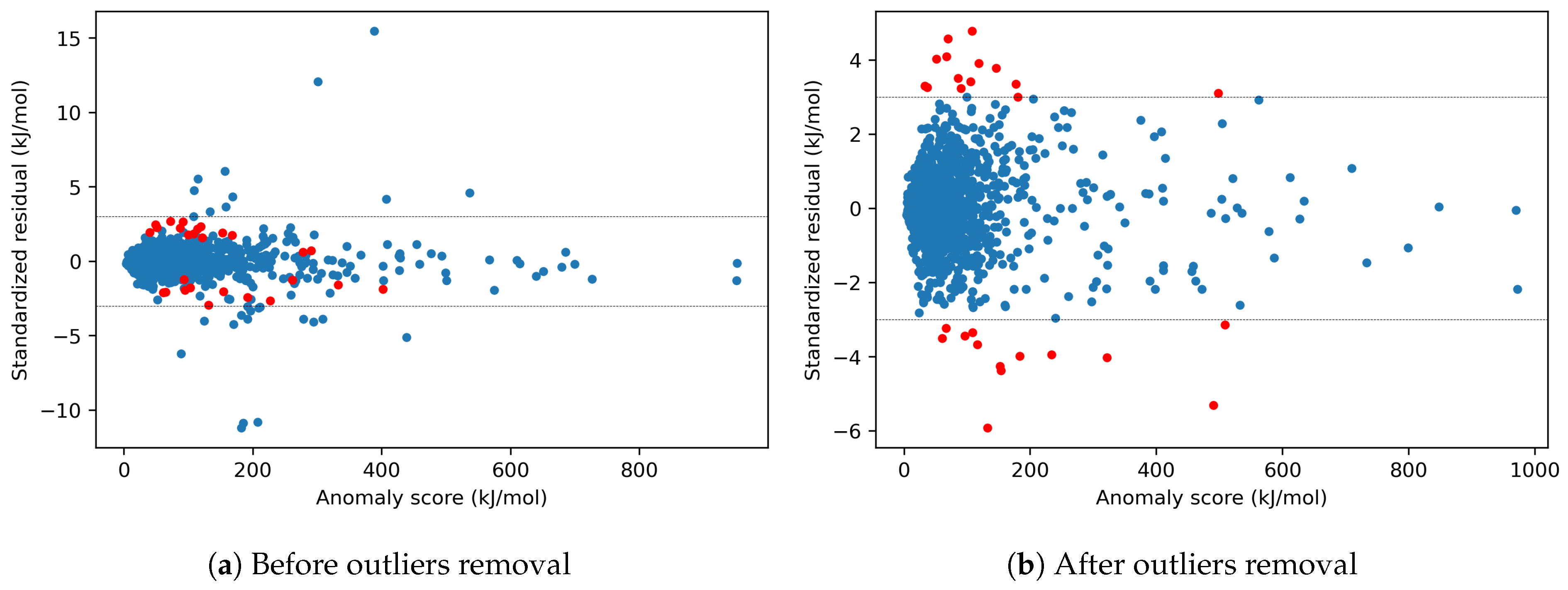
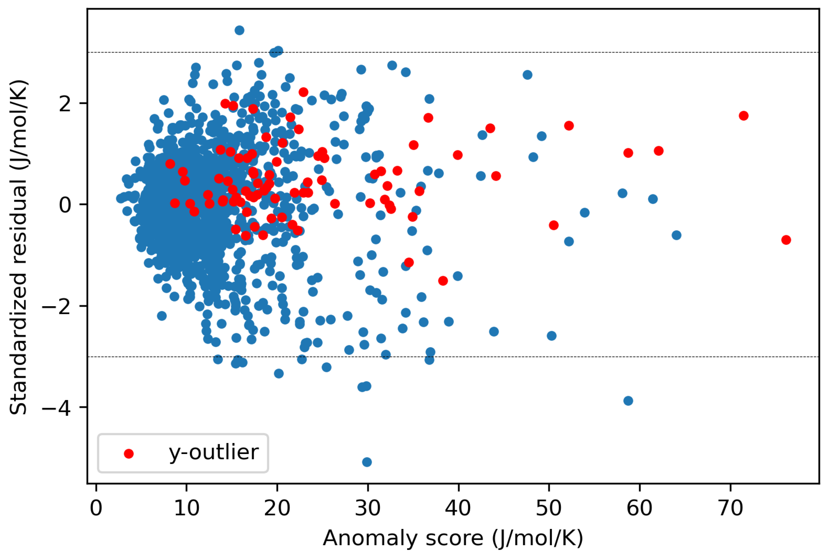
4.1.5. Effects of y-outliers on the Model Performance

Concerning the y-outliers still present in the dataset after the elimination of X-outliers and Model-outliers with Layout 3 (in red in Figure 10d and Figure 12), they were not eliminated, as this did not lead to a significant improvement in the performance of the models, as shown in Table 2. In fact, the removal of y-outliers does not necessarily improve the statistical parameters, since a y-outlier is not necessarily a Model-outlier. Indeed, Figure 10d and Figure 12 show that y-outliers have low standardized residuals. More generally, a y-outlier can have more or less impact on the overall model’s performance. If a molecule is both a y-outlier and a X-outlier, its thermodynamic property can be both well and poorly predicted: it will depend on if the ML model manages to extend its response surface to include this molecule. If a molecule is a y-outlier but not a X-outlier, this molecule represents a case of property cliff (i.e., similar structures but very different property values). In this case, the response surface can be pulled toward this molecule which can deteriorate the model’s performance in varying amounts. In this study, the model’s performance was improved for H after y-outliers removal, but not for S (cf. Table 2). It is difficult to qualitatively explain this difference between H and S, as the elimination of each individual y-outlier can have a positive or negative effect on the model’s performance. Accordingly, the overall trend can be different in each case. Finally, further elimination of X-outliers and/or Model-outliers would have been possible, allowing us to eventually further improve the performance of the models, but to the detriment of the loss of data and a further reduction in the size of the AD. In the end, it comes down to the user to select the most appropriate methods given the problem requirements and the available dataset characteristics.

4.2. AD Definition during ML Model Construction (Substudy 2)

4.2.1. Dimensionality Reduction on the Preprocessed Data without Outliers

To improve the interpretability of the models, a dimensionality reduction step based on GA is applied on the preprocessed data after outlier elimination through Layout 3. Note that the GA algorithm enables us to remove descriptors that are not relevant for the predicted property, while the elimination of X-outliers removes molecules that exhibit outlier behavior based on their descriptor values. The obtained performances are presented in Table 3 and Table 4 for the enthalpy and entropy, respectively, where configurations with or without outliers/dimensionality reduction are compared. The removal of the outliers enables us to improve the performance of the models (configurations A vs. B, and C vs. D), although the resulting AD might be restricted due to the elimination of some molecules. The dimensionality reduction does not seem to have a major impact on the performance (configurations A vs. C, and B vs. D), despite the significant reduction in the number of descriptors that are reduced from more than 2000 to only 100, thus enhancing the subsequent interpretability of the models.
In particular, for the enthalpy, with or without outlier elimination (configurations C and D), the 100 identified descriptors mostly belong to the following categories as defined by AlvaDesc: 2D atom pairs, atom-centered fragments and atom-type e-state indices. For the entropy, the most represented categories in the 100 identified descriptors, that seem to also depend on the outlier elimination step, are the following: 2D atom pairs, 2D autocorrelations and atom-centered fragments (instead of 2D atom pairs, functional group counts and CATS 3D descriptors when outliers are not eliminated). Note that the identified descriptors are fully detailed in the Supplementary Materials, as well as their corresponding coefficients in Lasso linear model. To better understand this variation for the entropy, Table A3 displays the most represented families in the eliminated outliers via Layout 3 for both enthalpy and entropy. For the entropy, the eliminated outliers seem to contain a large percentage of polyfunctional compounds and aromatics, not only as part of the respective individual families, but also as members of some other families, such as esters/ethers and nitrogen compounds (e.g., in esters/ethers, 50% are aromatic and 15% are polyfunctional). Therefore, their elimination could affect their relative importance, as described by the associated descriptors in the dataset. As for CATS 3D descriptors, they consider the spatial pairwise Euclidean distances between potential pharmacophore points or PPP (i.e., hydrogen-bond donor/acceptor, positive/negative, lipophilic) [63]. The elimination of esters/ethers, polyfunctional compounds, nitrogen compounds and aromatics, containing numerous PPP (e.g., the oxygen atom in an ester or ether group is a hydrogen-bond donor), reasonably affects the relevance of CATS 3D descriptors for the remaining data. More generally, these observations demonstrate that the dimensionality reduction step can be influenced by outliers, such as other processing steps. Accordingly, any eventual elimination of outliers should be performed early in the process, as is the case in this work. Other options include the deployment of specific methods that allow feature selection and outlier detection to be performed simultaneously, or robust regression or scaling in the presence of outliers [64,65,66,67,68,69,70,71,72,73].
Finally, configuration D seems to be a good compromise between model performance, interpretability and AD size. The parity plots obtained for this configuration are displayed in Figure 13 for the different train/test splits for enthalpy. The respective plots for entropy are shown in Figure A1. For both enthalpy and entropy, most molecules seem to be well predicted, despite some of them deviating from the main diagonal of the parity plots. This is mainly the case for test molecules and those displaying the highest prediction errors are highlighted in red with their identification numbers (ChemID) in Figure 13 and Figure A1.

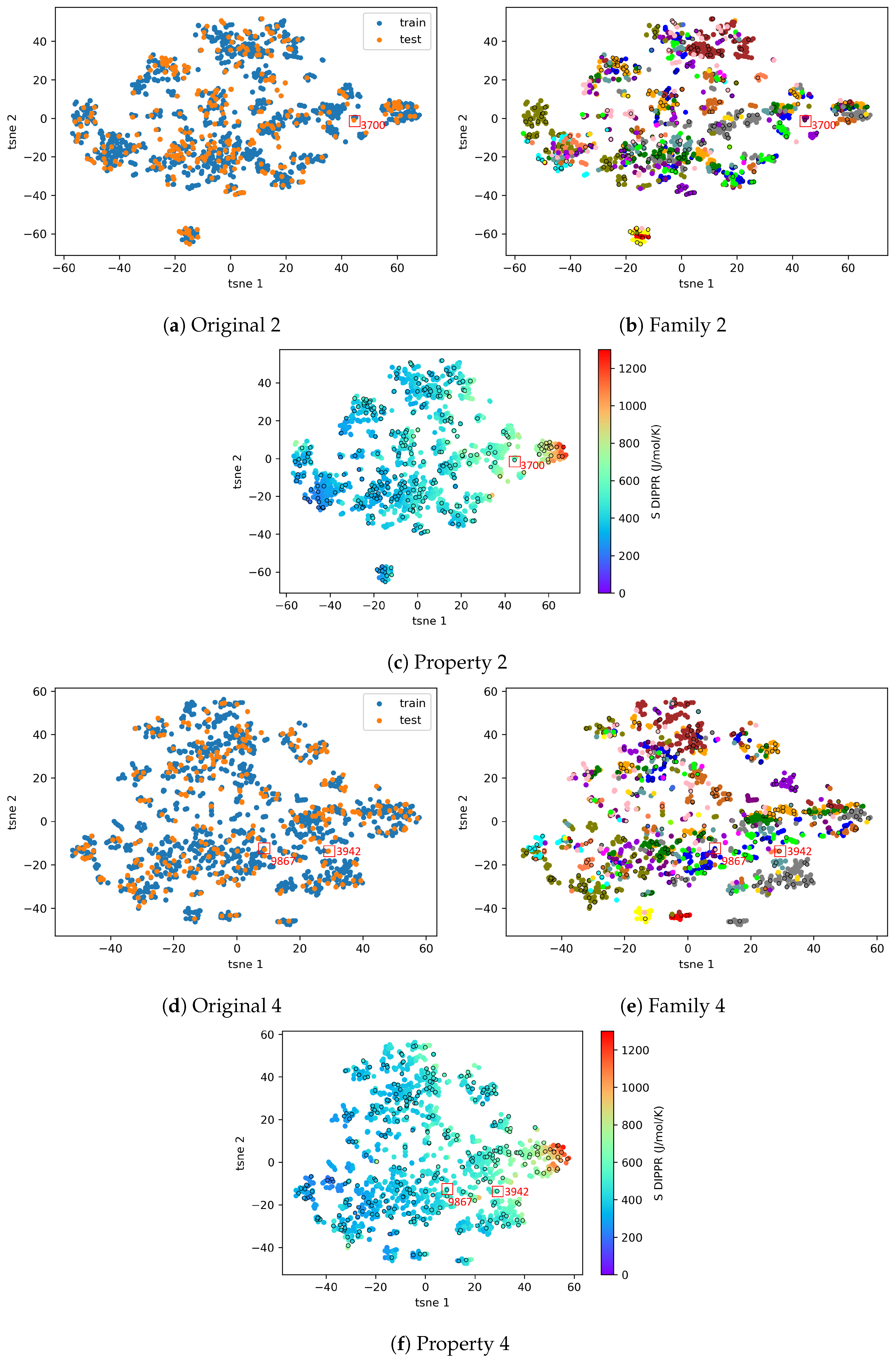
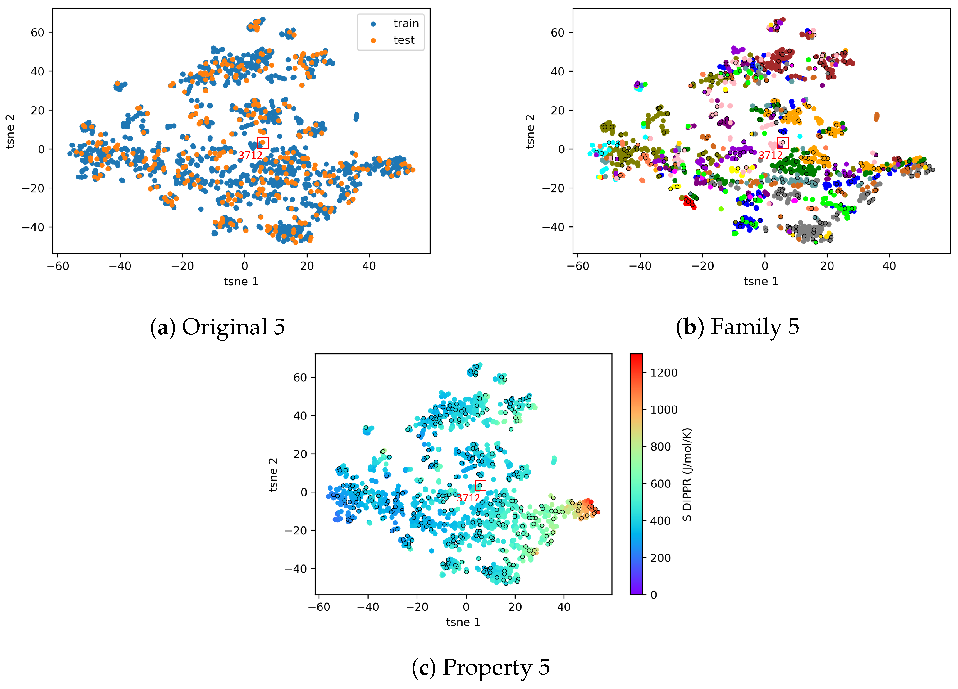
4.2.2. AD Visualization and Evaluation

One of the goals of this second substudy consists of visualizing where the test data are located with respect to the AD defined by the training data. In this sense, AD plots of Lasso standardized residuals versus RF confidence anomaly scores are presented in Figure 14 and Figure A2 for the enthalpy and entropy, respectively. These plots correspond to the same splits as the parity plots of Figure 13 and Figure A1. Most test data are located in low anomaly score regions (below 100–150 kJ/mol), similar to the training data. However, a paradox is observed for some points, belonging either to the train or test datasets, which, despite being located in high anomaly score areas, are well predicted by the model. At the same time, other points, located in intermediate anomaly score areas, display poorer predictions. This is, for example, the case for the test molecules with high prediction errors, previously highlighted in the parity plots, which all display intermediate anomaly scores. The origins of these higher prediction errors will be further investigated through tSNE 2D representations in the next part. More generally, the molecules with high standardized residuals are Model-outliers and their earlier elimination during the preprocessing step could be envisioned as a possible improvement, but under the risk that other molecules become Model-outliers (cf. data-related character of outlier as seen in substudy 1). Additionally, it seems that Model-outliers are more frequent in QSPR/QSAR studies that consider a wide diversity of structures [65], as is the case here, and therefore, building separate models for each category of molecules could also be envisioned, as suggested in the first article [15]. Indeed, the molecules highlighted in red in the parity plots and AD plots correspond to the following chemical families: inorganic, nitrogen, silicon and halogen compounds, and amines/amides. Some of these families were already present during the identification of Model-outliers during the preprocessing stage. This could be an indication that, for some specific families, the model is not able to describe the property value based on the selected descriptors.
As mentioned earlier, there is no known rule for the limits of the AD, especially regarding the considered method on the x-axis (on the y-axis, the same thresholds as in the leverage method could be considered). Examples of possible thresholds on the x-axis are the maximum anomaly value of training points or a value similar to the upper threshold in the IQR method. In both cases, it is clear that some test points are outside the AD (for x-axis) and should not be used for the model validation (except for testing the extrapolation capacity of the model). This was not further pursued in this work, as most test points were not concerned, but this is a possible improvement. In any case, the elimination of molecules decreases the possibilities of building a generic model.

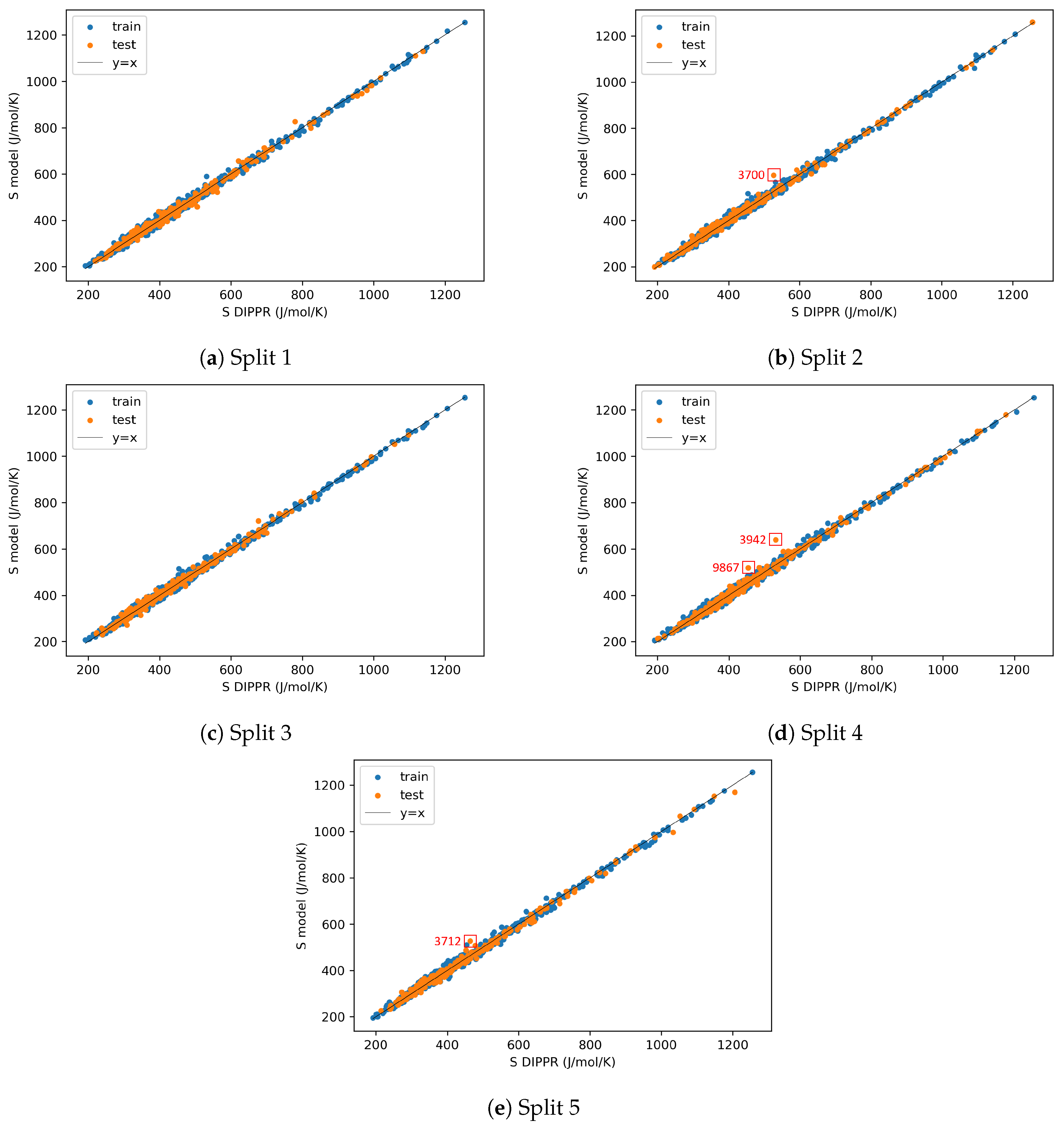
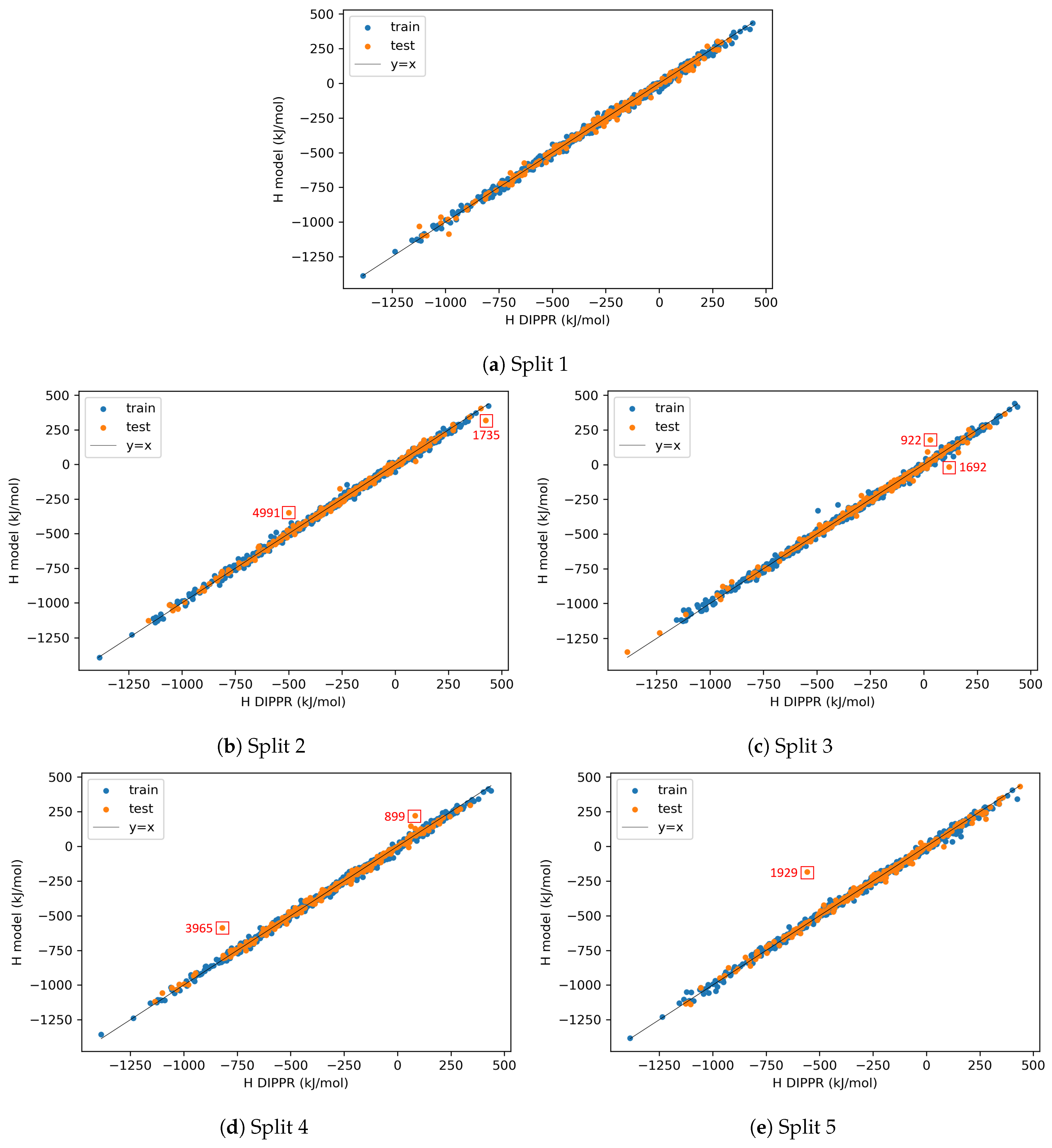
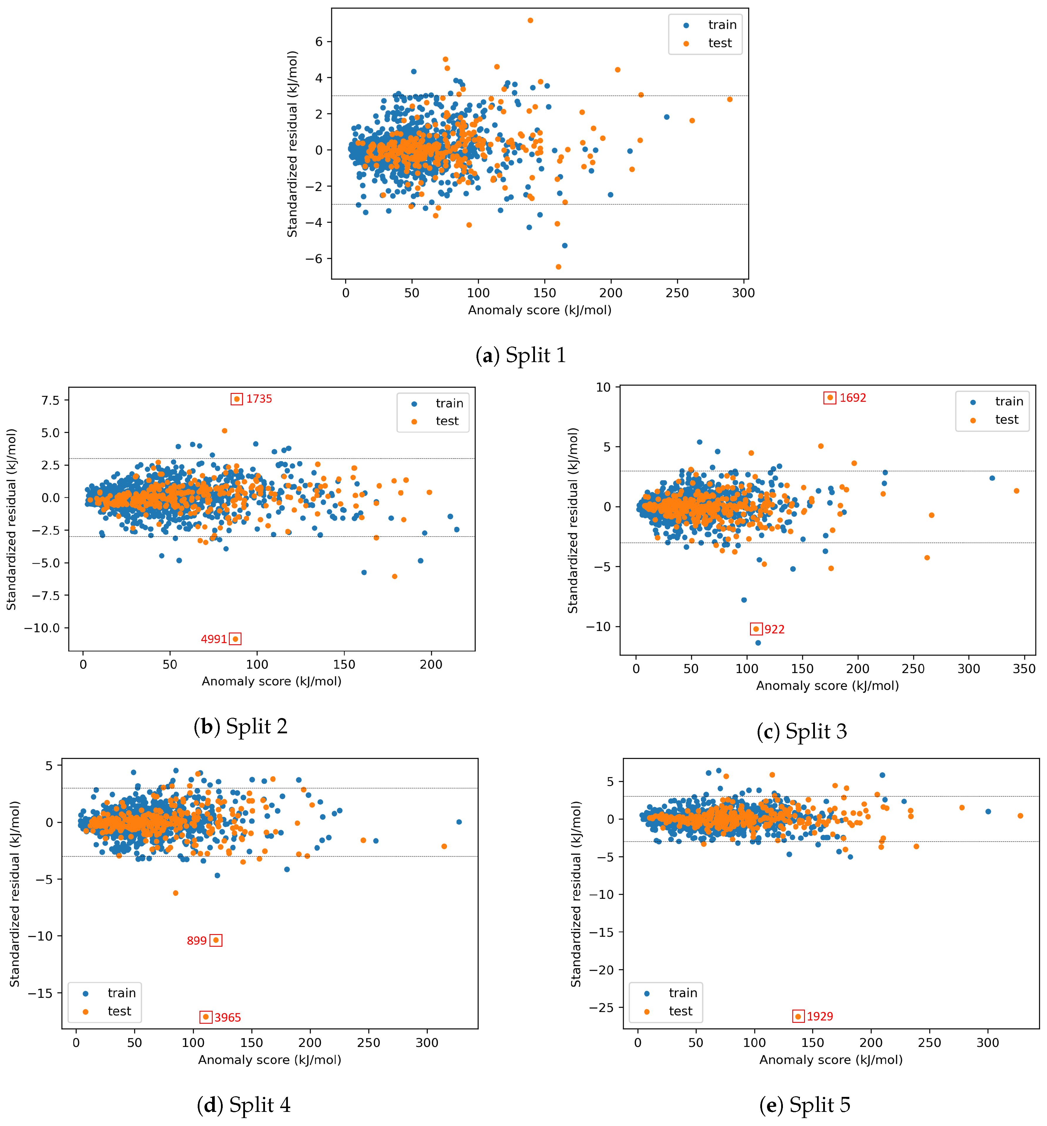
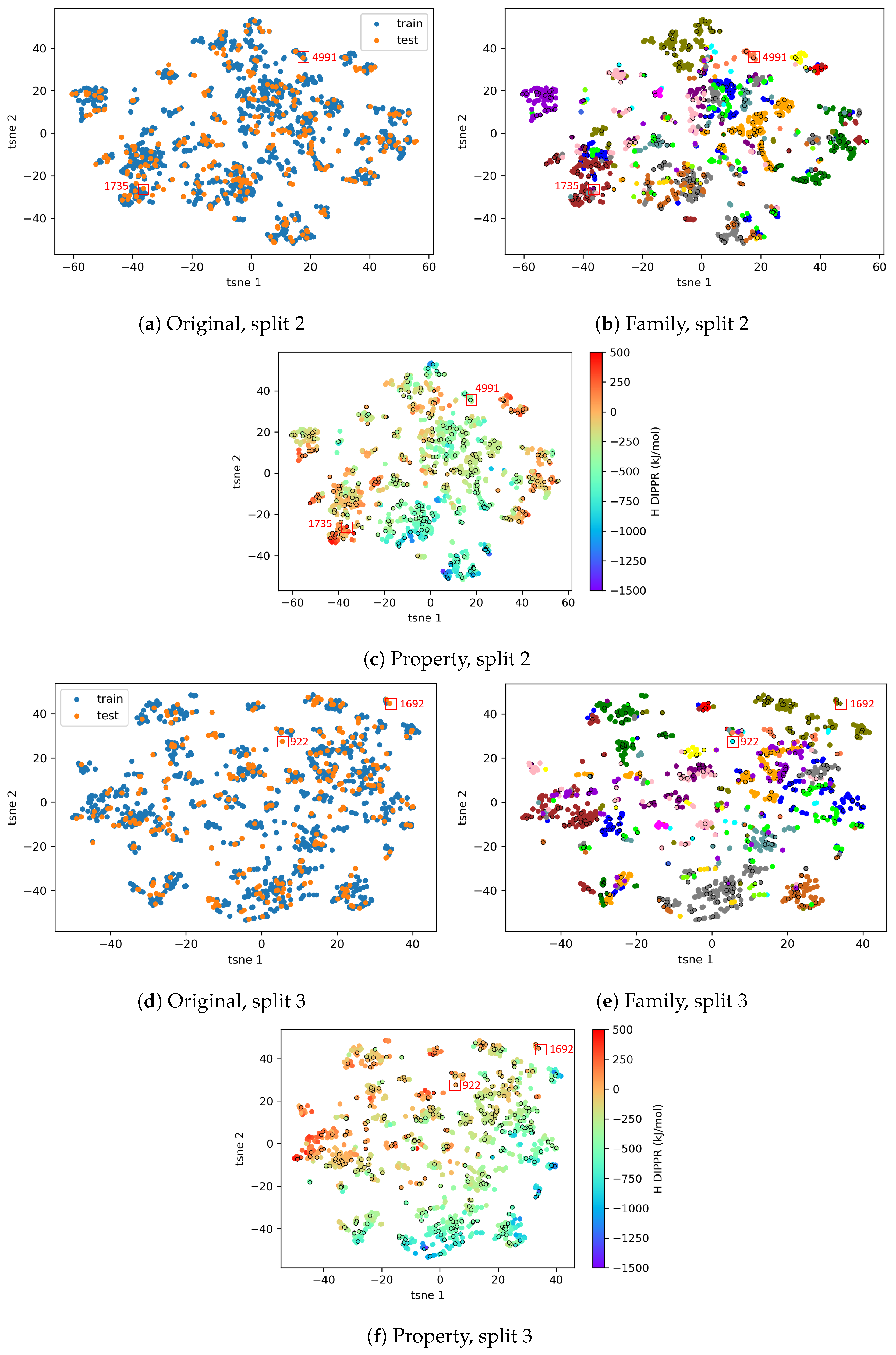
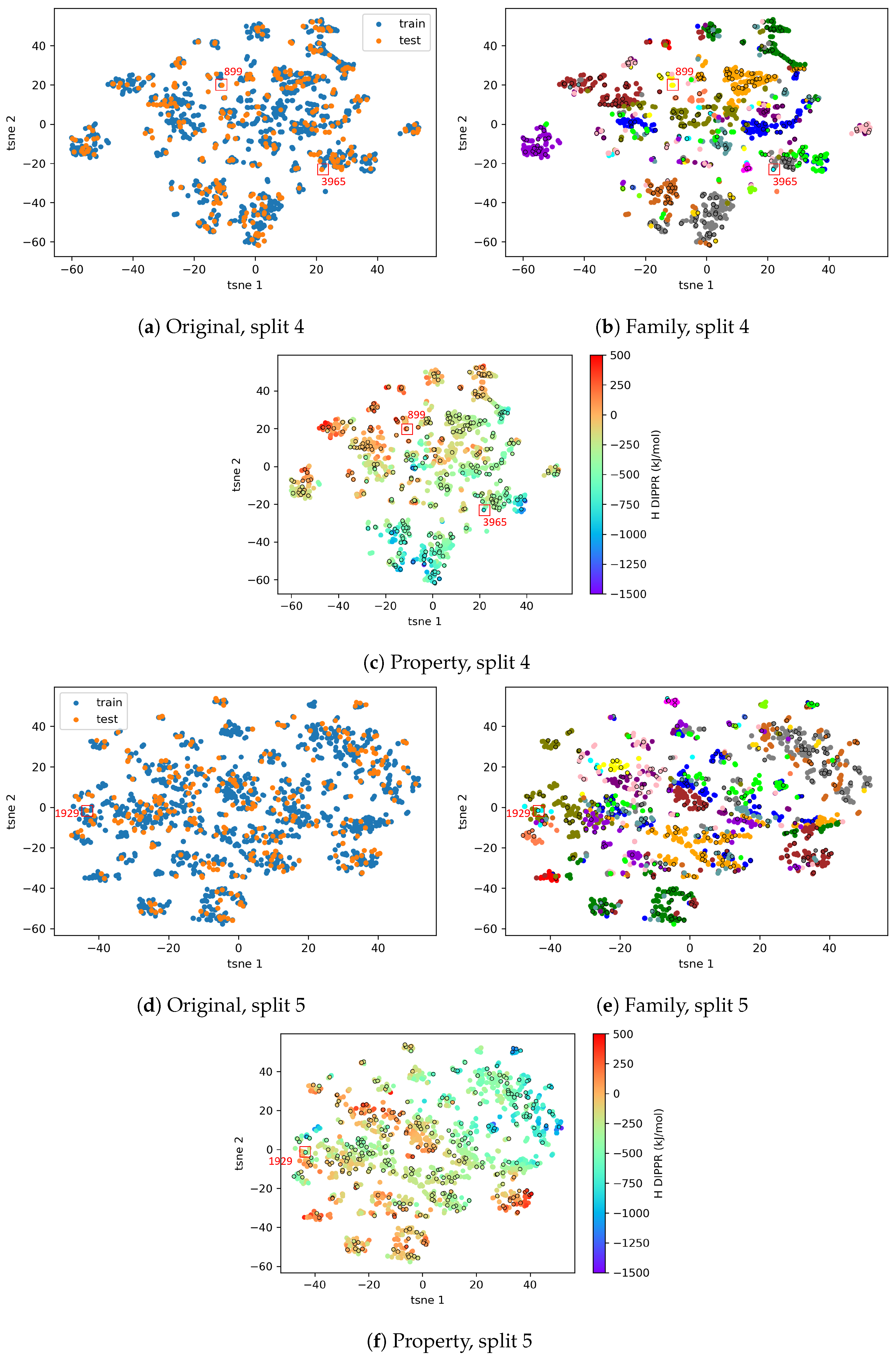
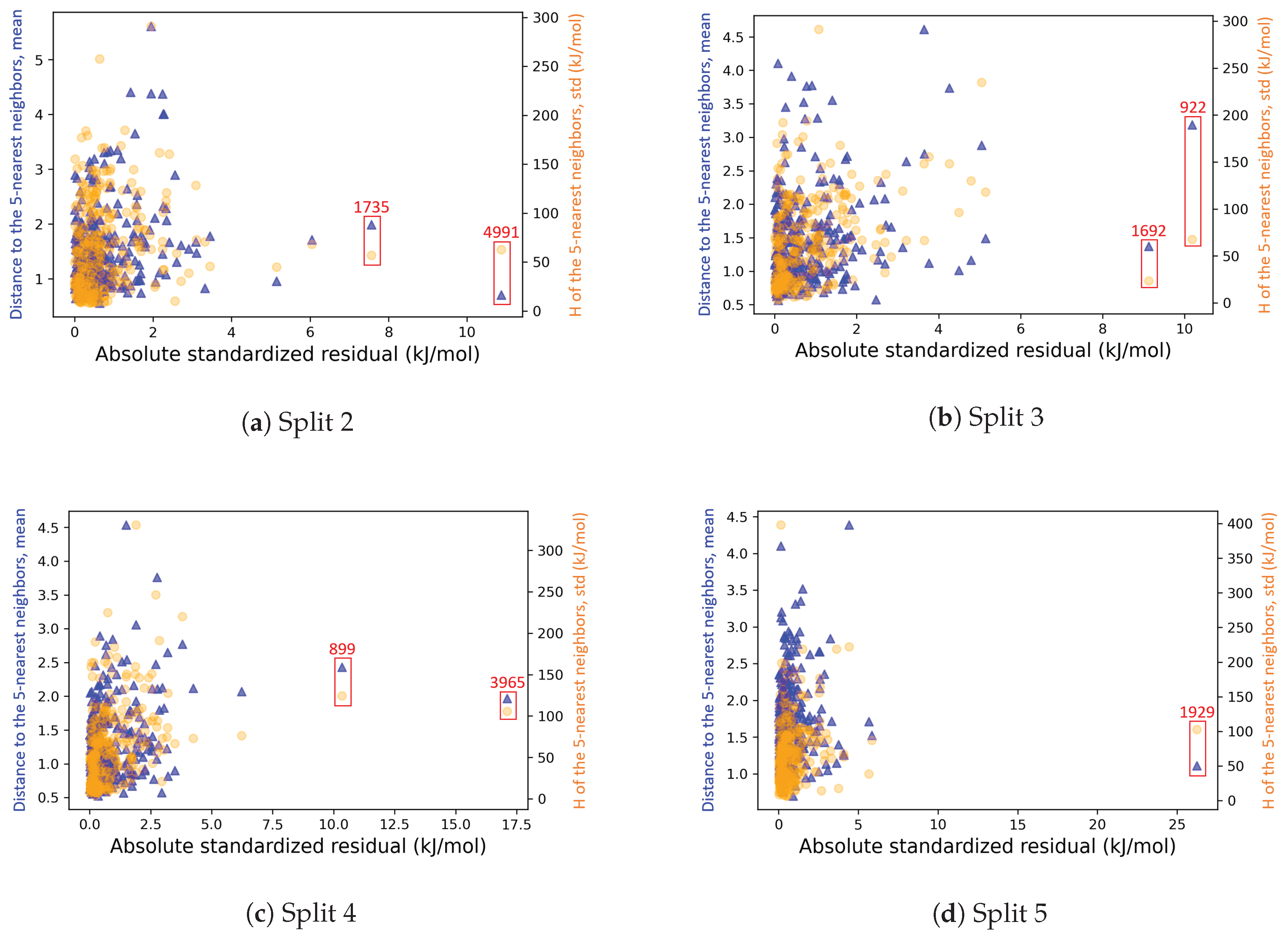
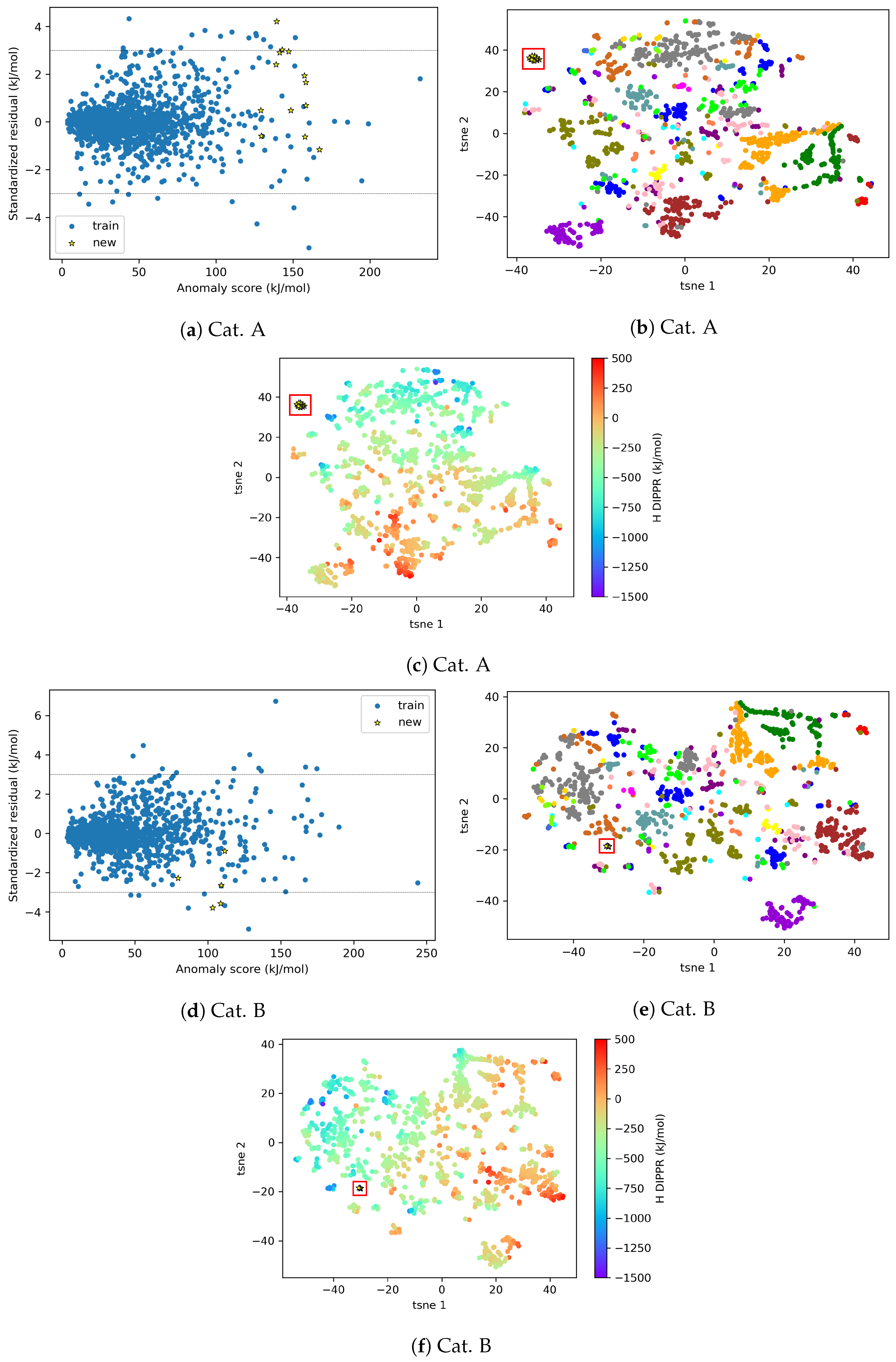
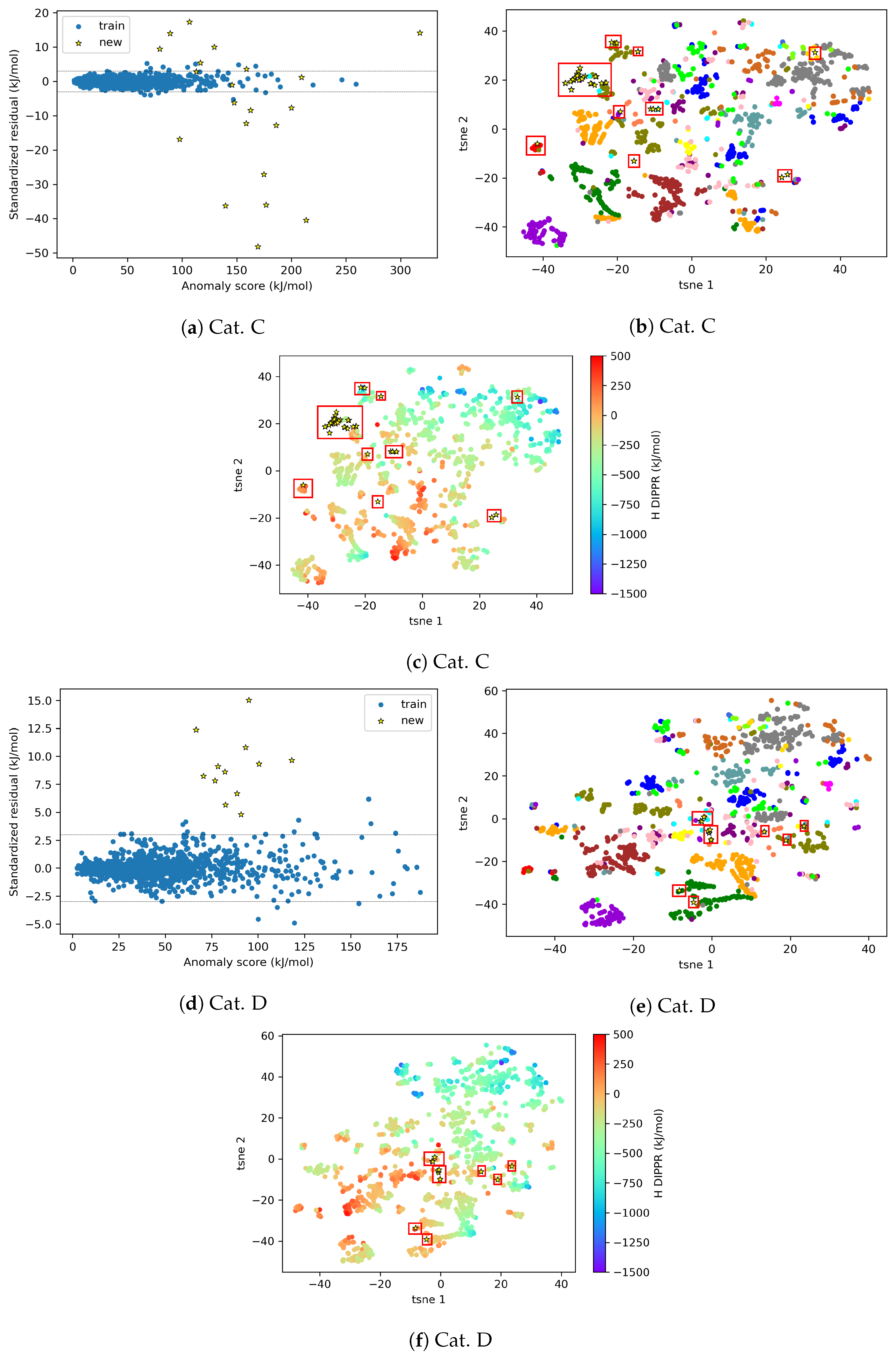
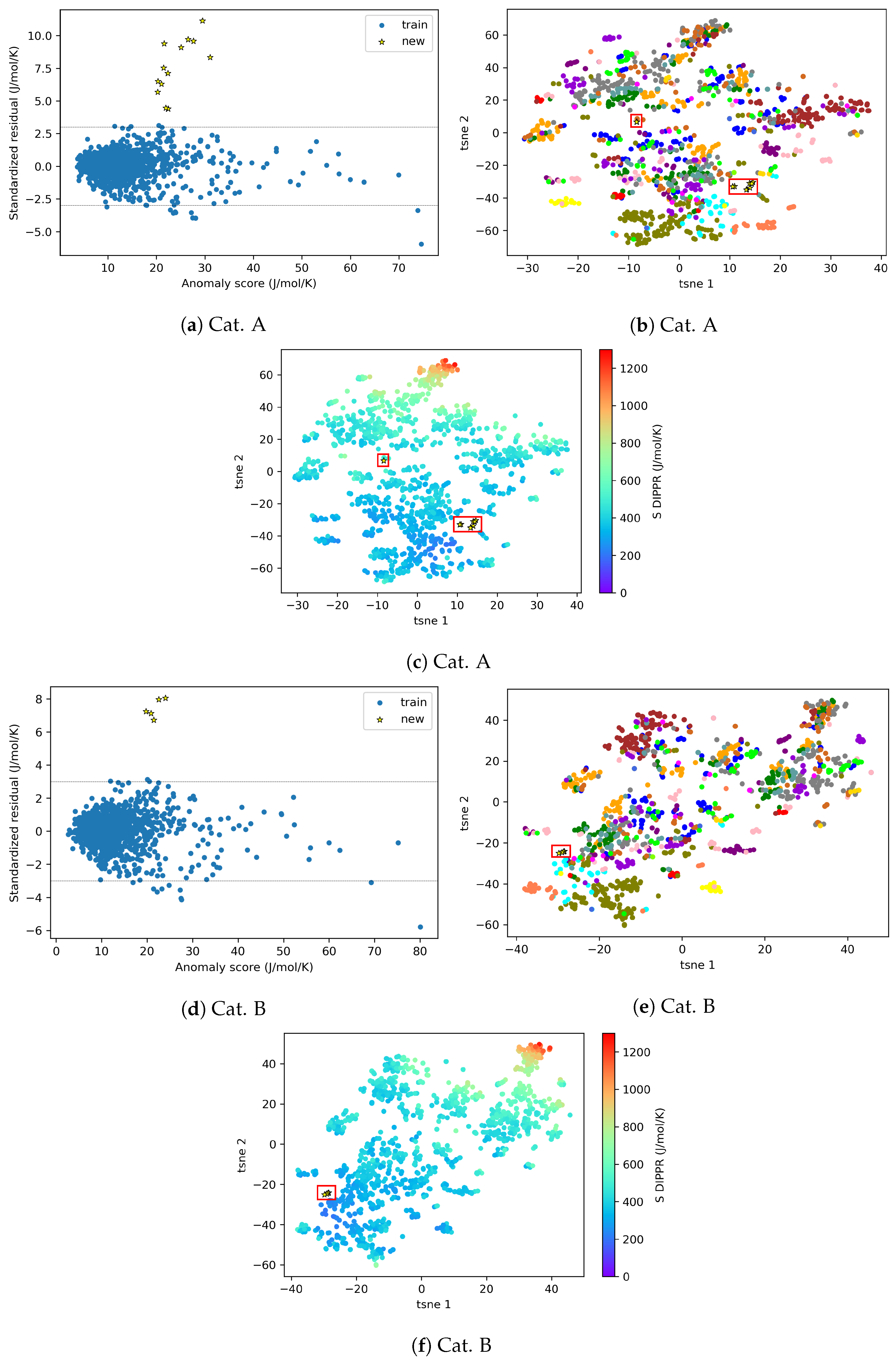
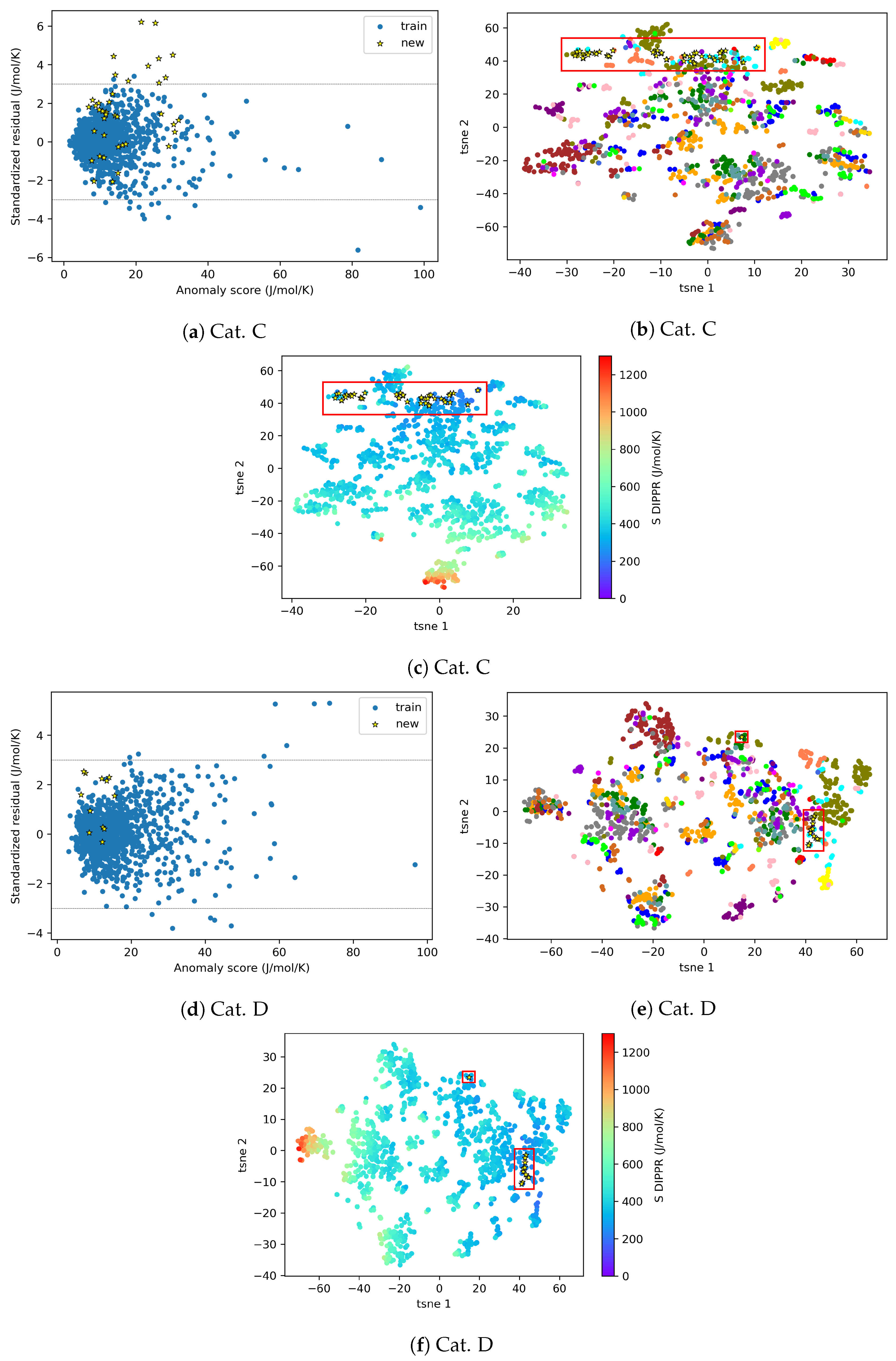
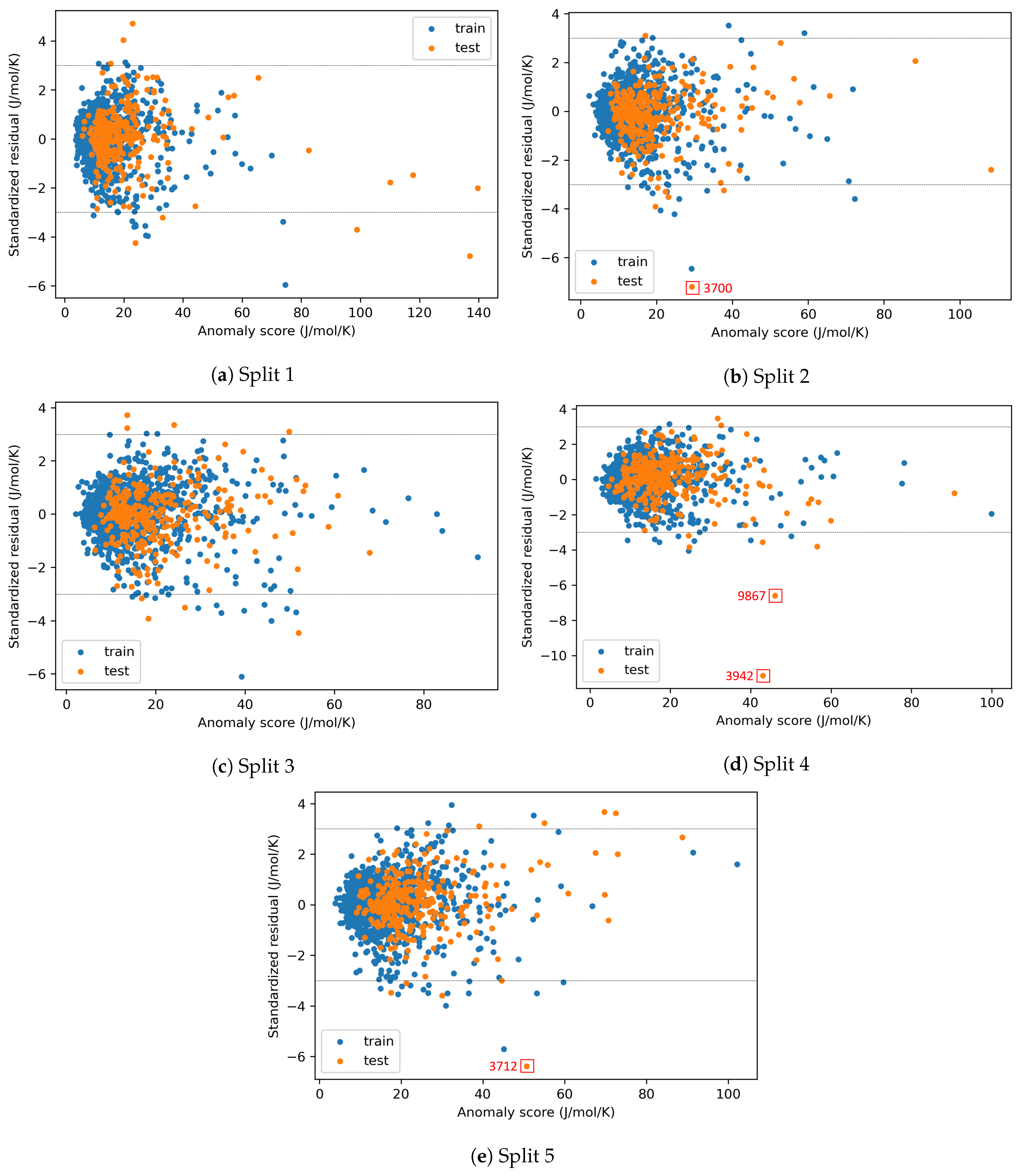
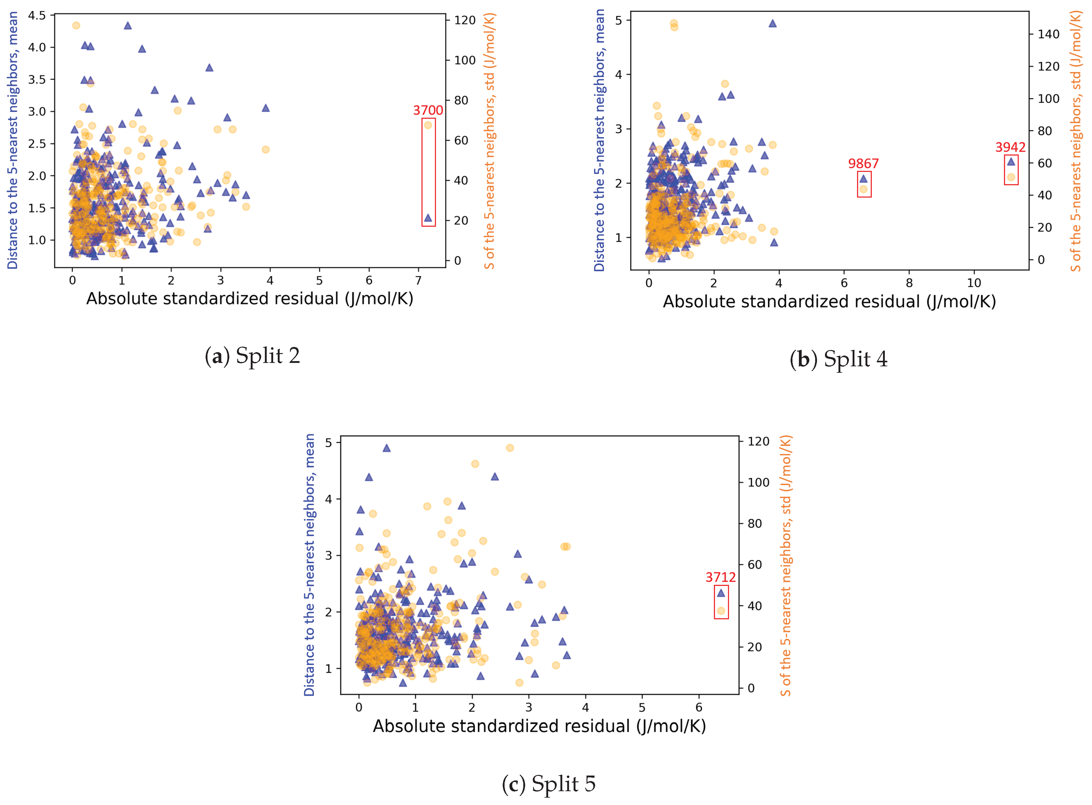
4.2.3. On the Understanding of the High Prediction Errors for Test Molecules

To provide further understanding of the high prediction errors of some test molecules, tSNE 2D is employed to visualize the data in a lower dimensional space. Figure 15a,d and Figure 16a,d correspond to the tSNE 2D representation of splits 2–5 for enthalpy. Figure 15b,e and Figure 16b,e reproduce the previously mentioned subfigures (Figure 15a,d and Figure 16a,d) but while highlighting a different distinctive characteristic of the plotted points. More specifically, these subfigures separate the molecules by chemical family, while those of Figure 15c,f and Figure 16c,f display the reference enthalpy values from the DIPPR database. In all the subfigures, the points with black contours correspond to the test data. The idea behind using all these representations is to find the source of high prediction errors for some test molecules. The hypotheses that are tested here are that these molecules are either located in a low-density area, in terms of the training descriptor space, or they are located in a high-density area but with a high variation in the training property values. Note that tSNE 2D representations of splits 2, 4 and 5 for the entropy are provided in Figure A3 and Figure A4. Also, for Figure 15b,e, Figure 16b,e, Figure A3b,e and Figure A4b, the color codes corresponding to different families are detailed in Figure A5.
First of all, it is noticeable that the tSNE 2D representation creates some clusters or regions which contain molecules of certain chemical families and/or have property values within a certain range. Indeed, the principle of tSNE is based on the conservation of the local structure of the data, meaning that similar data in a high-dimensional space will be plotted in a close vicinity in a lower-dimensional space. However, the region boundaries are not always clearly delimited and some points do not belong to clusters displaying the above characteristics. Several hypotheses could be put forward to explain this. First of all, the dimensional “compression” of a 100D space to a 2D one could be too high to allow for a clear data clustering. Another reason for the high diversity of chemical families that is observed in some of the formed clusters could be the fact that the selected descriptors (or even the use of molecular descriptors in general) leads to a classification of the molecules that is not completely consistent with their chemical classification in the established chemical families. In other words, molecules may be separated according to their similarities in terms of some descriptor values that would result in new families containing, for example, some alkanes and some esters. Finally, the shape of the clusters in tSNE representation is also highly dependent on the tSNE hyperparameter values, such as the perplexity, which is related to the number of nearest neighbors each point has [56,74].
Secondly, the combination of tSNE representations permits us to highlight the potential reasons for the observed high prediction errors of some test molecules. In this sense, one possible explanation—which is, for example, corroborated by the test molecules with the highest prediction errors in splits 4 and 5—is related to the isolation of these molecules from other “similar” ones in the training data. For example, in split 4, the molecules with chemid n°3965 and n°899, which are inorganic compounds, are close only to a few training molecules that are completely different in structure (i.e., esters/ethers and nitriles), thus displaying a significantly different property value. Another similar example concerns the amine molecule n°1735 and the inorganic molecule n°1929 in splits 2 and 5, which are located within a dense region composed of chemically diversified compounds (halogen and inorganic compounds for the first molecule; aromatics, epoxides and esters/ethers for the second one), which have large differences in property values.
Another possible explanation for the observed high prediction errors of some test molecules concerns molecules that are found completely isolated on the graphs, as a result of a low representation of their characteristics (i.e., as perceived by the model on the basis of the used descriptors) in the dataset. An example is the molecule n°922 in Split 3. Finally, it is also observed that some clusters are formed by molecules that display high variation in their enthalpy value, although the value is identified as “similar” by the model. This can lead to underfitting and poor prediction performance in these areas and can be due either to the uncertainties that might exist in the reference property values in the DIPPR database, or to the incapacity of the (selected) descriptors to capture the complete spectrum of structural differences of the molecules that are associated with the measured property. In this sense, different approaches exist in the literature where the use of descriptors is replaced by alternative molecular representation methods, such as graph neural networks (GNN), each one displaying its own advantages and drawbacks [75,76,77].
The fact that test molecules, having close training neighbors (in tSNE 2D projection) with low variance in their property values, are generally well predicted can be more clearly visualized in Figure 17. Here, again, the results shown are only for splits 2 to 5 for the enthalpy, but the results for splits 2, 4 and 5 for the entropy are also available in Figure A6. In particular, Figure 17 shows, for each test point, the average distance to its five nearest training neighbors and the standard deviation in the property values of these same neighbors, in relation to the prediction error of the test point. What is observable is that most points are located on the bottom-left corner, which confirms that well-predicted test points are generally those that have close training neighbors with low variance in their property values. However, a high distance to training points and/or a high variance in the property value of closest training points do not always lead to poor predictions, while, in some rare cases, molecules displaying relatively small distance to their five nearest neighbors and small standard deviation in the property values of these neighbors, are poorly predicted by the model. This is, for example, the case of the molecule n°4991 in Split 2 or the molecule n°1692 in Split 3. Further analyses are needed to better explain this contradicting behavior, but the previously emitted hypotheses can also apply here, including the unadapted descriptor-based representation, the imperfect tSNE 2D representation, the lack of training data in some regions, the AD representation ignoring the influence of the descriptors on the model, the presence of property cliffs, or the uncertainties in the DIPPR property values.

4.3. AD Definition during ML Model Deployment (Substudy 3)

In this last substudy, the objective is to show a concrete deployment of the developed ML-QSPR models to new species, including the predictions and the analysis of the reliability of the predictions with respect to the AD. As mentioned earlier, the new species are classified into four categories: A, B, C and D. It is necessary to divide the species into different categories to limit the loss of information. More concretely, one important limitation of descriptor-based approaches is their applicability when at least one descriptor cannot be calculated for the new query species. This is even more likely to happen with the models developed in this work, as they were trained on a large variety of chemical families and they are now being used to screen various types of species. Table 5 shows the number of descriptors that could not be calculated among the 100 selected by the GA method in each category of new species and each of the five train/test splits.
It can be observed that, for some categories of species, the number of impossible-to-calculate descriptors becomes significant before the total number of considered descriptors, reaching percentages in the order of 20% to 25%. This is, for example, the case for categories C and D, especially for the entropy calculation. Indeed, several species in these categories contain a specificity that prevents the calculation of several descriptors. Note that, in the DIPPR data that were used for the model construction, no species with this specificity were present. As such, the 100-GA descriptors, identified via the dimensionality reduction step, do not necessarily represent these species adequately. One possible solution would have been to develop a ML model based on data enriched with similar species as those in categories C and D; however, they were not readily available during the study. Another factor preventing the calculation of certain descriptor values for Cat. C species is also related to the presence of specific atoms [54]. In fact, a posterior analysis has revealed that the few molecules that exist in the DIPPR database, containing these specific atoms, were eliminated during the preprocessing stage, either due to missing property or descriptor values (cf. first article of the series [15]).
Consequently, the ML/QSPR models needed to be retrained on the basis of the proportion of the 100 descriptors, selected using the GA method, which could be calculated for the new species, before implementing the model for the prediction of their properties. This turned out to be problematic in the case of category C, as the significant elimination of descriptors resulted in duplicate molecules in the training set (i.e., molecules that could no longer be differentiated on the basis of the remaining descriptors).
The parity plots for Split 1 are presented in Figure 18 and Figure 19 for the enthalpy and entropy, respectively. In Figure 18c, it is interesting to observe that the points showing higher distances to the y = x line correspond to species containing atoms that were not represented in the training data, as discussed earlier. The detailed predictions of the enthalpy and entropy of all the new species, according to various splits, are provided in the Supplementary Materials. The prediction errors of the new species vary depending on the splits, meaning that some species are better predicted in some splits than in others. In an attempt to assess the reliability of the predictions with respect to the AD, different visualizations are once again attempted in Figure 20, Figure 21, Figure 22 and Figure 23. In particular, subfigures a and d of these figures display the standardized residuals vs. the RF confidence anomaly scores of the training molecules and the new species of Split 1, for the enthalpy and entropy, respectively. Only the new species belonging to Cat. D—and some to Cat. C, in the case of the entropy—seem to have very low RF confidence anomaly scores. Therefore, their predicted property values should have a high reliability, and this is effectively the case, as their standardized residuals are also very low. Note that in this work, the standardized residuals for the new species are available (except for some in Cat. C), but in real conditions, this would not have been the case.
Conversely, for the rest of the new species and/or for enthalpy, the RF confidence anomaly scores are higher and the standardized residuals fluctuate significantly. For example, both very low (e.g., Cat. A or B for enthalpy) and very high (e.g., Cat. C or D for enthalpy, Cat. A or B for entropy) values are observed for the standardized residuals. By highlighting the chemical families and the reference property values (Figure 20b,c,e,f, Figure 21b,c,e,f, Figure 22b,c,e,f and Figure 23b,c,e,f), similarly as in substudy 2, it is possible to observe that the new species that are not well predicted are those located in regions with no—or very few—training points, or those located in higher density regions but with very different property values. However, it remains difficult to understand why some species that have high anomaly scores and/or are isolated from the training data can be either very well predicted (e.g., Cat. A and B in the case of enthalpy) or not (e.g., Cat. A and B in the case of entropy). Further work needs to be conducted to better assess the reliability of the predictions for new species, as the RF confidence anomaly score seems not to be a sufficient criterion.

5. Conclusions and Perspectives

In this work, the applicability domain (AD) of machine learning (ML) models trained on high-dimensional data is investigated. The considered models are two ML models developed in a previous article for the prediction of the ideal gas enthalpy of formation and entropy of molecules based on their high-dimensional descriptors [15].
The AD is crucial, as it describes the space of chemical characteristics in which the model can make predictions with a given reliability. This work studies the AD definition of a ML model all along its development procedure: during data preprocessing, model construction and model deployment. Inside each of these steps, the AD definition fulfills a different function. Three AD definition methods, commonly used for outlier detection in high-dimensional problems, were compared: isolation forest (iForest), random forest prediction confidence (RF confidence) and k-nearest neighbors in the 2D projection of descriptor space obtained via t-distributed stochastic neighbor embedding (tSNE2D/kNN). These methods compute an anomaly score which can be used similarly to the distance metrics of classical AD definition methods. A molecule is inside the AD if its distance to the training domain (or anomaly score here) is below a given threshold. Due to the curse of dimensionality, classical AD definition methods are generally unsuitable for high-dimensional problems.
During data preprocessing, the three AD definition methods were used to identify outlier molecules and the effect of their removal was investigated. A more significant improvement in model performance could be observed when outliers identified with RF confidence were removed (e.g., for a removal of 30% of outliers, test MAE was divided by 2.5, 1.6 and 1.1 for RF confidence, iForest and tSNE2D/kNN, respectively). While these three methods identify X-outliers, the effect of other types of outliers, namely Model-outliers and y-outliers, was also investigated. In particular, the elimination of X-outliers followed by elimination of Model-outliers enabled us to divide M A E and R M S E by two and three, respectively, while reducing overfitting phenomenon. The elimination of y-outliers did not display significant improvement in the model performance.
During model construction, the AD serves to check how validation or test data are located in comparison with training data. All test data were close to training data according to the RF confidence method; however, some test data displayed high prediction errors and tSNE 2D representations were used to identify the possible causes (e.g., molecule with chemical information not well represented in training data).
Finally, the developed models were deployed to predict the thermodynamic properties of different categories of molecules. The results show that anomaly scores calculated using the RF confidence method are not sufficient to judge the reliability of a prediction for a new molecule. Indeed, some new molecules with low/high anomaly scores were poorly/well predicted. Further research needs to be conducted to identify more appropriate metrics, possibly in combination with the RF confidence method, to benefit from the information contained in each metric.
More generally, the AD definition should be better integrated into any QSPR/QSAR procedure for later use of the developed models.

Supplementary Materials

The following supporting information can be downloaded at: https://www.mdpi.com/article/10.3390/a16120573/s1, S1 (excel): Data, outliers and ML predictions.

Author Contributions

C.T.: literature review, conceptualization, methodology, data curation and modeling, writing (original draft preparation, review and editing). D.M.: supervision, methodology, writing (review and editing). S.L. and O.H.: data provision, molecular and thermodynamic analyses, generation of data for substudy 3, writing (review and editing). All authors have read and agreed to the published version of the manuscript.

Funding

This research was funded by MESRI (Ministère de l’Enseignement supérieur, de la Recherche et de l’Innovation), and by the Institute Carnot ICEEL (Grant: “Recyclage de Pneus par Intelligence Artificielle-RePnIA”), France.

Data Availability Statement

The authors do not have the permission to share the data from DIPPR; only some information about the descriptors and the predictions are available in the Supplementary Material (excel). The data of the new species used during model deployment cannot be published.

Conflicts of Interest

The authors declare no conflict of interest.

Abbreviations

The following abbreviations are used in this manuscript:
ADApplicability domain.
DIPPRDesign institute for physical properties.
DFTDensity functional theory.
HEnthalpy for ideal gas at 298.15 K and 1 bar.
IQRInterquartile range.
GAGenetic algorithm.
GNNGraph neural network.
GPGaussian processes.
iForestIsolation forest.
kNNk-nearest neighbors.
LassoLeast absolute shrinkage and selection operator.
M A E Mean absolute error.
MLMachine learning.
OECDOrganisation for economic co-operation and development.
PCsPrincipal components.
PCAPrincipal component analysis.
QSARQuantitative structure–activity relationship.
QSPRQuantitative structure–property relationship.
R 2 Coefficient of determination.
REACHRegistration, Evaluation, Authorization and Restriction of CHemicals.
RFRandom forest.
RF confidenceRandom forest prediction confidence.
R M S E Root mean square error.
SAbsolute entropy of ideal gas at 298.15 K and 1 bar.
tSNEt-distributed stochastic neighbor embedding.

Appendix A. Identification of Model-outliers and X-outliers in the Preprocessed Data for Enthalpy

Table A1. Top Model-outliers in the preprocessed data for enthalpy.
Absolute StandardizedChemidFamily
Residual r i
r i 10 3608Halogen Compounds
2628Halogen Compounds
3862Polyfunctional Compounds
7886Polyfunctional Compounds
7887Polyfunctional Compounds
5 r i < 10 1840Sulfur Compounds
2254Organic Acids
1950Inorganic Compounds
1969Silicon Compounds
3 r i < 5 2283Organic Acids
3931Silicon Compounds
3948Silicon Compounds
3929Silicon Compounds
4994Silicon Compounds
9858Organic Salts
2619Halogen Compounds
6851Other Compounds
2995Silicon Compounds
3991Silicon Compounds
3958Silicon Compounds
2370Esters/Ethers
2653Halogen Compounds
2877Polyfunctional Compounds
3974Silicon Compounds
3898Inorganic Compounds
6850Organic Compounds
9866Nitrogen Compounds
Table A2. Top 10 X-outliers in the preprocessed data for enthalpy.
iForestRF ConfidencetSNE2D/kNN
  Chemid Family Chemid Family Chemid Family
13933Silicon Compounds2624Halogen Compounds3977Silicon Compounds
23932Silicon Compounds3933Silicon Compounds1509Halogen Compounds
32624Halogen Compounds1627Halogen Compounds1866Halogen Compounds
43931Silicon Compounds1631Halogen Compounds9879Nitrogen Compounds
52991Silicon Compounds1626Halogen Compounds9877Nitrogen Compounds
61631Halogen Compounds3881Polyfunctional Compounds90Alkanes
73877Other Compounds1930Inorganic Compounds5878Organic Acids
82995Silicon Compounds1864Halogen Compounds1097Ketones/Aldehydes
93348Esters/Ethers3932Silicon Compounds3056Ketones/Aldehydes
101627Halogen Compounds834Alkanes7883Nitrogen Compounds

Appendix B. Most Represented Families in the Eliminated Outliers (Layout 3) for Enthalpy and Entropy

Table A3. Most represented families in the eliminated outliers (Layout 3) for enthalpy and entropy.
EnthalpyEntropy
Halogen Compounds24%Esters/Ethers20%
Silicon Compounds16%Silicon Compounds13%
Esters/Ethers10%Polyfunctional Compounds9%
Nitrogen Compounds9%Nitrogen Compounds9%
Inorganic Compounds7%Aromatics7%
Total66%Total58%

Appendix C. AD Definition for Entropy During Model Construction

Figure A1. Parity plots for entropy after outlier elimination (Layout 3) and dimensionality reduction (GA).
Algorithms 16 00573 g0a1
Figure A2. Visualization of the AD for entropy after outlier elimination (Layout 3) and dimensionality reduction (GA).
Algorithms 16 00573 g0a2
Figure A3. tSNE 2D representations for entropy after outlier elimination (Layout 3) and dimensionality reduction (GA), splits 2 and 4.
Algorithms 16 00573 g0a3
Figure A4. tSNE 2D representations for entropy after outlier elimination (Layout 3) and dimensionality reduction (GA), split 5.
Algorithms 16 00573 g0a4
Figure A5. Chemical families considered in Figure 15b,e, Figure 16b,e, Figure A3b,e and Figure A4b.
Algorithms 16 00573 g0a5
Figure A6. Analysis of the causes of the high prediction errors for entropy after outlier elimination (Layout 3) and dimensionality reduction (GA).
Algorithms 16 00573 g0a6

References

  1. Netzeva, T.I.; Worth, A.P.; Aldenberg, T.; Benigni, R.; Cronin, M.T.; Gramatica, P.; Jaworska, J.S.; Kahn, S.; Klopman, G.; Marchant, C.A.; et al. Current status of methods for defining the applicability domain of (quantitative) structure-activity relationships. ATLA Altern. Lab. Anim. 2005, 33, 155–173. [Google Scholar] [CrossRef]
  2. McCartney, M.; Haeringer, M.; Polifke, W. Comparison of Machine Learning Algorithms in the Interpolation and Extrapolation of Flame Describing Functions. J. Eng. Gas Turbines Power 2020, 142, 061009. [Google Scholar] [CrossRef]
  3. Cao, X.; Yousefzadeh, R. Extrapolation and AI transparency: Why machine learning models should reveal when they make decisions beyond their training. Big Data Soc. 2023, 10, 20539517231169731. [Google Scholar] [CrossRef]
  4. European Commission Environment Directorate General. Guidance Document on the Validation of (Quantitative)Structure-Activity Relationships [(Q)Sar] Models; OECD: Paris, France, 2014; pp. 1–154. [Google Scholar]
  5. Dearden, J.C.; Cronin, M.T.; Kaiser, K.L. How not to develop a quantitative structure-activity or structure-property relationship (QSAR/QSPR). SAR QSA Environ. Res. 2009, 20, 241–266. [Google Scholar] [CrossRef] [PubMed]
  6. Singh, M.M.; Smith, I.F.C. Extrapolation with machine learning based early-stage energy prediction models. In Proceedings of the 2023 European Conference on Computing in Construction and the 40th International CIB W78 Conference, Crete, Greece, 10–12 July 2023; Volume 4. [Google Scholar] [CrossRef]
  7. Muckley, E.S.; Saal, J.E.; Meredig, B.; Roper, C.S.; Martin, J.H. Interpretable models for extrapolation in scientific machine learning. Digit. Discov. 2023, 2, 1425–1435. [Google Scholar] [CrossRef]
  8. Hoaglin, D.C.; Kempthorne, P.J. Influential Observations, High Leverage Points, and Outliers in Linear Regression: Comment. Stat. Sci. 1986, 1, 408–412. [Google Scholar] [CrossRef]
  9. Aggarwal, C.C.; Yu, P.S. Outlier detection for high dimensional data. In Proceedings of the ACM SIGMOD International Conference on Management of Data, Santa Barbara, CA, USA, 21–24 May 2001; pp. 37–46. [Google Scholar] [CrossRef]
  10. Akoglu, L.; Tong, H.; Koutra, D. Graph based anomaly detection and description: A survey. Data Min. Knowl. Discov. 2015, 29, 626–688. [Google Scholar] [CrossRef]
  11. Souiden, I.; Omri, M.N.; Brahmi, Z. A survey of outlier detection in high dimensional data streams. Comput. Sci. Rev. 2022, 44, 100463. [Google Scholar] [CrossRef]
  12. Smiti, A. A critical overview of outlier detection methods. Comput. Sci. Rev. 2020, 38, 100306. [Google Scholar] [CrossRef]
  13. Cao, D.S.; Liang, Y.Z.; Xu, Q.S.; Li, H.D.; Chen, X. A New Strategy of Outlier Detection for QSAR/QSPR. J. Comput. Chem. 2010, 31, 592–602. [Google Scholar] [CrossRef]
  14. De Maesschalck, R.; Estienne, F.; Verdu-Andres, J.; Candolfi, A.; Centner, V.; Despagne, F.; Jouan-Rimbaud, D.; Walczak, B.; Massart, D.L.; De Jong, S.; et al. The development of calibration models for spectroscopic data using principal component regression [Review]. Internet J. Chem. 1999, 2, 1–21. [Google Scholar]
  15. Trinh, C.; Tbatou, Y.; Lasala, S.; Herbinet, O.; Meimaroglou, D. On the Development of Descriptor-Based Machine Learning Models for Thermodynamic Properties. Part 1—From Data Collection to Model Construction: Understanding of the Methods and their Effects. Processes 2023, 11, 3325. [Google Scholar] [CrossRef]
  16. Sahigara, F.; Mansouri, K.; Ballabio, D.; Mauri, A.; Consonni, V.; Todeschini, R. Comparison of different approaches to define the applicability domain of QSAR models. Molecules 2012, 17, 4791–4810. [Google Scholar] [CrossRef] [PubMed]
  17. Jaworska, J.; Nikolova-Jeliazkova, N.; Aldenberg, T. QSAR applicability domain estimation by projection of the training set in descriptor space: A review. ATLA Altern. Lab. Anim. 2005, 33, 445–459. [Google Scholar] [CrossRef] [PubMed]
  18. Mathea, M.; Klingspohn, W.; Baumann, K. Chemoinformatic Classification Methods and their Applicability Domain. Mol. Inform. 2016, 35, 160–180. [Google Scholar] [CrossRef] [PubMed]
  19. Roy, K.; Kar, S.; Ambure, P. On a simple approach for determining applicability domain of QSAR models. Chemom. Intell. Lab. Syst. 2015, 145, 22–29. [Google Scholar] [CrossRef]
  20. Yalamanchi, K.K.; van Oudenhoven, V.C.; Tutino, F.; Monge-Palacios, M.; Alshehri, A.; Gao, X.; Sarathy, S.M. Machine Learning to Predict Standard Enthalpy of Formation of Hydrocarbons. J. Phys. Chem. A 2019, 123, 8305–8313. [Google Scholar] [CrossRef]
  21. Yalamanchi, K.K.; Monge-Palacios, M.; van Oudenhoven, V.C.; Gao, X.; Sarathy, S.M. Data Science Approach to Estimate Enthalpy of Formation of Cyclic Hydrocarbons. J. Phys. Chem. A 2020, 124, 6270–6276. [Google Scholar] [CrossRef]
  22. Aldosari, M.N.; Yalamanchi, K.K.; Gao, X.; Sarathy, S.M. Predicting entropy and heat capacity of hydrocarbons using machine learning. Energy AI 2021, 4, 100054. [Google Scholar] [CrossRef]
  23. Aouichaoui, A.R.; Fan, F.; Abildskov, J.; Sin, G. Application of interpretable group-embedded graph neural networks for pure compound properties. Comput. Chem. Eng. 2023, 176, 108291. [Google Scholar] [CrossRef]
  24. Balestriero, R.; Pesenti, J.; LeCun, Y. Learning in High Dimension Always Amounts to Extrapolation. arXiv 2021, arXiv:2110.09485. [Google Scholar]
  25. Ghorbani, H. Mahalanobis Distance and Its Application for detecting multivariate outliers. Ser. Math. Inform. 2019, 34, 583–595. [Google Scholar] [CrossRef]
  26. De Maesschalck, R.; Jouan-Rimbaud, D.; Massart, D.L. The Mahalanobis distance. Chemom. Intell. Lab. Syst. 2000, 50, 1–18. [Google Scholar] [CrossRef]
  27. Aouichaoui, A.R.; Fan, F.; Mansouri, S.S.; Abildskov, J.; Sin, G. Combining Group-Contribution Concept and Graph Neural Networks Toward Interpretable Molecular Property Models. J. Chem. Inf. Model. 2023, 63, 725–744. [Google Scholar] [CrossRef] [PubMed]
  28. Mauri, A.; Bertola, M. Alvascience: A New Software Suite for the QSAR Workflow Applied to the Blood–Brain Barrier Permeability. Int. J. Mol. Sci. 2022, 23, 12882. [Google Scholar] [CrossRef] [PubMed]
  29. Huoyu, R.; Zhiqiang, Z.; Zhanggao, L.; Zhenzhen, X. Quantitative structure–property relationship for the critical temperature of saturated monobasic ketones, aldehydes, and ethers with molecular descriptors. Int. J. Quantum Chem. 2022, 122, 1–10. [Google Scholar] [CrossRef]
  30. Cao, L.; Zhu, P.; Zhao, Y.; Zhao, J. Using machine learning and quantum chemistry descriptors to predict the toxicity of ionic liquids. J. Hazard. Mater. 2018, 352, 17–26. [Google Scholar] [CrossRef]
  31. Yousefinejad, S.; Mahboubifar, M.; Eskandari, R. Quantitative structure-activity relationship to predict the anti-malarial activity in a set of new imidazolopiperazines based on artificial neural networks. Malar. J. 2019, 18, 1–17. [Google Scholar] [CrossRef]
  32. Asadollahi, T.; Dadfarnia, S.; Shabani, A.M.H.; Ghasemi, J.B.; Sarkhosh, M. QSAR models for cxcr2 receptor antagonists based on the genetic algorithm for data preprocessing prior to application of the pls linear regression method and design of the new compounds using in silico virtual screening. Molecules 2011, 16, 1928–1955. [Google Scholar] [CrossRef]
  33. Kim, M.G. Sources of High Leverage in Linear Regression Model. J. Appl. Math. Inform. 2004, 16, 509–513. [Google Scholar]
  34. Leys, C.; Klein, O.; Dominicy, Y.; Ley, C. Detecting multivariate outliers: Use a robust variant of the Mahalanobis distance. J. Exp. Soc. Psychol. 2018, 74, 150–156. [Google Scholar] [CrossRef]
  35. Gramatica, P. Principles of QSAR models validation: Internal and external. QSAR Comb. Sci. 2007, 26, 694–701. [Google Scholar] [CrossRef]
  36. Varamesh, A.; Hemmati-Sarapardeh, A.; Dabir, B.; Mohammadi, A.H. Development of robust generalized models for estimating the normal boiling points of pure chemical compounds. J. Mol. Liq. 2017, 242, 59–69. [Google Scholar] [CrossRef]
  37. Sabando, M.V.; Ponzoni, I.; Soto, A.J. Neural-based approaches to overcome feature selection and applicability domain in drug-related property prediction. Appl. Soft Comput. J. 2019, 85, 105777. [Google Scholar] [CrossRef]
  38. Huang, J.; Fan, X. Reliably assessing prediction reliability for high dimensional QSAR data. Mol. Divers. 2013, 17, 63–73. [Google Scholar] [CrossRef] [PubMed]
  39. Rakhimbekova, A.; Madzhidov, T.; Nugmanov, R.I.; Baskin, I.; Varnek, A.; Rakhimbekova, A.; Madzhidov, T.; Nugmanov, R.I.; Gimadiev, T.; Baskin, I. Comprehensive Analysis of Applicability Domains of QSPR Models for Chemical Reactions. Int. J. Mol. Sci. 2021, 21, 5542. [Google Scholar] [CrossRef] [PubMed]
  40. Kaneko, H.; Funatsu, K. Applicability domain based on ensemble learning in classification and regression analyses. J. Chem. Inf. Model. 2014, 54, 2469–2482. [Google Scholar] [CrossRef]
  41. Rasmussen, C.E.; Williams, C.K.I. Gaussian Processes for Machine Learning; MIT Press: Cambridge, MA, USA, 2006. [Google Scholar]
  42. Sushko, I. Applicability Domain of QSAR Models. Ph.D. Thesis, Technical University of Munich, Munich, Germany, 2011. [Google Scholar]
  43. Kamalov, F.; Leung, H.H. Outlier Detection in High Dimensional Data. J. Inf. Knowl. Manag. 2020, 19, 1–15. [Google Scholar] [CrossRef]
  44. Riahi-Madvar, M.; Nasersharif, B.; Azirani, A.A. Subspace outlier detection in high dimensional data using ensemble of PCA-based subspaces. In Proceedings of the 26th International Computer Conference, Computer Society of Iran, CSICC 2021, Tehran, Iran, 3–4 March 2021. [Google Scholar] [CrossRef]
  45. Kriegel, H.P.; Kr, P.; Schubert, E.; Zimek, A. Outlier Detection in Axis-Parallel Subspaces of High Dimensional Data; Springer: Berlin Heidelberg, Germany, 2009; Volume 1, pp. 831–838. [Google Scholar]
  46. Filzmoser, P.; Maronna, R.; Werner, M. Outlier identification in high dimensions. Comput. Stat. Data Anal. 2008, 52, 1694–1711. [Google Scholar] [CrossRef]
  47. Angiulli, F.; Pizzuti, C. Fast outlier detection in high dimensional spaces. In Proceedings of the Principles of Data Mining and Knowledge Discovery, 6th European Conference PKDD, Helsinki, Finland, 19–23 August 2002; pp. 29–41. [Google Scholar]
  48. Kriegel, H.P.; Schubert, M.; Zimek, A. Angle-based outlier detection in high-dimensional data. In Proceedings of the ACM SIGKDD International Conference on Knowledge Discovery and Data Mining, Las Vegas, NV, USA, 24–27 August 2008; pp. 444–452. [Google Scholar] [CrossRef]
  49. Liu, F.T.; Ting, K.M.; Zhou, Z.H. Isolation-based anomaly detection. ACM Trans. Knowl. Discov. Data 2012, 6, 1–39. [Google Scholar] [CrossRef]
  50. Thudumu, S.; Branch, P.; Jin, J.; Singh, J.J. A comprehensive survey of anomaly detection techniques for high dimensional big data. J. Big Data 2020, 7, 42. [Google Scholar] [CrossRef]
  51. Xu, X.; Liu, H.; Li, L.; Yao, M. A comparison of outlier detection techniques for high-dimensional data. Int. J. Comput. Intell. Syst. 2018, 11, 652–662. [Google Scholar] [CrossRef]
  52. Zimek, A.; Schubert, E.; Kriegel, H.P. A survey on unsupervised outlier detection in high-dimensional numerical data. Stat. Anal. Data Min. 2012, 5, 363–387. [Google Scholar] [CrossRef]
  53. Erfani, S.M.; Rajasegarar, S.; Karunasekera, S.; Leckie, C. High-dimensional and large-scale anomaly detection using a linear one-class SVM with deep learning. Pattern Recognit. 2016, 58, 121–134. [Google Scholar] [CrossRef]
  54. Alvascience, AlvaDesc (Software for Molecular Descriptors Calculation), Version 2.0.8. 2021. Available online: https://www.alvascience.com (accessed on 1 January 2023).
  55. Mauri, A. alvaDesc: A tool to calculate and analyze molecular descriptors and fingerprints. Methods Pharmacol. Toxicol. 2020, 2, 801–820. [Google Scholar] [CrossRef]
  56. van der Maaten, L.; Hinton, G. Visualizing Data using t-SNE. J. Mach. Learn. Res. 2008, 9, 2579–2605. [Google Scholar]
  57. Gaussian, Inc. Gaussian 09; Gaussian, Inc.: Wallingford, CT, USA, 2010. [Google Scholar]
  58. Montgomery, J.A.; Frisch, M.J.; Ochterski, J.W.; Petersson, G.A. A complete basis set model chemistry. VI. Use of density functional geometries and frequencies. J. Chem. Phys. 1999, 110, 2822–2827. [Google Scholar] [CrossRef]
  59. Becke, A.D. Thermochemistry. III. The role of exact exchange. J. Chem. Phys. 1993, 98, 5648–5652. [Google Scholar] [CrossRef]
  60. Miyoshi, A. GPOP Software, Rev. 2022.01.20m1. Available online: http://akrmys.com/gpop/ (accessed on 1 January 2023).
  61. Non-Positive Definite Covariance Matrices. Available online: https://www.value-at-risk.net/non-positive-definite-covariance-matrices (accessed on 1 June 2023).
  62. Cruz-Monteagudo, M.; Medina-Franco, J.L.; Pérez-Castillo, Y.; Nicolotti, O.; Cordeiro, M.N.D.; Borges, F. Activity cliffs in drug discovery: Dr Jekyll or Mr Hyde? Drug Discov. Today 2014, 19, 1069–1080. [Google Scholar] [CrossRef]
  63. Fechner, U.; Franke, L.; Renner, S.; Schneider, P.; Schneider, G. Comparison of correlation vector methods for ligand-based similarity searching. J. -Comput.-Aided Mol. Des. 2003, 17, 687–698. [Google Scholar] [CrossRef]
  64. Pedregosa, F.; Varoquaux, G.; Gramfort, A.; Michel, V.; Thirion, B.; Grisel, O.; Blondel, M.; Prettenhofer, P.; Weiss, R.; Dubourg, V.; et al. Scikit-learn: Machine Learning in Python. J. Mach. Learn. Res. 2011, 12, 2825–2830. [Google Scholar]
  65. Cao, D.; Liang, Y.; Xu, Q.; Yun, Y.; Li, H. Toward better QSAR/QSPR modeling: Simultaneous outlier detection and variable selection using distribution of model features. J.-Comput.-Aided Mol. Des. 2011, 25, 67–80. [Google Scholar] [CrossRef] [PubMed]
  66. Insolia, L.; Kenney, A.; Chiaromonte, F.; Felici, G. Simultaneous feature selection and outlier detection with optimality guarantees. Biometrics 2022, 78, 1592–1603. [Google Scholar] [CrossRef] [PubMed]
  67. Menjoge, R.S.; Welsch, R.E. A diagnostic method for simultaneous feature selection and outlier identification in linear regression. Comput. Stat. Data Anal. 2010, 54, 3181–3193. [Google Scholar] [CrossRef]
  68. Kim, S.S.; Park, S.H.; Krzanowski, W.J. Simultaneous variable selection and outlier identification in linear regression using the mean-shift outlier model. J. Appl. Stat. 2008, 35, 283–291. [Google Scholar] [CrossRef]
  69. Jimenez, F.; Lucena-Sanchez, E.; Sanchez, G.; Sciavicco, G. Multi-Objective Evolutionary Simultaneous Feature Selection and Outlier Detection for Regression. IEEE Access 2021, 9, 135675–135688. [Google Scholar] [CrossRef]
  70. Park, J.S.; Park, C.G.; Lee, K.E. Simultaneous outlier detection and variable selection via difference-based regression model and stochastic search variable selection. Commun. Stat. Appl. Methods 2019, 26, 149–161. [Google Scholar] [CrossRef]
  71. Wiegand, P.; Pell, R.; Comas, E. Simultaneous variable selection and outlier detection using a robust genetic algorithm. Chemom. Intell. Lab. Syst. 2009, 98, 108–114. [Google Scholar] [CrossRef]
  72. Tolvi, J. Genetic algorithms for outlier detection and variable selection in linear regression models. Soft Comput. 2004, 8, 527–533. [Google Scholar] [CrossRef]
  73. Wen, M.; Deng, B.C.; Cao, D.S.; Yun, Y.H.; Yang, R.H.; Lu, H.M.; Liang, Y.Z. The model adaptive space shrinkage (MASS) approach: A new method for simultaneous variable selection and outlier detection based on model population analysis. Analyst 2016, 141, 5586–5597. [Google Scholar] [CrossRef]
  74. t-SNE: The Effect of Various Perplexity Values on the Shape. Available online: https://scikit-learn.org/stable/auto_examples/manifold/plot_t_sne_perplexity.html (accessed on 1 June 2023).
  75. Wu, Z.; Pan, S.; Chen, F.; Long, G.; Zhang, C.; Yu, P.S. A Comprehensive Survey on Graph Neural Networks. IEEE Trans. Neural Netw. Learn. Syst. 2021, 32, 4–24. [Google Scholar] [CrossRef] [PubMed]
  76. Xu, K.; Jegelka, S.; Hu, W.; Leskovec, J. How powerful are graph neural networks? In Proceedings of the 7th International Conference on Learning Representations, ICLR 2019, New Orleans, LA, USA, 6–9 May 2019; pp. 1–17. [Google Scholar]
  77. Jiang, D.; Wu, Z.; Hsieh, C.Y.; Chen, G.; Liao, B.; Wang, Z.; Shen, C.; Cao, D.; Wu, J.; Hou, T. Could graph neural networks learn better molecular representation for drug discovery? A comparison study of descriptor-based and graph-based models. J. Cheminform. 2021, 13, 1–23. [Google Scholar] [CrossRef] [PubMed]
Figure 1. Classical methods for AD definition: (a) chemical-based methods, (b) range-based and geometric methods, (c) distance-based methods/k-nearest neighbors, (d) probability distribution-based methods.
Algorithms 16 00573 g001
Figure 2. AD plot employed in this study. The anomaly score on the x-axis is computed via different methods: iForest, RF confidence or tSNE2D/kNN.
Algorithms 16 00573 g002
Figure 3. Comparison of three X-outlier detection methods on the preprocessed data for enthalpy: (a) iForest, (b) tSNE2D/kNN, (c) RF confidence, (d) RF confidence combined with H values. y-outliers are identified via the IQR method.
Algorithms 16 00573 g003
Figure 4. X-outlier detection on the preprocessed data with RF confidence for entropy.
Algorithms 16 00573 g004
Figure 5. Evolution of Lasso model performance in predicting the enthalpy under different proportions of X-outliers removed from the preprocessed data: (a) iForest, (b) RF confidence, (c) tSNE2D/kNN.
Algorithms 16 00573 g005
Figure 6. Comparison of Lasso model performance in predicting the enthalpy under different proportions of X-outliers removed from the preprocessed data via the three tested methods on the (a) train and (b) test datasets.
Algorithms 16 00573 g006
Figure 7. Comparison of the dataset (a) before and (b) after the removal of X-outliers via the RF confidence method for enthalpy (the molecules with anomaly scores above 200 kJ/mol in (a) are removed). In red, the molecules that were not outliers in (a) become outliers in (b).
Algorithms 16 00573 g007
Figure 8. Comparison of the dataset (a) before and (b) after the removal of Model-outliers for enthalpy (elimination of the molecules with absolute standardized residuals above 3 kJ/mol in (a)). In red, the molecules that were not outliers in (a) become outliers in (b).
Algorithms 16 00573 g008
Figure 9. Evolution of Lasso model performance in predicting the enthalpy under different thresholds for Model-outlier elimination in the preprocessed data.
Algorithms 16 00573 g009
Figure 10. Effect of different scenarios of outlier elimination on the data set of the enthalpy.
Algorithms 16 00573 g010
Figure 11. Effect of different scenarios of outlier elimination on Lasso model performance in predicting the enthalpy.
Algorithms 16 00573 g011
Figure 12. Data set after the elimination of outliers with Layout 3 for the entropy.
Algorithms 16 00573 g012
Figure 13. Parity plots for enthalpy after outlier elimination (Layout 3) and dimensionality reduction (GA).
Algorithms 16 00573 g013
Figure 14. Visualisation of the AD for enthalpy after outlier elimination (Layout 3) and dimensionality reduction (GA).
Algorithms 16 00573 g014
Figure 15. tSNE 2D representations for enthalpy after outlier elimination (Layout 3) and dimensionality reduction (GA), splits 2 and 3. Subfigures (a) and (d) show the original data, distinguishing train and test sets. Subfigures (b) and (e) show the same respective data, distinguishing chemical families (color codes given in Figure A5). Subfigures (c) and (f) show the same respective data, distinguishing the reference H values from the DIPPR.
Algorithms 16 00573 g015
Figure 16. tSNE 2D representations for enthalpy after outlier elimination (Layout 3) and dimensionality reduction (GA), splits 4 and 5. Subfigures (a) and (d) show the original data, distinguishing train and test sets. Subfigures (b) and (e) show the same respective data, distinguishing chemical families (color codes given in Figure A5). Subfigures (c) and (f) show the same respective data, distinguishing the reference H values from the DIPPR.
Algorithms 16 00573 g016
Figure 17. Analysis of the causes of the high prediction errors for enthalpy after outlier elimination (Layout 3) and dimensionality reduction (GA).
Algorithms 16 00573 g017
Figure 18. Parity plots of the training molecules and the new species for enthalpy for Split 1.
Algorithms 16 00573 g018
Figure 19. Parity plots of the training molecules and new species for entropy for Split 1.
Algorithms 16 00573 g019
Figure 20. Visualization of the new species in Cat. A and B with respect to the AD of the enthalpy model for Split 1. Subfigures (a) and (d) show the standardized residuals vs. the RF confidence anomaly scores, distinguishing training data and new species. The other subfigures show the tSNE 2D representation of the same data, distinguishing chemical families (color codes given in Figure A5) for subfigures (b) and (e), or distinguishing the reference H values for subfigures (c) and (f).
Algorithms 16 00573 g020
Figure 21. Visualization of the new species in Cat. C and D with respect to the AD of the enthalpy model for Split 1. Subfigures (a) and (d) show the standardized residuals vs. the RF confidence anomaly scores, distinguishing training data and new species. The other subfigures show the tSNE 2D representation of the same data, distinguishing chemical families (color codes given in Figure A5) for subfigures (b) and (e), or distinguishing the reference H values for subplots (c) and (f).
Algorithms 16 00573 g021
Figure 22. Visualization of the new species in Cat. A and B with respect to the AD of the entropy model for Split 1. Subfigures (a) and (d) show the standardized residuals vs. the RF confidence anomaly scores, distinguishing training data and new species. The other subfigures show the tSNE 2D representation of the same data, distinguishing chemical families (color codes given in Figure A5) for subfigures (b) and (e), or distinguishing the reference S values for subfigures (c) and (f).
Algorithms 16 00573 g022
Figure 23. Visualization of the new species in Cat. C and D with respect to the AD of the entropy model for Split 1. Subfigures (a) and (d) show the standardized residuals vs. the RF confidence anomaly scores, distinguishing training data and new species. The other subplots show the tSNE 2D representation of the same data, distinguishing chemical families (color codes given in Figure A5) for subplots (b) and (e), or distinguishing the reference S values for subfigures (c) and (f).
Algorithms 16 00573 g023
Table 1. Summary of the methods and thresholds tested for each configuration in substudy 1.
ConfigurationMethodsThresholds
1. Effect of X-outlier eliminationiForest, RF confidence, tSNE2D/kNNElimination of 0%, 10%, 30%, 50%
of the molecules with the highest
anomaly scores
2. Effect of Model-outlier eliminationStandardized residualsElimination of the molecules with
absolute standardized residuals
above 1, 2, 3, 5 and 10
3. Effect of X-outlier and
Model-outlier elimination
Layouts:
1-Simultaneous elimination
2-Model-outlier then X-outlier
3-X-outlier then Model-outlier
(RF confidence for X-outlier,
Standardized residuals for Model-outlier)
RF confidence:
150 kJ/mol for enthalpy,
50 J/mol/K for entropy.
Standardized residuals:
2 kJ/mol or J/mol/K.
4. Effect of y-outlier eliminationIQRElimination of the molecules
with y-values outside the
thresholds of Q 1 1.5 × I Q R
and Q 3 + 1.5 × I Q R
Table 2. Comparison of the performance of the models in absence and in presence of y-outliers. MAE and RMSE are in kJ/mol and J/mol/K for the enthalpy and the entropy, respectively.
PropertyOutliersMol.Desc. R 2 R 2 MAE MAE RMSE RMSE
Elimination Train Test Train Test Train Test
HLayout 3, with y-outliers153125060.9980.9959.5111.8812.7219.41
Layout 3, without y-outliers152525060.9980.9969.3911.6912.6117.56
SLayout 3, with y-outliers151424790.9960.9957.498.199.9011.40
Layout 3, without y-outliers143124790.9910.9887.568.2810.0011.49
Mol.: number of molecules. Desc.: number of descriptors. R 2 : coefficient of determination. MAE: mean absolute error. RMSE: root mean square error.
Table 3. Effects of outlier elimination (Layout 3) and dimensionality reduction (GA) on the model performance in predicting enthalpy (kJ/mol).
ConfigurationOutlierDimensionalityMol.Desc. R 2 R 2 MAE MAE RMSE RMSE
Elimination Reduction Train Test Train Test Train Test
ANoNo178525060.9970.97816.0826.9630.9071.76
BYesNo153125060.9980.9959.5111.8812.7219.41
CNoYes17851000.9950.97815.4524.1636.9070.77
DYesYes15311000.9980.9949.2711.8914.0921.50
Table 4. Effects of outlier elimination (Layout 3) and dimensionality reduction (GA) on the model performance in predicting entropy (J/mol/K).
ConfigurationOutlierDimensionalityMol.Desc. R 2 R 2 MAE MAE RMSE RMSE
Elimination Reduction Train Test Train Test Train Test
ANoNo174724790.9830.97014.8718.7126.9435.17
BYesNo151424790.9960.9957.498.199.9011.40
CNoYes17471000.9800.96914.0917.3729.2335.49
DYesYes15141000.9960.9957.098.019.7811.49
Table 5. Number of non-computable descriptors (among the 100 descriptors selected by GA) for each category of new species.
PropertyCategory of SpeciesSplit 1Split 2Split 3Split 4Split 5
HA10012
B78544
C189131221
D121611129
SA965911
B00011
C2623262333
D2519202024
Disclaimer/Publisher’s Note: The statements, opinions and data contained in all publications are solely those of the individual author(s) and contributor(s) and not of MDPI and/or the editor(s). MDPI and/or the editor(s) disclaim responsibility for any injury to people or property resulting from any ideas, methods, instructions or products referred to in the content.

