Bounded-Error Parameter Estimation Using Integro-Differential Equations for Hindmarsh–Rose Model

Abstract

A numerical parameter estimation method, based on input-output integro-differential polynomials in a bounded-error framework is investigated in this paper. More precisely, the measurement noise and parameters belong to connected sets (in the proposed work, intervals). First, this method, based on the Rosenfeld–Groebner elimination algorithm, is presented. The latter provides differential equations containing derivatives, sometimes of high order. In order to improve the numerical results, a pretreatment of the differential relations is done and consists in integration. The new relations contain, essentially, integrals depending only on the outputs. In comparison with the initial relations, they are less sensitive to measurement noise. Finally, the impact of the size of the measurement noise domain on the estimated intervals is studied.

1. Introduction

This paper proposes a parameter estimation procedure, based on integro-differential (ID) relations in the set-membership framework. These relations are based on differential relations obtained, owing to the Rosenfeld–Groebner algorithm implemented in the package DifferentialAlgebra of Maple (see [1], for more details). The main numerical difficulty in using differential relations provided by elimination algorithms, comes from the presence of derivatives, sometimes of high order, which must be estimated from noisy measurements. Several methods have been used in the literature to obtain new relations less sensitive to the noise (see [2,3,4,5]).

In this paper, the main idea is the use of iterative integrals leading to ID relations, sometimes with no derivative. These are used in a bounded-error framework, in order to estimate the model unknown parameters. A bounded-error framework means that all uncertainties (measurement noise, parameters) are considered unknown but belonging to bounded connected sets, and, in the proposed work, intervals. Notice that the least squares method, adapted to the set-membership framework, could be used. However, with intervals, it requires the inversion of interval matrices, and an interval matrix is invertible if all punctual matrices in this interval matrix are invertible, which is a very hard constraint.

The dynamic systems considered in this work are given by the following form:

$$\left\{\begin{array}{c}\dot{x}(t,\theta )=f(x(t,\theta ),\theta )+u\left(t\right)g(x(t,\theta ),\theta ),\hfill \\ y(t,\theta )=h\left(x\right(t,\theta ),\theta ).\hfill \end{array}\right.$$

(1)

$x(t,\theta )\in {\mathbb{R}}^n$ represents the state variables, $y(t,\theta )\in {\mathbb{R}}^m$ represents the model outputs, and $u\left(t\right)\in {\mathbb{R}}^l$ represents the input variables. u can be considered equal to 0, in the case of uncontrolled systems. The set of model parameters to be estimated are given by $\theta \in {\mathcal{U}}_p$ (${\mathcal{U}}_p$ is an open subset in ${\mathbb{R}}^s$). The functions $f(.,\theta )$, $g(.,\theta )$ and $h(.,\theta )$ are real, rational and analytic, for every $\theta \in {\mathcal{U}}_p$ on M (a connected open subset of ${\mathbb{R}}^n$, such that $x(t,\theta )\in M$ for every $\theta \in {\mathcal{U}}_p$ and every $t\in [0,T]$). In the following work, we let $x_0={\left(x_{0,i}\right)}_{i=1,\dots ,n}$, the vector of initial conditions for $x(t,\theta )$; note that some components can depend on the parameters to be estimated.

Moreover, suppose that $\theta \in {\mathcal{U}}_p\subseteq \left[{\mathcal{U}}_p\right]$, where $\left[{\mathcal{U}}_p\right]$ is the smallest connected box belonging to ${\mathcal{U}}_p$. A box is an interval vector (a vector with intervals components) and may, equivalently, be seen as a Cartesian product of intervals. In this framework, a real interval $\left[u\right]=[\underline{u},\overline{u}]$ is a closed and connected subset of $\mathbb{R}$, where $\underline{u}$ (respectively, $\overline{u}$) represents the lower (respectively the upper) bound of $\left[u\right]$. Similarly, an interval matrix $\left[A\right]$ is a matrix with interval components (see [6], for more details on interval analysis).

Considering the order eliminating, first, the unobserved state variables, then the model outputs and the model parameters, the Rosenfeld–Groebner algorithm applied on system (1) provides input-output polynomials (IO polynomials). Then, using iterative integrals, integro-differential input-output polynomials (ID-IO) can be obtained and used to propose a parameter estimation procedure less sensitive to noise, compared to the initial IO polynomials [7]. Indeed, contrary to the latter, ID-IO polynomials may contain derivatives of lower order.

To illustrate the method, the Hindmarsh–Rose (HR) model, resulting from a simplification and a generalization of the Hodgkin–Huxley model, is considered (see [8,9]). The HR model was developed to better understand neuron activity, from a simpler model that can be studied mathematically (for example [10,11,12]). Its particularity is to reproduce different dynamics of neurons. For example, it presents a bifurcation with respect to its slow-fast parameter [13]. In order to recover the behaviors of a neuron from the HR model, several parameter-estimation procedures were proposed in the literature. In [14], nonlinear optimization is used and exploits the particular structure of the relevant cost function. In [12], the authors propose two approaches. The first one deals with a synchronization-based parameter estimation and a least squares problem, subject to constraints. The second one is based on adaptive observers as in [15]. This method aims to find a dynamical system, so that it synchronizes with the measured voltages from a real neuron. However, none of the cited papers considered the noise on the data and the impact of the size of the measurement noise domain on the estimated intervals. The first work evoking this question can be found in paper [5]. It deals with a method based on ID relations, to estimate, first, the HR model parameters, then the probability that the results permit to reproduce the correct behavior of the model output near an equilibrium point. The probability is calculated from the evaluation, M times, of the model and a classical floating-point method, to create stochastically disturbed measurements. To complete this study, the bounded-error framework is considered in the proposed paper. In contrast to [5], this article does not use a probabilistic interpretation of measurement noise. Instead, the system outputs are assumed to be disturbed by bounded uncertainty, with unknown probability distributions in their interior. To handle this task, the concept of interval arithmetic is used. It is employed to analyze the accuracy of the parameter identification algorithm, relying on the same integration relations as in [5]. The results of the proposed new approach are interval bounds for all parameters to be identified, in which the true parameters are located with 100% certainty, if the measurement noise is assumed to be bounded. This kind of result is impossible to be obtained, with the algorithm published in [5]. Moreover, these results allow for detecting the structural changes of the system dynamics with certainty, by checking whether the parameter values corresponding to the bifurcation point are included or not in the estimated parameter ranges.

This paper is organized as follows. In Section 2, the parameter estimation procedure based on the ID-IO polynomials in the bounded-error framework is explained, and Section 3 presents both the HR Model and the numerical results. Section 4 concludes the paper.

2. Parameter Estimation Method

2.1. Differential Algebra

Parameter estimation is done through relations linking the inputs, outputs and parameters of the system (1). These relations are obtained using the Rosenfeld–Groebner algorithm, implemented in the package DifferentialAlgebra of Maple [1]. This algorithm provides relations, called IO polynomials, from an elimination order, consisting of eliminating unobservable variables. The IO polynomials have the following form, for i from 1 to m:

$$\begin{array}{c}\hfill P_i(y,u,\theta )=m_0^i(y,u)+\sum _{l=1}^{q_i}{\gamma }_l^i\left(\theta \right)m_{l,i}(y,u)=0\end{array}$$

(2)

where ${\left({\gamma }_l^i\right)}_{1\le l\le q_i}$ are rational in $\theta$, ${\gamma }_u^i\ne {\gamma }_v^i$ ($u\ne v$) and ${\left(m_{l,i}\right)}_{1\le l\le q_i}$ are differential polynomials, with respect to y and u. $m_0^i\ne 0$ and i from 1 to m. According to [16], the number of the relations is the number of observations. Afterwards, only one output is considered, and the index i is omitted to lighten the notations.

2.2. Estimation Procedure

A numerical method, deduced from (2), was proposed to estimate the unknown constant parameters in [17] and is first recalled.

In the numerical applications, the measurement y is supposed to be described by $y\left(t\right)=y(t,{\theta }^{*})+\eta \left(t\right)$, where the measurement noise $\eta \left(t\right)$ is supposed to belong to $\left[\eta \right(t\left)\right]$, and ${\theta }^{*}$ represents the ”true” parameter vector value. Denote $\{y_k=y\left(t_k\right),k=1,\dots ,N\}$, the set of measurements at ${\left(t_k\right)}_{1\le k\le N}$ and $u_k=u\left(t_k\right)$ the associated inputs.

The parameter vector $\theta$ belongs to $\Theta$, where $\Theta$ is an interval vector. Consider ${\Gamma }_k(\Theta )$, the associated expression of ${\gamma }_k\left(\theta \right)$ defined in the polynomial (2), where $\theta$ is substituted by $\Theta$. Then, the following system, whose interval vector $\Theta$ is unknown, can be deduced:

$$\begin{array}{c}{\displaystyle \forall j=1,\dots ,N,0\in m_0(y_j,u_j)+\sum _{l=1}^q{\Gamma }_l(\Theta )m_l(y_j,u_j).}\hfill \end{array}$$

(3)

Notice that (3) is linear, with respect to ${\Gamma }_1(\Theta ),\dots ,{\Gamma }_q(\Theta )$. Solving the previous system comes back to solving $0\in \left[A\right]\left[x\right]-\left[b\right]$ or $\left[A\right]\left[x\right]=\left[b\right]$, where ${\left[A\right]}_j={\left(\left[m_l(y_j,u_j)\right]\right)}_{l=1,\dots ,q}$ is the $j$th line of the interval matrix $\left[A\right]$, and ${\left[b\right]}_j=[-m_0(y_j,u_j)]$ is the $j$th line of the interval vector $\left[b\right]$.

However, some derivatives of high order can be involved in the linear system in using elimination algorithms, since the IO polynomials are deduced from the model equations in using addition and multiplication by any polynomials in x, u, y and $\theta$ as well as differentiation in time. Integrating these relations will permit not only to decrease the derivative order but also to attenuate the structured noise, whose amplitude is unknown (see [18], for more details).

Afterwards, we present an improvement of the method proposed in [17], which is based on the integrated relations obtained from (2).

Let f, a real-valued function, and $I_{\nu }\left(f\right)$, $\nu \ge 0$, the integrated function, such that

$$I_{\nu }\left(f\right)={\int }_{t-\tau }^t{\int }_{{\tau }_1-\tau }^{{\tau }_1}\dots {\int }_{{\tau }_{\nu -1}-\tau }^{{\tau }_{\nu }}f\left({\tau }_{\nu }\right)d{\tau }_{\nu }\dots d{\tau }_1.$$

Using the linearity of the integral, a new relation is obtained from P and can be rewritten:

$$I_{\nu }\left(P\right)=I_{\nu }\left({\tilde{m}}_0(y,u)\right)+\sum _{l=1}^q{\tilde{\gamma }}_l\left(\theta \right)I_{\nu }\left({\tilde{m}}_l(y,u)\right).$$

$I_{\nu }\left(P\right)$ is called the ID-IO polynomial. The approximated value of $I_{\nu }\left(P\right)$, by a numerical procedure at the measurement points $t_k$ ($k=1,\dots ,N$), will be denoted $I_{\nu }^k\left(P\right)$.

In the same way, as previously, evaluating the expression $I_{\nu }\left(P\right)$ at each $t_k$ leads to the linear systems.

$$\begin{array}{c}\hfill 0\in \left[\tilde{A}\right]\left[\tilde{x}\right]-\left[\tilde{b}\right]\mathrm{a}\mathrm{n}\mathrm{d}\left[\tilde{A}\right]\left[\tilde{x}\right]=\left[\tilde{b}\right]\end{array}$$

(4)

where the jth line of $\left[\tilde{A}\right]$ and $\left[\tilde{b}\right]$ are, respectively, given by ${\left[\tilde{A}\right]}_j={\left[I_{\nu }^j\left({\tilde{m}}_l(y,u)\right)\right]}_{l=1,\dots ,q}$ and $\left[{\tilde{b}}_j\right]=[-I_{\nu }^j\left({\tilde{m}}_0(y,u)\right)]$.

In the numerical applications, System (4) will be solved using the algorithm SIVIA, as presented in the following section.

2.3. Interval Set Inversion

This section recalls the algorithm SIVIA (Set Inverter Via Interval Analysis), well known in the interval-analysis community. This algorithm, proposed in [19], leads to characterize the solution set of a system of nonlinear real constraints, by enclosing it between internal and external unions of interval boxes (pavings).

Consider the problem of determining a solution set $\mathbb{S}$ for the unknown quantities u, belonging to an a priori search set $\mathrm{U}$, defined by:

$$\mathbb{S}=\{u\in \mathrm{U}|f\left(u\right)\in \left[y\right]\}=f^{-1}\left(\left[y\right]\right)\cap \mathrm{U},$$

(5)

where $\left[y\right]$ is a priori known, and f is a nonlinear function, not necessarily invertible in the classical sense. (5) involves computing the reciprocal image of f and is known as a set inversion problem, which can be solved using the algorithm. SIVIA is a recursive algorithm, which explores all the search space without losing any solution. This algorithm makes it possible to derive a guaranteed enclosure of the solution set $\mathbb{S}$, as follows:

$$\underline{\mathbb{S}}\subseteq \mathbb{S}\subseteq \overline{\mathbb{S}}.$$

(6)

The inner enclosure $\underline{\mathbb{S}}$ is composed of the boxes that have been proven feasible. To prove that a box $\left[u\right]$ is feasible, it is sufficient to prove that $f\left(\right[u\left]\right)\subseteq \left[y\right]$. Reversely, if it can be proven that $f\left(\right[u\left]\right)\cap \left[y\right]=\varnothing$, then the box $\left[u\right]$ is unfeasible. Otherwise, no conclusion can be reached, and the box $\left[u\right]$ is said to be undetermined. The latter is, then, bisected and tested, again, until its size reaches a user-specified precision threshold $\epsilon >0$. Such a termination criterion ensures that SIVIA terminates after a finite number of iterations.

Thus, the algorithm SIVIA allows to obtain these two subpavings, with a required precision $\epsilon$, based on an inclusion test. The relation between the two subpavings can be characterized as:

$$\Delta \mathbb{S}=\overline{\mathbb{S}}\backslash \underline{\mathbb{S}},$$

(7)

where $\Delta \mathbb{S}$ is called the inclusion test uncertainty, in which no decision can be made during the test. The properties of solutions are:

• if $\overline{\mathbb{S}}=\varnothing$ the problem (5) has no solution;
• if $\underline{\mathbb{S}}\ne \varnothing$, there exists at least one verified solution for (5).

A further alternative to the parameter identification proposed above consists of using interval methods, with a subsequent subdivision of parameter domains, in order to reliably identify the implausible parameter subintervals. This method, however, is much more computationally demanding and may, significantly, be affected by the wrapping effect of interval analysis, if specific properties, such as cooperativity, are not satisfied by [20] or [21].

3. Hindmarsh–Rose Model

The model of Hindmarsh–Rose (HR) results from a simplification and a generalization of the Hodgkin–Huxley model [8,9]. From this slow-fast model, rich dynamics of a neuron can be reproduced, such as spiking, bursting and chaotic behaviors. The HR model [9] reads as follows ( $\theta ={(a,b,d,\epsilon )}^T$):

$$\left\{\begin{array}{cc}{\dot{x}}_1(t,\theta )=\hfill & x_2(t,\theta )+a{x}_1{(t,\theta )}^2-x_1{(t,\theta )}^3-x_3(t,\theta )+u\left(t\right),\hfill \\ {\dot{x}}_2(t,\theta )=\hfill & 1-d{x}_1{(t,\theta )}^2-x_2(t,\theta ),\hfill \\ {\dot{x}}_3(t,\theta )=\hfill & \epsilon (b(x_1(t,\theta )-c_{x_1})-x_3(t,\theta ))\hfill \end{array}\right.$$

(8)

where

• $x_1$ describes the membrane potential;
• $x_2$ is the recovery variable, associated with the fast current, due to the passage of the Na${}^{+}$ or K${}^{+}$ ions;
• $x_3$ is the adaptation current, associated with the slow current, due to the passage of the Ca${}^{+}$ ions.

The variable supposed to be observed is the membrane potential, and we denote $y=x_1$. u corresponds to the applied current (in amperes), and, afterwards, it is supposed constant. u generates the opening or closing of ion channels at one point in the membrane, which produces a local change in the membrane potential. Notice that the experimental data can be obtained in vivo, by using the current stimulus to generate a potential difference (see [22,23], for more details). Parameters $a,b$ and d are, experimentally, determined from measurements of membrane potentials, while $c_{x_1}$ is the $x_1$-coordinate of the leftmost equilibrium of the two-dimensional system, given by the first two equations of (8), when $u\left(t\right)=0$ and $x_3(t,\theta )=0$, thus, $\theta ={[a,b,d,ϵ]}^T$. Finally, parameter $\epsilon$ represents the ratio of time scales between fast and slow fluxes, across the membrane of a neuron, and controls the speed of variation of the slow variable $x_3$.

It has been proven in [5] that the proposed model is globally identifiable (in a stochastic framework), thus, the identifiability property and, consequently, uniqueness of the parameters is maintained in a set-membership framework [24]. Relying on global identifiability, we know that this interval can be as small as possible (due to the threshold chosen in the bisection algorithm: SIVIA).

This model permits to obtain different dynamics, with respect to the parameter values. For example, for $a=3$, $b=4$, $d=5$, $u\left(t\right)=3.25$A, the authors of [13] prove that the parameter $\epsilon$ presents a Hopf bifurcation. When a Hopf bifurcation occurs, a local periodic solution near an equilibrium point appears or disappears, with the change of one parameter value. The time series of system (8), for the two parameter values $\epsilon =0.12$ and $\epsilon =0.13$, are represented in Figure 1. The chosen case is the second one, which is $\epsilon =0.20$.

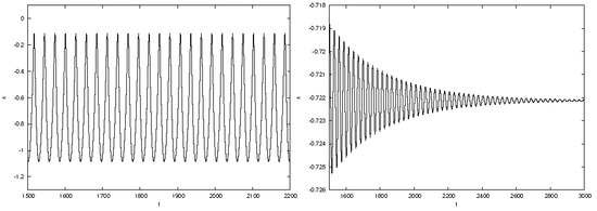
Figure 1. Time series of system (8), when (left) $\epsilon =0.12<{\epsilon }_c$ and (right) $\epsilon =0.13>{\epsilon }_c$.

3.1. ID-IO Polynomial

The package DifferentialAlgebra of Maple is used, in order to obtain the IO polynomial of the HR model. u is supposed to be an input of the system. To eliminate the variables $x_1$, $x_2$ and $x_3$ as well as to acquire relations between y, u and $\theta$, the elimination order $\left[\theta \right]\prec [y,u]\prec [x_1,x_2,x_3]$ is chosen. The Rosenfeld–Groebner algorithm provides a polynomial with a derivative of order 3, with 24 expressions. To obtain a simpler polynomial, let ${\displaystyle w_1\left(t\right)=e^{-t},v_1\left(t\right)=e^{-t}{\int }_0^t{x}_1^2(s,\theta )e^{s}ds}$. In integrating the second Equation of (8), one gets ${\displaystyle x_2(t,\theta )=(x_2(0,\theta )-1)w_1\left(t\right)+1-d{v}_1\left(t\right)}$. The following system is, now, considered:

$$\left\{\begin{array}{ccc}{\dot{x}}_1(t,\theta )& =& x_2(t,\theta )+a{x}_1^2(t,\theta )-x_1^3(t,\theta )-x_3(t,\theta )+u\left(t\right),\hfill \\ x_2(t,\theta )& =& (x_2(0,\theta )-1)w_1\left(t\right)+1-d{v}_1\left(t\right),\hfill \\ {\dot{x}}_3(t,\theta )& =& \epsilon (b(x_1(t,\theta )-c_{x_1})-x_3(t,\theta )),\hfill \\ {\dot{w}}_1\left(t\right)& =& -w_1\left(t\right),\hfill \\ {\dot{v}}_1\left(t\right)& =& -v_1\left(t\right)+x_1^2\left(t\right).\hfill \end{array}\right.$$

(9)

System (8) completed with the initial conditions $(x_1(0,\theta ),x_2(0,\theta ),x_3(0,\theta ))$ is equivalent to System (9) completed with $(x_1(0,\theta ),x_2(0,\theta ),x_3(0,\theta ),1,0)$. Considering now the elimination order $\left[\theta \right]<[y,w_1,v_1,u]\prec [x_1,x_2,x_3]$, we obtain (the time variable t is omitted): $P:=\ddot{y}+3y^2\dot{y}+(-\epsilon y_0+\epsilon +y_0-1)w_1+(d\epsilon -d)v_1+\epsilon (y^3+\dot{y})+(-a\epsilon +d)y^2-2ay\dot{y}+b\epsilon y-\epsilon (b{c}_y+1+u).$

Since the estimation of derivatives from noisy measurements is an ill-posed problem, some technicals were proposed to decrease the derivative orders of these polynomials. The most natural one is the integration of this IO polynomial, and the use of integration by parts.

The following relation, which does not contain any derivative, is, also, obtained:

$$\begin{array}{cc}{\displaystyle I_2\left(P\right)=}\hfill & {\displaystyle y\left(t\right)-2y(t-\tau )+y(t-2\tau )+{\int }_{t-\tau }^t(y{\left({\tau }_1\right)}^3-y{({\tau }_1-\tau )}^3)d{\tau }_1}\hfill \\ \hfill & {\displaystyle +(-\epsilon y_0+\epsilon +y_0-1){\int }_{t-\tau }^t{\int }_{{\tau }_1-\tau }^{{\tau }_1}{w}_1\left({\tau }_2\right)d{\tau }_{2}d{\tau }_1+(d\epsilon -d){\int }_{t-\tau }^t{\int }_{{\tau }_1-\tau }^{{\tau }_1}{v}_1\left({\tau }_2\right)d{\tau }_{2}d{\tau }_1}\hfill \\ \hfill & {\displaystyle -\epsilon \left(-{\int }_{t-\tau }^t{\int }_{{\tau }_1-\tau }^{{\tau }_1}y{\left({\tau }_2\right)}^{3}d{\tau }_{2}d{\tau }_1\right.\left.+{\int }_{t-\tau }^t(y\left({\tau }_1\right)-y({\tau }_1-\tau ))d{\tau }_1\right)}\hfill \\ \hfill & {\displaystyle +(-a\epsilon +d){\int }_{t-\tau }^t{\int }_{{\tau }_1-\tau }^{{\tau }_1}y{\left({\tau }_2\right)}^{2}d{\tau }_{2}d{\tau }_1-a{\int }_{t-\tau }^t(y{\left({\tau }_1\right)}^2-y{({\tau }_1-\tau )}^2)d{\tau }_1}\hfill \\ \hfill & {\displaystyle +b\epsilon {\int }_{t-\tau }^t{\int }_{{\tau }_1-\tau }^{{\tau }_1}y\left({\tau }_2\right)d{\tau }_{2}d{\tau }_1-(I\epsilon +b{c}_y\epsilon +\epsilon ){\tau }^2.}\hfill \end{array}$$

Evaluating this ID-IO polynomial at each $t_k$, $k=1,\dots ,N$ gives the following linear system.

$$0\in \left[\tilde{A}\right]\left[\tilde{x}\right]-\left[\tilde{b}\right]$$

(10)

where, if $\left[{\tilde{A}}_k\right]$ and $\left[{\tilde{b}}_k\right]$ represent the $k$th line (k from 1 to 7) of $\left[\tilde{A}\right]$ and $\left[\tilde{b}\right]$, respectively, then

$$\begin{array}{cc}{\left[b\right]}_j=\hfill & [y_j-2y_{j-\tau }+y_{j-2\tau }+I_1^j(y{(.)}^3-y{(.-\tau )}^3)],\hfill \\ {\displaystyle {\left[A\right]}_j=}\hfill & \left({\displaystyle \left[I_2^j\left(w_1\right)\right],\left[I_2^j\left(v_1\right)\right],[-I_2^j\left(y^3\right)-I_1^j(y(.)-y(.-\tau ))],\left[I_2^j\left(y^2\right)\right]}\right.,\hfill \\ \hfill & {\displaystyle \left.\left[I_1^j(y{(.)}^2-y{(.-\tau )}^2)\right],\left[I_2^j\left(y\right)\right],\left[{\tau }^2\right]\right).}\hfill \end{array}$$

In [5], the estimated parameters are obtained in solving the linear system $\tilde{A}\tilde{x}=\tilde{b}$ with the QR factorization, whereas, we propose in this paper to estimate the enclosure of the parameters in solving (10) with the SIVIA algorithm. The important differences, with respect to the previous paper, are summarized in the two structure diagrams Figure 2. In the left diagram, the stochastic procedure is presented. M is the number of iterations, to calculate the probability that the system reproduces the expected behavior of the model, given a numerical procedure and a noise. The right diagram summarizes the method presented in this paper, to estimate an enclosure of the parameters.

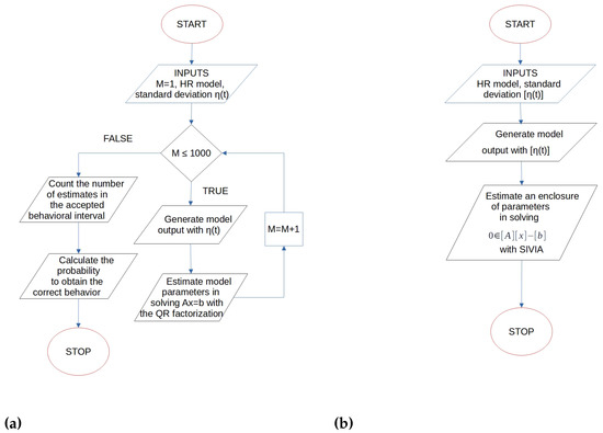
Figure 2. These two diagrams summarize the differences between the procedure presented in [5] and the one presented in this paper. (a) Diagram summarizing the stochastic procedure, presented in [5]. (b) Diagram summarizing the interval procedure, presented in this paper.

Let a parameter vector be given, for which the model solution is near an equilibrium point, such that one of the parameters is a bifurcation parameter. In our case, $\epsilon$ is the bifurcation parameter (see Section 3). The two works aim, also, to detect if the parameter value obtained by an optimization procedure leads to the expected behavior of the model output or not. The first method is based on the use of probabilistic tools. In contrast to this, the proposed method, based on interval arithmetic, is used to analyze the accuracy of the parameter identification algorithm. This new approach provides interval bounds, for all parameters to be identified, and in which the true parameters are located with 100% certainty, since the measurement noise is assumed to be bound. Consequently, this method allows for detecting, with certainty, the structural changes of the dynamics, by checking whether the parameter values corresponding to the bifurcation point are included or not in the estimated parameter ranges.

3.2. Parameter Estimation

In this section, enclosures of different integrals in the set-membership framework are obtained, by the interval extension of the trapezoidal classic method.

For the simulations, the following values are taken: $a^{*}=3$, $b^{*}=4$, $d^{*}=5$, $u\left(t\right)=3.25$A, ${\epsilon }^{*}=0.20$, $(x_1(0,\theta ),x_2(0,\theta ),z(0,\theta ))=(0.2;0.7;4)$. The time interval is $[0,1000]$, with a step size $h=0.01$s.

The integrals are evaluated, by using 29 points. In the output equation, $\left[\eta \right(t\left)\right]$ is given by three successive intervals: $[0.00008,0.00012]$, $[0.0004,0.0006]$ and $[0.0005,0.0015]$, then System (10) is solved by using SIVIA’s algorithm (see Section 2.3). For each instance of this value, the estimated intervals of $\tilde{a}$, $\tilde{b}$, $\tilde{d}$, $\tilde{\epsilon }$ and the widths of the estimated intervals are given in Table 1 and Table 2.

Table 1. Parameter values obtained with the method presented in Section 2.

$\left[\mathit{\eta }\right(\mathit{t}\left)\right]$	$\tilde{\mathit{\epsilon }}$	$\tilde{\mathit{a}}$	$\tilde{\mathit{b}}$	$\tilde{\mathit{d}}$
$[0.00008,0.00012]$	$[0.1949,0.2029]$	$[2.9300,3.0600]$	$[3.9790,4.1156]$	$[4.9399,5.0681]$
$[0.0004,0.0006]$	$[0.1934,0.2035]$	$[2.9398,3.0633]$	$[3.9089,4.0225]$	$[4.9407,5.0654$
$[0.0005,0.0015]$	$[0.1905,0.2024]$	$[2.9563,3.0643]$	$[3.8557,4.1684]$	$[4.9409,5.0670]$
$[-0.0001,0.0001]$	$[0.1369,0.2026]$	$[2.9909,3.2119]$	$[3.3170,5.1301]$	$[4.9709,5.1399]$
$[-0.0001,0.0001]$	$[0.18,0.2026]$	$[2.9909,3.2119]$	$[3.6,.4]$	$[4.9709,5.1399]$

Table 2. Widths of estimated parameter intervals, obtained with the method presented in Section 2.

$\left[\mathit{\eta }\right(\mathit{t}\left)\right]$	$\tilde{\mathit{\epsilon }}$	$\tilde{\mathit{a}}$	$\tilde{\mathit{b}}$	$\tilde{\mathit{d}}$
$[0.00008,0.00012]$	0.0089	0.1300	0.1366	0.1282
$[0.0004,0.0006]$	0.0101	0.1235	0.1136	0.1247
$[0.0005,0.0015]$	0.0119	0.1080	0.3127	0.1261
$[-0.0001,0.0001]$	0.0657	0.2210	1.8131	0.1690

The impact of the width of the interval chosen for the measurement noise is analyzed through the width of the estimated.

The intervals for initial values are given by $\epsilon \in [0.18,0.22]$, $a\in [2.7,3.3]$, $b\in [3.6,4.4]$ and $d\in [4.5,5.5]$.

All the intervals in Table 1 and Table 2 contain the true values. Table 1 and Table 2 highlight the impact of the width of the measurement noise interval on the width of the estimated; the larger the size of this interval is, the larger the size of the estimates.

4. Conclusions

In this paper, a new approach to estimate unknown parameters of the HR model is considered in the set-membership framework, to detect, with certainty, a behavior change in the dynamic of the system. Indeed, unlike probabilistic methods, which only give the probability that the estimated parameter leads to the expected behavior, the method we propose certifies whether the parameter values corresponding to the bifurcation parameter are included or not in the estimated parameter ranges. It takes the benefit of the differential algebra-based method, integration and the SIVIA algorithm. Numerical simulations highlight the interest of the proposed approach, in terms of estimated interval widths, compared to the previous approaches that are based on IO polynomials. A sensitivity analysis of estimates to the noisy data will be the subject of future works, as this could, indeed, improve the estimation of the parameters, based on the works of [25].

References

- Boulier, F.; Lazard, D.; Ollivier, F.; Petitot, M. Computing Representation for Radicals of Finitely Generated Differential Ideals; Technical Report; Université Lille I: Villeneuve d’Ascq, France, 1997. [Google Scholar]
- Loeb, J.; Cahen, G. More about process identification. Automatica 1965, 10, 359–361–447. [Google Scholar] [CrossRef]
- Sira-Ramirez, H.; Rodriguez, C.G.; Romero, J.C.; Juárez, A.L. Algebraic Identification and Estimation Methods; Feedback Control Systems; Wiley: Hoboken, NJ, USA, 2014. [Google Scholar]
- Verdière, N.; Jauberthie, C.; Travé-Massuyès, L. Improvements in bounded error parameter estimation using distribution theory. In Proceedings of the European Control Conference 2018, Limassol, Cyprus, 12–15 June 2018; pp. 2460–2465. [Google Scholar]
- Verdière, N.; Jauberthie, C. Parameter Estimation Procedure Based on Input-Output Integro-Differential Polynomials. Application to the Hindmarsh-Rose Model. In Proceedings of the European Control Conference 2020, Saint Petersbourg, Russia, 25 November 2020; pp. 220–225. [Google Scholar]
- Jaulin, L.; Kieffer, M.; Didrit, O.; Walter, E. Applied Interval Analysis: With Examples in Parameter and State Estimation, Robust Control and Robotics, 1st ed.; An Emerging Paradigm; Springer: Berlin/Heidelberg, Germany, 2001. [Google Scholar]
- Boulier, F.; Korporal, A.; Lemaire, F.; Perruquetti, W.; Poteaux, A.; Ushirobira, R. An Algorithm for Converting Nonlinear Differential Equations to Integral Equations with an Application to Parameter Estimation from Noisy Data. In Proceedings of the Computer Algebra in Scientific Computing 2014, Warsaw, Poland, 8–12 September 2014; pp. 28–43. [Google Scholar]
- Hindmarsh, J.; Rose, R. A model of the nerve impulse using two first-order differential equations. Nature 1982, 296, 162–164. [Google Scholar] [CrossRef] [PubMed]
- Hindmarsh, J.; Rose, R. A model of neuronal bursting using three coupled first order differential equations. Proc. R. Soc. Lond. Biol. Sci. 1984, 221, 87–102. [Google Scholar]
- Hodgkin, A.L.; Huxley, A.F. A quantitative description of membrane current and its application to conduction and excitation in nerve. J. Physiol. 1952, 117, 500–544. [Google Scholar] [CrossRef] [PubMed]
- Izhikevich, E.M. Dynamical Systems in Neuroscience; MIT Press: Cambridge, MA, USA, 2007. [Google Scholar]
- Tokuda, I.; Parlitz, U.; Illing, L.; Kennel, M.; Abarbanel, H. Parameter estimation for neuron models. In Proceedings of the AIP Conference, San Diego, CA, USA, 26–29 August 2003. [Google Scholar]
- Corson, N.; Lanza, V.; Verdière, N. Hopf bifurcations in a chain of coupled Hindmarsh-Rose system. Acta Biotheor. 2016, 65. [Google Scholar]
- Schumann-Bishoff, J.; Parlitz, U. State and parameter estimation using unconstrained optimization. Phys. R. E 2011, 84., 375–402. [Google Scholar] [CrossRef] [PubMed]
- Steur, E. Parameter Estimation in Hindmarsh-Rose Neurons. Ph.D. Thesis, Technische Universiteit Eindhoren, Eindhoven, The Netherlands, 2006. [Google Scholar]
- Denis-Vidal, L.; Joly-Blanchard, G.; Noiret, C.; Petitot, M. An algorithm to test identifiability of non-linear systems. In Proceedings of the 5th IFAC NOLCOS, Saint Petersburg, Russia, 4–6 July 2001; pp. 174–178. [Google Scholar]
- Jauberthie, C.; Verdière, N.; Travé-Massuyès, L. Fault detection and identification relying on set-membership identifiability. Annu. Rev. Control. 2013, 37, 129–136. [Google Scholar] [CrossRef] [Green Version]
- Fliess, M.; Mboup, M.; Mounier, H.; Sira-Ramirez, H. Questioning Some Paradigms of Signal Processing via Concret Examples. Available online: https://hal.inria.fr/inria-00001059/file/signalg.pdf (accessed on 7 April 2022).
- Jaulin, L.; Walter, E. Set inversion via interval analysis for nonlinear bounded-error estimation. Automatica 1993, 29, 1053–1064. [Google Scholar] [CrossRef]
- Rauh, A.; Dötschel, T.; Auer, E.; Aschemann, H. Interval Methods for Control-Oriented Modeling of the Thermal Behavior of High-Temperature Fuel Cell Stacks. IFAC Proc. Vol. 2012, 45, 446–451. [Google Scholar] [CrossRef]
- Rauh, A.; Kersten, J.; Aschemann, H. An Interval Approach for Parameter Identification and Observer Design of Spatially Distributed Heating Systems. IFAC-PapersOnLine 2018, 51, 337–342. [Google Scholar] [CrossRef]
- AbdelAty, A.M.; Fouda, M.E.; Eltawil, A. Parameter Estimation of Two Spiking Neuron Models With Meta-Heuristic Optimization Algorithms. Front. Neuroinform. 2022, 16. [Google Scholar] [CrossRef] [PubMed]
- Lynch, E.P.; Houghton, C.J. Parameter estimation of neuron models using in-vitro and in-vivo electrophysiological data. Front. Neuroinform. 2015, 9, 10. [Google Scholar] [CrossRef] [PubMed] [Green Version]
- Jauberthie, C.; Travé-Massuyès, L.; Verdière, N. Set-membership identifiability of nonlinear models and related parameter estimation properties. Int. J. Appl. Math. Comput. Sci. 2016, 26, 803–813. [Google Scholar] [CrossRef] [Green Version]
- Rihan, F.A. Sensitivity analysis for dynamic systems with time-lags. J. Comput. Appl. Math. 2003, 151, 445–462. [Google Scholar] [CrossRef] [Green Version]
Publisher’s Note: MDPI stays neutral with regard to jurisdictional claims in published maps and institutional affiliations. |
© 2022 by the authors. Licensee MDPI, Basel, Switzerland. This article is an open access article distributed under the terms and conditions of the Creative Commons Attribution (CC BY) license (https://creativecommons.org/licenses/by/4.0/).