A Data-Driven Fault Tree for a Time Causality Analysis in an Aging System

Abstract

This paper develops a data-driven fault tree methodology that addresses the problem of the fault prognosis of an aging system based on an interpretable time causality analysis model. The model merges the concepts of knowledge discovery in the dataset and fault tree to interpret the effect of aging on the fault causality structure over time. At periodic intervals, the model captures the cause–effect relations in the form of interpretable logic trees, then represents them in one fault tree model that reflects the changes in the fault causality structure over time due to the system aging. The proposed model provides a prognosis of the probability for fault occurrence using a set of extracted causality rules that combine the discovered root causes over time in a bottom-up manner. The well-known NASA turbofan engine dataset is used as an illustrative example of the proposed methodology.

1. Introduction

The aging of a system is characterized by the progressive deterioration of its initial performance over time, including—among other factors—the occurrence of faults that adversely affect the system’s reliability [1]. Causality analysis methods aim to diagnose the fault event through identifying, isolating and quantifying the effect of the root causes on the system performance so that the appropriate maintenance actions can be performed to restore the system to good condition [2]. The future fault behaviour and its drawback on the system’s performance are essential in order to optimize the maintenance decision-making [3]. Gao et al. [4] proposed a comprehensive survey of real-time fault diagnosis methods that are mainly categorized into model-, signal-, and knowledge-based techniques. The fault prognosis task provides a model that depicts the progression of a specific failure mode from its inception until the time of failure [5]. The time causality analysis builds a prognostic model that captures the fault causality behaviour over time [6].

A prognostic model may use a mathematical expression that quantifies the fault causality evolution or a graphical representation that depicts the changes in the causality structure over time [7]. Both the event-based and the data-driven methods are commonly deployed to provide relevant fault prognostic models. The event-based method requires the involvement of experts from different fields with detailed prior knowledge about the fault time causality. However, this knowledge could be biased and reflects only the expert opinions about the fault development [8]. On the other hand, the data-driven method can directly extract the fault evolution knowledge from the data, which is unbiased knowledge and reflects the fault causality. However, it lacks the interpretability and the expert knowledge representation to identify fault hierarchical causality over time [9].

Waghen and Ouali [10] have developed a data-driven fault tree method for causality analysis which addresses the lack of interpretability of the data-driven model and overcomes the model-based limitation regarding the expert prior knowledge. The method visualizes the fault causality architecture of a simple system using one-level fault tree that consists of three layers. The condition layer identifies the fault root causes and their coverage ranges within the dataset. The pattern layer arranges the root causes in the form of interpretable conjunctions. The solution layer combines some selected patterns that depict the fault event. Although the proposed tree is interpretable for the expert, the model hides the fault hierarchical cause-and-effect relations in a complex system. Moreover, it reflects the fault causality in a static way without considering the influence of a system’s aging on the change in the fault causality structure over time.

From a practical point of view, human experts look for models that are able to explain and represent the fault causality structure in addition to having prediction capability. Ensuring that the fault and its impact and consequences are well represented to human experts guarantees optimal preventive maintenance actions. Another challenge in a complex system with regard to data-driven fault prognosis models is graphically modeling the deterioration and performance degradation. Consequently, the fault causality structure can be changed over a system’s life. Therefore, these complex systems need models that are able to capture these changes in an interpretable manner. This is a crucial feature that helps anticipate the impacts of a fault and provides more precise knowledge about the processes that will be affected in the future by a currently occurring fault.

In this paper, an interpretable time causality analysis (ITCA) methodology is developed to address the problem of fault prognosis in an aging system using a data-driven fault tree model. We aim to build a time-dependent multilevel causality model based on the selection of feasible solutions that characterize the fault occurrence at a certain period from a set of representative time series historical datasets to address the causality analysis over time in a meaningful way. The ITCA model is a combination of different common one-level fault trees that depict the changes of the fault causality structure at periodic intervals. At each defined period, the ITCA methodology identifies, isolates, and represents the possible causes of the fault event in the form of the interpretable one-level fault tree. These constructed trees over defined periods are merged into a common one-level fault tree that graphically summarizes the changes in the fault causality structure over time. This procedure is iteratively repeated for each unexplained cause from the previous level until the final multilevel ITCA model is constructed. The proposed construction procedure ensures that redundant knowledge is eliminated within the ITCA model, while maximizing its interpretability over the time. Finally, a set of causality rules are deduced from the ITCA fault tree that characterize the dynamic change effect of the causality structure in the causes of a fault occurrence.

The rest of the paper is organized into four sections. Section 2 reviews the available methods for achieving the fault prognosis based on time causality analysis and discusses the main challenges. Section 3 develops the ITCA methodology. It explains the data preparation, the construction of the fault tree models over time, and the deduction of the time causality rules for fault prognosis. Section 4 illustrates the ITCA methodology using the NASA turbofan engine degradation dataset. The performance of the ITCA model to predict the fault is demonstrated by the fault trend over time. Section 5 concludes the paper and discusses the contribution of the ITCA methodology in achieving the fault prognosis task.

2. Time Causality Analysis Methods

Time causality analysis is a causal interference over time where the temporary dependency between events over the stochastic process is captured and represented using analytical methods. The time causality analysis can achieve the fault prognosis task by providing the expert with the essential knowledge regarding the fault evolution and the change in its causality structure over time [11]. Schwabacher distinguishes the model-based and data-driven methods to address the fault prognosis issue. In what follows, a brief literature review of each prognostic method is discussed, and their strengths and limitations are highlighted to clarify the research gap [7].

The model-based method for time causality analysis relies heavily on human expertise to describe the system’s behaviour over time in degraded conditions [12]. Lu, Jiang [13] address the drawback of the system downtime due to fault evolution in complex industrial process by expert knowledge enrichment. First, the time-delayed mutual information (TDMI) is employed to model the fault causality in the form of a time-delayed signed digraph (TD-SDG) mode. Then, a general fault prognosis strategy is used to optimize the system’s downtime based on TD-SDG and the principal component analysis (PCA) technique. Darwish, Almouahed [14] propose an enriched fault tree for Active Assisted Living Systems (AALS). The fault tree basic events are ranked according to the degree of their importance based on the expert prior knowledge and the imprecise failure probabilities of those basic events. Ragab, El Koujok [15] combine the domain knowledge with the extracted knowledge from the database to build an enriched fault tree. First, the expert constructs the fault tree skeleton, which represents the main causality structure for the fault event. Then, some extracted patterns from the database that may depict unknown combinations of root causes are deployed to enrich the initial fault tree. Yunkai, Bin [16] integrate the bond graph modelling technique with the Bayesian network to predict the faults in a high-speed train traction system. The bond graph represents the system structure that is mainly constructed based on expert prior knowledge, while the Bayesian network enriches the expert prior knowledge represented by the bond graph through discovering the hidden causal relations.

Indeed, the model-based time causality approach can provide interpretable and relatively accurate models that can be built from the first principle of the system’s faults. It is mainly applicable on simple systems with well-known causes where human knowledge about the faults, their occurrence and development is clear. Its limited implementation in complex systems has been overcome by enriching those models based on data-driven techniques, in which the unseen events are discovered and added to the model’s prior knowledge. However, forming the model skeleton prior to knowledge by the expert in complex systems to identify the principal causality structure of the faulty situation and combining and positioning the extracted hidden fault knowledge from the data in the constructed model is a challenging task.

Unlike the model-based methods, the data-driven time causality method explores the data using machine learning (ML) techniques and does not impose a model to predict the behaviour of a complex system [17]. The ML data-driven methods build unbaised models and are able to deal with noisy and correlated variables [18]. Zhang, Wang [19] proposed a methodology to predict the remaining useful time (RUL) using the Wavelet Packet Decomposition of the vibration signal and Fast Fourier Transform. The pre-processed signals are treated as input features to learn the Artificial Neural Network (ANN) that predicts the RUL. Wu, Ding [20] implemented the long short-term memory (LSTM) neural network rather than relying on feature engineering and an ANN for fault prognosis in aircraft turbofan engines. The main advantage of LSTM over an ANN is its ability to learn long-term dependencies between input features and over the equipment lifetime to give accurate RUL prediction. Razavi, Najafabadi [21] developed an adaptive neuro-fuzzy inference system (ANFIS) algorithm that combines the ANN and a fuzzy rule-based model to predict the RUL of aircraft engines. The ANFIS algorithm has been applied to maintenance scheduling problems.

Although the data-driven models offer an accurate prediction of the RUL, they suffer from a lack of interpretability [22]. This is because they are too shallow to understand the fault causality structure and its changes over time. Therefore, an expert may not be able to deeply understand the cause–effect relations within a complex system. With regard to this challenge, several methods have been proposed to simplify and unlock the model interpretability. Li, Wang [23] employed the Deep Belief Network (DBN) to model the geometric error structure of the backlash error. The DBN was built using restricted Boltzmann machines and energy-based models to predict the fault geometric. Su, Jing [24] have proposed a dynamic extraction knowledge method that illustrates the relationship between the environmental stresses and the system failure modes using a fuzzy causality diagram and a Bayesian rough set of multiple decision classes to weigh the extracted knowledge. Kimotho, Sondermann-Woelke [25] addressed the challenge of maintenance action recommendation for industrial systems based on remote monitoring and diagnosis. They proposed an interpretable event-based decision tree that graphically identifies some problems associated with particular events and conducts evidence-based decisions. Medjaher, Moya [26] used Dynamic Bayesian Networks (DBNs) to quantify the failure prognostic in complex systems. The fault time series data are divided into several periods and a Bayesian network is constructed for each period. The obtained networks are connected through the chronology of periods to depict the changes in the fault causality structure over time and quantify the fault behaviour.

On the other hand, the achieved data-driven methods attempt to unlock the time-dependent relations between the system variables in an interpretable manner in addition to capturing the change in the fault causality through the periods. However, building an interpretable data-driven model that can directly grasp the influence of the system aging on the fault causality structure and summarize the fault behaviour in one model, is a challenge that still needs to be overcome. The main motivation of this study is to build an interpretable time causality analysis model that characterizes, first, the hierarchical causality structure between the fault event, intermediate causes, and root-causes; and second, the influence of the system aging on that structure over time. Thus, the proposed ITCA methodology will achieve the fault prognosis task in an efficient way through anticipating the fault event based on the causal relations discovered over time. It will be developed in the following section.

3. The ITCA Methodology

Figure 1 depicts the four-phase ITCA methodology. The main input dataset is an unlabelled timestamp of observations that can represent sequential data. We assume that the system undergoes a certain degradation trend, depicted by the sequential data, from a normal state to a failure state, represented by green and red colors, respectively. Phase 1 prepares several labelled subsets from the input data. Each subset is formed by a sub-sequence of degraded observations, beginning from normal observations (green colors) to failure ones (red colors), gradually. Phase 2 iteratively builds the appropriate logic tree corresponding to each subset of data, and then aggregates them into one common fault tree. Phase 3 constructs the ITCA model by going deeply through each variable in the above common fault tree and seeks its root-causes. Phase 4 deduces the time causality rules that determine the effects that the system aging has on the evolution of the fault occurrence over time. In what follows, each phase of the proposed methodology is explained in detail.

3.1. Phase 1: Data Preparation

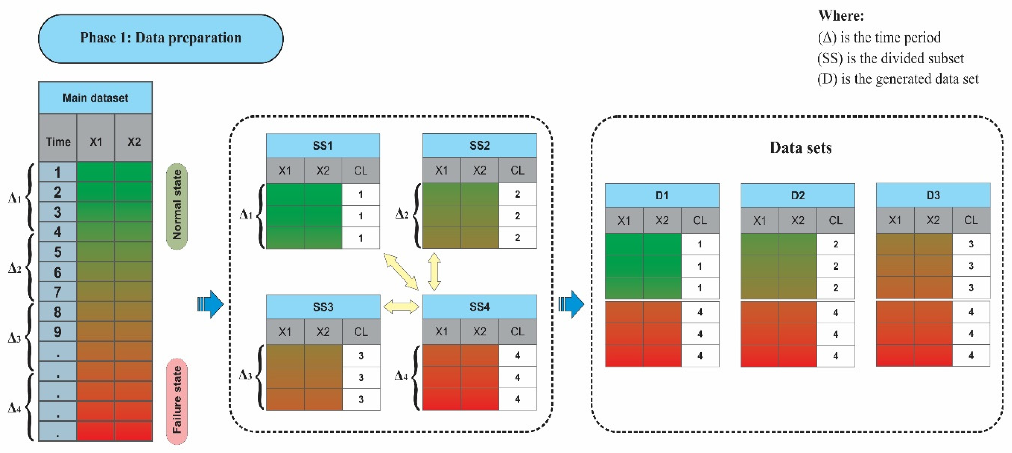
Phase 1 splits the main input data into several subsets according to the expert’s prior knowledge about the process degradation trend. Each subset contains the sequential observations that represent the system state at a certain period and the observations that characterise the failure state or the worst deterioration condition of the system. The expert should identify the observations that represent the failure before splitting the rest of the data into equal or non-equal sizes of subsets, according to his judgment about the amount of system degradation. Equal and non-equal sizes of subsets are suitable for linear and nonlinear degradation processes, respectively. Hence, the original main data are divided into n subsets, where the last one contains the failure observations and the others contain degraded observations. Those n subsets will be concatenated to form (n − 1) datasets. Each dataset will contain two classes of observations corresponding to failure and degraded data.

Figure 2 depicts the data preparation procedures, in which X₁ and X₂ are two variables. Beginning from the main timestamped dataset, the observations in the last period Δ_n belong to the failure state. Then, (n − 1) subsets are extracted. Each subset SS_i contains the observations of the period Δ_i, I = 1, …, J, where (j) is the index of the last observation for a given period. At the end, (n − 1)-labelled datasets are concatenated. Each dataset D_i contains the observations of the period Δ_i, labelled as class i and the observations of the last period Δ_n, labelled as class n.

3.2. Phase 2: Build a One Level Fault Tree

Phase 2 iteratively extracts all of the logic trees that differentiate the fault event (class n) from each class i, i = 1, …, (n − 1) of the degraded observations individually. Each logic tree highlights the relevant variables that discriminate the observations of the failure state from the degraded ones, from one period to another. Then, the obtained logic trees are merged into one common fault tree, which identifies and isolates the variables that discriminate the failure state from the degraded ones over time. To do so, Waghen and Ouali [10] developed a four-stage methodology, named Interpretable Logic Tree Analysis (ILTA), to build a one-level fault tree from a two-class dataset (i.e., normal and failure classes). The methodology discovers the knowledge from the dataset (Stage 1); forms feasible solutions (Stage 2); constructs the fault tree (Stage 3); and finally quantifies the fault tree using Bayes’ theorem (Stage 4). Although such a methodology can be applied separately with each dataset D_i, i = 1, …, (n − 1), the merged fault tree may be difficult to interpret due to the dependence of the datasets over time. To overcome this limitation, Stage 2 of the ILTA methodology needs to be improved. Nevertheless, for the convenience of the reader, we briefly recall the four stages of the ILTA methodology and highlight the improvements to Stage 2 in the following.

• Stage 1: Discover knowledge. Discovering knowledge from a two-class dataset can be achieved through different pattern generation and extraction techniques, such as the logic analysis of data (LAD) [27] and prediction rule ensembles (PRE) [28]. The pattern is a conjunction of certain conditions that discriminate one class of observations from another class. Each condition includes a variable, an inequality sign, and a cut point value. Furthermore, the percentage of observations covered by a given pattern may characterize the knowledge expanse caught by that pattern. However, when the observations of the same class are covered by more than one pattern, an overlap between those patterns may occur, with a certain percentage leading to redundant knowledge.
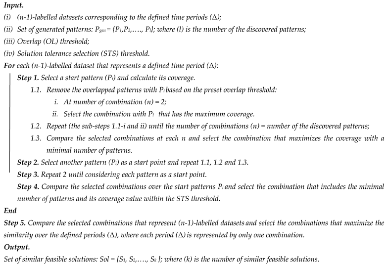
• Stage 2: Obtain similar feasible solutions. A solution is defined as a combination of certain patterns that cover the observations of the same class. Each solution can be characterized by its coverage (Cov) and overlap (OL) percentages. The feasible solution is a solution that respects certain criteria. In the ILTA methodology, only the feasible solution that maximizes the class Cov and minimizes the class OL is selected, which leads to maximizing the interpretability and minimizing the redundancy of the discovered knowledge. However, in the ITCA methodology, we need to search for all of the feasible solutions that respect not only the Cov and OL threshold percentages, but also with minimal number of patterns to capture the common knowledge at the same level over time. In other words, the minimal number of patterns having the maximum Cov and the minimum OL allows us to characterize the fault using global knowledge at the first levels of the tree. When this causality is represented in the tree and the related knowledge is removed from the dataset, the subsequent feasible solutions will reveal other knowledge that depicts sub-causalities not yet discovered and represented in the tree. As Stage 2 aims to select similar feasible solutions that characterize knowledge discovery over time, we seek the most frequent patterns over the predefined periods of time. In addition, the frequent pattern involves the same variable and inequality sign in the shared conditions, independent of the cut-point values. Therefore, the initial version of the burn-and-build algorithm proposed in [10] is improved to form a set of feasible solutions instead of only one for each period, using another decision criterion called the solution tolerance selection (STS) threshold. Hence, a time-based searching algorithm is developed in the ITCA methodology to obtain all the similar feasible solutions over time. It is depicted in the following Algorithm 1.

Algorithm 1. Time-based searching algorithm: Search for similar feasible solutions over time.

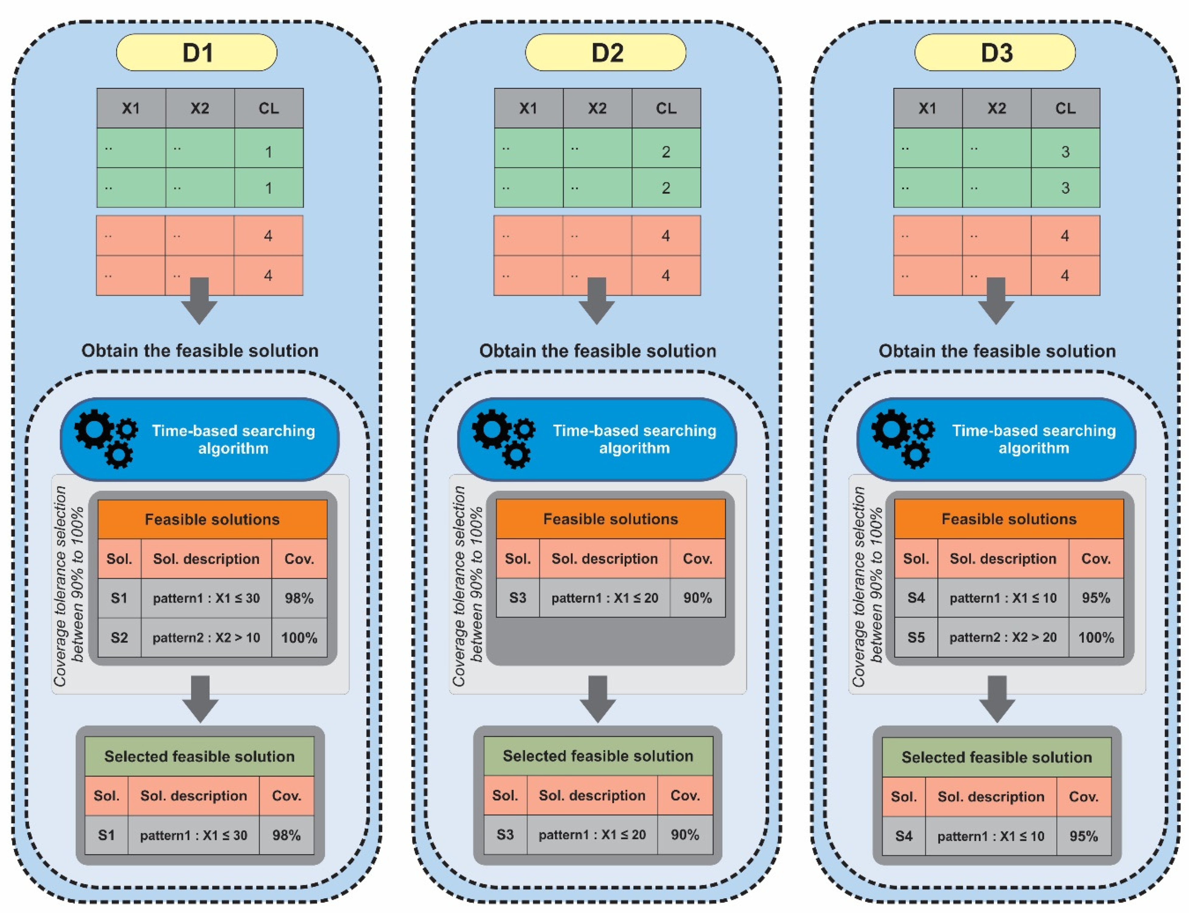
Figure 3 illustrates the proposed time-based searching algorithm using the above three concatenated datasets $D_1$, $D_2$ and $D_3$ of the toy example (Figure 1). Applying Step 1 to Step 4, the algorithm finds a set of five feasible solutions that respect the STS threshold of 90%. To clearly understand this, we assume that each solution consists of only one pattern. From $D_1$, $S_1:P_1:\left(X_1\le 30\right)$ and $S_2:P_2:(X_2>10)$ are obtained with 98% and 100% of Cov, respectively. From $D_2$, there is only one formed solution $S_3:P_3:(X_1\le 20$) with a Cov of 90%. From $D_3$, the obtained solutions $S_4:P_4:\left(X_1\le 10\right)$ and $S_5:P_5:(X_2>20)$ have 95% and 100% Cov, respectively. Note that the patterns $P_1$, $P_3$ and $P_4$ share the same condition on $X_1$ except the cut points. Consequently, at Step 5, the algorithm selects $S_1$, $S_3$ and $S_4$ as the only three similar solutions that characterize the evolution of the same condition through the three periods Δ₁, Δ₂, and Δ₃, respectively. However, the algorithm does not select $S_2$ and $S_5$ because there is a loss of information during the period Δ₂, even though they are similar, by sharing the same condition of $X_2$ during Δ₁ and Δ₃. Hence, the algorithm evaluates all of the similar feasible solutions and selects the ones that dominate the maximum number of periods.

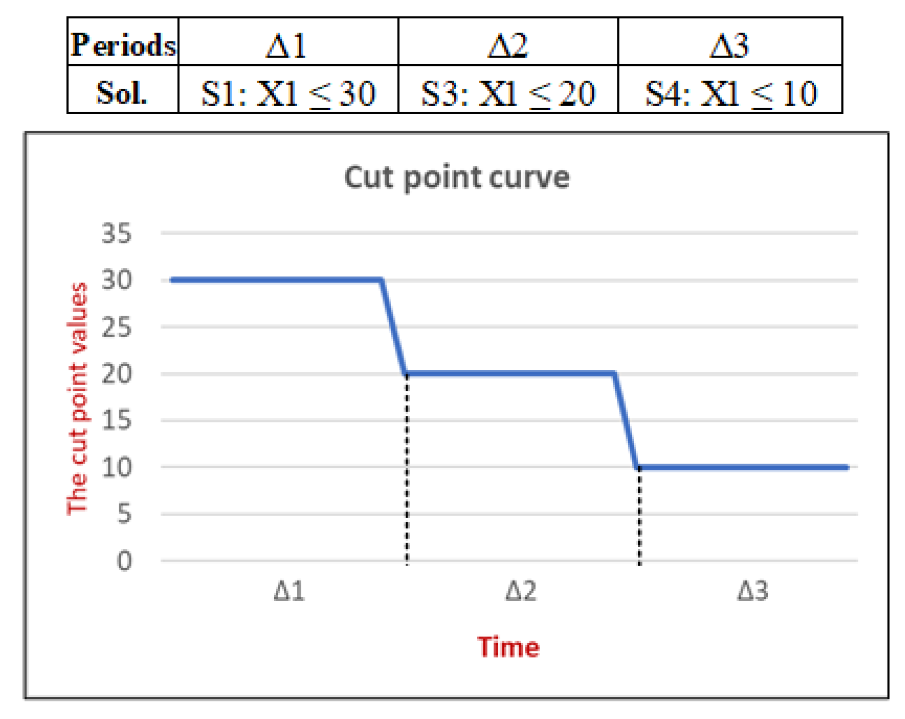
Figure 4 depicts the curve of the cut-point values that reflect the evolution of similar feasible solutions obtained over the three periods Δ₁, Δ₂, and Δ₃. Note that these periods are consecutive, and the cut-point curve may have a positive, negative, or constant trend over time depending on how the cut-point values change over time.

• Stage 3: Construct a common logic tree over time. The similar feasible solutions obtained are visualized in a one-level fault tree through the condition, pattern, and solution layers. At the condition layer, all the involved conditions are connected to their respective patterns using the AND gate. At the pattern layer, all the patterns of the similar feasible solutions are connected to that solution using the OR gate. Similarly, at the solution layer, all the selected similar feasible solutions are connected to the fault event using the OR gate.
• Stage 4: Assign the probabilities. The common logic tree is quantified using the probabilities of the solutions, patterns and conditions involved in similar feasible solutions obtained from the concatenated dataset individually. Let $N_k$ and $N_T$ be the number of observations covered by the condition $C_k$ and the total number of observations in one concatenated dataset, respectively. Equations (1) to (4) calculate the probabilities of the fault class $\mathcal{P}\left(CL\right)$ and the involved solutions $\mathcal{P}\left(S_q\right) q=1,2, \dots Q$, patterns $\mathcal{P}\left(P_j\right) j=1..J$, and conditions $\mathcal{P}\left(C_k\right) k=1..K$ as follows:

  $$\mathcal{P}\left(C_k\right)=\frac{N_k}{N_T}$$

  (1)

  $$\mathcal{P}\left(P_j\right)={\displaystyle \prod }_{k=1}^{n_j-1}\mathcal{P}\left(C_k\mid C_{k+1}\right)\cdot P\left(C_{k+1}\right)$$

  (2)

  $$\mathcal{P}\left(S_q\right)=\mathcal{P}\left[{\displaystyle \mathrm{\bigcup }}_{j=1}^J{P}_j\right]$$

  (3)

  $$\mathcal{P}\left(CL\right)=\mathcal{P}\left[{\displaystyle \mathrm{\bigcup }}_{q=1}^Q{S}_q\right]$$

  (4)

For a simple cause–effect relation between the fault event and its root causes, the common one-level logic tree can depict the fault causality structure at each period, as well as over time through the trend of cut-point curves of similar feasible solutions employed in the tree. For a complex causality structure, the one-level logic tree is not sufficient to completely represent a fault occurrence because the variables involved at the condition layer may represent the intermediate causes, and not necessarily the root causes of the fault event. Therefore, each one of those variables needs a second level of decomposition or more to explore the solution that will explain its causality structure at each period. Accordingly, Phase 3 constructs many levels of the tree to address the complex causality structure over time.

3.3. Phase 3: The ITCA Model Construction

Phase 3 builds, in a sequential up-bottom structure, several connected common logic trees to depict unexplained causes through multilevel structure. Each level includes three stages: verify the common logic trees’ construction, connect those trees to their corresponding causes, and generate new labelled sub-datasets that exclude the variables associated with causes already explained from the concatenated datasets. In Phase 3, each cause (i.e., condition) of the obtained common logic trees in Phase 2 is considered as a new event that needs to be explained in a lower level using a new common logic tree. This procedure is iteratively repeated to construct a multilevel tree that represent the fault causality structure over time. In such hierarchical structures, the common feasible solutions at the first level characterize the fault event using general fault indicators, while the common feasible solutions at the lower levels will use specific fault indicators to explain the last causes of the tree.

• Stage 1: Verify the common logic trees’ construction over the defined periods. This stage verifies the knowledge representability of the constructed logic tree for each defined period of time and decides whether the further decomposition of its involved condition is required or not. At each decomposition level, verification of the tree knowledge is characterized by the coverage of the common feasible solution, which assists in avoiding decomposing the weak information branches. Therefore, the model construction is verified to sustain the tree at a non-redundant knowledge level based on the pre-set coverage threshold. Meanwhile, the construction phase can be interpreted if there is no common tree that is able to provide sufficient knowledge representability, or if there are no more variables in the dataset for any further root cause explorations.
• Stage 2: Connect the common logic trees to their corresponding causes. The applied relaxation in selecting a common feasible solution over the defined periods is very useful in constructing a common logic tree that easily demonstrates the change in the causality at a given level of decomposition in the ITCA model. However, it could happen if the time-based searching algorithm fails to form only one common logic tree that dominates all the defined periods at a certain decomposition level. This case could happen if there is a lack of extracted knowledge or a tight range in the solution tolerance selection (STS). To solve this situation, different common logic trees may be found by the algorithm, but each period is dominated by only one common feasible solution. Therefore, if such a situation rises, a time–OR gate is proposed to connect the different common logic trees to represent the change in the event causality knowledge over all the defined periods at a given decomposition level. The time–OR gate acts as a time switch that shifts between the common logic trees according to their corresponding periods. Hence, an expert could observe the fault behaviour over time based on the proposed common similar solution trees at a certain decomposition level of the ITCA model.

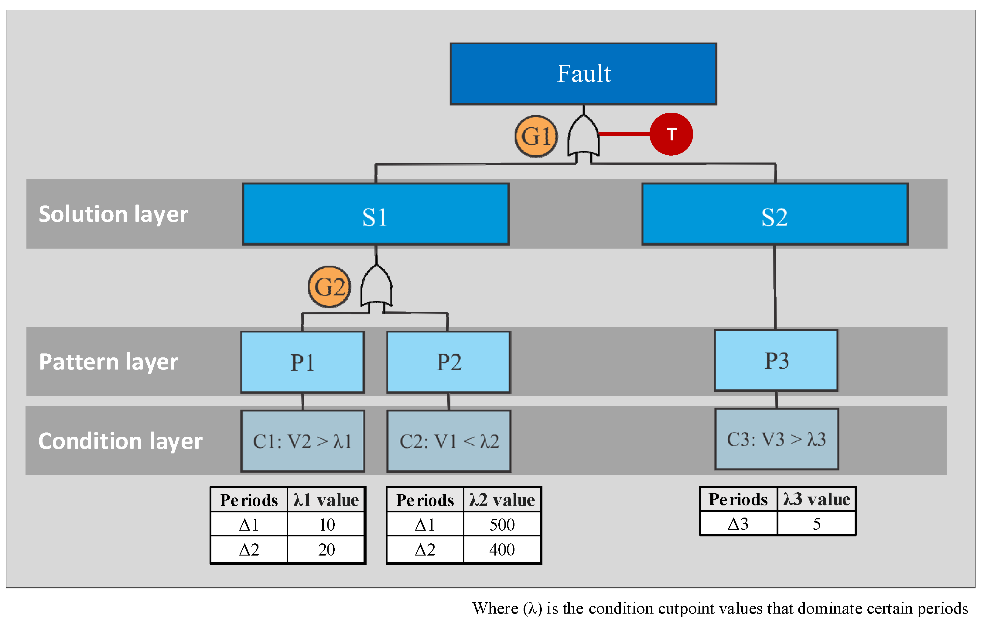
Figure 5 presents an example of the time–OR gate functionality in a one-level ITCA model. Two common feasible solutions, $S_1$ and $S_2,$ are found by the time-based searching algorithm. $S_1$ characterizes the fault event at only Δ₁ and Δ₂ using the OR gate (G2) between the patterns $P_1$ and $P_2$. While $S_2$ represents the fault even only at only Δ₃ with one pattern, $P_3$. This allows $P_3$ to be connected directly to $S_2$ without any need for an OR gate. The time–OR gate (G1) enables ITCA to fully demonstrate the fault event causality over the three defined periods (Δ₁, Δ₂ and Δ₃). It switches between $S_1$ and $S_2$ according to the selected corresponding period that is dominated by the solution. For instance, at the periods Δ₁ and Δ₂, the time–OR gate (G1) enables only $S_1$ to depict the fault event causality. On the other hand, during the period Δ₃, the fault causality is explained only by $S_2$.

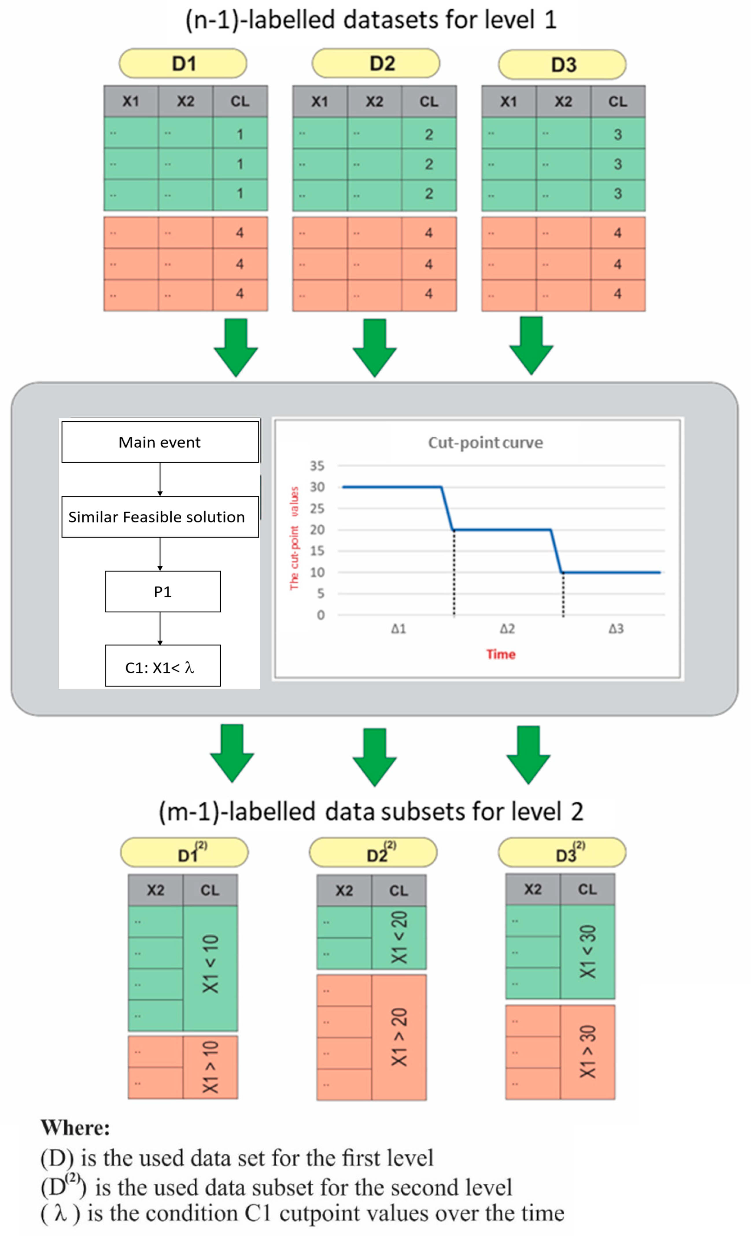
• Stage 3: Generate new (m − 1) sub-datasets. In a case in which the added common logic trees are verified at a certain decomposition level of the ITCA model, each one of the involved conditions in the tree is used to generate new labelled sub-datasets based on the condition variable cut-point values. Figure 6 takes the example of Figure 3. It presents the generation of the three two-class sub-datasets $D_1^{\left(2\right)}$, $D_2^{\left(2\right)}$ and $D_3^{\left(2\right)}$ at the second decomposition level using the variable $X_1$ cut-point values 10, 20 and 30, respectively. Note that the generated new sub-datasets contain (m − 1) columns each time that a variable is removed from the data.

3.4. Phase 4: Derive the Time Causality Rules

Based on the calculation of the probabilities of root causes, causes and fault events in the final ITCA model, Phase 4 derives the time causality rules that represent the change in occurrence probabilities from one period to another. Each time causality rule summarizes a specific structure of the cause–effect relations over the time between the root causes, causes and fault events within the ITCA model in the form of an algebraic formula based on the above Equations 1 to 4 (Stage 4, Phase 2). The obtained time causality rules allow the fault event occurrence to be controlled based only on its root causes. Moreover, these rules enable managing the fault occurrence over the defined time horizon, which makes them more suitable and appropriate for the task of making a prognosis.

4. Case Study

Most aging systems that include bearings, seals, glands, shafts, and couplings are more likely to suffer from several degradation processes due to harsh operating constraints such as high temperatures, vibration, and dynamic load, and likely the deficiency of the maintenance plan as well. In this section, the ITCA methodology is deployed on simulated data that reproduce the degradation of a turbofan engine proposed by NASA. It is known as the PHM08 challenge dataset. The dataset is generated by the Commercial Modular Aero-Propulsion System Simulation (C-MAPSS) simulator based on MATLAD^® and Simulink^® [29]. The simulator uses the combination of three specific operation variables to generate different degradation profiles. The high-pressure compressor (HPC) degradation fault mode is selected as an illustrative example.

Based on the C-MAPSS user guide, as shown in Figure 7A, the engine consists of several interconnected subsystems (inlet, bypass nozzle, fan, low-pressure compressor (LPC), high-pressure compressor (HPC), combustor, high-pressure turbine (HPT), low-pressure turbine (LPT), and core nozzle). The fuel valve controls the fuel flow into the combustor that turns the HPT. The HPT rotates the HPC, LPT, LPC and the inlet fan. The turbofan engine has two state variables: the fan speed and the core speed [30]. Based on the thermodynamic cycle, the air is compressed and combusted by the engine to produce propelling. Figure 7B describes the ambient airflow to the engine. First, the air enters the engine through the inlet and the fan. Then, it is divided by the splitter into two portions. One portion passes through the compressor and then the burner to mix with fuel and produces combustion. The hot exhaust passes through the core and fan turbines to the nozzle, while the other portion is bypassed to the back of the engine. The airflow is controlled by the bypass ratio, which is the ratio of the bypassed mass airflow to the mass airflow that goes through an engine core [31]. The HPC’s main functionality drives the airflow to higher pressure and temperature states to prepare it for combustion by using its spinning blades. Therefore, the change in the bypass ratio is the main control element for controlling the HPC outlet air pressure and its temperature for the burning phase.

The challenge addressed by the ITCA methodology is to model the HPC fault causality structure in a dynamic manner so that the model can demonstrate the effect of the root cause changes over time on the main HPC degradation curve.

4.1. Dataset Description

The dataset consists of 21 measurement variables that describe the HPC fault mode (

Table 1. Variable descriptions of the HPC fault mode.

Variable	Description (Unit)	Trend (—, ↑, ↓)	Variable	Description (Unit)	Trend (—, ↑, ↓)
T2	Total temperature at fan inlet (R)	—	phi	Ratio of fuel flow to Ps30 (pps/psi)	↓
T24	Total temperature at LPC outlet (R)	↑	NRf	Corrected fan speed (rpm)	↑
T30	Total temperature at HPC outlet (R)	↑	NRc	Corrected core speed (rpm)	↓
T50	Total temperature at LPT outlet (R)	↑	BPR	Bypass ratio (rpm)	↑
P2	Pressure at fan inlet (psia)	—	farB	Burner fuel–air ratio (without unit)	—
P15	Total pressure in bypass duct (psia)	—	htBleed	Bleed enthalpy (without unit)	↑
P30	Total pressure at HPC outlet (psia)	↓	Nf_dmd	Demanded fan speed (rpm)	—
Nf	Physical fan speed (rpm)	↑	W31	HPT coolant bleed (lbm/s)	↓
Nc	Physical core speed (rpm)	↓	W32	LPT coolant bleed (lbm/s)	↓
epr	Engine pressure ratio	—	Ps30	Static pressure at HPC outlet (psia)	↓
PCNfR_dmd	Demanded corrected fan speed (rpm)	—

Note that the majority of the variables have an increasing or decreasing trend over the time, except T2, P2, P15, epr, farB, Nf_dmd and PCNfR_dmd, which are constant no matter the fault mode.

) and 465 timestamp observations. The generated data are divided into training and testing sets with 258 (60%) and 207 observations (40%), respectively. The constant (—), increasing (↑) or decreasing (↓) trend that depicts each variable over time is mentioned in Table 1.

4.2. The HPC Fault Prognosis Using the ITCA Model

In what follows, the main results of the proposed four-phase ITCA methodology applied on the NASA turbofan engine dataset are presented and discussed to perform the HPC fault prognosis task. As per the first phase, the training dataset is ordered according to the timestamp variable and divided into six equal, unlabelled subsets, where each subset $S{S}_i i=\mathrm{1..6}$ depicts the period of time ${\mathsf{\Delta }}_i i=\mathrm{1..6}$. The subsets are ordered in a timely manner, where $S{S}_1$ represents the best normal state of the turbofan while $S{S}_6$ depicts its worst or failure state. Consequently, five labelled datasets are concatenated from those 6 subsets as follows $D_i$: $S{S}_i$ versus $S{S}_6 i=\mathrm{1..5}$. Each dataset has 86 labelled observations. Note that the dataset is divided by fixed width for simplicity. However, the expert can assign different width thresholds to produce non-equal data subsets. Meanwhile, the number of subsets is important to capture the evolution of the faults over time. This is a trade-off between time step resolution and ITCA construction time. Phase 2 and Phase 3 are iteratively repeated to construct the ITCA model. The coverage tolerance selection STS threshold used by the time-based searching algorithm (Stage 2 of Phase 2) is set to 10%. In addition, the coverage threshold is set to 90% to control redundant knowledge in the common trees at Stage 1 of Phase 3, when a new level is considered in the ITCA model.

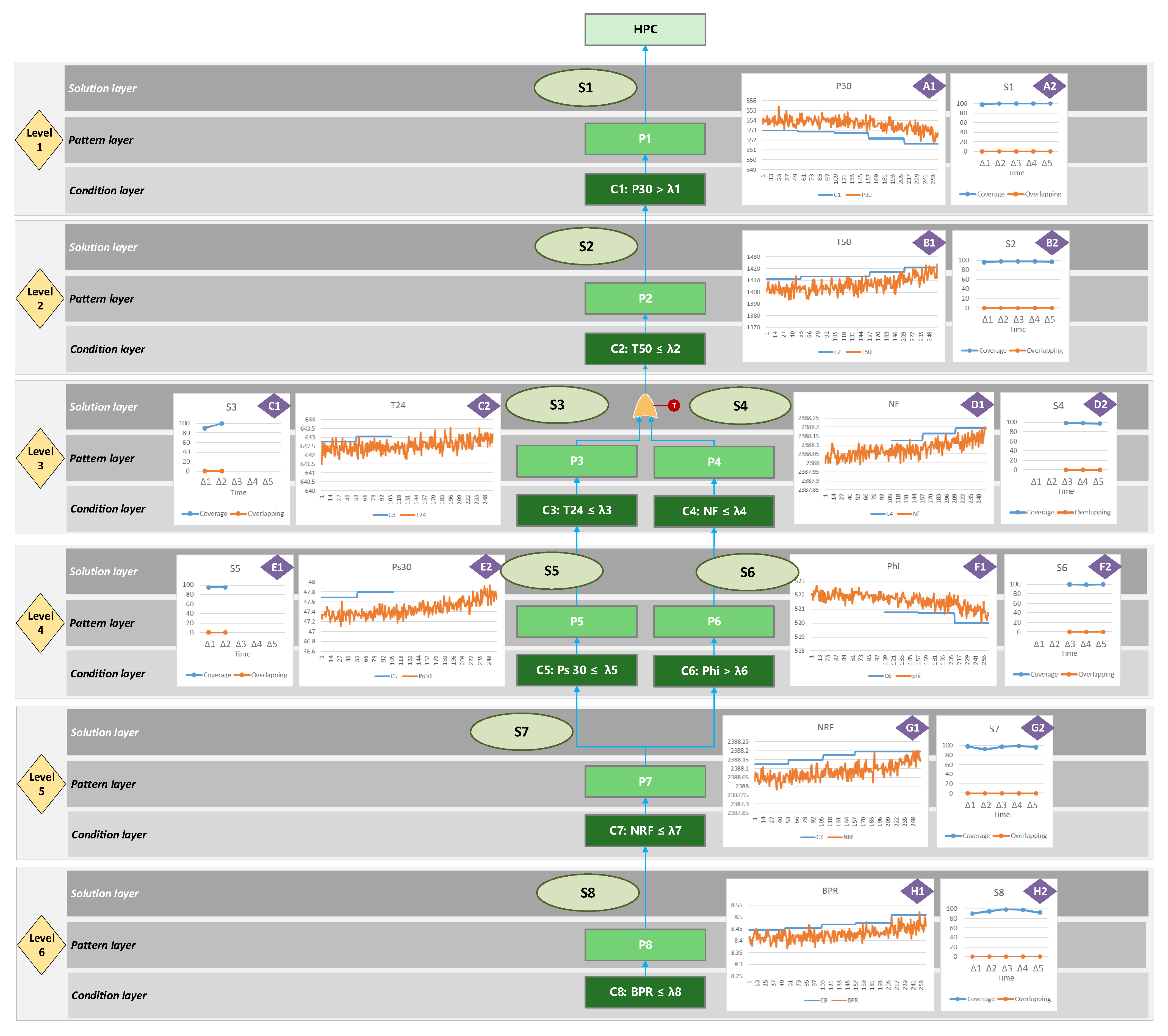
Figure 8 depicts the final ITCA model of the HPC fault mode. It includes six levels of decomposition to reproduce the causality structure between the HPC fault and its root-causes over six periods of time. Note that each level of the ITCA model consists of three layers that represent the solutions, patterns, and conditions related to the fault event or to one of its causes. The first level includes only one common feasible solution $S_1$ over the five defined time periods (${\mathsf{\Delta }}_1$ to ${\mathsf{\Delta }}_5$). $S_1$ has only one pattern, $P_1$, which includes only one condition: $C_1:P30>{\lambda }_1$. The plot A1 of Figure 8 characterizes the degradation of the variable P30 over time. Note that the cut-point curve (blue line) bounds the trend of the variable P30 in time. Additionally, the plot A2 of Figure 8 shows the common feasible solution coverage and the overlap percentages over the five time periods. Regarding Level 2 of the ITCA model, the same interpretation above can be performed for the variable T50. It is clear that the ITCA model captures the trend of the involved variables based on the cut-point curves.

At Level 3, two common feasible solutions, $S_3$ and $S_4$, are found by the time-based searching algorithm. These solutions respect the construction setting; $S_3$ explains the cause ($C_2: T50 \le {\lambda }_2$) at the time periods ${\mathsf{\Delta }}_1$ and ${\mathsf{\Delta }}_2$, while $S_4$ dominates the three other periods ${\mathsf{\Delta }}_3$ to ${\mathsf{\Delta }}_5$. $S_3$ and $S_4$ each have only one pattern and condition. The plots C2 and D1 of Figure 8 depict the bordering of the cut-point curves that represent the degradation trends of the variables T24 and NF, respectively. Meanwhile, the C1 and D2 plots show the solution coverage and overlap percentages over the corresponding time periods. $S_3$ and $S_4$ describe the full-time causality of the cause event ($C_2: T50 \le {\lambda }_2$) through the time–OR gate by toggling between the two feasible solutions. Hence, $S_3$ explains the event causality at only ${\mathsf{\Delta }}_1$ and ${\mathsf{\Delta }}_2$, while $S_4$ illustrates the causality of the same event at ${\mathsf{\Delta }}_3$, ${\mathsf{\Delta }}_4$, and ${\mathsf{\Delta }}_5$.

At Level 4, two other feasible solutions, $S_5$ and $S_6$, are found that explain the events $C_3: T24\le {\lambda }_3$) and $C_4: NF>{\lambda }_4$, respectively. At Level 5, only one common feasible solution $S_7$ is found that explains both events’ ($C_5: Ps30\le {\lambda }_5$ and $C_6: Phi\le {\lambda }_6$) causality over the five periods of time. This solution includes one pattern $P_7$ with only one condition $C_7:NRF\le {\lambda }_7$. The same reasoning can be made with the only common feasible solution $S_8,$ which explains the condition $C_7$ at the last level of the ITCA model using only one pattern $P_8$ that consists of one root cause: $C_8:BPR\le {\lambda }_8$. The cut-point curve of Figure 8. H1 bounds the trend of C₈.

From the obtained logic tree of Figure 8, the ITCA model confirms the discussion above about the main root cause of the HPC fault mode. Effectively, the first level of the ITCA model identifies the variable P30 (total pressure at HPC outlet) as the only fault indicator of the HPC degradation over time. Therefore, P30 can be employed to predict the remaining useful time of the turbofan engine according to the HPC fault mode. At the second level, the variable T50 (total temperature at an LPT outlet) is discovered to explain the effect of the temperature of combustion on the total pressure at the HPC outlet. T50 refines the knowledge discovered about P30. The same reasoning continues until reaching the final Level, 6, where the ITCA model discovers the variable BPR (bypass ratio), which is identified by the expert as the main control element that affects the occurrence of the HPC fault mode over time. Therefore, the ITCA model provides the expert with more refined knowledge, outlining the effects of the root causes on the fault trend over time, which help him to achieve the prognosis task in an efficient way.

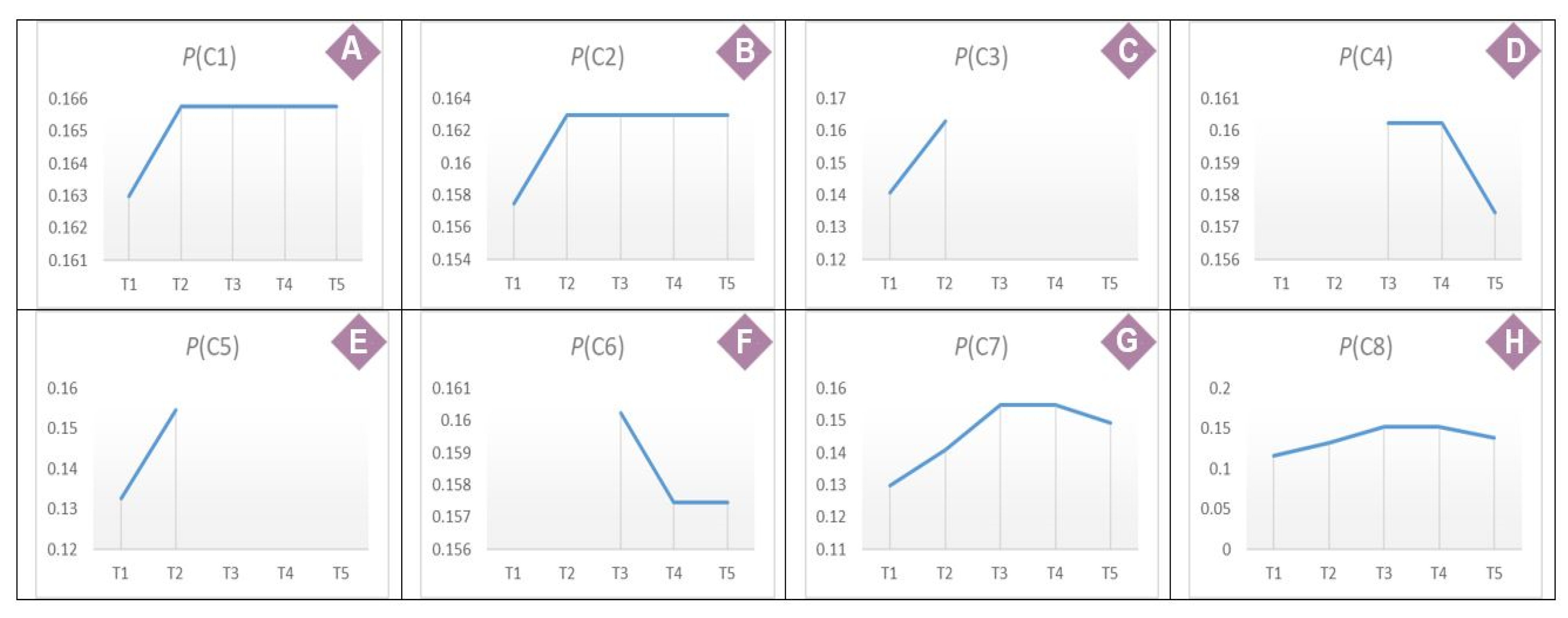
The probabilities associated with the ITCA model are calculated using Equations (1) to (4) of Stage 4, Phase 2. They quantify the occurrence of similar feasible solutions, patterns, and associated conditions, period after period, at each level of the ITAC model. Figure 9 plots the probabilities of the eight discovered conditions over five periods of time. Note that the occurrence of each feasible solution is equal to the probability of its associated conditions due to the structure of the obtained logic tree. For example, plot A in Figure 9 represents the probability curve of $S_1:P_1:C_1$ over the periods ${\mathsf{\Delta }}_1$ to ${\mathsf{\Delta }}_5$. The maximum probability value is equal to 0.16 at each period, since the original data are divided into six equal-size data subsets. Therefore, each subset represents 0.16 from the original data size. Note that each common feasible solution tries to maximize its class coverage, so that the associated condition probability value may not exceed that coverage value over the five periods.

Based on the ITCA model and the calculation of probabilities, only one time causality rule can be derived over five investigated periods, as follows:

$$\mathcal{P}\left(HPC\left({\mathsf{\Delta }}_i\right)\right)=\mathcal{P}\left(C_8\left({\mathsf{\Delta }}_i\right)\right) i=1\dots 5$$

(5)

The time causality rule expresses the contribution of the root-cause on the occurrence of the HPC fault, period after period, according to the $C_8$ cut-point curve. Each cut-point value provides the essential knowledge to sustain the turbofan for more or less time in each defined period interval through the maintenance action. For instance, the turbofan can spend more time in ${\mathsf{\Delta }}_1$ by making the $C_8$ variable (BPR) value under the corresponding cut-point value for a set of time.

4.3. Validation of the ITCA Model

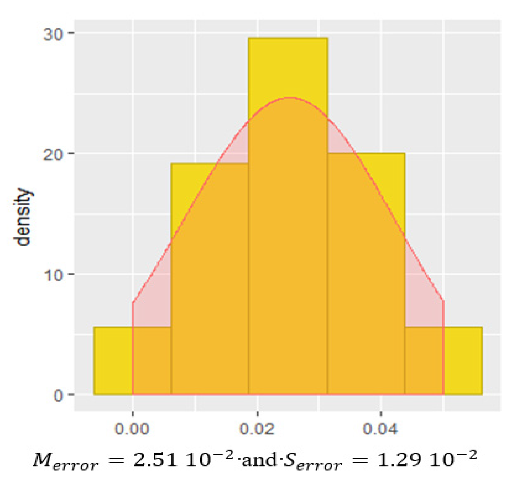
The accuracy of the obtained ITCA model is quantified using the testing dataset. Five concatenated datasets are formed to represent the five periods of time in the same manner as the data preparation of the training datasets. The mean and the standard error for each period are calculated using the time causality rule and 1000 random data samples; each has a size of 135 observations that provides a 95% confidence level, as shown in Figure 10. Based on the error in each period, an average error distribution is generated over the five periods.

From another point of view, the variables T2, P2, P15, epr, farB, Nf_dmd and PCNfR_dmd are not considered in the ITCA model of Figure 8 because they have a constant trend over time (see Table 1). However, the variables NC, NRc, htBleed, W31 and W32 have a changeable trend, but are not included in the ITCA model. To investigate this situation, the correlation matrix between those omitted variables and those already considered in the ITCA model are measured, as depicted in

Table 2. Correlation matrix. The bold cell shows the maximum correlation value.

	NC	NRc	htBleed	W31	W32
T24	−0.159	−0.502	0.595	−0.629	−0.614
T30	−0.211	−0.459	0.534	−0.543	−0.582
T50	−0.153	−0.548	0.644	−0.727	−0.699
P15	−0.001	−0.014	0.065	−0.059	−0.107
P30	0.175	0.588	−0.651	0.718	0.739
Nf	−0.167	−0.594	0.707	−0.750	−0.743
Ps30	−0.171	−0.594	0.689	−0.761	−0.742
phi	0.158	0.616	−0.688	0.722	0.721
NRf	−0.169	−0.582	0.708	−0.746	−0.715
BPR	−0.184	−0.575	0.605	−0.663	−0.714

. In each column, the bold value shows the maximum correlation value. The variables NRc, htBleed, and both W31 and W32 are correlated to the variables phi, Nrf and Ps30, respectively, with a correlation value that is higher than 0.6. Except for the variable NC, which measures the physical core speed, and is correlated to P30 with the highest absolute value of 0.17. Accordingly, it seems to be relevant for the HPC degradation. This could be overlooked by the ITCA model.

5. Conclusions

This paper has proposed an interpretable time causality analysis (ITCA) methodology for aging systems. The ITCA model represents the fault hierarchy causality by using the logic of the graphical fault tree and the knowledge discovery in the dataset. The obtained tree models the effect of the system’s aging on the changes in the fault causality structure over time to better achieve fault prognosis. The illustrated case study demonstrates its usefulness and ability to discover only the relevant root cause that impacts the fault behaviour. Based on the model’s interpretability, the expert is able to use the time causality structure of the turbofan HPC degradant performance to support his decision. Thus, the ITCA model provides the expert with the deep causality knowledge that explains the fault evolution over time. Unlocking the data-driven model’s complexity by providing an interpretable graphical model, in addition to summarizing the evolution of the fault over time in one interpretable model are the two major contributions of the ITCA model over the current time causality data-driven models for fault prognosis. The ITCA model takes a further step towards reinforcing the link between experts and data-driven models. Such a model will help experts elucidate and implement the maintenance decision-making process.

Our next research work will be to assist the expert by better optimizing the system performance through a set of control actions to maximize the RUL. We hope to allow our future ITCA model to demonstrate the system’s reaction regarding a set of proposed control actions based on its causality rules and link the impact of a given proposed action to the RUL. The expert still needs to observe this system’s reaction, represented by the new fault causality structure that reflects the system’s response to the causality rule control actions that are taken, and note how this improves the RUL. Therefore, the future ITCA model must include different scenarios for fault causality structures that reflect the impact of the different combinations of control actions based on the derived causality rules.

References

1. Vogl, G.W.; Weiss, B.A.; Helu, M. A review of diagnostic and prognostic capabilities and best practices for manufacturing. J. Intell.Manuf. 2019, 30, 79–95. [Google Scholar] [CrossRef] [PubMed]
2. Ming, L.; Yan, H.-C.; Hu, B.; Zhou, J.-H.; Pang, C.K. A data-driven two-stage maintenance framework for degradation prediction in semiconductor manufacturing industries. Comput. Ind. Eng. 2015, 85, 414–422. [Google Scholar]
3. de Jonge, B. Discretizing continuous-time continuous-state deterioration processes, with an application to condition-based maintenance optimization. Reliab. Eng. Syst. Saf. 2019, 188, 1–5. [Google Scholar] [CrossRef]
4. Gao, Z.; Cecati, C.; Ding, S.X. A survey of fault diagnosis and fault-tolerant techniques—Part I: Fault diagnosis with model-based and signal-based approaches. IEEE Trans. Ind. Electron. 2015, 62, 3757–3767. [Google Scholar] [CrossRef] [Green Version]
5. Wang, K.S. Key techniques in intelligent predictive maintenance (IPdM)—A framework of intelligent faults diagnosis and prognosis system (IFDaPS). In Proceedings of the 4th International Workshop of Advanced Manufacturing and Automation (IWAMA 2014), Shanghai, China, 27–28 October 2014. [Google Scholar]
6. Bousdekis, A.; Magoutas, B.; Apostolou, D.; Mentzas, G. Review, analysis and synthesis of prognostic-based decision support methods for condition based maintenance. J. Intell. Manuf. 2018, 29, 1303–1316. [Google Scholar] [CrossRef]
7. Schwabacher, M.A. A survey of data-driven prognostics. In Proceedings of the Infotech@ Aerospace 2005, Arlington, VA, USA, 26–29 September 2005; p. 7002. [Google Scholar]
8. Aggab, T.; Kratz, F.; Avila, M.; Vrignat, P. Model-based prognosis applied to a coupled four tank MIMO system. IFAC PapersOnline 2018, 51, 655–661. [Google Scholar] [CrossRef]
9. Schwabacher, M.; Goebel, K. A survey of artificial intelligence for prognostics. In Proceedings of the Artificial Intelligence for Prognostics—Papers from the AAAI Fall Symposium, Arlington, VA, USA, 9–11 November 2007. [Google Scholar]
10. Waghen, K.; Ouali, M.-S. Interpretable logic tree analysis: A data-driven fault tree methodology for causality analysis. Expert Syst. Appl. 2019, 136, 376–391. [Google Scholar] [CrossRef]
11. Chen, H.-S.; Yan, Z.; Zhang, X.; Liu, Y.; Yao, Y. Root Cause Diagnosis of Process Faults Using Conditional Granger Causality Analysis and Maximum Spanning Tree. IFAC PapersOnLine 2018, 51, 381–386. [Google Scholar] [CrossRef]
12. Vania, A.; Pennacchi, P.; Chatterton, S. Fault diagnosis and prognosis in rotating machines carried out by means of model-based methods: A case study. In Proceedings of the ASME 2013 International Design Engineering Technical Conferences and Computers and Information in Engineering Conference, IDETC/CIE 2013, Portland, OR, USA, 4–7 August 2013. [Google Scholar]
13. Lu, N.; Jiang, B.; Wang, L.; Lü, J.; Chen, X. A Fault Prognosis Strategy Based on Time-Delayed Digraph Model and Principal Component Analysis. Math. Probl. Eng. 2012, 2012, 937196. [Google Scholar] [CrossRef]
14. Darwish, M.; Almouahed, S.; de Lamotte, F. The integration of expert-defined importance factors to enrich Bayesian Fault Tree Analysis. Reliab. Eng. Syst. Saf. 2017, 162, 81–90. [Google Scholar] [CrossRef]
15. Ragab, A.; El Koujok, M.; Ghezzaz, H.; Amazouz, M.; Ouali, M.-S.; Yacout, S. Deep understanding in industrial processes by complementing human expertise with interpretable patterns of machine learning. Expert Syst. Appl. 2019, 122, 388–405. [Google Scholar] [CrossRef]
16. Yunkai, W.; Jiang, B.; Lu, N.; Zhou, Y. Bayesian Network Based Fault Prognosis via Bond Graph Modeling of High-Speed Railway Traction Device. Math. Probl. Eng. 2015, 2015, 321872. [Google Scholar]
17. Jin, S.; Zhang, Z.; Chakrabarty, K.; Gu, X. Failure prediction based on anomaly detection for complex core routers. In Proceedings of the 37th IEEE/ACM International Conference on Computer-Aided Design, ICCAD 2018, San Diego, CA, USA, 5–8 November 2018. [Google Scholar]
18. Niu, G. Data-Driven Technology for Engineering Systems Health Management: Design Approach, Feature Construction, Fault Diagnosis, Prognosis, Fusion and Decisions; Springer: Singapore, 2016; pp. 1–357. [Google Scholar]
19. Zhang, Z.; Wang, Y.; Wang, K. Fault diagnosis and prognosis using wavelet packet decomposition, Fourier transform and artificial neural network. J. Intell. Manuf. 2013, 24, 1213–1227. [Google Scholar] [CrossRef]
20. Wu, Q.; Ding, K.; Huang, B. Approach for fault prognosis using recurrent neural network. J. Intell. Manuf. 2020, 31, 1621–1633. [Google Scholar] [CrossRef]
21. Razavi, S.A.; Najafabadi, T.A.; Mahmoodian, A. Remaining Useful Life Estimation Using ANFIS Algorithm: A Data-Driven Approcah for Prognostics. In Proceedings of the 2018 Prognostics and System Health Management Conference, PHM-Chongqing 2018, Chongqing, China, 26–28 October 2018. [Google Scholar]
22. Doukovska, L.; Vassileva, S. Knowledge-based Mill Fan System Technical Condition Prognosis. WSEAS Trans. Syst. 2013, 12, 398–408. [Google Scholar]
23. Li, Z.; Wang, Y.; Wang, K. A data-driven method based on deep belief networks for backlash error prediction in machining centers. J. Intell. Manuf. 2020, 31, 1693–1705. [Google Scholar] [CrossRef]
24. Su, Y.; Jing, B.; Huang, Y.-F.; Tang, W.; Wei, F.; Qiang, X.-Q. Correlation analysis method between environment and failure based on fuzzy causality diagram and rough set of multiple decision classes. Instrum. Tech. Sens. 2015, 100–103. [Google Scholar]
25. Kimotho, J.K.; Sondermann-Woelke, C.; Meyer, T.; Sextro, W. Application of Event Based Decision Tree and Ensemble of Data Driven Methods for Maintenance Action Recommendation. Int. J. Progn. Health Manag. 2013, 4 (Suppl. S2), 1–6. [Google Scholar] [CrossRef]
26. Medjaher, K.; Moya, J.Y.; Zerhouni, N. Failure prognostic by using Dynamic Bayesian Networks. IFAC Proc. Vol. 2009, 42, 257–262. [Google Scholar] [CrossRef] [Green Version]
27. Hammer, P.L.; Bonates, T.O. Logical analysis of data—An overview: From combinatorial optimization to medical applications. Ann. Oper. Res. 2006, 148, 203–225. [Google Scholar] [CrossRef]
28. Fokkema, M. PRE: An R package for fitting prediction rule ensembles. arXiv 2017, arXiv:1707.07149. [Google Scholar] [CrossRef] [Green Version]
29. May, R.; Csank, J.; Litt, J.; Guo, T.-H. Commercial Modular Aero-Propulsion System Simulation 40k (C-MAPSS40k) User’s Guide. NASA TM-216831. 2010. Available online: https://www.researchgate.net/publication/273755967_Commercial_Modular_Aero-Propulsion_System_Simulation_40k_C-MAPSS40k_User’s_Guide (accessed on 30 September 2021).
30. Frederick, D.K.; de Castro, J.A.; Litt, J.S. User’s Guide for the Commercial Modular Aero-Propulsion System Simulation (C-MAPSS): Version 2. 2012. Available online: https://ntrs.nasa.gov/citations/20120003211 (accessed on 30 September 2021).
31. National Aeronautics and Space Administration NASA. Turbofan Engine. 2015. Available online: https://www.grc.nasa.gov/www/k-12/airplane/Animation/turbtyp/etfh.html (accessed on 30 September 2021).
32. Frederick, D.K.; de Castro, J.A.; Litt, J.S. User’s Guide for the Commercial Modular Aero-Propulsion System Simulation (C-MAPSS). 2007. Available online: https://ntrs.nasa.gov/citations/20070034949 (accessed on 30 September 2021).
Figure 1. The four-phase ITCA methodology.
Algorithms 15 00178 g001
Figure 2. Data preparation phase.
Algorithms 15 00178 g002
Figure 3. Example of selecting similar feasible solutions over the periods Δ1, Δ2, and Δ3.
Algorithms 15 00178 g003
Figure 4. Curve of the cut-point values of similar feasible solutions obtained over time.
Algorithms 15 00178 g004
Figure 5. Time–OR gate functionality in the ITCA model.
Algorithms 15 00178 g005
Figure 6. Generating new labelled data subsets in the ITCA methodology.
Algorithms 15 00178 g006
Figure 7. The simulated turbofan engine based on C-MAPSS [32] (images courtesy of NASA). (A) Simplified diagram of the turbofan engine; (B) Turbofan engine modules layout and connections.
Algorithms 15 00178 g007
Figure 8. Obtained ITCA model of the HPC degradation mode.
Algorithms 15 00178 g008
Figure 9. Probability calculations of the HPC fault mode.
Algorithms 15 00178 g009
Figure 10. Accuracy of the ITCA model.
Algorithms 15 00178 g010