Cicada Species Recognition Based on Acoustic Signals

Abstract

Traditional methods used to identify and monitor insect species are time-consuming, costly, and fully dependent on the observer’s ability. This paper presents a deep learning-based cicada species recognition system using acoustic signals to classify the cicada species. The sound recordings of cicada species were collected from different online sources and pre-processed using denoising algorithms. An improved Härmä syllable segmentation method is introduced to segment the audio signals into syllables since the syllables play a key role in identifying the cicada species. After that, a visual representation of the audio signal was obtained using a spectrogram, which was fed to a convolutional neural network (CNN) to perform classification. The experimental results validated the robustness of the proposed method by achieving accuracies ranging from 66.67% to 100%.

1. Introduction

The 17-year periodical cicadas are cicada species with life cycles as long as 17 years. These cicada species spend most of their lifetime underground and only emerge from the ground once every 17 years to reproduce before dying in four to six weeks. Coming from the singing insect family, cicada species emit sounds that are species-specific for communication purposes [1]. Male cicadas can produce deafening clicking sounds with frequencies up to 7 kHz at a 100 dB sound pressure level [2]. Their sounds are produced from the vibration of drum-like membranes, called timbals, which can be found on both sides of their body [3,4]. Female cicadas, on the other hand, produce a less loud sound using their wings to respond to the male’s calling.

For a long time, detecting and classifying cicada species have been conducted by numerous researchers. There are mainly two approaches for this task. The first one is based on traditional method where the type of cicada species is determined by the domain experts manually. This process is time-consuming, costly, and dependent on the observer’s ability. Following the advancement of technology, researchers have utilized machine learning algorithms to develop systems for cicada species identification and classification. In general, cicada species recognition systems can be created using two sources: (1) visual images of the cicadas, and (2) species-specific acoustic signals emitted by cicadas. However, under conditions where the visual images are not clear or for cicadas that live in complex environments, acoustic signals are a more favorable source than images.

From the study on related works, it was found that the current research is more inclined to use conventional methods, such as support vector machine (SVM) and random forest (RF), to build the classification model instead of deep learning methods that can be more effective [5]. Therefore, we propose to develop a cicada species recognition system using a deep learning algorithm. With the use of a deep learning-based cicada species recognition system, monitoring of cicada species can be carried out more efficiently in terms of time and effort. Three 17-year periodical cicada species were selected for the acoustic signal recognition task, namely Magicicada cassinii, Magicicada septendecim, and Magicicada septendecula. Audio recordings of their different sound types such as calling and courtship sounds were collected.

This paper is organized in the following order. Section 2 presents the study on related works. Section 3 details the methods used and the proposed solution for cicada species detection and classification, while Section 4 shows the experimental results. Section 5 summarizes the important findings in the experiments, and lastly, Section 6 provides the conclusion and future works.

2. Related Works

Throughout the years, various research have been conducted on insect or animal detection and classification using their acoustic signals. Generally, the sound recognition process involves two stages, namely feature extraction and classification, while the segmentation of audio signals may sometimes be applied depending on the dataset. The species of study vary from one research to another, such as cicadas, crickets, bees, birds, and more.

2.1. Conventional Methods

Before deep learning methods became increasingly common, researchers focused on using conventional methods, such as support vector machine (SVM) and random forests (RF), for insect or animal detection and classification. The performances of conventional methods are dependent on the feature extraction process to obtain high performance in terms of classification accuracy [6].

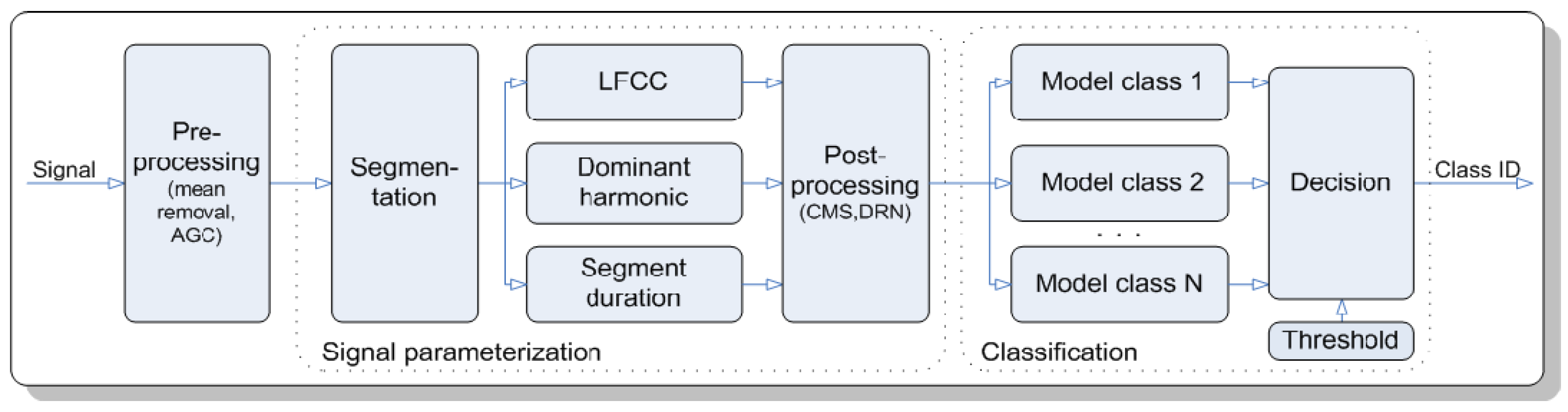
In 2007, Potamitis, Ganchev, and Fakotakis [7] attempted to classify species of crickets and cicadas using their acoustic signals with a probabilistic neural network (PNN) and Gaussian mixture models (GMM). The dataset consists of audio recordings of 220 species of crickets and cicadas obtained from the Singing Insects of North America (SINA) collection. The recognition process has two main stages, which are signal parameterization and classification. Figure 1 shows the detailed steps of the acoustic insect recognition process. This experiment obtained a high accuracy of 99% and above for classifications at levels of singing insect and family and 90% for classification at species level using the fusion of PNN and GMM. However, the identification accuracy of this fusion was found to be insufficient for practical applications despite the performance gain.

Figure 1. Diagram of the acoustic insect recognition process for N classes [5].

In 2010, Zhu and Zhang [8] conducted research to identify different sounds of insects automatically with the aim of providing convenience for technicians in pest management. A total of 50 different insect sounds were collected from the insect sound library from the Agricultural Research Service (ARS) of the United States Department of Agriculture (USDA). This experiment classifies these insect sounds according to their sound types, such as “movement and feeding sounds of soil invertebrates”, “defensive stridulation of soil insects”, “wind and abdominal vibration sounds”, etc. To extract the features of the insect sounds, sub-band-based cepstral (SBC) was used, while a Hidden Markov Model (HMM) was used for classification. The experiment achieved a high classification accuracy of 90.98%. As the dataset used in this research was selected from noise-free sections of the recorded signal, the model may not work well with insect sounds with a noisy background.

In 2019, research on the automated classification of bee species and hornet species using acoustic analysis was conducted by Kawatika and Ichikawa [9]. Through this research, they aimed to monitor predator-prey relationships that can contribute to the ecological domain. The species chosen for the experiment were three honey-bee species and a hornet. The datasets used were self-recorded in rural areas and remote forests in Japan. To extract the feature values of the signals, MFCC was used, while SVM was used for classification. The experiment succeeded with high recall and precision of 0.96 to 1.00 in distinguishing bees and hornets from the environment and relatively high recalls and precision of 0.7 to 1.0 in identifying bees and hornets at the species level. Despite the high performances obtained, the model faces difficulties in classifying species with subtle differences in their sound features.

Furthermore, in the same year, Noda et al. [1] conducted experiments to identify 343 species of crickets, katydids, and cicadas by analyzing their acoustic signals. Out of the 343 species dataset, sound recordings of 255 species of crickets, katydids, and cicadas were obtained from the SINA collection, while sound recordings of the remaining 88 species of cicadas were retrieved from the Insect Singers corpora. In this research, they have proposed a new sound parameterization technique, a fusion between MFCC and LFCC, to represent the sounds of insects more effectively. As for the classification method, SVM and RF algorithms were used. Experiments were carried out using different combinations of feature extraction methods, MFCC, LFCC, and MFCC/LFCC fusion, and classifiers, SVM and RF, to obtain the best result. At the end of the experiment, a high accuracy rate of 98.07% was obtained when classifying 343 species of crickets, katydids, and cicadas at the species level using MFCC/LFCC fusion and SVM. However, similar to previous studies, this model has a limitation in identifying insect species with similar frequency ranges.

Recently, in February 2022, Marugaiya, Abas, and De Silva [10] proposed classifying the sound of bird species using Gammatone frequency cepstral coefficient (GTCC) and Probability Enhanced Entropy (PEE) for feature extraction, using SVM as the classifier. The dataset used in this experiment consisted of 20 Bornean bird species collected from the Xeno-canto database. Initially, the audio recordings were segmented using automated energy-based segmentation. Then, features were extracted from the audio segments using GTCC and the resulting feature matrix was passed to the SVM classifier for training and classification. The overall accuracy obtained from these settings was 81%. The authors found that the original GTCC method does not fit the wide frequency range of the bird sounds, and thus, the GTCC filter bank range was modified. The experiment was repeated using the improved GTCC and a combination of improved GTCC and PEE for feature extraction to further improve the classification accuracy. At the end of the experiments, the SVM model achieved a higher overall accuracy of 86% and 89.5% when using the improved GTCC and GTCC + PEE, respectively. Moreover, the species-level accuracy of the 20 bird species fluctuates within a range of 70% to 100%.

2.2. Deep Learning Methods

Following the advancement and success of deep learning models in image processing, researchers have started to explore more possibilities of this powerful architecture by using it for acoustic signal recognition. The basic idea of this process is to visualize the acoustic signals or extracting the features of the signals, similar to conventional methods, and pass it to the model for classification. The use of deep learning methods has also become increasingly popular in insect detection and classification as more studies are conducted on insect acoustic analysis using deep learning models, such as multilayer perceptron (MLP) and convolutional neural network (CNN).

As early as 2004, Chesmore [11] developed a model to identify four species of grasshopper using their bioacoustics signals in a noisy environment. The dataset was self-recorded by the researcher at various sites and habitats of the species in England. Time Domain Signal Coding (TDSC) and MLP were used in this experiment. A total of 13 sound sources were used to train the model, which includes sounds of four grasshopper species, birds, vehicles, and more. The experiments achieved an overall high accuracy of 81.8% to 100% in classifying four grasshopper species from the 13 sound sources when a threshold of 0.9 was applied to remove classification results below the threshold. Additionally, this model was also able to identify the sounds of a grasshopper species, a light aircraft, and a bird alarm call from a sound recording, which shows its potential in general sound mapping applications.

In 2017, Zamaniam and Pourghassem [12] proposed to use an MLP classifier to classify five cicada species based on the spectral and temporal features of their sound. The dataset used in this experiment was self-recorded by the researchers in the natural environment in Iran, and only the calling songs of the cicada species were selected. Levenberg Marquardt (LM) was chosen as the training algorithm. At the end of the experiment, high accuracy of 96.70% was achieved when all features were weighted. The model was further improved by applying a genetic algorithm for feature selection and obtained a higher accuracy rate of 99.13%. Given the outstanding classification rate, the researchers are confident that the model proposed not only can be used to classify cicada species but is applicable for the classification of other insect species as well. A downside of this study is that the scope is limited to classifying cicada species based on their calling songs only, yet cicada species produce other sounds to communicate, including courtship and distress sounds.

Moreover, in 2018, Dong, Yan, and Wei [13] introduced an approach for insect recognition using enhanced spectrograms and CNN. The dataset used consists of sound recordings of 47 insect species retrieved from the sound library of ARS of USDA. The spectrogram images were generated in MATLAB and enhanced using contrast-limit adaptive histogram equalization (CLAHE) to reduce noise. The resulting enhanced spectrograms were two-dimensional grey images, and the images were directly passed to the CNN model for classification. The experiment succeeded with a high average accuracy rate of 97.8723%, and it is said to be the highest accuracy obtained among past studies conducted on the same dataset. However, since the model has not been used upon large scale datasets, it remains unknown whether the performance of the model persists if tested.

In early 2021, Arpitha, Kavya Rani, and Lavanya [14] proposed a model to classify four mosquito species based on the sound of their wingbeats. The dataset used was obtained from the Kaggle repository, which consists of 1200 samples of mosquito wingbeat sounds. The signals were pre-processed by framing using Hamming window function and feature scaling using an octave scale. This experiment proposed to develop a CNN model with unsupervised transfer learning strategies. A residual-network-50 (ResNet-50) was built, and the model was validated using the KFold Validation technique. The experiment achieved a high overall accuracy of 96% for classifying four mosquito species. With high performance, this model was said to be useful for other sound classification applications, such as bird species recognition, after applying some modifications. The limitation of this research is that the number of classes used in the experiment was few.

Later, in November 2021, Zhang et al. [15] introduced an approach to classify insect sounds using MFCC for feature extraction and CNN for classification. The dataset was obtained from the sound library of ARS, USDA, the same as previous experiments. Since the audio recordings in the dataset varied in audio length, longer recordings were taken as the training dataset, while the shorter ones were used as the testing dataset. The dataset was pre-processed by normalization and pre-emphasis before applying MFCC for feature extraction. The resulting feature maps were passed as input to the CNN model for training and classification. The model will classify the sounds based on their sound types (nine classes). At the end of the experiment, the model achieved an average classification rate of 92.56%. However, some classes achieved a low class-wise accuracy of 69% due to the low number of samples available.

3. Materials and Methods

In this section, the details of the cicada species recognition system are discussed. The audio signals of the cicada species were first pre-processed. After that, the Härmä syllable segmentation (Härmä) algorithm was implemented to segment the audio signals according to syllables. Next, the processed audio signals were visualized in the form of a spectrogram. Then, a deep learning model was developed for training and classification.

3.1. Proposed Cicada Species Recognition using Acoustic Signals

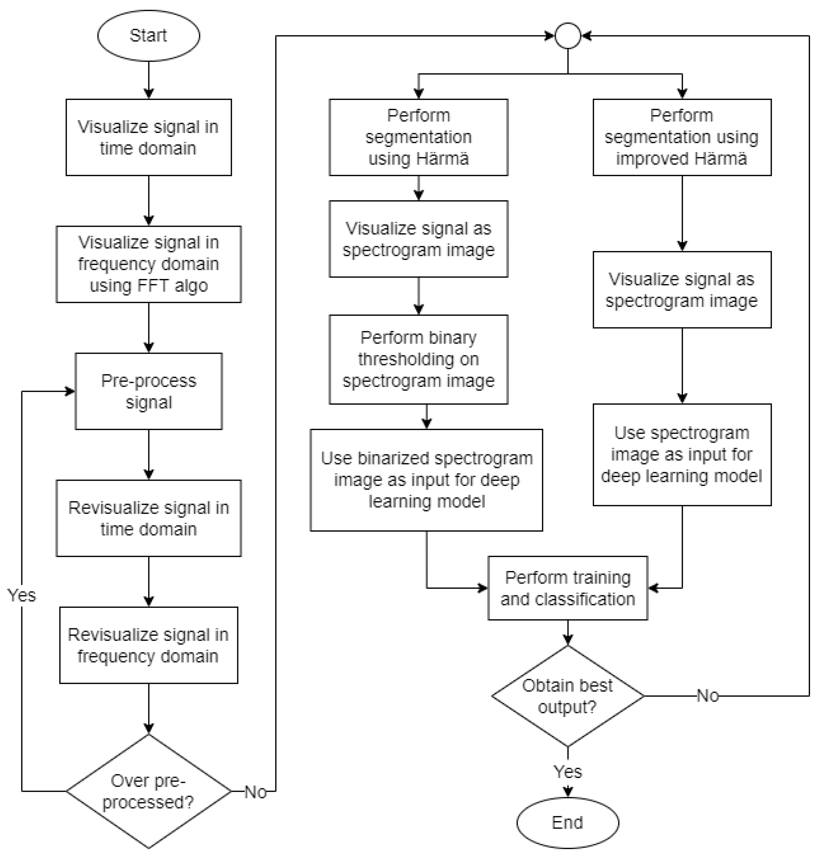
Figure 2 illustrates the overall process flow involved in the proposed cicada species recognition system. Generally, the processes involved are pre-processing, segmentation, visualization of signal, and lastly, training and classification. Detailed descriptions of each process are presented in the following sections.

Figure 2. Flowchart of the proposed cicada species recognition system.

First, the audio signals were visualized in the time domain by plotting a graph of the amplitude of signal against time. This is to observe the signal pattern and have a basic understanding of the sound of cicada species. Next, the audio signals were visualized in the frequency domain using the Fast Fourier Transform (FFT) algorithm [16]. A graph of the magnitude against the frequency of the signal was plotted for each audio signal to analyze the frequency range of the signal and to identify the frequencies with high magnitudes.

Then, the audio signals were pre-processed to remove the background noises by denoising. The pre-processed signals were revisualized in the time domain as well as the frequency domain to observe the changes in the signals. If the graphs of the signals show signs of over pre-processing, the signals will be pre-processed again.

Subsequently, audio segmentation was applied to the pre-processed signals using the Härmä syllable segmentation (Härmä) algorithm. The Härmä algorithm segmented out the syllables from the original signal to remove noise and unwanted signals. Since the algorithm segmented out the important syllables from the original signal based on their time values, each segment still contained low-amplitude signals that were not significant to the training process. Thus, to solve this problem, binary thresholding was applied to remove unnecessary information from the spectrogram images generated from the signal after applying the Härmä algorithm. Alternatively, we also present an improved Härmä algorithm that removes low-amplitude signals during the segmentation process so that binary thresholding is not required.

After that, the signals were converted to spectrogram representation to be passed as input to the deep learning model to perform training and classification. Two sets of spectrogram images processed in different ways, namely binarized spectrograms and the spectrograms obtained from the improved Härmä algorithms, were trained separately, and the performances of the models were evaluated. We checked if the model obtained the best output, i.e., obtained a high classification accuracy without overfitting, and made some modifications if the output was not satisfactory.

3.2. Software

In this paper, MATLAB was used to generate spectrogram representations for the acoustic signals of the cicada species. The built-in functions, Signal Processing Toolbox and Härmä syllable segmentation were implemented in this paper and eased the entire development process.

The software used to pre-process the signals, binarize the spectrograms, and build the classification model was Google Colaboratory. The signals were pre-processed using scipy.signal.butter or Butterworth filter from SciPy library, while the spectrograms were binarized using cv2.threshold from OpenCV library. The classification model was built using Keras API from TensorFlow.

3.3. Dataset

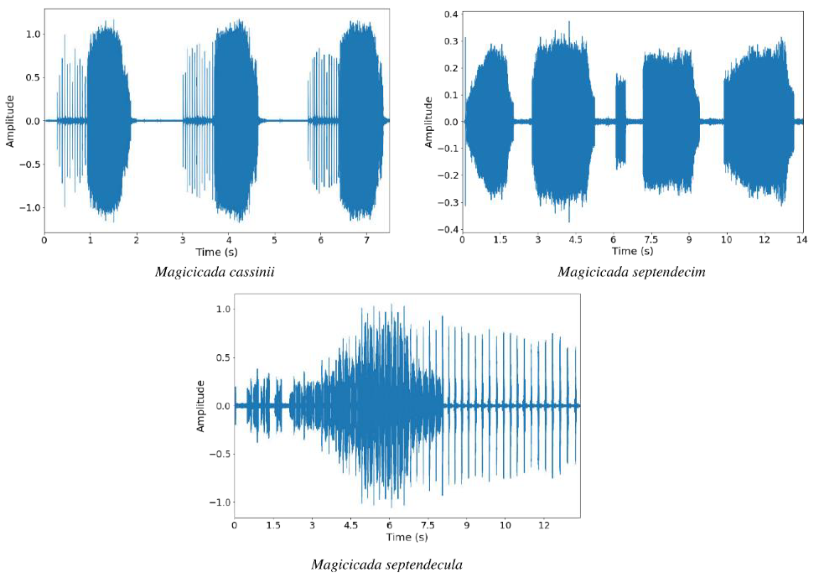
The dataset used in this experiment was collected from various online sources, such as Freesound and other websites. There is no readily available dataset for cicada species. The dataset consists of a total of 43 sound recordings of three different cicada species, namely Magicicada cassinii, Magicicada septendecim, and Magicicada septendecula. The Magicicada cassinii and Magicicada septendecula species each has 14 audio files while Magicicada septendecim has 15 audio files. All sound recordings were recorded in mono at a sampling rate of 44.1 kHz. 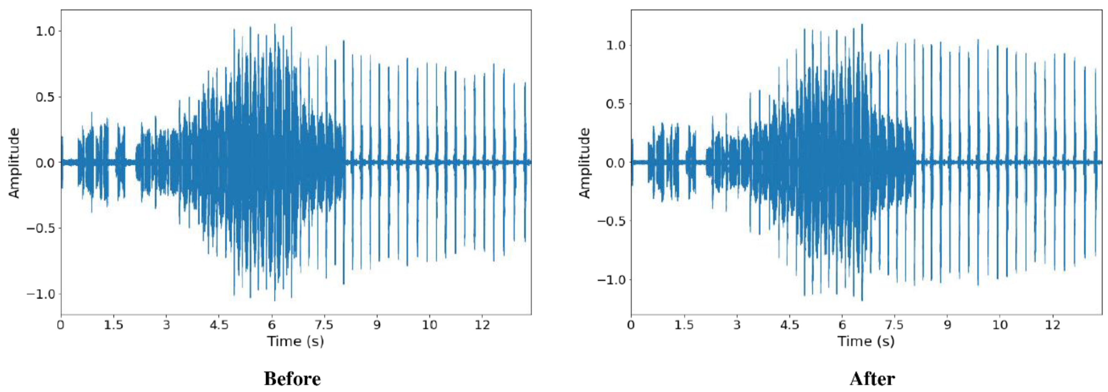Figure 3 shows some samples of the waveform of sounds of each species, while Table 1 shows the details of the audio recordings used in this paper.

Figure 3. Waveform visualization of sounds of each species.

Table 1. Details of audio recordings.

Species	No. of Recordings	Length of Recordings	Total Active Calling (min)	No. of Syllables from Each Recording (Average)
				Härmä	Improved Härmä
Magicicada cassinii	14	7 s–1 min	4.60	21	10
Magicicada septendecim	15	3–37 s	3.85	12	2
Magicicada septendecula	14	5–50 s	5.27	14	3

3.4. Pre-Processing

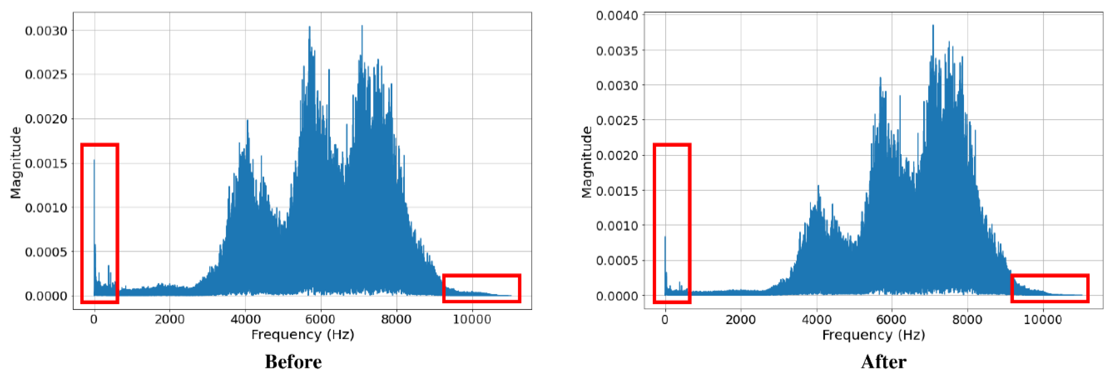
The dataset was pre-processed by denoising the audio signals using the Butterworth filter. Both high pass and low pass filters were applied to the audio signals. The low pass filter was applied with a cut-off point at 10 kHz, while the high pass filter was applied with a cut-off point at 1 kHz. After denoising, the noises with frequencies above 10 kHz and below 1 kHz were mostly removed from the audio recording (Figure 4).

Figure 4. Frequency domain of signals before and after pre-processing.

From Figure 4 and Figure 5, we also observed that the signals, before and after pre-processing, do not differ much in peak frequency, syllable length, and syllable repetition rate, which shows its potential to be applied in the actual environment.

Figure 5. Time domain of signals before and after pre-processing.

3.5. Audio Segmentation

3.5.1. Härmä Syllable Segmentation Algorithm

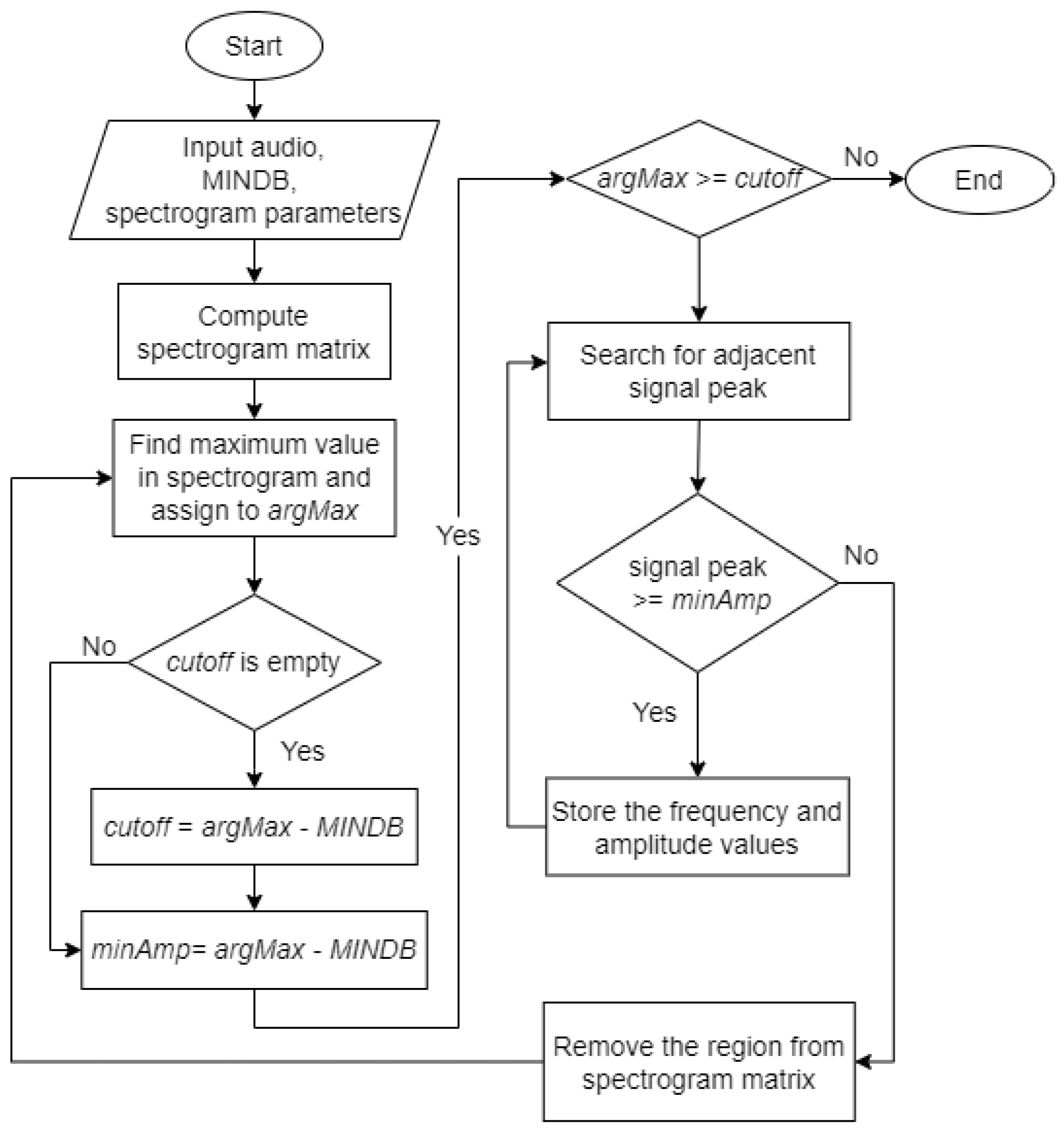
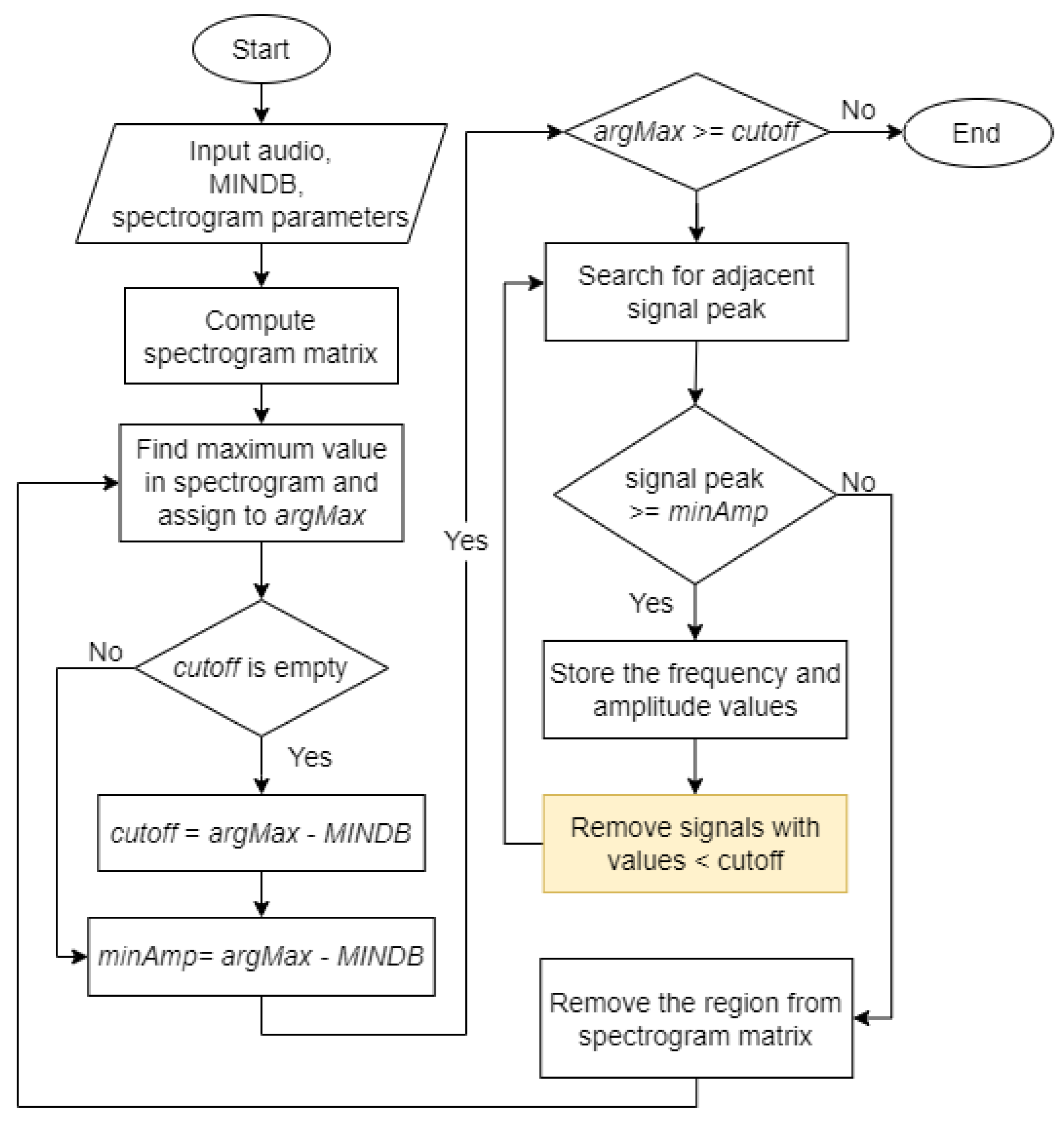
The Härmä syllable segmentation (Härmä) algorithm was introduced by Härmä [17]. Figure 6 shows the flowchart for the Härmä algorithm. Initially, the pre-processed audio signal was passed to the algorithm along with a value of the stopping criteria, MINDB, in decibels and the parameters required to generate a spectrogram matrix, which are sampling frequency, window size, overlap size, and Fast Fourier Transform (FFT) size.

Figure 6. Flowchart of the Härmä syllable segmentation algorithm.

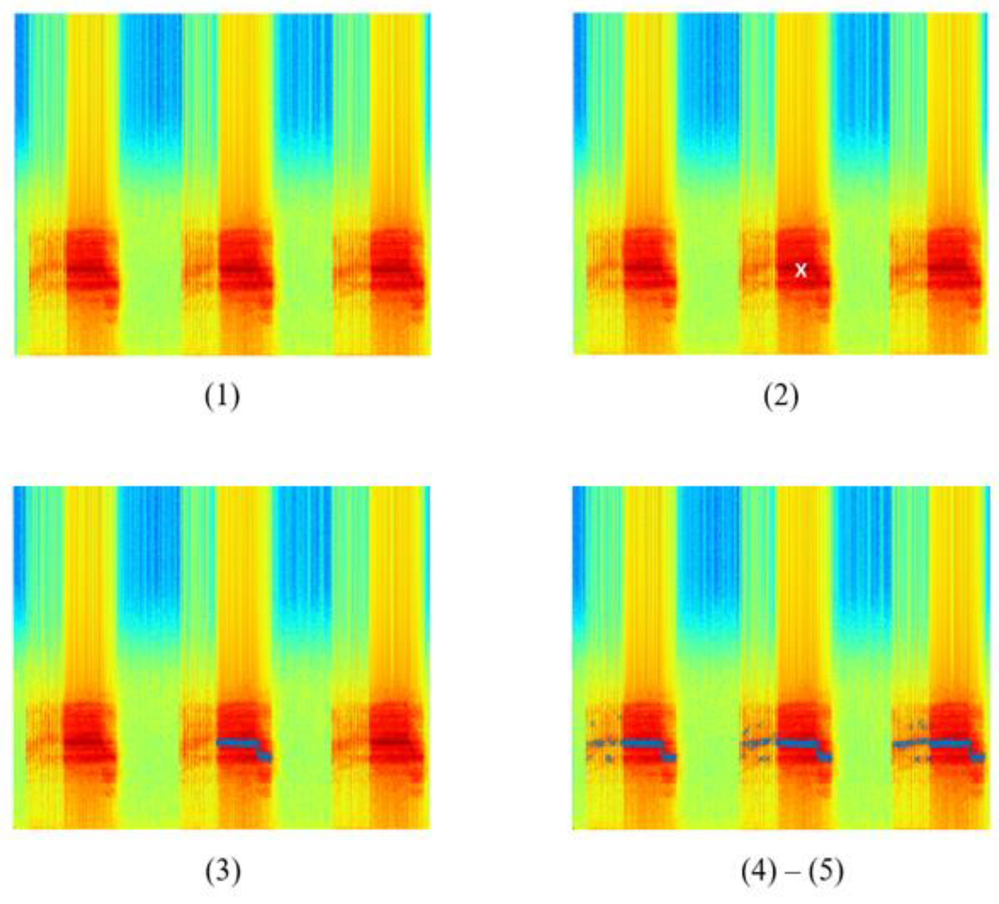
The output of each step involved in the Härmä algorithm is shown in Figure 7. The spectrogram images are for illustration purposes only. Only one spectrogram image will be generated upon complete execution of the algorithm.

Figure 7. Output of steps involved in the Härmä syllable segmentation algorithm.

The algorithm generated a spectrogram matrix, $S\left(f, t\right)$, from the input audio.

The algorithm finds the maximum value, $\left|S\left(f_n, t_n\right)\right|$, in the spectrogram matrix and converts the value to decibels before assigning to the variable $argMax$ defined in (1).

$$argMax=20 lo{g}_{10}\left| S\left(f_n, t_n\right)\right|$$

(1)

In the first iteration, the algorithm defined $cutoff$ as (2) and $minAmp$ as (3).

$$cutoff=argMax-MINDB$$

(2)

$$minAmp=argMax-MINDB$$

(3)

In the following iterations, the $cutoff$ value remained unchanged while the value of $minAmp$ was updated using (3). The algorithm then checked if $argMax$ is greater than or equal to $cutoff$. If true, the algorithm proceeds with the next step. Else, the algorithm ends. Figure 7(2) shows the output of this step. The white marker shows the position of $argMax$ in the spectrogram.

The algorithm searched in the left ($t<t_n$) and right ($t>t_n$) region of $argMax$ found in the previous step. If the maximum peak at that time, $\left|S\left(f, t\right)\right|$, was greater or equal to $minAmp$, its frequency will be stored as $freq\left(i\right)=f_n$ and maximum amplitude as $amps\left(i\right)=argMax$, where $i$ denotes the number of iterations. The search continued until no peak of adjacent signals is above the threshold. The adjacent signals found forms a region and the region was considered as a syllable, $S\left(f, [t_s, t_s+1,\dots , t_e]\right)$, where $t_s$ and $t_e$ represents the start and end time of the syllable. Figure 7(3) represents a sample output of this step. The blue markers show the syllable found in this iteration.

The values of the syllable were removed from the spectrogram matrix by setting $S\left(f, [t_s, t_s+1,\dots , t_e]\right)=0$.

Steps 2 to 4 were repeated until the maximum value in the spectrogram matrix at that iteration, $argMax$, is lower than $cutoff$.

After Step 5, all syllables were found in the input signal after applying the Härmä algorithm. The syllables found were marked with blue markers. The spectrogram of the final output is shown in Figure 7, where the syllables were cropped out from the original signal. By comparing the original spectrogram and the spectrogram after applying the Härmä algorithm, it was observed that most of the syllables in the signal were found, while some shorter syllables were not identified, possibly due to the size of the window used. However, low-amplitude signals that are not important to the training and classification process and may cause confusion in the model if they were still present in the signal.

3.5.2. Binary Thresholding

To remove unnecessary information from the spectrogram images after applying the Härmä algorithm, binary thresholding was used. Binary thresholding is a technique used in image processing that compares the value of each pixel with a threshold and sets the pixel to either 0 or 255.

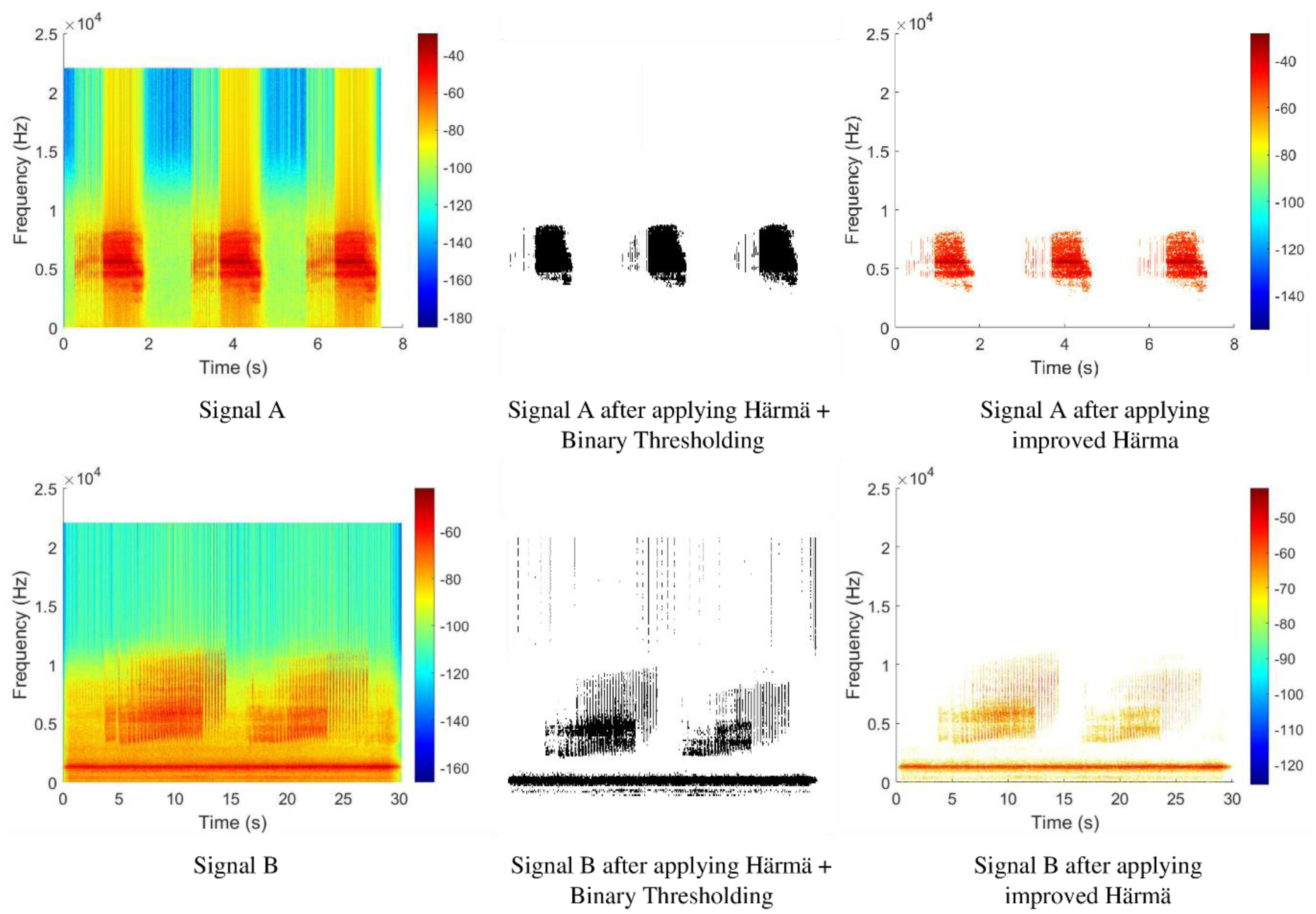
Figure 8 shows the spectrogram images of two different signals, Signal A and Signal B, before and after applying the Härmä algorithm and binary thresholding. By comparing the spectrograms of Signal A before and after processing, it was shown that most of the unnecessary information was successfully removed after applying the thresholding technique. However, the straight line appearing at the center of the binarized spectrogram that represents very low-amplitude signals was not removed due to its original blue color, which is above the threshold value.

Figure 8. Spectrogram of signals before and after segmentation.

In the case of Signal A, the result was still acceptable since the signal only has some background noises with very low amplitude, and thus, the effect of the very low-amplitude background noises was not obvious. However, if observed from the binarized spectrogram of Signal B that contains a lot of background noises with very low amplitude, the output appeared to be very noisy after applying binary thresholding.

3.5.3. Improved Härmä Syllable Segmentation

Binary thresholding has successfully removed background noises with some minor limitations. This can be further improved to produce cleaner output. In this paper, an attempt was made to remove low-amplitude background noises. Similar to the original Härmä algorithm, the improved Härmä algorithm will check if the maximum signal peak of the current time, |S(f,t)|, is greater than or equal to minAmp. From here, the algorithm was modified to check if other values at that time are above the threshold cut-off (4). The signal will be removed if its value is found to be lower than the threshold,

$$\left|S\left(\left[f_0, f_0+1, \dots , f_e\right], t\right)\right|\ge cutoff$$

(4)

where $f_0$ and $f_e$ represent the first and last row of the spectrogram matrix.

After this step, the algorithm worked the same as the original Härmä algorithm. Figure 9 shows the flowchart of the improved Härmä algorithm, where the yellow box shows the changes made. The output from the improved Härmä algorithm was plotted as a spectrogram, as shown in Figure 8. As compared to the output from the original Härmä algorithm and the output after applying the original Härmä algorithm and binary thresholding for the same signal, the output obtained using the proposed improved Härmä algorithm appeared to be cleaner and showed only the important features of the signal.

Figure 9. Flowchart of the Härmä syllable segmentation algorithm.

3.6. Spectogram Representation

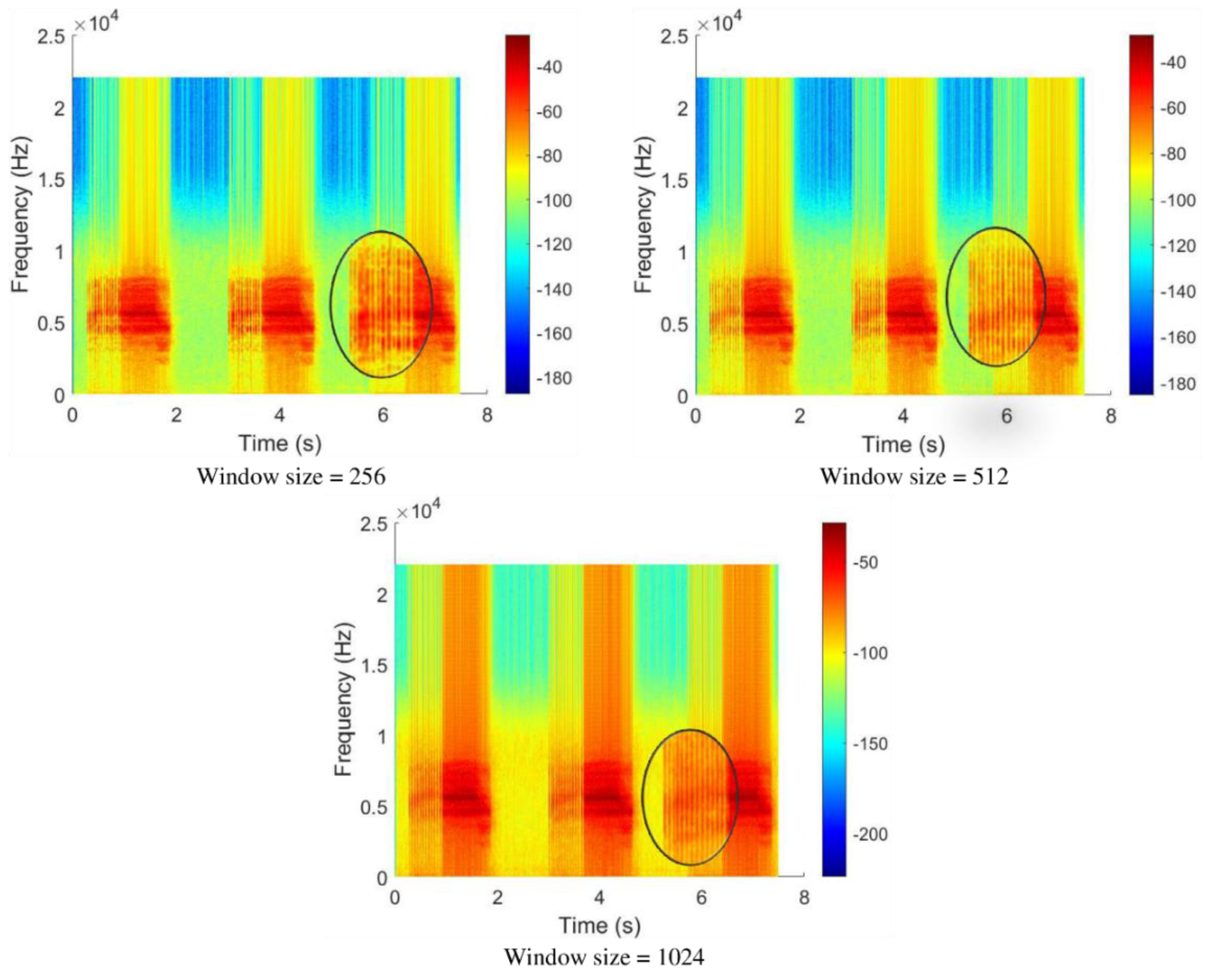
After segmenting the audio signals, the signals were transformed into spectrogram representation. The spectrogram, or time-frequency distribution plot, shows the strength of a signal over time at different frequencies by representing it with different colors [18]. In this study, different window sizes were applied to generate different spectrogram images to find which window size best suits the cicada species’ audio signals.

Initially, the window size of the spectrogram image was set to 256 points with Kaiser window, 30% overlap, and FFT size of 256 points. Figure 10 shows the resulting spectrogram image. The spectrogram successfully captured the long syllables in the signal, but the short syllables appeared to be choppy and blurry.

Figure 10. Spectrograms generated with different window sizes.

Thus, the window size was increased to 512 points and 1024 points to capture the short syllables in the signal. The spectrograms generated using the two window sizes were able to capture a clearer and more complete short syllable as compared to the spectrogram image generated using a window size of 256 points. However, if observed carefully, when using a window size of 1024 points, more background noises were captured than the other window sizes.

A trade-off was needed between the clarity of short syllables and low background noises. Therefore, a window size of 512 points was selected. In short, the spectrogram images used in this research were generated using the Kaiser window with a size of 512 points, FFT size of 256 points, and 30% overlap.

3.7. Classification with Convolutional Neural Network (CNN)

3.7.1. Input

The spectrogram representations were used as the input to a convolutional neural network (CNN) model to perform classification. Spectrograms generated using the different methods were tested, which include the spectrograms produced after applying: (1) the original Härmä algorithm, (2) the original Härmä algorithm with binary thresholding, and (3) the improved version of the Härmä algorithm.

For each version of the spectrogram images, the spectrograms were either generated from the full-length audio file or the individual syllables found from the Härmä algorithm. The spectrogram images of full-length audio formed the Full-Length Dataset used in the experiments, while the spectrogram images of individual syllables formed the Cut Dataset in the experiments. One of the reasons the Cut Dataset was created was to tackle the problem of the small dataset present in this research. By splitting the audio recordings into smaller samples based on the syllables, more samples can be obtained for each species and used for model training.

3.7.2. CNN Model

In this research, CNN was selected as the model to perform classification. CNN is a deep learning algorithm commonly used in image processing. A CNN model typically consists of a series of convolutional layers for feature mapping, pooling layers for downsampling, a fully-connected layer to flatten the input, and an output layer for prediction [19]. In the case of overfitting, dropout layers may be added to the model to randomly drop some values during training.

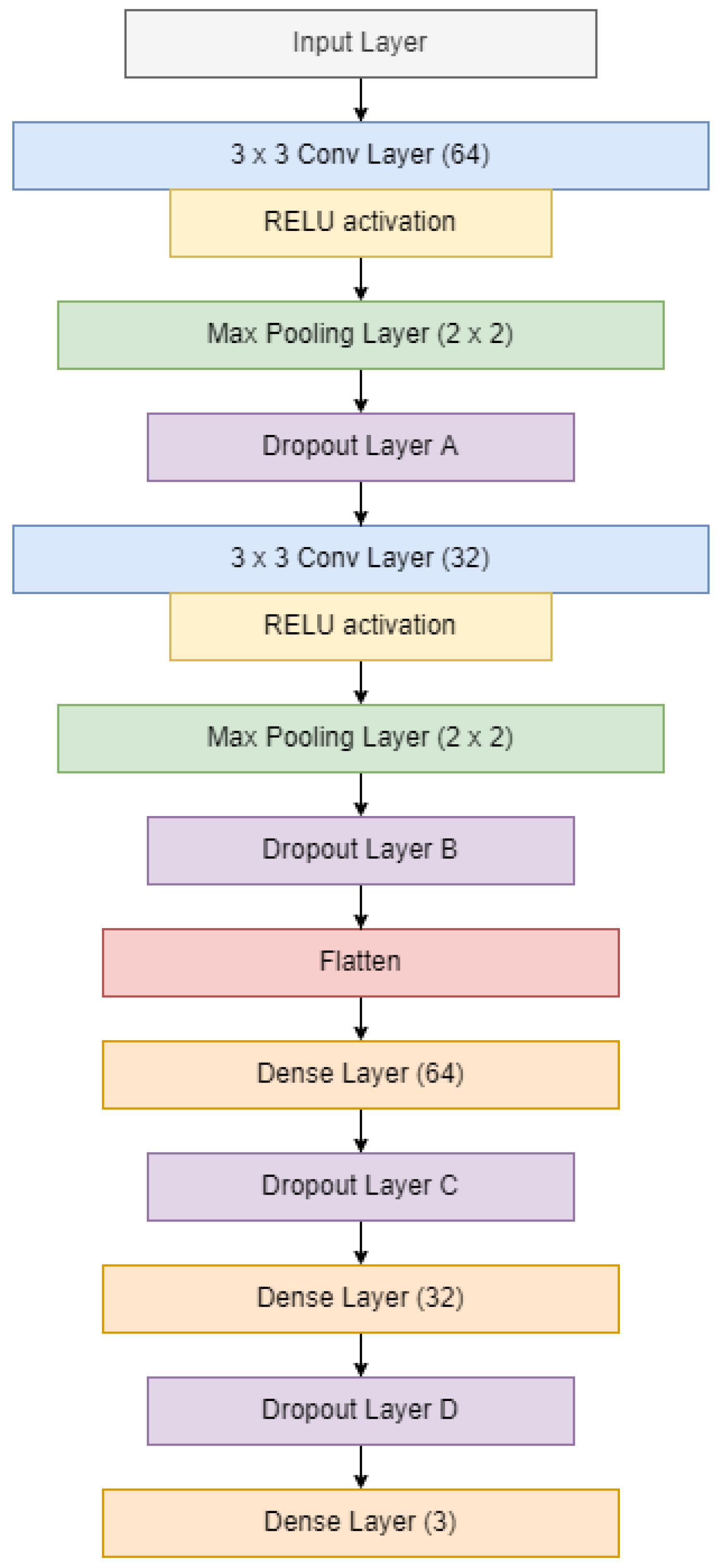
Since the dataset for this research was small, a simple CNN model was built to classify the audio signals of the three cicada species. The first layer was the input layer, which takes in spectrogram images with dimensions h × w × r, where h, w, and r represent the height and width of the image, and the number of channels, respectively. The input was passed to two sets of convolutional layers, max-pooling layers and dropout layers. Then, the output was passed to the fully-connected layer and then flattened into a one-dimensional array. The array was passed to the dense layers with 64 and 32 filters, each followed by a dropout layer. Lastly, the output layer with the Softmax activation function was used to predict the class of the input sample. Figure 11 shows the architecture of the CNN model.

Figure 11. Architecture of the CNN Model.

4. Results

Several experiments were conducted using different variations of the dataset, including the dataset after applying Härmä syllable segmentation (Härmä), Härmä with binary thresholding, and the improved version of Härmä, on both the Full-Length Dataset and the Cut Dataset.

The settings for constructing the convolutional neural network (CNN) architecture in all experiments were based on the architecture in Figure 10. All values of the dropout layers were set to 0.2. The models in the experiments were trained with 40 epochs, a batch size of 8, and by using an Adam optimizer. The model classified the species into one of the three classes, species 1 to 3, where species 1 represented Magicicada cassinii, species 2 represented Magicicada septendecim and species 3 represented Magicicada septendecula.

4.1. Benchmark Test

A preliminary test was conducted to obtain a benchmark result. The test was conducted by denoising the audio signals using a Butterworth filter and representing the signals as spectrogram images. The dataset was split with a ratio of 8:2 into training and testing datasets. The CNN model was trained with 30 epochs and a batch size of 8 and by using stochastic gradient descent (SGD) as the optimizer. The best result obtained using this setting was 77.78%.

4.2. Härmä Algorithm

In this experiment, the performance of the original Härmä algorithm was evaluated. Similar to the previous experiment, the audio signals were first denoised using the Butterworth filter. After that, the Härmä algorithm was applied. The CNN model was used to classify the spectrogram representations obtained from the Härmä algorithm. The experiments were conducted on both the Full-Length Dataset and the Cut Dataset.

4.2.1. Full-Length Dataset

The Full-Length Dataset contained the spectrogram images of size 400 × 100 pixels, generated from the complete, full-length audio recordings. The Full-Length Dataset contained 43 samples, where species 1 and 3 have 14 samples each, and species 2 has 15 samples. The dataset was split with a ratio of 8:2 into the training and testing datasets.

Based on the results presented in Table 2, the overall accuracy achieved was 66.67%. All samples of species 2 were classified correctly, but only one sample of species 1 and two samples of species 3 were predicted accurately. The result of this experiment was also lower than the result of the preliminary test. Moreover, the graphs of training and validation accuracy and loss showed signs of overfitting.

Table 2. Experimental results using the Härmä Algorithm.

Dataset	Setting	CNN Model Configuration	Accuracy
Full-Length Dataset	Butterworth filter + Härmä Algorithm+ Spectrogram + CNN	All dropout layers set to 0.2; Batch size of 8; Adam optimizer	66.67%
		First and third dropout layers set to 0.4 and 0.2 for the others; Batch size of 8; Adam optimizer	77.78%
Cut Dataset	Butterworth filter + Härmä algorithm + Spectrogram + CNN	All dropout layers set to 0.2; Batch size of 8; Adam optimizer	89.05%
		First dropout layer set to 0.4 and 0.2 for the others; Batch size of 8; Adam optimizer	92.70%

Using the same dataset, another attempt was made by modifying the architecture of the CNN model. This time, the value of the first and third dropout layers were changed to 0.4, while others remained at 0.2. The accuracy of the classification improved to 77.78% as the model has successfully classified all samples of species 2 and species 3 correctly.

4.2.2. Cut Dataset

After applying the Härmä algorithm, the individual syllables could be extracted from the audio. Thus, the Cut Dataset contained spectrogram images produced from individual syllables found in each audio. The Härmä algorithm Cut Dataset contained a total of 684 samples, with species 1 having 300 samples, species 2 having 184 samples, and species 3 having 200 samples. Similarly, the dataset was split with a ratio of 8:2 into the training and testing datasets, which made 547 samples in the training dataset and 137 samples in the testing dataset.

Using the initial settings, the model was trained using the Cut Dataset. The model achieved a high accuracy of 89.05% in classifying the three cicada species. However, the graphs of training and validation accuracy and loss showed signs of overfitting, which meant that there was still room for improvement.

Therefore, using the same dataset, the CNN model was modified by increasing the value of the first dropout layer to 0.4. The classification accuracy improved further to 92.70% after the modification. It was observed that the model was able to classify more samples of species 3 (38 out of 40) compared to the previous experiment (29 out of 40).

4.3. Härmä Algorithm and Thresholding

Next, tests were conducted using the original Härmä algorithm and binary thresholding. The CNN model was trained using the Full-Length Dataset and the Cut Dataset.

4.3.1. Full-Length Dataset

Using the initial settings where the dropout layers were set to 0.2 and a batch size of 8 with an Adam optimizer, the model was trained with the Full-Length Dataset that contained 43 samples. The model obtained an accuracy of 77.78% by classifying all samples of species 2 and 3 correctly (refer to Table 3). However, it was only able to predict one sample of species 1 correctly. Serious overfitting was also observed from the training and validation loss graphs.

Table 3. Experimental results using the Härmä algorithm and thresholding.

Dataset	Setting	CNN Model Configuration	Accuracy
Full-Length Dataset	Butterworth filter + Härmä algorithm + Thresholding + Spectrogram + CNN	All dropout layers set to 0.2; Batch size of 8; Adam optimizer	77.78%
		First and third dropout layers set to 0.4 and 0.2 for the others; Batch size of 8; Adam optimizer	77.78%
Cut Dataset	Butterworth filter + Härmä algorithm + Thresholding + Spectrogram + CNN	All dropout layers set to 0.2; Batch size of 8; Adam optimizer	88.32%
		First dropout layer set to 0.4 and 0.2 for the others; Batch size of 8; Adam optimizer	91.97%

To improve on this situation, the first and third dropout layers were modified to 0.4. The classification accuracy remained the same after the modification, but the overfitting has reduced significantly.

4.3.2. Cut Dataset

The experiment was repeated using the Cut Dataset. Since this dataset was generated by applying the original Härmä algorithm and binary thresholding, the number of samples in this dataset was the same as the dataset that applied the original Härmä algorithm only, which is 684 samples.

The initial settings of the CNN model (all dropout layers set to 0.2, batch size of 8, Adam optimizer) were used for the training process. At the end of the experiment, the model achieved a high accuracy of 88.32%. The results of this experiment were promising, but again, the graphs of training and validation loss depicted serious overfitting of the model.

To improve on the overfitting, the values of the first and third dropout layers in the CNN architecture were increased to 0.4. After the modifications, the model successfully classified all samples of species 2 correctly and was able to classify more samples of species 3 correctly (35 out of 40) compared to the previous experiment (30 out of 40).

4.4. Improved Härmä Algorithm

Experiments were also conducted to assess the performance of the improved Härmä algorithm. Similarly, the CNN model was trained using the Full-Length Dataset and the Cut Dataset.

4.4.1. Full-Length Dataset

The Full-Length Dataset used in this experiment contained the same number of samples as the Full-Length Dataset used in previous experiments. Again, the CNN model was built using the initial settings (all dropout layers set to 0.2, batch size of 8, Adam optimizer) and trained with the Full-Length Dataset. The classification accuracy obtained was higher than the accuracy achieved in the previous experiments that used Full-Length Dataset, which is 88.89% (refer to Table 4). The model has successfully identified all samples of species 2 and 3 correctly and classified two samples of species 1 accurately. Despite the high accuracy, the graphs showed that the model is seriously overfitted.

Table 4. Experimental results using the improved Härmä algorithm.

Dataset	Setting	CNN Model Configuration	Accuracy
Full-Length Dataset	Butterworth filter + Improved Härmä algorithm + Spectrogram + CNN	All dropout layers set to 0.2; Batch size of 8; Adam optimizer	88.89%
		First dropout layer set to 0.4 and 0.2 for the others; Batch size of 8; Adam optimizer	100.00%
Cut Dataset	Butterworth filter + Improved Härmä algorithm + Spectrogram + CNN	All dropout layers set to 0.2; Batch size of 8; Adam optimizer	93.02%

To further improve the model and the classification accuracy, the first dropout layer in the CNN model was changed to 0.4 and trained again with the same dataset. The results showed that the overfitting has reduced. With the improvements, the model has successfully classified all species correctly and achieved a perfect classification accuracy of 100%.

4.4.2. Cut Dataset

After applying the improved Härmä algorithm, spectrogram images were directly generated from the syllables found in each audio file, forming the Cut Dataset. The improved Härmä algorithm Cut Dataset consisted of a total of 215 samples, with 147 samples of species 1, 25 samples of species 2, and 43 samples of species 3. The dataset was split with a ratio of 8:2 into 172 training samples and 43 testing samples.

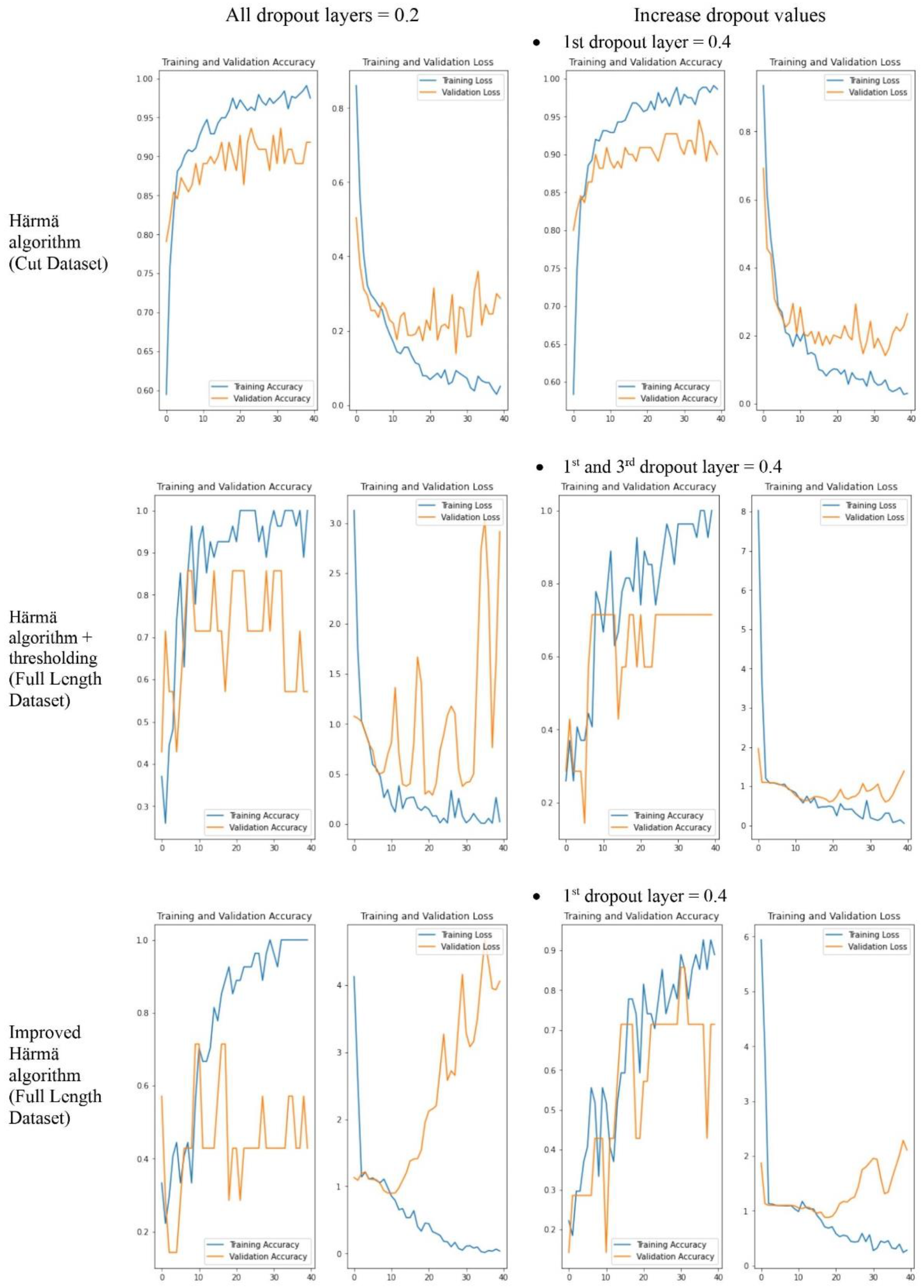
Using the initial settings to build the CNN model, the model was trained with the Cut Dataset, and the model achieved the highest accuracy compared to all the previous experiments that used the Cut Dataset, which is 93.02%. The model has successfully classified almost all samples of the three species correctly, with only one sample of each species being misclassified.

Figure 12 shows some samples of the training and validation accuracy graph and training and validation loss graph used to monitor if there is overfitting of the model. Comparisons were made between different settings, i.e., when the value of all dropout layers was set to 0.2 and when some values of the dropout layers were increased, and we were able to observe that the overfitting of the model reduced after the modification.

Figure 12. Samples of Training and Validation Accuracy and Loss Graph.

5. Discussion

A summary to compare the results of the different approaches is presented in Table 5. Overall, all the proposed methods have successfully surpassed the preliminary benchmark test, with classification accuracies ranging from 77.78% to 100%. This shows that the implementation of the Härmä algorithm is a promising direction.

Table 5. A comparison among the methods.

Method	Description	Input	Accuracy
Benchmark Test	Butterworth filter + Spectrogram + CNN	Full-Length Dataset	77.78%
Härmä algorithm	Butterworth filter + Härmä algorithm+ Spectrogram + CNN	Full-Length Dataset	77.78%
		Cut Dataset	92.70%
Härmä algorithm + Thresholding	Butterworth filter + Härmä algorithm + Thresholding + Spectrogram + CNN	Full-Length Dataset	77.78%
		Cut Dataset	91.97%
Improved Härmä algorithm	Butterworth filter + Improved Härmä algorithm+ Spectrogram + CNN	Full-Length Dataset	100%
		Cut Dataset	93.02%

From the experiments, it is observed that when passing the dataset after applying the improved version of the Härmä algorithm as input to the CNN model, the model obtains the highest classification accuracy among the variations of the dataset, which is 93.02% when using the Cut Dataset as input, and 100% when using the Full-Length Dataset as input. This shows that the improved Härmä algorithm is feasible and suitable for the recognition of cicada species. It has successfully improved the representation of the original signal and, thus, allowed the model to classify the audio signals more accurately.

When comparing the Full-Length Dataset and the Cut Dataset, it is evident that the Cut Dataset is more suitable for all versions of the approaches as the accuracies are significantly higher than that of the Full-Length Dataset. In terms of the dataset that applied the improved the Härmä algorithm, both the Full-Length Dataset and the Cut Dataset provide a promising result. This demonstrates that the proposed improved Härmä algorithm works well with the different natures of datasets.

6. Conclusions

The proposed improved Härmä algorithm has demonstrated promising results for cicada species recognition. An appealing accuracy of up to 100% can be achieved using the proposed method. The proposed cicada species recognition system is important in automating the process of monitoring and classifying periodical cicada species to save time and effort. Although various insect detection and classification systems have been proposed in numerous papers by different researchers, researchers are constantly experimenting the topic to improve the existing solutions. The opportunity to contribute to this research topic is indeed inspiring and valuable.

For future work, with more time and resources, more audio recordings will be collected to increase the size of the cicada species audio dataset. Besides, different cicada species can be investigated so that more variations of the sound of cicada species can be captured to generalize the model and the classification results can be improved further. Since this study only uses a deep learning model for training and classification, a potential direction of research can be by using different deep learning models or machine learning models for cicada species recognition. By this, a comparison among the performances of the models can be performed to find the most suitable model for the cicada species recognition task.

References

- Noda, J.J.; Travieso-González, C.M.; Sánchez-Rodríguez, D.; Alonso-Hernández, J.B. Acoustic Classification of Singing Insects Based on MFCC/LFCC Fusion. Appl. Sci. 2019, 9, 4097. [Google Scholar] [CrossRef]
- Fuhr, P.L.; Rooke, S.S.; Morganti, M.; Grant, E.; Piersall, E.; Richards, J.; Wilson, A.; Monday, W.; King, T.J., Jr. Frequency and Temporal Analysis of Cicada Brood X Sounds. Int. Res. J. Eng. Technol. 2021, 8, 9. [Google Scholar]
- Young, D.; Josephson, R.K. Pure-tone songs in cicadas with special reference to the genusMagicicada. J. Comp. Physiol. A Sens. Neural Behav. Physiol. 1983, 152, 197–207. [Google Scholar] [CrossRef]
- Reid, K.H. Periodical Cicada: Mechanism of Sound Production. Science 1971, 172, 949–951. [Google Scholar] [CrossRef] [PubMed]
- Chauhan, N.K.; Singh, K. A Review on conventional machine learning vs. deep learning. In Proceedings of the 2018 International Conference on Computing, Power and Communication Technologies (GUCON), Greater Noida, India, 28–29 September 2018; pp. 347–352. [Google Scholar] [CrossRef]
- Subasi, A. Feature extraction and dimension reduction. In Practical Guide for Biomedical Signals Analysis Using Machine Learning Techniques; Elsevier: Amsterdam, The Netherlands, 2019; pp. 193–275. [Google Scholar] [CrossRef]
- Potamitis, I.; Ganchev, T.; Fakotakis, N. Automatic acoustic identification of crickets and cicadas. In Proceedings of the 2007, 9th International Symposium on Signal Processing a1&nd ITAS Applications, Sharjah, United Arab Emirates, 12—15 February 2007; pp. 1–4. [Google Scholar] [CrossRef]
- Leqing, Z.; Zhen, Z. Insect sound recognition based on SBC and HMM. In Proceedings of the 2010 International Conference on Intelligent Computation Technology and Automation, Changsha, China, 11—12 May 2010; pp. 544–548. [Google Scholar] [CrossRef]
- Kawakita, S.; Ichikawa, K. Automated classification of bees and hornet using acoustic analysis of their flight sounds. Apidologie 2019, 50, 71–79. [Google Scholar] [CrossRef]
- Murugaiya, R.; Abas, P.E.; De Silva, L.C. Probability Enhanced Entropy (PEE) Novel Feature for Improved Bird Sound Classification. Mach. Intell. Res. 2022, 19, 52–62. [Google Scholar] [CrossRef]
- Chesmore, D. Automated bioacoustic identification of species. An. Acad. Bras. Ciências 2004, 76, 436–440. [Google Scholar] [CrossRef] [PubMed]
- Zamanian, H.; Pourghassem, H. Insect identification based on bioacoustic signal using spectral and temporal features. In Proceedings of the 2017 Iranian Conference on Electrical Engineering (ICEE), Tehran, Iran, 2–4 May 2017; pp. 1785–1790. [Google Scholar] [CrossRef]
- Dong, X.; Yan, N.; Wei, Y. Insect sound recognition based on convolutional neural network. In Proceedings of the 2018 IEEE 3rd International Conference on Image, Vision and Computing (ICIVC), Chongqing, China, 27–29 June 2018; pp. 855–859. [Google Scholar] [CrossRef]
- Arpitha, M.S.; Rani, S.R.K.; Lavanya, M.C. CNN based framework for classification of mosquitoes based on its wingbeats. In Proceedings of the 2021, Third International Conference on Intelligent Communication Technologies and Virtual Mobile Networks (ICICV), Tirunelveli, India, 4–6 February 2021; pp. 1–5. [Google Scholar] [CrossRef]
- Zhang, M.; Yan, L.; Luo, G.; Li, G.; Liu, W.; Zhang, L. A Novel insect sound recognition algorithm based on MFCC and CNN. In Proceedings of the 2021 6th International Conference on Communication, Image and Signal Processing (CCISP), Chengdu, China, 19–21 November 2021; pp. 289–294. [Google Scholar] [CrossRef]
- Eleftheriadis, C.; Karakonstantis, G. Energy-Efficient Fast Fourier Transform for Real-Valued Applications. IEEE Trans. Circuits Syst. II Express Briefs 2022, 69, 2458–2462. [Google Scholar] [CrossRef]
- Harma, A. Automatic identification of bird species based on sinusoidal modeling of syllables. In Proceedings of the 2003 IEEE International Conference on Acoustics, Speech, and Signal Processing, Hong Kong, China, 6–10 April 2003; pp. 545–554. [Google Scholar] [CrossRef]
- Tanveer, M.H.; Zhu, H.; Ahmed, W.; Thomas, A.; Imran, B.M.; Salman, M. Melspectrogram and deep CNN based representation learning from bio-sonar implementation on UAVs. In Proceedings of the 2021 International Conference on Computer, Control and Robotics (ICCCR), Shanghai, China, 8–10 January 2021; pp. 220–224. [Google Scholar] [CrossRef]
- He, X.; Chen, Y.; Huang, L. Toward a Trustworthy Classifier with Deep CNN: Uncertainty Estimation Meets Hyperspectral Image. IEEE Trans. Geosci. Remote Sens. 2022, 60, 5529115. [Google Scholar] [CrossRef]