Article

Modifications of Flower Pollination, Teacher-Learner and Firefly Algorithms for Solving Multiextremal Optimization Problems †

by
Pavel Sorokovikov
* and
Alexander Gornov
Optimal Control Laboratory, Matrosov Institute for System Dynamics and Control Theory, Siberian Branch, Russian Academy of Sciences, 664033 Irkutsk, Russia
*
Author to whom correspondence should be addressed.
This paper is an extended version of our paper published in the proceedings of the 10th International Workshop on Mathematical Models and their Applications (IWMMA 2021) (Krasnoyarsk, Russian Federation, 16–18 November 2021).
Algorithms 2022, 15(10), 359; https://doi.org/10.3390/a15100359
Submission received: 30 August 2022 / Revised: 24 September 2022 / Accepted: 26 September 2022 / Published: 28 September 2022
(This article belongs to the Special Issue Mathematical Models and Their Applications III)

Abstract

:
The article offers a possible treatment for the numerical research of tasks which require searching for an absolute optimum. This approach is established by employing both globalized nature-inspired methods as well as local descent methods for exploration and exploitation. Three hybrid nonconvex minimization algorithms are developed and implemented. Modifications of flower pollination, teacher-learner, and firefly algorithms are used as nature-inspired methods for global searching. The modified trust region method based on the main diagonal approximation of the Hessian matrix is applied for local refinement. We have performed the numerical comparison of variants of the realized approach employing a representative collection of multimodal objective functions. The implemented nonconvex optimization methods have been used to solve the applied problems. These tasks utilize an optimization of the low-energy metal Sutton-Chen clusters potentials with a very large number of atoms and the parametric identification of the nonlinear dynamic model. The results of this research confirms the performance of the suggested algorithms.

1. Introduction

1.1. Background and Related Work

The global optimization of multimodal objective functions remains a crucial and difficult mathematical problem. Currently, much attention in the scientific literature is paid to approximate methods for global optimization [1], which allow for the possibility of finding a “high quality” solution in an acceptable (from a practical point of view) time. Among them, metaheuristic optimization methods are widely used [2]. Unlike classical optimization methods, metaheuristic methods can be used in situations where information about the nature and properties of the function under study is almost completely absent. Heuristic methods based on intuitive approaches make it possible to find sufficiently good solutions to the problem without proving the correctness of the procedures used and the optimality of the result obtained. Metaheuristic methods combine one or more heuristic methods (procedures) based on a higher-level search strategy. They are able to leave the vicinity of local extrema and perform a fairly complete study of the set of feasible solutions.
The classification of metaheuristic methods is currently conditional, since the characteristic groups of methods are based on similar ideas. For example, well-known bioinspired algorithms can be divided into the following categories:
  • Evolutionary algorithms (evolutionary strategies, genetic search, biogeography-based algorithms, differential evolution, others) [2,3,4,5,6,7,8,9,10,11,12];
  • “Wildlife-inspired” algorithms [2,13,14,15,16,17,18,19,20,21];
  • Algorithms inspired by human community or inanimate nature [2,13,22,23,24,25,26]; etc.
The Flower Pollination (FP) algorithm was proposed by X.S. Yang in 2012 at the University of Cambridge (UK) (see, for example, [9,14]). The Teaching-Learning-based optimization (TL) algorithm was proposed by R. Rao in 2011 (see, e.g., [9,22,23]).
The swarm optimization method, which mimics the behavior of fireflies, borrows ideas from observing fireflies that engage with partners, attracting them with their light. Agents (fireflies) forming a swarm use dynamic decision sets to choose neighbors and find the direction of movement, which is determined by the strength of the signal emanating from them. X.S. Yang from the University of Cambridge proposed the firefly algorithm (FA) in 2007 (see, for instance, [15,16,17,18]). For example, the known modifications of the method are the Gaussian FA [17], chaotic FA [18], and others.
Recent molecular physics methods resolve to obtain a meaningful understanding of the structure of different substances [27]. Searching for atomic-molecular clusters with a low potential is one of the classical problems of computational chemistry (see, for example, [28]). This problem is reduced to finding the minimum of potential functions in the form of special mathematical models that have already been created for several hundreds of structures. The Cambridge Energy Landscape Database [29] presents the results of global optimization for various types of models: inert gas clusters, metal clusters, ionic clusters, silicon and germanium clusters, and others. The main difficulty with problems in this class is their non-convexity, which is expressed by a huge number of local extremes of potential functions. Experts give estimates that, in some cases, prove an exponential increase in the number of local extrema from the number of atoms or optimized variables. The most famous and frequently considered potential functions in the scientific literature are the models of Lennard-Jones, Morse, Keating, Gupta, Dzugutov, Sutton-Chen and others. Since the exact value of the global minimum is unknown in most cases, the principle of presenting the “best of known” solutions are used in the works of this direction. This means that the presented solution is “probably optimal”, until one of the experts finds a lower value.
Regular studies regarding optimization problems formulated for the potentials of atomic-molecular clusters began in the 1990s by specialists from Great Britain and the USA [28]. At this stage, for the Sutton-Chen potential, for example, only 80 atoms were recorded as indicators of the dimension of the problems, which corresponds to 240 variables for the optimized function, but the number of local extrema in the recorded problems were already estimated by an astronomical indicator − 10 60 . The search for a solution to optimize problems for low-potential clusters of ever-increasing dimensions continues to be an urgent problem, due to the emergence of similar formulations in chemistry, physics, materials science, nanoelectronics, nanobiology, pharmaceuticals, and other fields [30].

1.2. Question and Contributions

The article suggests an approach that applies the advantages of nature-inspired algorithms for the global exploration and first order methods for local optimization. We applied modifications of the following bioinspired methods for global search: flower pollination, teacher-learner, and firefly algorithms. The modified trust region method [31,32] based on the main diagonal approximation of the Hessian matrix [33] is used for local minimization. The proposed approach makes it possible to create computational schemes that make it possible to efficiently solve global optimization problems. It is also necessary at each iteration of the algorithm to ensure that the population is sufficiently diverse. For this purpose, biodiversity assessment was introduced into the proposed algorithm schemes.
The article is organized in the following way: Section 1.3 formulates the statement of the non-local optimization problem; Section 2 presents the developed hybrid algorithms based on nature-inspired and local descent methods; Section 3 describes performed computational experiments on a set of test and applied optimization tasks, presents numerical study results; Section 4 concludes the paper.

1.3. The Global Optimization Problem

We consider a global optimization problem with parallelepiped constraints. The problem statement is the following:
f ( x ) min ,   x X ,   X = { x | x = ( x 1 , x 2 , , x n ) ,   α i x i β i ,   i = 1 , n ¯ } .
Here, f ( x ) is the smooth and multiextremal objective function; n N is the number of arguments (dimension); α R n ,   β R n are box constraints.

2. Description of Proposed Algorithms

Three multiextremal optimization algorithms established on flower pollination, teacher-learner, firefly, trust region methods are developed and implemented. This section introduces them.

2.1. Algorithm Based on Flower Pollination and Local Search Methods

2.1.1. Parameters

  • m [ 5 ;   10000 ] Z —number of agents;
  • N L O C [ 0 ;   10000 ] Z – number of iterations of the local search method;
  • ε b i o [ 0 ;   0.1 ] R —biodiversity factor;
  • P s [ 0 ;   1 ] R —switching probability, it puts control on global and local pollination (search) procedures.

2.1.2. Step-by-Step Algorithm

We have implemented two variants of the FP: the original one, which uses only the objective function value (v.1, N L O C = 0 ), and the modified one, in which the minimization trajectory is constructed established on the modified trust region method (v.2, N L O C > 0 ), beginning from each point obtained by using the “flower pollination” procedure. In both variants, a measure of biodiversity is calculated at the sixth step. See Algorithm 1.
Algorithm 1 FP
  • Set the algorithmic parameters. Choose starting point x 0 X . Suppose x R E C = x 0 , where x R E C is the record point. Compute f R E C = f ( x R E C ) . Suppose K = 0 , where K is the algorithm iteration number.
  • Create a random initial set of agents (population) P 0 = { p 1 = x 0 , p 2 , , p m } , p j X ,     j = 1 , m ¯ .
  • Carry out a selection of the initial population: perform m local descents, each of N L O C iterations of the local search method, each starts with its agent (individual) of the initial population, get { s 1 , s 2 , , s m } .
  • Improve the record point, take x R E C = arg min { f ( s l ) , l = 1 , m ¯ } .
  • Substitute in the population P 0 of the individuals { p 1 , p 2 , , p m } by the agents { s 1 , s 2 , , s m } .
    On the K -th iteration:
  • Calculate a measure of biodiversity M b i o = 1 / ( m 1 ) l = 1 m 1 p l + 1 p l .
  • If the stoppage criterion M b i o < ε b i o is satisfied, then output x R E C , the algorithm is terminated.
  • Build a tentative population. In a cycle for each l = 1 , m ¯ :
    8.1.
    Create a random numeric r l [ 0 , 1 ] R .
    8.2.
    If r l P s , then a vector L of size m is formed, which obeys the Levy distribution (see, for example, [13,14]); a “global pollination” is performed: p n e w = p l + L ( p l x R E C ) .
    8.3.
    If r l > P s , then generate two random indexes j 1 , j 2 :   j 1 j 2 (one of the two integer indexes j 1 , j 2 can be equal to the index l ), generate a random number ε [ 0 , 1 ] R , perform a “local pollination”: p n e w = p l + ε ( p j 1 p j 2 ) .
    8.4.
    The old agent is replaced with a new one (in case of improvement): if f ( p n e w ) f ( p l ) , then p l = p n e w .
  • Evaluate all agents: in a cycle for l = 1 , m ¯ execute N L O C iterations of the local search method, each starts with its individual in the population p l , get a multitude of agents { s 1 , s 2 , , s m } .
  • Improve the record point, take x R E C = arg min { f ( s l ) , l = 1 , m ¯ } .
  • Select m best agents from the two multitudes P K and { s 1 , s 2 , , s m } to the new set, get P K + 1 .
  • Set K = K + 1 , move to stage 6.
The iteration is complete.

2.2. Algorithm Based on Teacher-Learner and Local Descent Methods

2.2.1. Parameters

  • m [ 5 ;   10000 ] Z —number of students;
  • N L O C [ 0 ;   10000 ] Z —number of iterations of the local search method;
  • ε b i o [ 0 ;   0.1 ] R —biodiversity factor.

2.2.2. Step-by-Step Algorithm

Two variants of the TL have been implemented: the original (v.1, N L O C = 0 ) and the hybridized with the modification of trust region (v.2, N L O C > 0 ) method for local descents. See Algorithm 2.
Algorithm 2 TL
  • Set the algorithmic parameters. Choose starting point x 0 X . Suppose x R E C = x 0 , where x R E C is the record point. Compute f R E C = f ( x R E C ) . Suppose K = 0 , where K is the algorithm iteration number.
  • Create a random initial set of agents (a group of students) P 0 = { p 1 = x 0 , p 2 , , p m } , p j X ,     j = 1 , m ¯ .
  • Carry out a selection of the initial population: perform m local descents, each of N L O C iterations of the local search method, each starts with its agent (student) of the initial population, get { s 1 , s 2 , , s m } .
  • Improve the record point, take x R E C = arg min { f ( s l ) , l = 1 , m ¯ } .
  • Substitute in the group P 0 of the students { p 1 , p 2 , , p m } by the agents { s 1 , s 2 , , s m } .
    On the K -th iteration:
  • Calculate a measure of biodiversity M b i o = 1 / ( m 1 ) l = 1 m 1 p l + 1 p l .
  • If the stoppage criterion M b i o < ε b i o is satisfied, then output x R E C , the algorithm is terminated.
  • Teacher stage:
    8.1.
    The average value of the objective function of the entire group M e a n = 1 / m · ( f ( p 1 ) + + f ( p m ) ) is calculated.
    8.2.
    The best agent (teacher) p t e a c h is found.
    8.3.
    In a cycle for each l = 1 , m ¯ : create random numbers r 1 , r 2 [ 0 ,   1 ] R ; T F = r o u n d ( 1 + r 2 ) ; p n e w = p l + r 1 ( p t e a c h T F · M e a n ) .
    8.4.
    If the new solution is better than the existing one, then the resulting solution is accepted, otherwise the existing solution is kept (if f ( p n e w ) f ( p l ) , then p l = p n e w ).
  • Learner stage:
    9.1.
    In a cycle for each l = 1 , m ¯ : create two random indexes j 1 , j 2 :   j 1 j 2 , a random numeric r [ 0 , 1 ] R .
    9.2.
    If f ( p j 1 ) f ( p j 2 ) , then p n e w = p l + r ( p j 1 p j 2 ) , else p n e w = p l + r ( p j 2 p j 1 ) .
    9.3.
    If the new solution is better than the existing one, then the resulting solution is accepted, otherwise the existing solution is kept (if f ( p n e w ) f ( p l ) , then p l = p n e w ).
  • Evaluate all students: in a cycle for l = 1 , m ¯ execute N L O C iterations of the local search method, each starts with its own agent p l , get { s 1 , s 2 , , s m } .
  • Improve the record point, take x R E C = arg min { f ( s l ) , l = 1 , m ¯ } .
  • Select m best students from the two multitudes P K and { s 1 , s 2 , , s m } to the new group, get P K + 1 .
  • Set K = K + 1 , move to stage 6.
The iteration is complete.

2.3. Algorithm Based on Firefly and Local Search Methods

2.3.1. Parameters

  • m [ 5 ;   10000 ] Z —number of fireflies;
  • N L O C [ 0 ;   10000 ] Z —number of iterations of the local search method;
  • ε b i o [ 0 ;   0.1 ] R —biodiversity factor;
  • α ˜ [ 0 ;   1 ] R —mutation coefficient;
  • β ^ 0 [ 0 ;   3 ] R —attraction ratio;
  • γ [ 0 ;   1 ] R —light absorption factor;
  • M [ 0.1 ;   10 ] R —power rate.

2.3.2. Step-by-Step Algorithm

We have implemented two variants of the FA: the classic version (v.1, N L O C = 0 ) and the combined with the modified trust region (v.2, N L O C > 0 ) method for local search. In the proposed algorithm, the biodiversity coefficient is used, which makes it possible to evaluate the measure of biodiversity and, if necessary, increase the representativeness of the training set in order to increase the final efficiency of the algorithm. See Algorithm 3.
Algorithm 3 FA
  • Perform the first five steps of Algorithm 1. The set of agents is called a population of fireflies, one agent is called a firefly (individual).
    On the K -th iteration:
  • Calculate a measure of biodiversity M b i o = 1 / ( m 1 ) l = 1 m 1 p l + 1 p l .
  • If the stoppage criterion M b i o < ε b i o is satisfied, then output x R E C , the algorithm is terminated.
  • Produce a new population Q K = { q 1 , q 2 , , q m } , f ( q i ) = ,     i = 1 , m ¯ .
  • Change a population Q K . In a cycle for each l = 1 , m ¯ and j = 1 , m ¯ : if f ( p j ) < f ( p l ) , then
    5.1.
    Compute the prettiness of the firefly p l to the individual p j : β ^ 1 = β ^ 0 · exp ( γ d l j M ) , where d l j is Euclidean distance between the fireflies p l and p j .
    5.2.
    Create a random numeric r l j [ 1 , 1 ] R .
    5.3.
    The individual p l moves towards the firefly p j . Create a new individual p n e w = p l + β ^ 1 ( p j p l ) + α ˜ · δ · r l j , where δ = 0.05 · β α .
    5.4.
    If f ( p n e w ) < f ( q i ) , then q i = p n e w .
  • Calculate a biodiversity measure M ˜ b i o = 1 / ( m 1 ) l = 1 m 1 q l + 1 q l .
  • If M ˜ b i o < ε b i o , then go to step 5, else go to step 8.
  • Evaluate all fireflies: in a cycle for l = 1 , m ¯ execute N L O C iterations of the local search method, each starts with its own firefly q l , get { s 1 , s 2 , , s m } .
  • Improve the record point, take x R E C = arg min { f ( s l ) , l = 1 , m ¯ } .
  • Select m best fireflies from the two multitudes P K and { s 1 , s 2 , , s m } to the new population, form P K + 1 . Set K = K + 1 , move to stage 2.
The iteration is complete.

3. Numerical Study of Developed Algorithms

The algorithms were implemented in C (GCC/MinGW) using uniform software standards and studied on a set of test problems [34,35]. Table 1 contains the values of algorithmic parameters. A numerical study of the properties of the proposed algorithms is carried out in comparison with other algorithms presented by us earlier in the [36]: modifications of genetic (GA), biogeography (BBO) and particle swarm (PSO) algorithms.
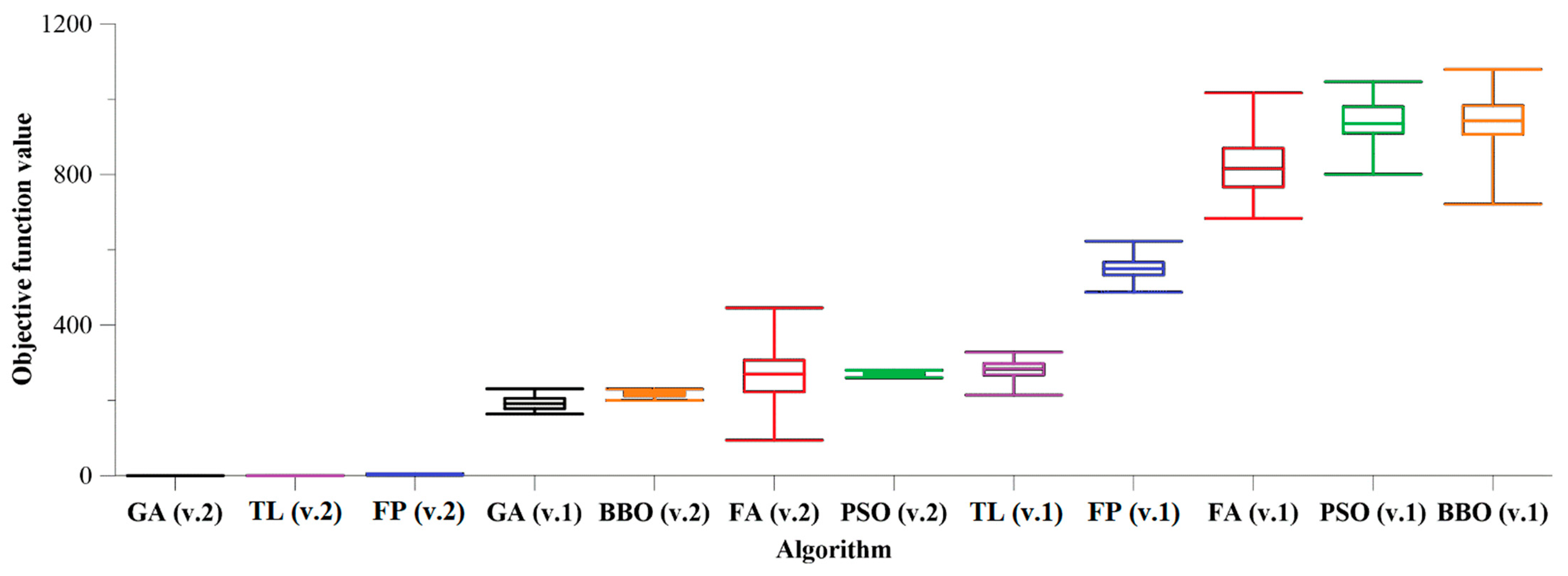
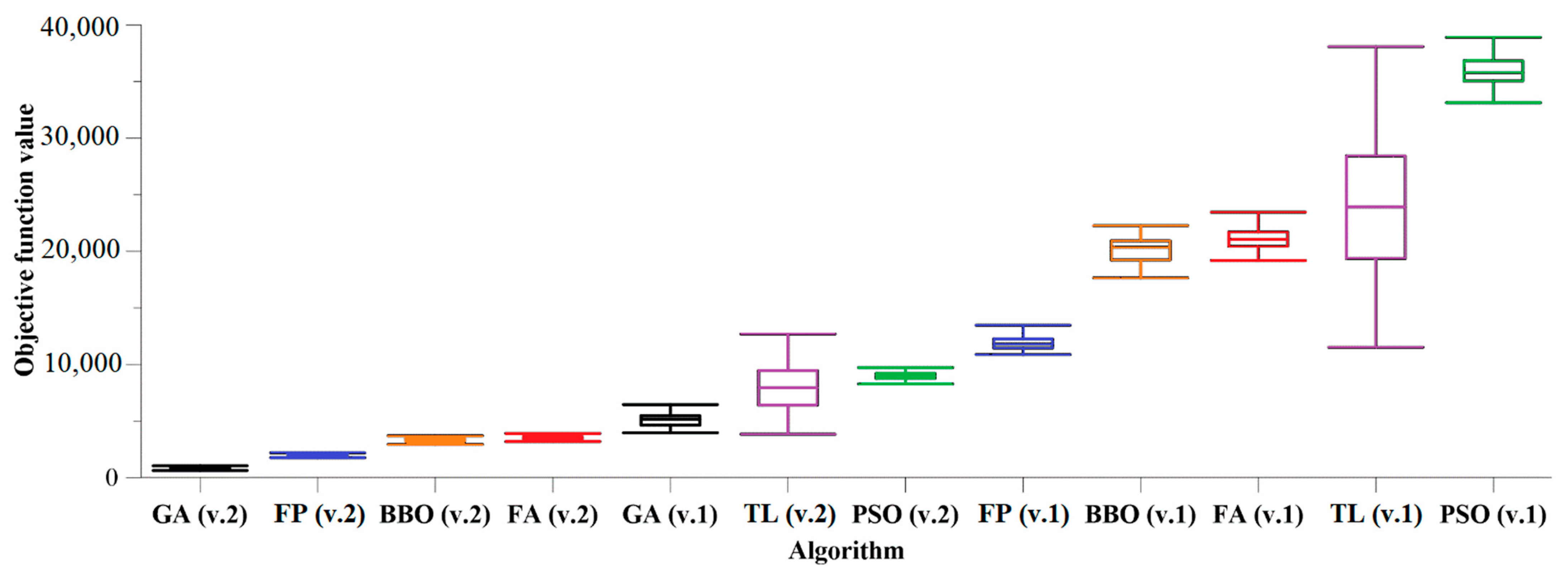
The equal testing requirements were assured for every algorithm. The number of agents for all algorithms is m = 10 . The number of task variables is 100. We launched the algorithms 50 times from the same uniformly distributed initial approximations. The additional stop criterion is exceeding 10,000 calls to the objective function. Below is an exposition of each optimization task and the results of numerical comparison of algorithms in the form of box diagrams for this test problem (Figure 1, Figure 2, Figure 3 and Figure 4). The ordinate axle plots the mean values of the objective function over the set of agents, received from 50 launches. Table 2 shows statistics on algorithmic launches.
We conducted numerical experiments applying a computer with the following characteristics: 2x Intel Xeon E5-2680 v2 2.8 GHz (20 cores); 128 Gb DDR3 1866 MHz.

3.1. The Griewank Problem

f ( x ) = 1 + i = 1 n ( x i 2 4000 ) i = 1 n cos ( x i i ) ,   X = [ 600.0 ,   600.0 ] n ,   n = 100 .
Absolute minimum point and value: x i * = 0.0 ,   f * = 0.0 .
Figure 1 and Table 2 show that the developed modifications (v.2) demonstrated essentially better results in comparison to basic variants of algorithms (v.1). On this problem, the TL algorithm turned out to be the most effective among the proposed algorithms.

3.2. The Rastrigin Problem

f ( x ) = 10 · n + i = 1 n ( x i 2 10 · cos ( 2 π x i ) ) ,   X = [ 5.12 ,   5.12 ] n ,   n = 100 .
Absolute minimum point and value: x i * = 0.0 ,   f * = 0.0 .
TL (v.2), GA (v.2), and FP (v.2) are leading amid the algorithms investigated, giving solutions close to the absolute minimum (Figure 2, Table 2).

3.3. The Schwefel Problem

f ( x ) = 418.9829 · n + i = 1 n ( x i · sin ( | x i | ) ,   X = [ 500.0 ,   500.0 ] n ,   n = 100 .
Absolute minimum point and value: x i * = 420.9687 ,   f * = 0.0 .
On the Schwefel problem, the modified algorithms (v.2) showed preferably results in comparison to basic versions (v.1) of algorithms (see Figure 3, Table 2).

3.4. The Ackley Problem

f ( x ) = 20 · e 0.2 · 1 n · i = 1 n x i 2 e 1 n · i = 1 n cos ( 2 π x i ) + 20 + e ,   X = [ 30.0 ,   30.0 ] n ,   n = 100 .
Absolute minimum point and value: x i * = 0.0 ,   f * = 0.0 .
GA (v.2) and TL (v.2) well benefits in productivity compared to otherwise developed algorithms on this problem (Figure 4 and Table 2).

3.5. The Sutton-Chen Problem

We consider finding the low-energy Sutton-Chen clusters task [37,38,39,40] for extremely large dimensions. The Sutton-Chen potential is often used in computations of the nanocluster properties of metals such as silver, rhodium, nickel, copper, gold, platinum, and others [38,39,40]. The following global optimization problem is considered:
f ( x ) = ε i [ 1 2 j i ( a r i j ) q c j i ( a r i j ) m ] min , r i j = ( x 3 ( i 1 ) + 1 x 3 ( j 1 ) + 1 ) 2 + ( x 3 ( i 1 ) + 2 x 3 ( j 1 ) + 2 ) 2 + ( x 3 ( i 1 ) + 3 x 3 ( j 1 ) + 3 ) 2 .
Here, ε = 1.0 ,   c = 144.41 ,   a = 1.0 ,   q = 12.0 ,   m = 6.0 are special parameters.
To investigate the problems of the optimization of atomic-molecular cluster potentials, we implemented three-phase computational technology, which combines several methods from a collection of basic at each phase [41].
Phase 1 is concentrated on the random approximation of a neighborhood of a record point and established on a collection of algorithms that generates starting approximations: “level” (LG), “averaged” (AG), “gradient” (GG), “level-averaged” (LAG), “level-gradient” (LGG), “averaged-gradient” (AGG), “level-averaged-gradient” (LAGG). At the phase 2, the problem of descent of the approximations produced at the phase 1 [42] is determined by applying one of the “starter algorithms” that can find low-energy configurations of atoms. We implemented six variants of “starter algorithms”: three bioinspired algorithms described in the paper (FP, TL, FA), the variant of the method proposed by B.T. Polyak [43,44], the “raider method” [45], and the modification of the multivariate dichotomy method [46,47]. In all these algorithms we applied the modification of trust region method for local search (phase 3).
Nowadays, solutions are presented only for Sutton-Chen configurations up to 80 atoms in the Cambridge Energy Landscape Database [29] and other public sources. We made a performance investigation of developed techniques for clusters of 3–80 atoms and compared the solutions obtained with the best of the known ones [48]. The solutions obtained during numerical study coincided with the known results represented in [29].
We investigated very large problems for configurations of atoms from 81 to 100. For each algorithm-generator and each starter method, we performed computational experiments. We used an excess of the time limit (24 h) as a stopping criterion. Table 3 presents the results of the numerical testing of computational technology for the task in which the cluster consists of 85 atoms.
As can be noticed from Table 3, there is a leading computational technology with a combination of the LAGG as an initial approximation generator and the raider algorithm as a starter, among all the investigated variants.
Table 4 presents the best-found values obtained. It was not possible to compare our results with the computations of other researchers due to the absence of such information.
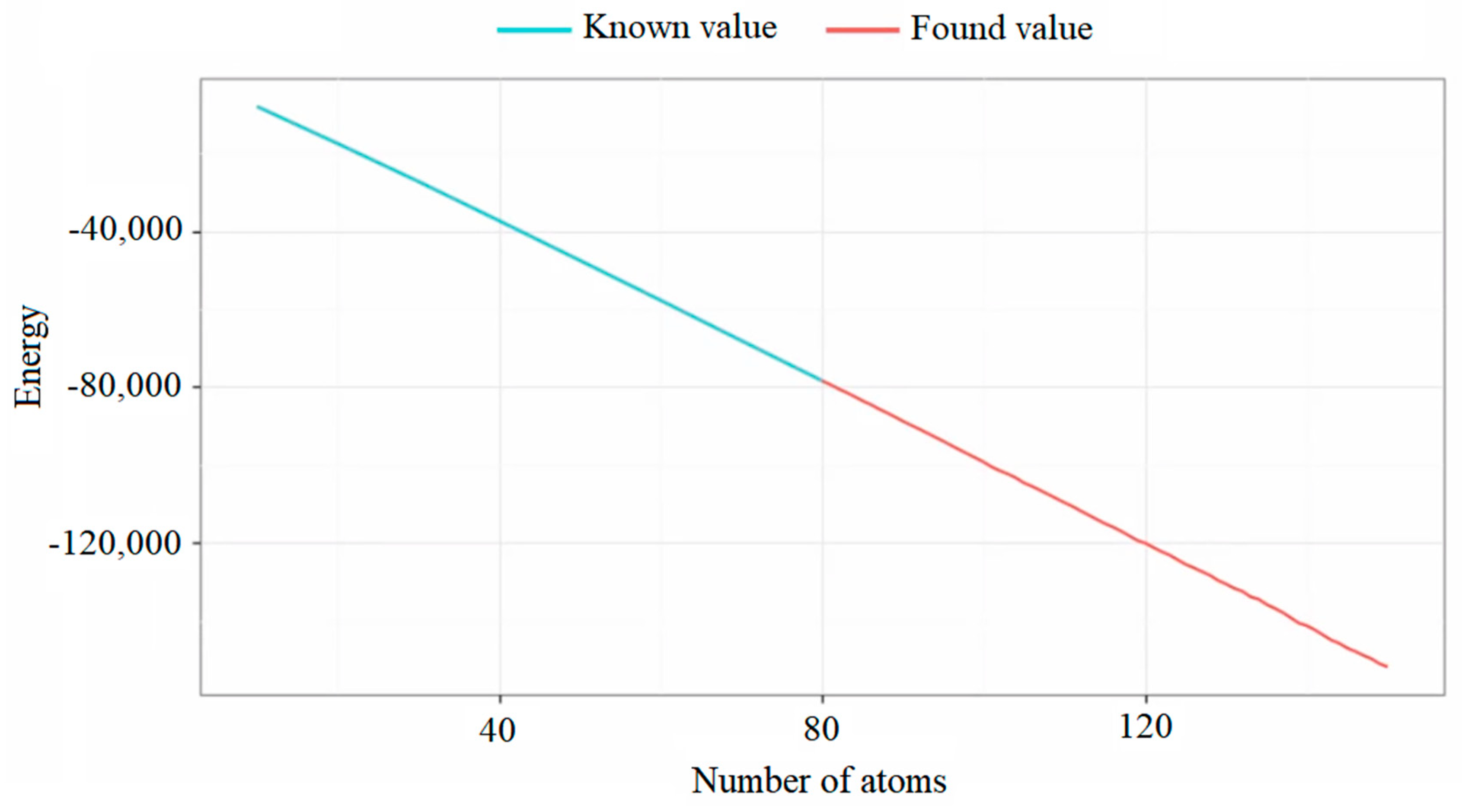
Figure 5 demonstrates the dependency of the best-found values on the dimension. We plot the number of atoms along the horizontal axis, the found values along the vertical.

3.6. The Parametric Identification Problem for the Nonlinear Dynamic Model

The proposed algorithms are universal and allow one to investigate problems of a wide class. For example, those that go beyond the considered finite-dimensional setting are dynamic problems. The tasks of parametric identification are to find the values of the model parameters that make it possible to ensure its closeness to the experimental data.
Table 5 presents the known data corresponding to the dynamics of the changes in the trajectories x ¯ ( t ) ,   y ¯ ( t ) ,   z ¯ ( t ) over time t [ 0 ,   8 ] .
With the help of the proposed algorithms, the model problem of the parametric identification of the following dynamic system was solved:
{ x ˙ ( t ) = b 1 A 1 x ( t ) + a 12 x ( t ) y ( t ) + a 13 x ( t ) z ( t ) , y ˙ ( t ) = b 2 A 2 y ( t ) a 21 x ( t ) y ( t ) + a 23 y ( t ) z ( t ) , z ˙ ( t ) = b 3 A 3 z ( t ) a 31 x ( t ) z ( t ) a 32 y ( t ) z ( t ) .
As the functional to be optimized, we used the integral of the modular discrepancy of the system (7) values x ( t ) ,   y ( t ) ,   z ( t ) and known values x ¯ ( t ) ,   y ¯ ( t ) ,   z ¯ ( t ) (see Table 5) in the time span t [ 0 ,   8 ] :
0 8 ( | x ( t ) x ¯ ( t ) | + | y ( t ) y ¯ ( t ) | + | z ( t ) z ¯ ( t ) | ) d t   min .
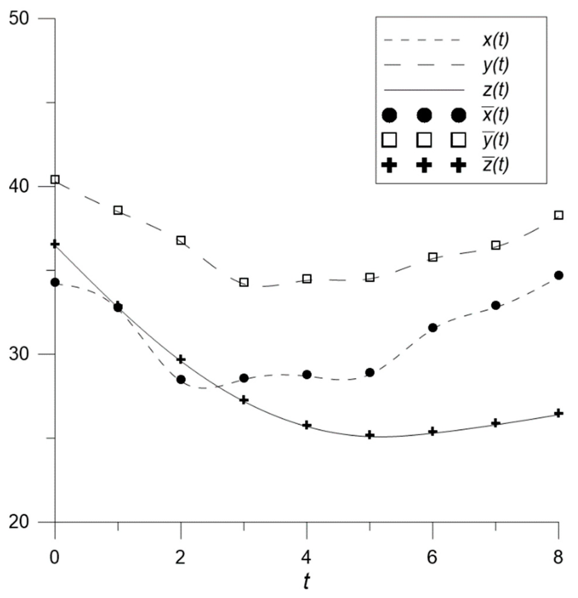
Figure 6 demonstrates the trajectories received in solving the model parametric identification problem, relative to the tabular data presented in Table 5. Time t is plotted on the graph along the abscissa.
As can be seen from the Figure 6, with the help of the proposed algorithms, it was possible to ensure the closeness of the model (7) to the experimental data (Table 5), which indicates the good performance of the algorithms.

3.7. Statistical Testing of Proposed Algorithms

We tested the implemented algorithms on the optimization benchmark [34]. As test problems, we selected 22 multimodal objective functions (numbered 7 to 28 in the benchmark). The dimensions of all problems were 100 variables. We compared the algorithms with each other and ranked them for each task. For each algorithm, we calculated the percentage of the number of problems on which it showed a certain place in the rating. Table 6 shows the results of statistical testing of combined algorithms in the following format: “percentage of reaching a certain place in the rating (the number of tasks on which this was achieved)”.
Established on the performed computational experiments, we can assert that among the investigated nature-inspired methods, there is no definite leader that would demonstrate the best results on all test problems. However, it can be seen from Table 6 that, in decreasing efficiency, the algorithms can be arranged as follows: GA, TL, FP, BBO, FA, and PSO. In all cases considered, the combined algorithms based on the bioinspired and local search methods showed essential improvements over the basic multi-agent methods.

4. Conclusions

The introduced treatment for the numerical investigation of the tasks of searching for an absolute optimum of multimodal functions is established by the use of flower pollination, teacher-learner, firefly, modified trust region algorithms, and assessment of biodiversity measure. Hybrid methods for non-convex optimization were proposed and implemented.
The developed algorithms were studied on a collection of test problems characterized by various levels of complexity. All variants of the algorithms based on combinations with the modification of trust region method for local search showed essential improvements over the original ones. Statistical testing of proposed algorithms noticed that modifications of teacher-learner, and flower pollination methods were in the lead more often than variants of firefly method.
The implemented technology was used to explore the promising problem from the applied field of atomic-molecular modeling. In the course of the investigation, we obtained feasible optimal configurations for Sutton-Chen clusters of extremely large dimensions (81–100 atoms). A comparative analysis of the results of numerical experiments did not disclose any sharp deflections from the observed regularity between the found values of the potential function and the number of atoms. In addition, the parametric identification problem for the nonlinear dynamic model was solved. The solutions obtained have found a meaningful interpretation.

Author Contributions

Conceptualization, P.S. and A.G.; methodology, P.S. and A.G.; software, P.S.; validation, P.S. and A.G.; formal analysis, P.S.; investigation, P.S.; resources, P.S. and A.G.; data curation, P.S. and A.G.; writing—original draft preparation, P.S.; writing—review and editing, P.S. and A.G.; visualization, P.S.; supervision, A.G.; project administration, A.G.; funding acquisition, P.S. and A.G. All authors have read and agreed to the published version of the manuscript.

Funding

This research was funded by the grant from the Ministry of Education and Science of Russia within the framework of the project “Theory and methods of research of evolutionary equations and controlled systems with their applications” (state registration number 121041300060-4).

Data Availability Statement

Not applicable.

Conflicts of Interest

The authors declare no conflict of interest.

References

  1. Floudas, C.A.; Pardalos, P.M. Encyclopedia of Optimization; Springer: New York, NY, USA, 2009. [Google Scholar]
  2. Karpenko, A.P. Modern Search Optimization Algorithms. Algorithms Inspired by Nature; BMSTU Publishing: Moscow, Russia, 2014. (In Russian) [Google Scholar]
  3. Ashlock, D. Evolutionary Computation for Modeling and Optimization; Springer: New York, NY, USA, 2006. [Google Scholar]
  4. Back, T. Evolutionary Algorithms in Theory and Practice: Evolution Strategies, Evolutionary Programming, Genetic Algorithms; Oxford University Press: Oxford, UK, 1996. [Google Scholar]
  5. Whitley, D. A genetic algorithm tutorial. Stat. Comput. 1994, 4, 65–85. [Google Scholar] [CrossRef]
  6. Price, K.; Storn, R.M.; Lampinen, J.A. Differential Evolution: A Practical Approach to Global Optimization; Springer: New York, NY, USA, 2006. [Google Scholar]
  7. Storn, R.; Price, K. Differential evolution—A simple and efficient heuristic for global optimization over continuous spaces. J. Glob. Optim. 1997, 11, 341–359. [Google Scholar] [CrossRef]
  8. Neri, F.; Tirronen, V. Recent advances in differential evolution: A survey and experimental analysis. Artif. Intell. Rev. 2010, 33, 61–106. [Google Scholar] [CrossRef]
  9. Xing, B.; Gao, W.J. Innovative Computational Intelligence: A Rough Guide to 134 Clever Algorithms; Springer: Cham, Switzerland, 2014. [Google Scholar]
  10. Sopov, E. Multi-strategy genetic algorithm for multimodal optimization. In Proceedings of the 7th International Joint Conference on Computational Intelligence (IJCCI), Lisbon, Portugal, 12–14 November 2015; pp. 55–63. [Google Scholar]
  11. Semenkin, E.; Semenkina, M. Self-configuring genetic algorithm with modified uniform crossover operator. Adv. Swarm Intelligence. Lect. Notes Comput. Sci. 2012, 7331, 414–421. [Google Scholar]
  12. Das, S.; Maity, S.; Qub, B.-Y.; Suganthan, P.N. Real-parameter evolutionary multimodal optimization: A survey of the state-of-the art. Swarm Evol. Comput. 2011, 1, 71–88. [Google Scholar] [CrossRef]
  13. Yang, X.S. Nature-Inspired Metaheuristic Algorithms; Luniver Press: Frome, UK, 2010. [Google Scholar]
  14. Yang, X.S. Flower pollination algorithm for global optimization. In Proceedings of the International Conference on Unconventional Computing and Natural Computation (UCNC 2012), Orléan, France, 3–7 September 2012; pp. 240–249. [Google Scholar]
  15. Yang, X.S. Firefly algorithm, stochastic test functions and design optimization. Int. J. Bio-Inspired Comput. 2010, 2, 78–84. [Google Scholar] [CrossRef]
  16. Yang, X.S.; He, X. Firefly algorithm: Recent advances and applications. Int. J. Swarm Intell. 2013, 1, 36–50. [Google Scholar] [CrossRef]
  17. Farahani, S.M.; Abshouri, A.A.; Nasiri, B.; Meybodi, M.R. A Gaussian firefly algorithm. Int. J. Mach. Learn. Comput. 2011, 1, 448–453. [Google Scholar] [CrossRef]
  18. Gandomi, A.H.; Yang, X.S.; Talatahari, S.; Alavi, A.H. Firefly algorithm with chaos. Commun. Nonlinear Sci. Numer. Simul. 2013, 1, 89–98. [Google Scholar] [CrossRef]
  19. Simon, D. Biogeography-based optimization. IEEE Trans. Evol. Comput. 2008, 12, 702–713. [Google Scholar] [CrossRef]
  20. Liu, Y.; Ling, X.; Shi, Z.; Lv, M.; Fang, J.; Zhang, L. A survey on particle swarm optimization algorithms for multimodal function optimization. J. Softw. 2011, 6, 2449–2455. [Google Scholar] [CrossRef] [Green Version]
  21. Karaboga, D.; Basturk, B. A powerful and efficient algorithm for numerical function optimization: Artificial bee colony (ABC) algorithm. J. Glob. Optim. 2007, 39, 459–471. [Google Scholar] [CrossRef]
  22. Rao, R.V.; Savsani, V.J.; Vakharia, D.P. Teaching–learning-based optimization: A novel method for constrained mechanical design optimization problems. Comput.-Aided Des. 2011, 43, 303–315. [Google Scholar] [CrossRef]
  23. Rao, R.V.; Patel, V. An elitist teaching-learning-based optimization algorithm for solving complex constrained optimization problems. Int. J. Ind. Eng. Comput. 2012, 3, 535–560. [Google Scholar] [CrossRef]
  24. Geem, Z.W.; Kim, J.H.; Loganathan, G.V. A new heuristic optimization algorithm: Harmony search. Simulation 2001, 76, 60–68. [Google Scholar] [CrossRef]
  25. Rashedi, E.; Nezamabadi-Pour, H.; Saryazdi, S. GSA: A gravitational search algorithm. Inf. Sci. 2009, 179, 2232–2248. [Google Scholar] [CrossRef]
  26. Nasuto, S.; Bishop, M. Convergence analysis of stochastic diffusion search. Parallel Algorithms Appl. 1999, 14, 89–107. [Google Scholar] [CrossRef]
  27. Brooks, R.L. The Fundamentals of Atomic and Molecular Physics; Springer: New York, NY, USA, 2013. [Google Scholar]
  28. Doye, J.P.K.; Wales, D.J. Structural consequences of the range of the interatomic potential a menagerie of clusters. J. Chem. Soc. Faraday Trans 1997, 93, 4233–4243. [Google Scholar] [CrossRef]
  29. The Cambridge Energy Landscape Database. Available online: http://www.wales.ch.cam.ac.uk/CCD.html (accessed on 15 August 2022).
  30. Cruz, S.M.A.; Marques, J.M.C.; Pereira, F.B. Improved evolutionary algorithm for the global optimization of clusters with competing attractive and repulsive interactions. J. Chem. Phys. 2016, 145, 154109. [Google Scholar] [CrossRef]
  31. Yuan, Y. A review of trust region algorithms for optimization. Iciam 2000, 99, 271–282. [Google Scholar]
  32. Yuan, Y. Recent advances in trust region algorithms. Math. Program. 2015, 151, 249–281. [Google Scholar] [CrossRef]
  33. Gornov, A.Y.; Anikin, A.S.; Zarodnyuk, T.S.; Sorokovikov, P.S. Modified trust region algorithm based on the main diagonal approximation of the Hessian matrix for solving optimal control problems. Autom. Remote Control 2022, 10, 122–133. (In Russian) [Google Scholar]
  34. Ding, K.; Tan, Y. CuROB: A GPU-based test suit for real-parameter optimization. In Proceedings of the Advances in Swarm Intelligence: 5th International Conference. Part II, Hefei, China, 17–20 October 2014; pp. 66–78. [Google Scholar]
  35. Rastrigin, L.A. Extreme Control Systems; Nauka: Moscow, Russia, 1974. (In Russian) [Google Scholar]
  36. Sorokovikov, P.S.; Gornov, A.Y. Modifications of genetic, biogeography and particle swarm algorithms for solving multiextremal optimization problems. In Proceedings of the 10th International Workshop on Mathematical Models and their Applications (IWMMA 2021), Krasnoyarsk, Russia, 16–18 November 2021. in print. [Google Scholar]
  37. Doye, J.P.K.; Wales, D.J. Global minima for transition metal clusters described by Sutton–Chen potentials. New J. Chem. 1998, 22, 733–744. [Google Scholar] [CrossRef] [Green Version]
  38. Todd, B.D.; Lynden-Bell, R.M. Surface and bulk properties of metals modelled with Sutton-Chen potentials. Surf. Sci. 1993, 281, 191–206. [Google Scholar] [CrossRef]
  39. Liem, S.Y.; Chan, K.Y. Simulation study of platinum adsorption on graphite using the Sutton-Chen potential. Surf. Sci. 1995, 328, 119–128. [Google Scholar] [CrossRef]
  40. Ozgen, S.; Duruk, E. Molecular dynamics simulation of solidification kinetics of aluminium using Sutton–Chen version of EAM. Mater. Lett. 2004, 58, 1071–1075. [Google Scholar] [CrossRef]
  41. Sorokovikov, P.S.; Gornov, A.Y.; Anikin, A.S. Computational technology for the study of atomic-molecular Morse clusters of extremely large dimensions. IOP Conf. Ser. Mater. Sci. Eng. 2020, 734, 012092. [Google Scholar] [CrossRef]
  42. Wales, D.J.; Doye, J.P.K. Global optimization by basin-hopping and the lowest energy structures of Lennard-Jones clusters containing up to 110 atoms. J. Phys. Chem. A 1997, 101, 5111–5116. [Google Scholar] [CrossRef]
  43. Polyak, B.T. Minimization of nonsmooth functionals. USSR Comput. Math. Math. Phys. 1969, 9, 14–29. [Google Scholar] [CrossRef]
  44. Gornov, A.Y.; Anikin, A.S. Modification of the Eremin-Polyak method for multivariate optimization problems. In Proceedings of the Conference “Lyapunov Readings”, Irkutsk, Russia, 30 November–2 December 2015; p. 20. (In Russian). [Google Scholar]
  45. Gornov, A.Y. Raider method for quasi-separable problems of unconstrained optimization. In Proceedings of the Conference “Lyapunov Readings”, Irkutsk, Russia, 3–7 December 2018; p. 28. (In Russian). [Google Scholar]
  46. Gornov, A.Y.; Andrianov, A.N.; Anikin, A.S. Algorithms for the solution of huge quasiseparable optimization problems. In Proceedings of the International workshop “Situational management, intellectual, agent-based computing and cybersecurity in critical infrastructures”, Irkutsk, Russia, 11–16 March 2016; p. 76. [Google Scholar]
  47. Levin, A.Y. On a minimization algorithm for convex functions. Rep. Acad. Sci. USSR 1965, 160, 1244–1247. (In Russian) [Google Scholar]
  48. Sorokovikov, P.S.; Gornov, A.Y.; Anikin, A.S. Computational technology for studying atomic-molecular Sutton-Chen clusters of extremely large dimensions. In Proceedings of the 8th International Conference on Systems Analysis and Information Technologies, Irkutsk, Russia, 8–14 July 2019; pp. 86–94. (In Russian). [Google Scholar]
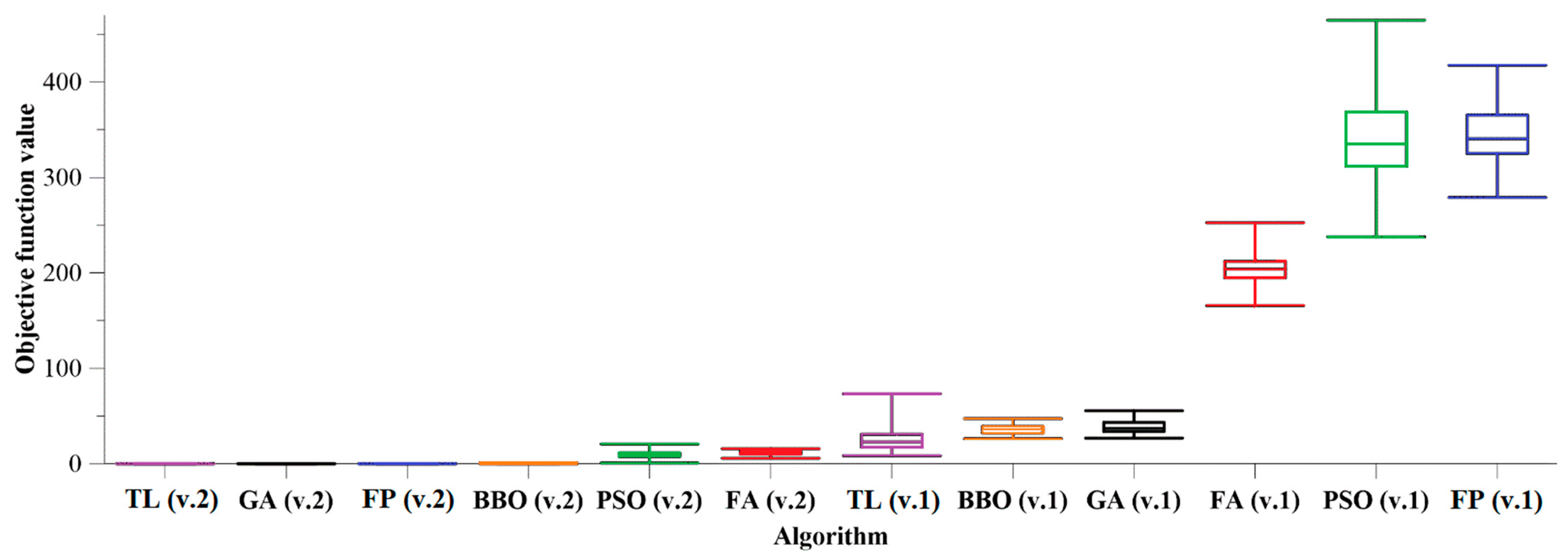
Figure 1. Box and whisker diagrams of algorithm comparison (Griewank problem).
Algorithms 15 00359 g001
Figure 2. Box and whisker diagrams of algorithms comparison (Rastrigin problem).
Algorithms 15 00359 g002
Figure 3. Box and whisker diagrams of algorithms comparison (Schwefel problem).
Algorithms 15 00359 g003
Figure 4. Box and whisker diagrams of algorithms comparison (Ackley problem).
Algorithms 15 00359 g004
Figure 5. Dependence of the best-found values on the dimension.
Algorithms 15 00359 g005
Figure 6. Trajectories obtained when solving the model identification problem.
Algorithms 15 00359 g006
Table 1. The values of algorithmic parameters.
AlgorithmValues of Parameters
FP (v.1) m = 10 ,   N L O C = 0 ,   ε b i o = 10 6 ,   P s = 0.2
FP (v.2) m = 10 ,   N L O C = 30 ,   ε b i o = 10 6 ,   P s = 0.2
TL (v.1) m = 10 ,   ε b i o = 10 6 ,   N L O C = 0
TL (v.2) m = 10 ,   ε b i o = 10 6 ,   N L O C = 30
FA (v.1) m = 10 ,   N L O C = 0 ,   ε b i o = 10 6 ,   α ˜ =   1.0 ,   β ^ 0 = 3.0 ,     γ = 0.5 ,     M = 10
FA (v.2) m = 10 ,   N L O C = 30 ,   ε b i o = 10 6 ,   α ˜ =   1.0 ,   β ^ 0 = 3.0 ,     γ = 0.5 ,     M = 10
Table 2. Statistics on algorithm launches: mean and standard deviation (SD).
AlgorithmGriewankRastriginSchwefelAckley
MeanSDMeanSDMeanSDMeanSD
FP (v.1)343.9228.532550.2128.97411,892.6648.7915.5320.2518
FP (v.2)0.04960.03062.94731.55611933.58106.954.38350.8977
TL (v.1)25.83412.927280.1627.01923,524.76213.67.11381.1376
TL (v.2)0.04460.02550.04330.02927808.612069.50.78920.2384
FA (v.1)205.3517.120818.9969.12621,146.8942.9215.8720.9408
FA (v.2)11.7132.4140265.9173.0133519.01157.436.25181.8042
GA (v.1)38.6756.5504191.9818.6225126.49544.458.10850.5020
GA (v.2)0.05360.02620.00890.0055808.21591.1870.43230.1315
BBO (v.1)36.2485.1454937.1576.52820,091.31201.310.9980.5813
BBO (v.2)0.59530.5083215.038.98583341.13200.061.94910.5387
PSO (v.1)339.3749.630937.3853.78535,812.41218.715.2010.5299
PSO (v.2)10.8014.4535269.856.23048948.39304.704.10050.5175
Table 3. The results of the numerical testing of computational technology (N = 5).
GeneratorStarterValueStarterValueStarterValue
1 (LG)Raider−83,437.0434Dichotomy−83,246.7618Polyak−80,462.6233
2 (AG)Raider−83,321.4980Dichotomy−83,247.6218Polyak−80,383.5143
3 (GG)Raider−83,543.6279Dichotomy−83,302.7432Polyak−80,516.2512
4 (LAG)Raider−83,458.6975Dichotomy−83,325.1594Polyak−80,523.4218
5 (LGG)Raider−83,459.8748Dichotomy−83,329.1129Polyak−80,524.5373
6 (AGG)Raider−83,457.2522Dichotomy−83,327.2542Polyak−80,522.6132
7 (LAGG)Raider−83,552.3954Dichotomy−83,429.4154Polyak−80,653.2337
FP (v.1)−65,293.1424TL (v.1)−65,863.6213FA (v.1)−64,571.3352
FP (v.2)−78,652.3226TL (v.2)−78,926.2372FA (v.2)−77,734.5137
Table 4. The best-found values (number of atoms: from 81 to 100).
NValueNValueNValueNValue
81−79,382.048686−84,502.632191−89,817.387596−95,046.4031
82−80,478.471187−85,627.668592−90,787.296197−96,121.8664
83−81,403.527088−86,607.611293−91,827.637598−97,165.4582
84−82,468.228689−87,689.915494−92,906.861799−98,222.4219
85−83,552.395490−88,776.599895−93,916.8247100−99,273.6113
Table 5. The changes in the trajectories of the system x ( t ) ,   y ( t ) ,   z ( t ) over time.
t012345678
x ¯ ( t ) 34.232.728.428.528.728.831.532.834.6
y ¯ ( t ) 40.338.536.734.234.434.535.736.438.2
z ¯ ( t ) 36.532.829.627.225.725.125.325.826.4
Table 6. Results of statistical testing of combined algorithms.
AlgorithmPlaces in the Ranking of Algorithms on the Collection of Test Problems
FirstSecondThirdFourthFifthSixth
GA (v.2)45.5% (10)22.7% (5)18.2% (4)13.6% (3)0.0% (0) 0.0% (0)
TL (v.2) 27.3% (6)40.9% (9)13.6% (3)4.5% (1) 9.1% (2) 4.6% (1)
FP (v.2)4.5% (1) 18.2% (4)27.3% (6)9.1% (2) 18.2% (4)22.7% (5)
BBO (v.2)4.5% (1) 13.6% (3)31.8% (7)36.4% (8)9.1% (2) 4.6% (1)
FA (v.2)13.6% (3)0.0% (0) 4.5% (1) 13.7% (3)40.9% (9)27.3% (6)
PSO (v.2)4.5% (1) 4.5% (1) 4.6% (1) 22.7% (5)22.8% (5)40.9% (9)
Publisher’s Note: MDPI stays neutral with regard to jurisdictional claims in published maps and institutional affiliations.