A Modified Liu and Storey Conjugate Gradient Method for Large Scale Unconstrained Optimization Problems

Abstract

The conjugate gradient method is one of the most popular methods to solve large-scale unconstrained optimization problems since it does not require the second derivative, such as Newton’s method or approximations. Moreover, the conjugate gradient method can be applied in many fields such as neural networks, image restoration, etc. Many complicated methods are proposed to solve these optimization functions in two or three terms. In this paper, we propose a simple, easy, efficient, and robust conjugate gradient method. The new method is constructed based on the Liu and Storey method to overcome the convergence problem and descent property. The new modified method satisfies the convergence properties and the sufficient descent condition under some assumptions. The numerical results show that the new method outperforms famous CG methods such as CG-Descent 5.3, Liu and Storey, and Dai and Liao. The numerical results include the number of iterations and CPU time.

1. Introduction

The optimization problem that we want to solve takes the following form:

$$\min f(x),x\in {ℝ}^{\mathrm{n}} ,$$

where $f$ $:{ℝ}^{\mathrm{n}}\to ℝ$ is a continuous and differentiable function, and its gradient ($\nabla f(x))$ is available.$x_1\in {ℝ}^{\mathrm{n}}$ is an arbitrary initial point for new functions or non-standard functions. The CG method generates a sequence of iterates $x_k$(vector) as follows:

Where $x_k$ is the current iteration and ${\alpha }_k>0$ is a step size obtained from a line search

$$x_{k+1}=x_k+{\alpha }_k{d}_k,k=1,2,\dots ,$$

(1)

such as exact or inexact line search. The search direction $d_k$ in the CG method requests only the first derivative of the optimization function, and it is defined as follows:

$$d_k=\{\begin{array}{l}-g_k,\\ -g_k+{\beta }_k{d}_{k-1},\end{array}\begin{array}{l}\mathrm{if}k=1,\\ \mathrm{if}k\ge 2,\end{array}$$

(2)

where $g(x)=\nabla f(x)$, $g_k=g(x_k)$ and ${\beta }_k$ is known as the CG formula or CG parameter. To obtain the step size ${\alpha }_k$, we can use the following line searches:

Exact line search, which is given by the following equation

$$f(x_k+{\alpha }_k{d}_k)=\min f(x_k+\alpha d_k),\alpha \ge 0.$$

(3)

However, Equation (3) is computationally expensive if the function has multiple local minima or stationary points.

Inexact line search, normally we use strong Wolfe–Powell (SWP) [1,2], which is defined as follows:

$$f(x_k+{\alpha }_k{d}_k)\le f(x_k)+\delta {\alpha }_k{g}_k^T{d}_k,$$

(4)

and

$$\left|g{(x_k+{\alpha }_k{d}_k)}^T{d}_k\right|\le \sigma \left|g_k^T{d}_k\right|,$$

(5)

where $0<\delta <\sigma <1$.

From Equation (4), we can note that

$$f(x_k+{\alpha }_k{d}_k)-f(x_k)\le \delta {\alpha }_k{g}_k^T{d}_k,$$

i.e.,

$$f(x_{k+1})-f(x_k)\le \delta {\alpha }_k{g}_k^T{d}_k.$$

If Equation (7) holds, then the following equation holds

$$f(x_{k+1})\le f(x_k).$$

Also, note that Equation (5) can be written as follows

$$\sigma g_k^T{d}_k\le g{(x_k+{\alpha }_k{d}_k)}^T{d}_k\le -\sigma g_k^T{d}_k.$$

Another version of Wolfe–Powell (WP) line search is the weak Wolfe–Powell (WWP) line search, which is defined by Equation (4) and the following equation

$$g{(x_k+{\alpha }_k{d}_k)}^T{d}_k\ge \sigma g_k^T{d}_k.$$

(6)

The most famous classical formulas of the CG methods are Hestenses–Stiefel (HS) [3], Polak–Ribiere–Polyak (PRP) [4], Liu and Storey (LS) [5], Fletcher–Reeves(FR) [6], Fletcher (CD) [7], as well as Dai and Yuan (DY) [8], given as follows:

$$\begin{gathered} {\beta }_k^{HS}=\frac{g_k^T{y}_{k-1}}{d_{k-1}^T{y}_{k-1}},{\beta }_k^{PRP}=\frac{g_k^T{y}_{k-1}}{{\Vert g_{k-1}\Vert }^2},{\beta }_k^{LS}=-\frac{g_k^T{y}_{k-1}}{d_{k-1}^T{g}_{k-1}} \\ {\beta }_k^{FR}=\frac{{\Vert g_k\Vert }^2}{{\Vert g_{k-1}\Vert }^2},{\beta }_k^{CD}=-\frac{{\Vert g_k\Vert }^2}{d_{k-1}^T{g}_{k-1}},{\beta }_k^{DY}=\frac{{\Vert g_k\Vert }^2}{d_{k-1}^T{g}_{k-1}}, \end{gathered}$$

where $y_{k-1}=g_k-g_{k-1}$.

The first group of classical methods, i.e., (HS), (PRP), and (LS), are efficient. However, Powell [9] proposed a counterexample to show that there exists a non-convex function. PRP, HS, and LS fail to satisfy the convergence properties even when the exact line search is used. Powell suggested the importance to achieve the convergence properties of PRP, HS, and LS methods, where the methods should be non-negative. Gilbert and Nocedal [10] showed that non-negative PRP or HS, i.e., ${\beta }_k=\max \{{\beta }_k^{HS},0\}$, is convergent under special different line searches. The second group of classical CG methods, i.e., (FR), (PRP), (DY), are robust and converge. However, the group is not efficient.

The descent condition (downhill condition) performs an important ruling in the convergence of the CG method and its robustness, which is defined as follows

$$g_k^T{d}_k<0.$$

Al–Baali [11] proposed another version of the descent condition called the sufficient descent condition, which plays a significant role in the convergence of the CG method. The author used Equation (7) to establish the convergence properties of ${\beta }_k^{FR}$, which are defined as follows: There exists a constant $c>0$ such that

$$g_k^T{d}_k\le -c{\Vert g_k\Vert }^2,\forall k\in N.$$

(7)

In this case, the function is quadratic, i.e., $f(x)=g^{T}x+(1/2)x^{T}Hx$ and the step size obtained by exact line search (3) indicates that the CG method satisfies the conjugacy condition, i.e., $d_i^{T}H{d}_j^T=0,$ $\forall i\ne j$. Using the mean value theorem and exact line search of Equation (2), we can obtain ${\beta }_k^{HS}$. From the quasi-Newton method, BFGS method, the limited memory (LBFGS) method, and using Equation (2), Dai and Liao [12] proposed the following conjugacy condition.

$$d_k^T{y}_{k-1}=-t{g}_k^T{s}_{k-1},$$

(8)

where $s_{k-1}=x_k-x_{k-1},$ and $t\ge 0,$ [12] use $t=0.1$ in the numerical experiments. In the case of $t=0$, Equation (8) becomes the classical conjugacy condition. By using Equations (2) and (8), Dai and Liao [12] proposed the following CG formula

$${\beta }_k^{DL}=\frac{g_k^T{y}_{k-1}}{d_{k-1}^T{y}_{k-1}}-t\frac{g_k^T{s}_{k-1}}{d_{k-1}^T{y}_{k-1}}.$$

(9)

However, ${\beta }_k^{DL}$ face the same problem as ${\beta }_k^{PRP}$ and ${\beta }_k^{HS}$, i.e., ${\beta }_k^{DL}$ is not non-negative in general. Thus, Dai and Liao [12] replaced Equation (9) by

$${\beta }_k^{DL+}=\max \{{\beta }_k^{HS},0\}-t\frac{g_k^T{s}_{k-1}}{d_{k-1}^T{y}_{k-1}}.$$

(10)

Hager and Zhang [13,14] presented a modified CG parameter that satisfies the descent property for any inexact line search with $g_k^T{d}_k\le -(7/8){\Vert g_k\Vert }^2$. This new version of the CG method is convergent whenever the line search satisfies the WP line search. This formula is given as follows:

$${\beta }_k^{HZ}=\max \{{\beta }_k^N,{\eta }_k\}$$

(11)

where ${\beta }_k^N=\frac{1}{d_k^T{y}_k}{(y_k-2d_k\frac{{\Vert y_k\Vert }^2}{d_k^T{y}_k})}^T{g}_k$, ${\eta }_k=-\frac{1}{\Vert d_k\Vert \min \{\eta ,\Vert g_k\Vert \}}$, and $\eta >0$ is a constant.

Note that if $t=2\frac{{\Vert y_k\Vert }^2}{s_k^T{y}_k}$, then ${\beta }_k^N={\beta }_k^{DY}.$ Zhang et al. [15] and Zhang and Xu [16] used Taylor’s series and presented the following modified secant relation:

$$\begin{gathered} B_k{s}_{k-1}={\overline{y}}_{k-1}\mathrm{where}{\overline{y}}_{k-1}=y_{k-1}+\frac{{\vartheta }_{k-1}}{{\Vert s_{k-1}\Vert }^2}{s}_k\mathrm{and} \\ {\vartheta }_{k-1}=6(f_{k-1}-f_k)+3{(g_{k-1}+g_k)}^T{s}_{k-1}. \end{gathered}$$

(12)

From (12), Yabe and Takano [17] proposed the following formula:

$${\beta }_k^{YT}=\frac{g_k^T(z_{k-1}-t{s}_{k-1})}{d_{k-1}^T{z}_{k-1}}\mathrm{where}{z}_{k-1}=y_{k-1}+\rho \frac{{\vartheta }_{k-1}}{{\Vert s_{k-1}\Vert }^2}{s}_k\mathrm{and}\rho \ge 0.$$

(13)

Moreover, Razieh Dehghani et al. [18] proposed the following formula:

$${\beta }_k^{YT}=\frac{g_k^T(y_{k-1}^{*}-t{s}_{k-1})}{d_{k-1}^T{y}_{k-1}^{*}}.$$

(14)

Jiang et al. [19] proposed the CG method by replacing $d_{k-1}$ by $g_{k-1}$ in ${\beta }_k^{HS}$ as follows:

$${\beta }_k^{JJSL}=\frac{g_k^T{y}_{k-1}}{g_{k-1}^T{y}_{k-1}}.$$

Furthermore, Wei et al. [20] proposed a non-negative formula, referred to as the WYL coefficient. It is defined as follows:

$${\beta }_k^{WYL}=\frac{{\Vert g_k\Vert }^2-\frac{\Vert g_k\Vert }{\Vert g_{k-1}\Vert }{g}_k^T{g}_{k-1}^{}}{{\Vert g_{k-1}\Vert }^2}$$

This parameter is similar to the PRP coefficient, which possesses convergence with both an exact line and inexact line searches, providing a sufficient descent condition. Many modifications of the WYL coefficient have been suggested. The reader can refer to [21]. Here we mention some of them.

$${\beta }_k^{VHS}=\frac{{\Vert g_k\Vert }^2-\frac{\Vert g_k\Vert }{\Vert g_{k-1}\Vert }{g}_k^T{g}_{k-1}^{}}{d_{k-1}^T(g_k^{}-g_{k-1})}\mathrm{and}{\beta }_k^{NPRP}=\frac{{\Vert g_k\Vert }^2-\frac{\Vert g_k\Vert }{\Vert g_{k-1}\Vert }\left|g_k^T{g}_{k-1}\right|}{{\Vert g_{k-1}\Vert }^2},$$

which were presented in [22,23], respectively.

Al-Baali et al. [24] proposed a new CG version called (G3TCG) that offers many selections of CG parameters. The same study [24] found that the G3TCG method is more efficient than ${\beta }_k^{HZ}$ in some cases and competitive in some other cases.

The convergence rate for the CG method is linear unless the iterative procedure is occasionally restarted at least every $n$ iterations [25]. Beale [26] suggested the use of the two-term CG method instead of the steepest descent (SD) method ($d_k=-g_k,\forall k\ge 1)$ as the restart search direction. He also extended this method to a three-term method as a non-restart direction. Furthermore, Powell [25] suggested restarting the search direction using Beale’s method if

$$\left|g_k^T{g}_{k-1}\right|>0.2{\Vert g_k\Vert }^2,$$

holds for every $n$ iteration, whichever first occurs. Dai and Yuan [27] extended the Powell restart criteria (7) to the following form

$$\left|g_k^T{g}_{k-1}\right|>\tau {\Vert g_k\Vert }^2,\dots \tau \in (0,1).$$

Besides, Alhawarat et al. [28] presented the following simple formula

$${\beta }_k^{AZPRP}=\{\begin{array}{l}\frac{{\Vert g_k\Vert }^2-{\mu }_k\left|g_k^T{g}_{k-1}\right|}{{\Vert g_{k-1}\Vert }^2},\mathrm{if}{\Vert g_k\Vert }^2>{\mu }_k\left|g_k^T{g}_{k-1}\right|,\\ 0,\mathrm{otherwise},\end{array}$$

(15)

where $\Vert \cdot \Vert$ represents the Euclidean norm and ${\mu }_k$ is defined as follows:

$${\mu }_k=\frac{\Vert x_k-x_{k-1}\Vert }{\Vert y_k\Vert }$$

Lemma 3.1 in [28] shows that if Assumption 1 holds and the Beale–Powell restart condition is violated for non-restart search direction, then ${\Vert g_k\Vert }^2>{\mu }_k\left|g_k^T{g}_{k-1}\right|$ holds.

Moreover, Kaelo et al. [29] proposed a non-negative CG formula with convergence properties, and compared the new formula with ${\beta }_k^{AZPRP}$, where the proposed method is given as follows:

$${\beta }_k^{PKT}=\{\begin{array}{l}\frac{{\Vert g_k\Vert }^2-g_k^T{g}_{k-1}}{\max \{d_{k-1}^T{y}_{k-1},-g_{k-1}^T{d}_{k-1}\}},\mathrm{If}0<g_k^T{g}_{k-1}<{\Vert g_k\Vert }^2\\ \frac{{\Vert g_k\Vert }^2}{\max \{d_{k-1}^T{y}_{k-1},-g_{k-1}^T{d}_{k-1}\}},\mathrm{otherwise}.\end{array}$$

To solve non-linear monotone equations with convex constraints, [30] proposed using the Powell symmetrical technique to the Liu–Storey conjugate gradient method. The reader can refer to the references for more about non-linear monotone equations with convex constraints and their application [31,32,33,34].

2. The Proposed CG Formula and Its Motivation

The CG method with ${\beta }_k^{LS}$ cannot satisfy the decent condition. On the other hand, ${\beta }_k^{LS}$ comes from the group of efficient CG method as explained before to inherit the efficiency of ${\beta }_k^{LS}$. To avoid the convergence problem, we use ${\beta }_k^{AZPRP}$ in [19] and ${\beta }_k^{DL}$ in [12] to propose a new non-negative CG method that satisfies the sufficient descent condition with SWP line search. Moreover, convergence properties are achieved. The new formula is a modification of ${\beta }_k^{LS}$,${\beta }_k^{DL}$, and ${\beta }_k^{AZPRP}$ defined as follows:

$${\beta }_k^{LS+}=\{\begin{array}{l}-\frac{{\Vert g_k\Vert }^2-{\mu }_k\left|g_k^T{g}_{k-1}\right|}{d_{k-1}^T{g}_{k-1}}\mathrm{if}{\Vert g_k\Vert }^2>{\mu }_k\left|g_k^T{g}_{k-1}\right|,\\ {\beta }_k^{DL-HS}\mathrm{otherwise}\end{array}$$

(16)

where $\Vert \cdot \Vert$ represents the Euclidean norm and

$${\beta }_k^{DL-HS}=-{\mu }_k\frac{g_k^T{s}_{k-1}}{d_{k-1}^T{y}_{k-1}}.$$

The proposed method in Equation (16) has the following attitudes:

• Satisfies the descent condition.
• Satisfies the convergence properties.
• Equation (16) is constructed based on ${\beta }_k^{LS}$ with restart condition to be non-negative and avoid the convergence problems.
• Dai and Liao [12] suggest using $-t\left(g_k^T{s}_{k-1}/d_{k-1}^T{y}_{k-1}\right)$ instead of steepest descent as a restart criterion, where Equation (16) is restarted by $-{\mu }_k\left(g_k^T{s}_{k-1}/d_{k-1}^T{y}_{k-1}\right)$, more efficient than the steepest descent.
• The numerical results demonstrate the efficiency and robustness of Equation (16) compared to the other CG methods, including CG-Descent, LS, and DL+.

3. Convergence Analysis of ${\beta }_k^{LS+}$

In the analysis below, we obtain the stationary point from the convergence mean. In addition, if $g_k=$$0$, then a stationary point has been obtained. Thus, we assume $g_k\ne$$0$ for all $k\ge 1$ in the subsequent analysis. For more about local and global minimum points, the reader can refer to the following useful references [35,36].

To satisfy the convergence analysis of the modified CG method, the following assumption is required.

Assumption 1. 

A. The level set$\Phi =\left\{x|f(x)\le f(x_1)\right\}$is bounded; that is, a positive constant$\lambda$exists such that

$$\Vert x\Vert \le \lambda ,\forall x\in \Phi .$$

B. In some neighborhood${\rm P}$of$\Phi$,$f$is continuously differentiable, and its gradient is Lipschitz continuous; that is, for all$x,y\in {\rm P},$there exists a constant$L>0$such that

$$\Vert g(x)-g(y)\Vert \le L\Vert x-y\Vert$$

This assumption implies that there exists a positive constant$\overline{\gamma }$such that

$$\Vert g(x)\Vert \le \overline{\gamma },\forall x\in {\rm P}.$$

The following algorithm (Algorithm 1) classifies the steps of the CG method to obtain the stationary point using Equation (16) and SWP line search.

Algorithm 1. The steps to obtain the optimum point of optimization problem by using the CG method

Step 1 Provide a starting point $x_1.$ Set the initial search direction $d_1=-g_1$. Let $k=1$.

Step 2 If a stopping criteria is satisfied, then stop.

Step 3 Compute $d_k$ based on (2) with (16).

Step 4 Compute ${\alpha }_k$ using (4) and (5).

Step 5 Update $x_{k+1}.$ based on (1).

Step 6 Set $k:=k+1$ and go to Step 2.

In the following section and subsections, we obtain the descent condition and the convergence property of Equation (16) with CG formula, the proof similar to that presented by [12].

3.1. The Descent Property of CG Method with ${\beta }_k^{LS+}$

Theorem 1. 

Let the sequences$\left\{x_k\right\}$and$\left\{d_k\right\}$be obtained using (1), (2), and${\beta }_k^{LS+}$, where${\alpha }_k$is computed using the SWP line search (4) and (5). If$\sigma \in (0,\frac{1}{2}]$, then the descent condition given in (7) holds.

Proof. 

By multiplying (2) by $g_k^T,$ we obtain

$$\begin{gathered} g_k^T{d}_k=g_k^T(-g_k^{}+{\beta }_k{d}_{k-1})=-{\Vert g_k\Vert }^2+{\beta }_k{g}_k^T{d}_{k-1} \\ =-{\Vert g_k\Vert }^2+\left(-\frac{{\Vert g_k\Vert }^2-{\mu }_k\left|g_k^T{g}_{k-1}\right|}{d_{k-1}^T{g}_{k-1}}\right)g_k^T{d}_{k-1}. \end{gathered}$$

(17)

By using the proof by induction technique, for $k=1,$ it is true, i.e., $g_{{}_1}^T{d}_1=-{\Vert g_1\Vert }^2$. We now assume that it is true until $k-1,$ thus we can write Equation (16) as follows:

$${\beta }_k^{LS+}=\frac{-{\Vert g_k\Vert }^2+{\mu }_k\left|g_k^T{g}_{k-1}\right|}{d_{k-1}^T{g}_{k-1}}\le \frac{-{\Vert g_k\Vert }^2}{d_{k-1}^T{g}_{k-1}}+\frac{{\mu }_k\left|g_k^T{g}_{k-1}\right|}{d_{k-1}^T{g}_{k-1}}\le \frac{-{\Vert g_k\Vert }^2}{d_{k-1}^T{g}_{k-1}}=\frac{{\Vert g_k\Vert }^2}{{\Vert g_{k-1}\Vert }^2}$$

Divide both sides of Equation (18) by ${\Vert g_k\Vert }^2$ and using (5), we obtain

$$-1+\sigma \frac{g_{k-1}^T{d}_{k-1}}{\left|\right|g_{k-1}|{|}^2}\le \frac{g_k^T{d}_k}{\left|\right|g_k|{|}^2}\le -1-\sigma \frac{g_{k-1}^T{d}_{k-1}}{\left|\right|g_{k-1}|{|}^2}.$$

(18)

Repeating the process for the left-hand side of Equation (18), we obtain

$$-1+{\displaystyle \sum _{j=1}^{k-1}{\sigma }^j}=-{\displaystyle \sum _{j=0}^{k-1}{\sigma }^j}.$$

Repeating the process for the right hand side of Equation (18) yields

$$-1-{\displaystyle \sum _{j=1}^{k-1}{\sigma }^j}=-2+{\displaystyle \sum _{j=0}^{k-1}{\sigma }^j}.$$

Thus, Equation (18) can be written as follows:

$$-{\displaystyle \sum _{j=0}^{k-1}{\sigma }^j}\le \frac{g_k^T{d}_k}{\left|\right|g_k|{|}^2}\le -2+{\displaystyle \sum _{j=0}^{k-1}{\sigma }^j}$$

Since

$${\displaystyle \sum _{j=0}^{k-1}{(\sigma )}^j<}\frac{1-{(\sigma )}^k}{1-\sigma },$$

hence

$$-\frac{1-{(\sigma )}^k}{1-\sigma }\le \frac{g_k^T{d}_k}{\left|\right|g_k|{|}^2}\le -2+\frac{1-{(\sigma )}^k}{1-\sigma }.$$

When $\sigma \le 1/2$, we obtain $\frac{1-{(\sigma )}^k}{1-\sigma }<2$. Let $c=2-\frac{1-{(\sigma )}^k}{1-\sigma }$, then

$$c-2\le \frac{g_k^T{d}_k}{\left|\right|g_k|{|}^2}\le -c.$$

(19)

The proof is complete. □

3.2. The Convergence Property of the CG Method with ${\beta }_k^{LS+}$ to Obtain the Stationary Point

Theorem 2. 

Let Assumption 1 hold. Consider any form of (1) and (2), with the new formula (10), in which${\alpha }_k$is obtained from the SWP line search (4) and (5) with$\sigma \le 1/2.$Then,

$$\underset{k\to \infty }{\lim \inf }\Vert g_k\Vert =0.$$

Proof. 

We will prove the theorem by contradiction. Assume that the conclusion is not true.

Then, a constant $\epsilon >0$ exists such that

$$\Vert g_k\Vert \ge \epsilon ,\forall k\ge 1.$$

(20)

Upon squaring both sides of (2), we obtain

$${\Vert d_k\Vert }^2={\Vert g_k\Vert }^2-2{\beta }_k{g}_k^T{d}_{k-1}+{\beta }_k^2{\Vert d_{k-1}\Vert }^2.$$

(21)

Dividing Equation (21) by ${\Vert g_k\Vert }^4$ yields

$$\frac{{\Vert d_k\Vert }^2}{{\Vert g_k\Vert }^4}=\frac{1}{{\Vert g_k\Vert }^2}-\frac{2{\beta }_k{g}_k^T{d}_{k-1}}{{\Vert g_k\Vert }^4}+\frac{{\beta }_k^2{\Vert d_{k-1}\Vert }^2}{{\Vert g_k\Vert }^4}.$$

Using Equations (5) and (16), we now obtain

$$\frac{{\Vert d_k\Vert }^2}{{\Vert g_k\Vert }^4}\le \frac{{\Vert d_{k-1}\Vert }^2}{{\Vert g_{k-1}\Vert }^4}+\frac{1}{{\Vert g_k\Vert }^2}+\frac{2\sigma \left|g_{k-1}^T{d}_{k-1}\right|}{{\Vert g_{k-1}\Vert }^2{\Vert g_k\Vert }^2}\le \frac{{\Vert d_{k-1}\Vert }^2}{{\Vert g_{k-1}\Vert }^4}+\frac{1+2\sigma (2-c)}{{\Vert gk\Vert }^2}.$$

(22)

Repeating the process for (22) using the relationship $\frac{1}{\Vert g_1\Vert }=\frac{1}{\Vert d_1\Vert }$ yields

$$\frac{{\Vert d_k\Vert }^2}{{\Vert g_k\Vert }^4}\le (1+2\sigma (2-c)){\displaystyle \sum _{i=1}^k\frac{1}{{\Vert g_i\Vert }^2}}$$

From (20), we obtain

$$\frac{{\Vert g_k\Vert }^4}{{\Vert d_k\Vert }^2}\ge \frac{{\epsilon }^2}{k(1+2\sigma (2-c))}$$

Therefore,

$${\displaystyle \sum _{k=0}^{\infty }\frac{{\Vert g_k\Vert }^4}{{\Vert d_k\Vert }^2}=\infty }.$$

 □

Theorem 3. 

Suppose the sequences$\left\{x_k\right\}$and$\left\{d_k\right\}$are obtained by using (1), (2), and${\beta }_k^{DL-HS}$, where${\alpha }_k$is computed via the SWP line search (4) and (5). Then, the descent condition holds.

Proof. 

Let

$${\beta }_k^{DL-HS}=-{\mu }_k\frac{g_k^T{s}_{k-1}}{d_{k-1}^T{y}_{k-1}}.$$

By multiplying (2) by $g_k^T,$ and substituting ${\beta }_k^{DL-HS}$, we obtain

$$g_k^T{d}_k=-{\Vert g_k\Vert }^2-{\mu }_k\frac{{\alpha }_{k-1}{g}_k^T{d}_{k-1}}{d_{k-1}^T{y}_{k-1}}{g}_k^T{d}_{k-1}.$$

$$g_k^T{d}_k=-{\Vert g_k\Vert }^2-{\mu }_k\frac{{\alpha }_{k-1}{\Vert g_k^T{d}_{k-1}\Vert }^2}{d_{k-1}^T{y}_{k-1}}<0.$$

This completes the proof. □

The condition in (23) is called Zoutendijk condition [37], acting as an important role in proving convergence properties of the CG method.

Lemma 1. 

Assume that Assumption 1 holds. Consider any form of (1) and (2) with step size${\alpha }_k$satisfying the WWP line search, where the search direction$d_k$is descent. Then, we have

$${\displaystyle \sum _{k=0}^{\infty }\frac{{(g_k^T{d}_k)}^2}{{\Vert d_k\Vert }^2}}<\infty .···$$

(23)

Moreover, (23) holds for exact and SWP line searches. Substituting (7) into (18), it follows that

$${\displaystyle \sum _{k=0}^{\infty }\frac{{\Vert g_k\Vert }^4}{{\Vert d_k\Vert }^2}}<\infty .···$$

(24)

Theorem 4. 

Assume that Assumption 1 holds. Consider the conjugate gradient method in (1) and (2) with${\beta }_k^{DL-HS}$, where$d_k$is a descent direction and${\alpha }_k$is obtained by the strong Wolfe line search. Then, the$\underset{k\to \infty }{\lim \inf }\Vert g_k\Vert =0.$

Proof. 

We will prove this theorem by contradiction. Suppose Theorem 4 is not true.

Then, a constant $\epsilon >0$ exists such that

$$\Vert g_k\Vert \ge \epsilon ,\forall k\ge 1.$$

(25)

By squaring both sides of (2), we obtain

$$\begin{array}{l}{\Vert d_k\Vert }^2={\Vert g_k\Vert }^2-2{\beta }_k{g}_k^T{d}_{k-1}+{\beta }_k^2{\Vert d_{k-1}\Vert }^2\\ \le {\Vert g_k\Vert }^2+2\left|{\beta }_k\right|g_k^T{d}_{k-1}+{\beta }_k^2{\Vert d_{k-1}\Vert }^2\\ \le {\Vert g_k\Vert }^2+\frac{2}{L}\frac{\Vert g_k\Vert \Vert s_k\Vert }{(1-\sigma )g_{k-1}^T{d}_{k-1}}\left(\sigma \right)g_{k-1}^T{d}_{k-1}+\frac{1}{L^2}\frac{{\left(\left(\sigma \right)g_{k-1}^T{d}_{k-1}\right)}^2{\Vert s_{k-1}\Vert }^2}{(1-\sigma )g_{k-1}^T{d}_{k-1}}\\ \le {\Vert g_k\Vert }^2+\frac{2}{L}\frac{\Vert g_k\Vert \Vert s_k\Vert }{(1-\sigma )}\sigma +\frac{1}{L^2}\frac{{\left(\sigma \right)}^2{\Vert s_{k-1}\Vert }^2}{{(1-\sigma )}^2}.\\ \frac{{\Vert d_k\Vert }^2}{{\Vert g_k\Vert }^4}\le \frac{{\Vert g_k\Vert }^2}{{\Vert g_k\Vert }^4}+\frac{2}{L}\frac{\Vert g_k\Vert \Vert s_k\Vert }{(1-\sigma ){\Vert g_k\Vert }^4}\sigma +\frac{1}{L^2}\frac{{\sigma }^2{\Vert s_{k-1}\Vert }^2}{{(1-\sigma )}^2{\Vert g_k\Vert }^4}\\ \le \frac{1}{{\Vert g_k\Vert }^2}+\frac{2}{L}\frac{\Vert g_k\Vert \Vert s_k\Vert }{(1-\sigma ){\Vert g_k\Vert }^4}\sigma +\frac{1}{L^2}\frac{{\sigma }^2{\Vert s_{k-1}\Vert }^2}{{(1-\sigma )}^2{\Vert g_k\Vert }^4}.\\ \le \frac{1}{{\Vert g_k\Vert }^2}+\frac{2}{L}\frac{\Vert s_k\Vert }{(1-\sigma ){\Vert g_k\Vert }^3}\sigma +\frac{1}{L^2}\frac{{\sigma }^2{\Vert s_{k-1}\Vert }^2}{{(1-\sigma )}^2{\Vert g_k\Vert }^4}.\end{array}$$

Let

$${\Vert g_k\Vert }^m=\min \left\{{\Vert g_k\Vert }^2,{\Vert g_k\Vert }^3,{\Vert g_k\Vert }^4\right\},m\in N$$

then

$$\frac{{\Vert d_k\Vert }^2}{{\Vert g_k\Vert }^4}\le \frac{1}{{\Vert g_k\Vert }^m}\left(1+\frac{2}{L}\frac{\lambda }{(1-\sigma )}\sigma +\frac{1}{{\lambda }^2}\frac{{\sigma }^2{\lambda }^2}{{(1-\sigma )}^2}\right).$$

Also, let

$$R=\left(1+\frac{2}{L}\frac{\Gamma }{(1-\sigma )}\sigma +\frac{1}{{\lambda }^2}\frac{{\sigma }^2{\Gamma }^2}{{(1-\sigma )}^2}\right)$$

then

$$\begin{gathered} \frac{{\Vert d_k\Vert }^2}{{\Vert g_k\Vert }^4}\le \frac{R}{{\Vert g_k\Vert }^m}\le R{\displaystyle \sum _{i=1}^k\frac{1}{{\Vert g_i\Vert }^m}} \\ \frac{{\Vert g_k\Vert }^4}{{\Vert d_k\Vert }^2}\ge \frac{{\epsilon }^m}{kR}. \end{gathered}$$

Therefore,

$${\displaystyle \sum _{k=0}^{\infty }\frac{{\Vert g_k\Vert }^4}{{\Vert d_k\Vert }^2}=\infty }.$$

This result contradicts (24). Therefore, $\underset{k\to \infty }{\lim \inf }\Vert g_k\Vert =0.$, completing the proof. □

4. Numerical Results and Discussion

To improve the efficiency of the proposed CG method, we modified Equation (16) as follows:

$${\beta }_k^{LS+}=\{\begin{array}{l}-\frac{{\Vert g_k\Vert }^2-\left|g_k^T{g}_{k-1}\right|}{d_{k-1}^T{g}_{k-1}}\mathrm{if}{\Vert g_k\Vert }^2>\left|g_k^T{g}_{k-1}\right|\\ -\frac{{\Vert g_k\Vert }^2-{\mu }_k\left|g_k^T{g}_{k-1}\right|}{d_{k-1}^T{g}_{k-1}}\mathrm{if}{\Vert g_k\Vert }^2>{\mu }_k\left|g_k^T{g}_{k-1}\right|\\ -{\mu }_k\frac{g_k^T{s}_{k-1}}{d_{k-1}^T{y}_{k-1}}\mathrm{otherwise}\end{array}$$

To analyze the efficiency of the new formula, we selected several test problems in Appendix A from CUTEr [38]. We compared the CG-Descent, LS, DL+ coefficients based on the CPU time and the number of iterations. We employed the modified CG descent 6.8 [39] with the SWP line search with $\delta =0.01$, $\sigma =0.1$ and memory = 0 for LS, LS+, DL+ algorithms. To obtain the result of CG-Descent 5.3, we employ the CG-descent 6.3 with memory = 0. The norm of the gradient was employed as the stopping criterion, specifically $\Vert g_k\Vert \le {10}^{-6}$ for all algorithms. The host computer is an AMD A4 and 4GB of RAM. The results are shown in Figure 1 and Figure 2. Note that a performance measure introduced by Dolan and More [40] was employed. This performance measure was introduced to compare a set of solvers S on a set of problems $\rho$. Assuming $n_s$ solvers and $n_p$ problems in S and $\rho$, respectively, the measure $t_{p,s}$ is defined as the computation time (e.g., the number of iterations or the CPU time) required for the solver $s$ to solve the problem $p$.

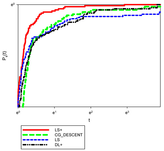
Figure 1. Performance measure based on the number of iterations.

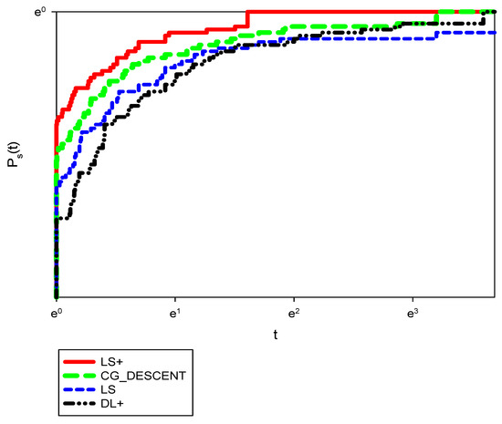
Figure 2. Performance measure based on the CPU time.

To create a baseline for comparison, the performance of the solver $s$ on the problem $p$ is scaled by the best performance of any solver in S on the problem using the ratio

$$r_{p,s}=\frac{t_{p,s}}{\min \{t_{p,s}:s\in S\}}$$

Let the parameter $r_M\ge r_{p,s}$ for all $p,s$ be selected. A further assumption made is that $r_{p,s}=r_M$ if and only if the solver $s$ does not solve the problem $p$. As we would like to obtain an overall assessment of the performance of a solver, we defined the following measure

$$P_s(t)=\frac{1}{n_p}\mathrm{size}\{p\in \rho :r_{p,s}\le t\}$$

Thus, $P_s(t)$ is the probability for a solver $s\in S$ that the performance ratio $r_{p,s}$ is within a factor $t\in R$ of the best possible ratio. Suppose we define the function $p_s$ as the cumulative distribution function for the performance ratio. In that case, the performance measure $P_s:ℝ\to [0,1]$ for a solver is non-decreasing and piecewise continuous from the right. The value of $p_s(1)$ is the probability that the solver achieves the best performance of all the solvers. In general, a solver with high values of $P_s(t)$, which would appear in the upper right corner of the figure, is preferable.

Figure 1 shows that LS+ outperforms CG-Descent 5.3, LS, and DL+ in the number of iterations. It is worth noting that LS fails to obtain the stationary point for some functions. Thus, it solves around 95% of test functions. According to Figure 2, which presents the CPU time, we note that the LS+ also outperforms CG-Descent, LS, and DL+. Also, we can note that CG-Descent outperforms DL+ and LS+ in both figures. Thus, the proposed method is more efficient than DL+ and CG-Descent and more efficient and robust than the original LS. Also, it is worth noting that the proposed method can be extended to a three term CG method by using a modified DL+ CG formula, which is our new paper in near future.

5. Conclusions

In this paper, we proposed a modification of the Liu and Storey CG method that satisfies the following main challenges:

• The proposed method is a non-negative two-term CG method.
• The proposed method satisfies the descent condition.
• The convergences properties are satisfied by obtaining the stationary point/s.
• The modified method was restarted based on the suggestion presented by [12] instead of using the steepest descent, improving the efficiency of the proposed method.
• The numerical results show that the new method outperformed CG-Descent, DL+, and LS in terms of the number of iteration and CPU time. Moreover, the modified method is more robust than the original LS.

In future, we will try to improve the line search to reduce the number of function evaluations and the number of gradient evaluations. As an application of the CG method in image restoration, the reader can refer to [41]. In addition, we will focus on some applications of the CG method, such as machine learning, deep learning, and image restoration. The proposed method is of great interest in solving nonlinear coefficient inverse problems for partial differential equations, for more, the reader can refer to the following references [42,43,44,45,46,47].

References

- Wolfe, P. Convergence Conditions for Ascent Methods. SIAM Rev. 1969, 11, 226–235. [Google Scholar] [CrossRef]
- Wolfe, P. Convergence Conditions for Ascent Methods. II: Some Corrections. SIAM Rev. 1971, 13, 185–188. [Google Scholar] [CrossRef]
- Hestenes, M.; Stiefel, E. Methods of conjugate gradients for solving linear systems. J. Res. Natl. Inst. Stand. Technol. 1952, 49, 409. [Google Scholar] [CrossRef]
- Elijah, P.; Ribiere, G. Note sur la convergence de méthodes de directions conjuguées. ESAIM: Math. Model. Numer. Anal. Modélisation Mathématique Et Anal. Numérique 1969, 3. R1, 35–43. [Google Scholar]
- Liu, Y.; Storey, C. Efficient generalized conjugate gradient algorithms, part 1: Theory. J. Optim. Theory Appl. 1991, 69, 129–137. [Google Scholar] [CrossRef]
- Fletcher, R.; Reeves, C.M. Function minimization by conjugate gradients. Comput. J. 1964, 7, 149–154. [Google Scholar] [CrossRef] [Green Version]
- Fletcher, R. Practical Methods of Optimization, Unconstrained Optimization; Wiley: New York, NY, USA, 1987. [Google Scholar]
- Dai, Y.H.; Yuan, Y. A non-linear conjugate gradient method with a strong global convergence property. SIAM J. Optim. 1999, 10, 177–182. [Google Scholar] [CrossRef] [Green Version]
- Powell, M.J.D. Non-convex minimization calculations and the conjugate gradient method, Numerical Analysis (Dundee, 1983). In Lecture Notes in Mathematics; Springer: Berlin, Germany, 1984; Volume 1066, pp. 122–141. [Google Scholar]
- Gilbert, J.C.; Nocedal, J. Global convergence properties of conjugate gradient methods for optimization. Siam. J. Optim. 1992, 2, 21–42. [Google Scholar] [CrossRef] [Green Version]
- Al-Baali, M. Descent property and global convergence of the Fletcher-Reeves method with inexact line search. IMA J. Numer. Anal. 1985, 5, 121–124. [Google Scholar] [CrossRef]
- Dai, Y.H.; Liao, L.Z. New conjugacy conditions and related non-linear conjugate gradient methods. Appl. Math. Optim. 2001, 43, 87–101. [Google Scholar] [CrossRef]
- Hager, W.W.; Zhang, H. A new conjugate gradient method with guaranteed descent and an efficient line search. Siam. J. Optim. 2005, 16, 170–192. [Google Scholar] [CrossRef] [Green Version]
- Hager, W.W.; Zhang, H. The limited memory conjugate gradient method. Siam. J. Optim. 2013, 23, 2150–2168. [Google Scholar] [CrossRef] [Green Version]
- Zhang, J.Z.; Deng, N.Y.; Chen, L.H. New quasi-Newton equation and related methods for unconstrained optimization. J. Optim. Theory Appl. 1999, 102, 147–167. [Google Scholar] [CrossRef]
- Zhang, J.Z.; Xu, C.X. Properties and numerical performance of quasi-Newton methods with modified quasi-Newton equation. J. Comput. Appl. Math. 2001, 137, 269–278. [Google Scholar] [CrossRef] [Green Version]
- Yabe, H.; Takano, M. Global convergence properties of non-linear conjugate gradient methods with modified secant relation. Comput. Optim. Appl. 2004, 28, 203–225. [Google Scholar] [CrossRef]
- Dehghani, R.; Bidabadi, N.; Fahs, H.; Hosseini, M.M. A Conjugate Gradient Method Based on a Modified Secant Relation for Unconstrained Optimization. Numer. Funct. Anal. Optim. 2020, 41, 621–634. [Google Scholar] [CrossRef]
- Jiang, X.; Jian, J.; Song, D.; Liu, P. An improved Polak–Ribière–Polyak conjugate gradient method with an efficient restart direction. Comput. Appl. Math. 2021, 40, 1–24. [Google Scholar] [CrossRef]
- Wei, Z.; Yao, S.; Liu, L. The convergence properties of some new conjugate gradient methods. Appl. Math. Comput. 2006, 183, 1341–1350. [Google Scholar] [CrossRef]
- Qu, A.; Li, M.; Xiao, Y.; Liu, J. A modified Polak–Ribi’e re–Polyak descent method for unconstrained optimization. Optim. Methods Softw. 2014, 29, 177v188. [Google Scholar] [CrossRef]
- Shengwei, Y.; Wei, Z.; Huang, H. A note about WYL’s conjugate gradient method and its applications. Appl. Math. Comput. 2007, 191, 381–388. [Google Scholar] [CrossRef]
- Zhang, L. An improved Wei–Yao–Liu non-linear conjugate gradient method for optimization computation. Appl. Math. Comput. 2009, 215, 2269–2274. [Google Scholar]
- Al-Baali, M.; Narushima, Y.; Yabe, H. A family of three-term conjugate gradient methods with sufficient descent property for unconstrained optimization. Comput. Optim. Appl. 2015, 60, 89–110. [Google Scholar] [CrossRef]
- Powell, M.J.D. Restart procedures for the conjugate gradient method. Math. Program. 1977, 12, 241–254. [Google Scholar] [CrossRef]
- Beale, E.M.L. A derivative of conjugate gradients. In Numerical Methods for Nonlinear Optimization; Lootsma, F.A., Ed.; Academic Press: London, UK, 1972; pp. 39–43. [Google Scholar]
- Dai, Y.; Yuan, Y. Convergence properties of Beale-Powell restart algorithm. Sci. China Ser. A Math. 1998, 41, 1142–1150. [Google Scholar] [CrossRef]
- Alhawarat, A.; Salleh, Z.; Mamat, M.; Rivaie, M. An efficient modified Polak–Ribière–Polyak conjugate gradient method with global convergence properties. Optim. Methods Softw. 2017, 32, 1299–1312. [Google Scholar] [CrossRef]
- Kaelo, P.; Mtagulwa, P.; Thuto, M.V. A globally convergent hybrid conjugate gradient method with strong Wolfe conditions for unconstrained optimization. Math. Sci. 2019, 14, 1–9. [Google Scholar] [CrossRef] [Green Version]
- Liu, J.K.; Xu, J.Ł.; Zhang, L.Q. Partially symmetrical derivative-free Liu–Storey projection method for convex constrained equations. Int. J. Comput. Math. 2019, 96, 1787–1798. [Google Scholar] [CrossRef]
- Gao, P.; He, C.; Liu, Y. An adaptive family of projection methods for constrained monotone non-linear equations with applications. Appl. Math. Comput. 2019, 359, 1–16. [Google Scholar]
- Zheng, L.; Yang, L.; Liang, Y. A Modified Spectral Gradient Projection Method for Solving Non-linear Monotone Equations with Convex Constraints and Its Application. IEEE Access 2020, 92677–92686. [Google Scholar] [CrossRef]
- Zheng, L.; Yang, L.; Liang, Y. A conjugate gradient projection method for solving equations with convex constraints. J. Comput. Appl. Math. 2020, 375, 112781. [Google Scholar] [CrossRef]
- Benrabia, N.; Laskri, Y.; Guebbai, H.; Al-Baali, M. Applying the Powell’s Symmetrical Technique to Conjugate Gradient Methods with the Generalized Conjugacy Condition. Numer. Funct. Anal. Optim. 2016, 37, 839–849. [Google Scholar] [CrossRef]
- Klibanov, M.V.; Li, J.; Zhang, W. Convexification for an inverse parabolic problem. Inverse Probl. 2020, 36, 085008. [Google Scholar] [CrossRef]
- Beilina, L.; Klibanov, M.V. A Globally Convergent Numerical Method for a Coefficient Inverse Problem. SIAM J. Sci. Comput. 2008, 31, 478–509. [Google Scholar] [CrossRef]
- Zoutendijk, G. Non-linear programming, computational methods. Integer Nonlinear Program 1970, 143, 37–86. [Google Scholar]
- Bongartz, I.; Conn, A.R.; Gould, N.; Toint, P.L. CUTE: Constrained and unconstrained testing environment, ACM Trans. Math. Softw. 1995, 21, 123–160. [Google Scholar] [CrossRef]
- Available online: http://users.clas.ufl.edu/hager/papers/Software/ (accessed on 20 May 2021).
- Dolan, E.D.; Moré, J.J. Benchmarking optimization software with performance profiles. Math. Program. 2002, 91, 201–213. [Google Scholar] [CrossRef]
- Alhawarat, A.; Salleh, Z.; Masmali, I.A. A Convex Combination between Two Different Search Directions of Conjugate Gradient Method and Application in Image Restoration. Math. Probl. Eng. 2021, 2021. [Google Scholar] [CrossRef]
- Kaltenbacher, B.; Rundell, W. The inverse problem of reconstructing reaction–diffusion systems. Inverse Probl. 2020, 36, 065011. [Google Scholar] [CrossRef]
- Kaltenbacher, B.; Rundell, W. On the identification of a nonlinear term in a reaction–diffusion equation. Inverse Probl. 2019, 35, 115007. [Google Scholar] [CrossRef] [Green Version]
- Averós, J.C.; Llorens, J.P.; Uribe-Kaffure, R. Numerical Simulation of Non-Linear Models of Reaction—Diffusion for a DGT Sensor. Algorithms 2020, 13, 98. [Google Scholar] [CrossRef] [Green Version]
- Lukyanenko, D.; Yeleskina, T.; Prigorniy, I.; Isaev, T.; Borzunov, A.; Shishlenin, M. Inverse Problem of Recovering the Initial Condition for a Nonlinear Equation of the Reaction–Diffusion–Advection Type by Data Given on the Position of a Reaction Front with a Time Delay. Mathematics 2021, 9, 342. [Google Scholar] [CrossRef]
- Lukyanenko, D.V.; Borzunov, A.A.; Shishlenin, M.A. Solving coefficient inverse problems for nonlinear singularly perturbed equations of the reaction-diffusion-advection type with data on the position of a reaction front. Commun. Nonlinear Sci. Numer. Simul. 2021, 99, 105824. [Google Scholar] [CrossRef]
- Egger, H.; Engl, H.W.; Klibanov, M.V. Global uniqueness and Hölder stability for recovering a nonlinear source term in a parabolic equation. Inverse Probl. 2004, 21, 271–290. [Google Scholar] [CrossRef]
Publisher’s Note: MDPI stays neutral with regard to jurisdictional claims in published maps and institutional affiliations. |
© 2021 by the authors. Licensee MDPI, Basel, Switzerland. This article is an open access article distributed under the terms and conditions of the Creative Commons Attribution (CC BY) license (https://creativecommons.org/licenses/by/4.0/).