Iterative Algorithm for Solving Scalar Fractional Differential Equations with Riemann–Liouville Derivative and Supremum

Abstract

The initial value problem for a special type of scalar nonlinear fractional differential equation with a Riemann–Liouville fractional derivative is studied. The main characteristic of the equation is the presence of the supremum of the unknown function over a previous time interval. This type of equation is difficult to be solved explicitly and we need approximate methods for its solving. In this paper, initially, mild lower and mild upper solutions are defined. Then, based on these definitions and the application of the monotone-iterative technique, we present an algorithm for constructing two types of successive approximations. Both sequences are monotonically convergent from above and from below, respectively, to the mild solutions of the given problem. The suggested iterative scheme is applied to particular problems to illustrate its application.

1. Introduction

Various real world processes with anomalous dynamics in science, engineering, and financing are modeled adequately by fractional differential equations ([1,2,3,4]). The presence of the fractional derivatives in the equations decreases the number of equations with explicit solutions. One requires approximate methods for solving the studied nonlinear fractional equations. There are many approximate methods applied to various types of differential equations. Some of them are described, for example, in the books [5,6]. In this paper we use the monotone iterative technique, which gives the solution as a limit of two monotone sequences of successive approximations. This technique is applied to various initial value problems and boundary value problems for different types of equations ([7,8,9,10,11,12,13,14,15,16,17,18,19]).

In this paper we consider a nonlinear scalar retarded fractional differential equation with the Riemann–Liouville (RL) fractional derivative. The delay is described as the supremum of the unknown function on a past time interval. Caputo fractional differential equations with supremum were studied by several authors. For example, in [20] an iterative technique is suggested; in [21] the extremal solutions are defined and studied; in [22] Caputo fractional inclusions are considered. Concerning the Riemann–Liouville (RL) fractional derivative almost nothing is done. Both main characteristics, the Riemann–Liouville (RL) fractional derivative and the supremum, lead to the impossibility of solving the differential equation explicitly. Thus, one requires effective approximate methods. In this paper we suggest two algorithms for approximate solving of the initial value problem of the given equation. Initially, mild lower solutions and mild upper solutions are defined and then an algorithm for two types of successive approximations $\left\{{\alpha }^{\left(n\right)}\left(t\right)\right\}$, $\left\{{\beta }^{\left(n\right)}\left(t\right)\right\}$ is presented. We prove both sequences $\left\{t^{1-q}{\alpha }^{\left(n\right)}\left(t\right)\right\}$ and $\left\{t^{1-q}{\beta }^{\left(n\right)}\left(t\right)\right\}$ uniformly and monotonically converge from below and above, respectively, to the modified mild solutions of the studied problem. Note that the supremum of the unknown function causes not only changes in the iterative scheme but also creates some restrictions on the initially given mild lower and mild upper solutions. The suggested scheme is illustrated on two particular problems.

2. Statement of the Problem

Consider the scalar nonlinear Riemann–Liouville fractional differential equation with supremum (FrDES)

$$\begin{array}{c}{}_0^{RL}{D}_t^{q}y\left(t\right)=F(t,y\left(t\right),\underset{s\in [t-r,t]}{sup}y\left(s\right))\mathrm{for}t\in (0,T]\hfill \end{array}$$

(1)

with the initial condition

$$\begin{array}{c}y\left(s\right)=\varphi \left(s\right)\mathrm{for}s\in [-r,0]\hfill \\ t^{1-q}{y\left(t\right)|}_{t=0}=\underset{t\to 0+}{lim}{t}^{1-q}y\left(t\right)=\varphi \left(0\right),\hfill \end{array}$$

(2)

where $q\in (0,1)$, $F:[0,T]\times \mathbb{R}\times \mathbb{R}\to \mathbb{R}$, $\varphi :[-r,0]\to \mathbb{R}:\varphi \left(0\right)<\infty$, $r,T>0$ are given numbers and the Riemann–Liouville (RL) fractional derivative of order $q\in (0,1)$ is defined by (see, for example, [2])

$${}_0^{RL}{D}_t^{q}m\left(t\right)=\frac{1}{\Gamma \left(1-q\right)}\frac{d}{dt}\left(\underset{0}{\overset{t}{\int }}{\left(t-s\right)}^{-q}m\left(s\right)ds\right),t\ge 0.$$

The main characteristics of the initial value problem (1), (2) are the RL fractional derivative, the impulsive conditions and the presence of the special type of the delay, which is defined by the supremum of the unknown function on a finite past time interval. All these characteristics lead to the impossibilities of finding the exact solution of the IVP. As a result we require well grounded algorithms for approximate solutions. In this paper we will present an algorithm for obtaining two monotone sequences of functions given in explicit forms, which will approach monotonically (increasing and decreasing) to the exact solution of the IVP (1), (2). In connection with this, we will initially give some definitions.

Consider the set of functions

$$C_{1-q}\left([a,b]\right)=\{u\left(t\right):[a,b]\to \mathbb{R}:{(t-a)}^{1-q}u\left(t\right)\in C([a,b],\mathbb{R})\},$$

where $a,b,a<b$ are real numbers and the norm ${\left|\right|u\left|\right|}_{C_{1-q}[a,b]}=\underset{t\in [a,b]}{max}\left|{(t-a)}^{1-q}u\left(t\right)\right|.$

Consider the scalar RL fractional equation with supremum and a linear part of the type

$$\begin{array}{c}{}_0^{RL}{D}_t^{q}y\left(t\right)=\mu y\left(t\right)+f(t,y\left(t\right),\underset{s\in [t-r,t]}{sup}y\left(s\right))\mathrm{for}t\in (0,T],\hfill \end{array}$$

(3)

with initial condition (2), where $\mu$ is a real constant and $f\in C([0,T]\times {\mathbb{R}}^2,\mathbb{R})$. Similar to [23], we consider the integral form for the solution of (3) given by:

$$y\left(t\right)=\left\{\begin{array}{c}\varphi \left(t\right)\mathrm{for}t\in [-r,0],\hfill \\ \varphi \left(0\right)\Gamma \left(q\right)E_{q,q}\left(\mu t^q\right)t^{q-1}\hfill \\ {\displaystyle +{\int }_0^t{(t-s)}^{q-1}{E}_{q,q}\left(\mu {(t-s)}^q\right)f(s,y\left(s\right),\underset{\sigma \in [s-r,s]}{sup}y\left(\sigma \right))ds,t\in (0,T]}\hfill \end{array}\right.$$

(4)

where $E_{\tilde{\alpha },\tilde{\beta }}\left(z\right)={\displaystyle \sum _{k=0}^{\infty }}\frac{z^k}{\Gamma (\tilde{\alpha }k+\tilde{\beta })}$ is the Mittag–Leffler function with two parameters.

Similar to [7], taking into account that $f(t,x,y)=\mu x+\left(f\right(t,x,y)-\mu x)$ with an arbitrary constant $\mu$ and the integral presentation (4) of (3) we define mild solutions of (1), (2):

Definition 1. 

The function $y\in PC\left(\right[-r,T],\mathbb{R})$ is a mild solution of the IVP for FrDES (1), (2), if it satisfies

$$y\left(t\right)=\left\{\begin{array}{c}\varphi \left(t\right)fort\in [-r,0],\hfill \\ \varphi \left(0\right)\Gamma \left(q\right)E_{q,q}\left(\mu t^q\right)t^{q-1}\hfill \\ {\displaystyle +{\int }_0^t{(t-s)}^{q-1}{E}_{q,q}\left(\mu {(t-s)}^q\right)\left(f(s,y\left(s\right),\underset{\sigma \in [s-r,s]}{sup}y\left(\sigma \right))-\mu y\left(s\right)\right)ds,t\in (0,T],}\hfill \end{array}\right.$$

(5)

where μ is a real constant.

Definition 2. 

The function $y\in PC\left(\right[-r,T],\mathbb{R})$ is a mild maximal solution (a mild minimal solution) of the IVP for FrDES (1), (2), if it is a mild solution of (1), (2) and for any mild solution $u\left(t\right)\in PC\left(\right[-r,T],\mathbb{R})$ of (1), (2) the inequality $y\left(t\right)\le u\left(t\right)$ ($y\left(t\right)\ge u\left(t\right)$) holds on I and $t^{1-q}y\left(t\right){{|}_{t=0}\le (\ge )t^{1-q}u\left(t\right)|}_{t=0}$.

Definition 3. 

The function $\alpha \left(t\right)\in PC\left(\right[-r,T],\mathbb{R})$ is a mild lower (a mild upper) solution of the IVP for FrDES (1) with a constant $\mu \in \mathbb{R}$, if it satisfies the inequalities

$$\begin{array}{c}\alpha \left(t\right)<(>)\varphi \left(t\right),fort\in [-r,0],t^{1-q}\alpha \left(t\right){{|}_{t=0}<(>)t^{1-q}\varphi \left(t\right)|}_{t=0}\hfill \\ \alpha \left(t\right)\le (\ge )\left\{\begin{array}{c}\alpha \left(0\right)\Gamma \left(q\right)E_{q,q}\left(\mu t^q\right)t^{q-1}+\hfill \\ {\displaystyle +{\int }_0^t{(t-s)}^{q-1}{E}_{q,q}\left(\mu {(t-s)}^q\right)\left(f(s,\alpha \left(s\right),\underset{\sigma \in [s-r,s]}{sup}\alpha \left(\sigma \right))-\mu \alpha \left(s\right)\right)ds,}\hfill \\ fort\in (0,T].\hfill \end{array}\right.\hfill \end{array}$$

(6)

Remark 1. 

Note that the mild lower solution (mild upper solution) is not unique. At the same time, because of the inequalities in (6) it is much easier to obtain at least one mild lower solution (mild upper solution), than a mild solution of the IVP for FrDES (1), (2).

3. Algorithm for Successive Approximations to the Mild Solution of IVP (1), (2)

We will formally give two algorithms for construction of two types of successive approximations $\left\{{\alpha }^{\left(n\right)}\left(t\right)\right\}$, $\left\{{\beta }^{\left(n\right)}\left(t\right)\right\}$ which are monotone (increasing and decreasing) and they both converge from below and from above, respectively, to the exact mild solution of IVP (1), (2). The conditions for the application of the suggested approximate scheme will be given later and the convergence will be proved.

I. General Case of IVP (1), (2)

Step 1.

Start with given mild lower solution ${\alpha }^{\left(0\right)}\left(t\right)\in PC([-r,T],\mathbb{R})\cup C_{1-q}\left([0,T]\right)$ and mild upper solution ${\beta }^{\left(0\right)}\left(t\right)\in PC([-r,T],\mathbb{R})\cup C_{1-q}\left([0,T]\right)$ of IVP (1), (2).

Step 2.

Obtain the numbers $h={inf}_{t\in [-r,0]}(\varphi \left(t\right)-\alpha \left(t\right))>0$ and $g={inf}_{t\in [-r,0]}(\beta \left(t\right)-\varphi \left(t\right))>0$.

Step 3.

Let $n=1$.

Step 4.

Obtain the lower successive approximation

$${\alpha }^{\left(n\right)}\left(t\right)=\left\{\begin{array}{c}\varphi \left(t\right)-\frac{h}{n},t\in [-r,0]\hfill \\ (\varphi \left(0\right)-\frac{h}{n})\Gamma \left(q\right)E_{q,q}\left(M{t}^q\right)t^{q-1}\hfill \\ {\displaystyle +{\int }_0^t{(t-s)}^{q-1}{E}_{q,q}\left(M{(t-s)}^q\right)F(s,{\alpha }^{(n-1)}\left(s\right),\underset{\sigma \in [s-r,s]}{sup}{\alpha }^{(n-1)}\left(\sigma \right))ds}\hfill \\ {\displaystyle -{\int }_0^t{(t-s)}^{q-1}{E}_{q,q}\left(M{(t-s)}^q\right)(M{\alpha }^{(n-1)}\left(s\right)}\hfill \\ {\displaystyle +L(\underset{\sigma \in [s-r,s]}{sup}{\alpha }^{(n-1)}\left(\sigma \right)-\underset{\sigma \in [s-r,s]}{sup}{\alpha }^{\left(n\right)}\left(\sigma \right)))ds,t\in (0,T].}\hfill \end{array}\right.$$

Step 5.

Obtain the upper successive approximation

$${\beta }^{\left(n\right)}\left(t\right)=\left\{\begin{array}{c}\varphi \left(t\right)-\frac{g}{n},t\in [-r,0]\hfill \\ (\varphi \left(0\right)-\frac{g}{n})\Gamma \left(q\right)E_{q,q}\left(M{t}^q\right)t^{q-1}\hfill \\ {\displaystyle +{\int }_0^t{(t-s)}^{q-1}{E}_{q,q}\left(M{(t-s)}^q\right)F(s,{\beta }^{(n-1)}\left(s\right),\underset{\sigma \in [s-r,s]}{sup}{\beta }^{(n-1)}\left(\sigma \right))ds}\hfill \\ {\displaystyle -{\int }_0^t{(t-s)}^{q-1}{E}_{q,q}\left(M{(t-s)}^q\right)(M{\beta }^{(n-1)}\left(s\right)}\hfill \\ {\displaystyle +L(\underset{\sigma \in [s-r,s]}{sup}{\beta }^{(n-1)}\left(\sigma \right)-\underset{\sigma \in [s-r,s]}{sup}{\beta }^{\left(n\right)}\left(\sigma \right)))ds,t\in (0,T].}\hfill \end{array}\right.$$

Step 6.

Obtain $A=\left|\right|{\alpha }^{\left(n\right)}-{\beta }^{\left(n\right)}{\left|\right|}_{C_{1-q}[0,T]}=\underset{t\in [0,T]}{max}\left|t^{1-q}\left({\alpha }^{\left(n\right)}\left(t\right)-{\beta }^{\left(n\right)}\left(t\right)\right)\right|.$

Step 7.

If $A<\epsilon$, then the approximate mild solution $x\left(t\right)=\frac{{\alpha }^{\left(n\right)}\left(t\right)+{\beta }^{\left(n\right)}\left(t\right)}{2}$ for $t\in (0,T]$. If not, then $n:=n+1$ and go to step 4.

II. Special case of IVP (1), (2)

In the special case when the right hand side part of the Equation (1) does not depend on the current state of the unknown function we obtain the following easier iterative scheme without an application of the Mittag–Leffler function. This scheme is similar to the above one in which Steps 4 and 5 are replaced by

Step $4^{*}$.

Obtain the lower successive approximation

$${\alpha }^{\left(n\right)}\left(t\right)=\left\{\begin{array}{c}\varphi \left(t\right)-\frac{h}{n},t\in [-r,0]\hfill \\ (\varphi \left(0\right)-\frac{h}{n})t^{q-1}\hfill \\ {\displaystyle +\frac{1}{\Gamma \left(q\right)}{\int }_0^t{(t-s)}^{q-1}F(s,{\alpha }^{(n-1)}\left(s\right),\underset{\sigma \in [s-r,s]}{sup}{\alpha }^{(n-1)}\left(\sigma \right))ds}\hfill \\ {\displaystyle -\frac{1}{\Gamma \left(q\right)}{\int }_0^t{(t-s)}^{q-1}(M{\alpha }^{(n-1)}\left(s\right)}\hfill \\ {\displaystyle +L(\underset{\sigma \in [s-r,s]}{sup}{\alpha }^{(n-1)}\left(\sigma \right)-\underset{\sigma \in [s-r,s]}{sup}{\alpha }^{\left(n\right)}\left(\sigma \right)))ds,t\in (0,T].}\hfill \end{array}\right.$$

Step $5^{*}$.

Obtain the upper successive approximation

$${\beta }^{\left(n\right)}\left(t\right)=\left\{\begin{array}{c}\varphi \left(t\right)-\frac{g}{n},t\in [-r,0]\hfill \\ (\varphi \left(0\right)-\frac{g}{n})t^{q-1}\hfill \\ {\displaystyle +\frac{1}{\Gamma \left(q\right)}{\int }_0^t{(t-s)}^{q-1}F(s,{\beta }^{(n-1)}\left(s\right),\underset{\sigma \in [s-r,s]}{sup}{\beta }^{(n-1)}\left(\sigma \right))ds}\hfill \\ {\displaystyle -\frac{1}{\Gamma \left(q\right)}{\int }_0^t{(t-s)}^{q-1}(M{\beta }^{(n-1)}\left(s\right)}\hfill \\ {\displaystyle +L(\underset{\sigma \in [s-r,s]}{sup}{\alpha }^{(n-1)}\left(\sigma \right)-\underset{\sigma \in [s-r,s]}{sup}{\beta }^{\left(n\right)}\left(\sigma \right)))ds,t\in (0,T].}\hfill \end{array}\right.$$

4. Applications of the Algorithms

Now we will apply the suggested algorithms in the previous section for approximate obtaining of solutions of scalar nonlinear RL fractional differential equations with supremum.

Example 1. 

Let $r=0.5,T=1$ and consider the IVP for scalar nonlinear Riemann–Liouville FrDES

$$\begin{array}{c}{}_0^{RL}{D}_t^{0.5}y\left(t\right)=\frac{y+0.2t^{-0.5}+0.25}{t+1}\underset{\sigma \in [t-0.5,t]}{sup}y\left(\sigma \right)fort\in (0,1],\hfill \\ y\left(t\right)=-0.15fort\in [-0.5,0],\hfill \\ t^{0.5}{y\left(t\right)|}_{t=0}=-0.15,\hfill \end{array}$$

(7)

with $\varphi \left(t\right)=-0.15$ for $t\in [-0.5,0]$, and $F(t,x,y)=\frac{x+0.2t^{-0.5}+0.25}{t+1}u$.

We will illustrate the practical application of Algorithm I given in the previous section. First we will introduce two functions and we will prove they are a mild upper solution and a mild lower solution of IVP (7), respectively.

The function

$$\beta \left(t\right)=\left\{\begin{array}{cc}0.1t-0.05,\hfill & t\in [-0.5,0]\hfill \\ -0.001t-0.01,\hfill & t\in \left(0.1\right]\hfill \end{array}\right.$$

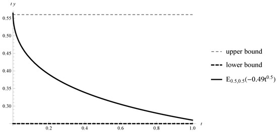
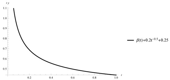
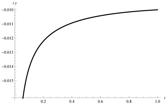
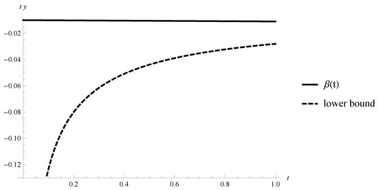
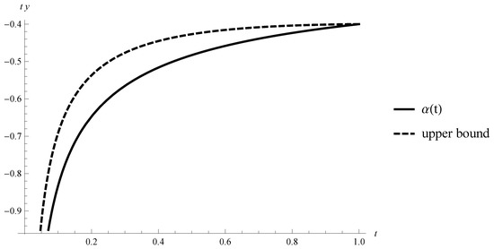
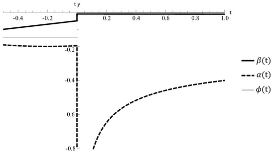
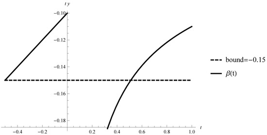
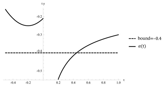
is a mild upper solution of IVP (7) because $\beta \left(t\right)=0.1t-0.05>\varphi \left(t\right)=-0.15$ for $t\in [-0.5,0]$ and $t^{0.5}{(-0.001t-0.01)|}_{t=0}=0>-0.15$. Also, for $t\in (0,1]$ using the inequalities $0.56\ge E_{0.5,0.5}(-0.49{(t-s)}^{0.5})\ge 0.25$ (see the graphs on Figure 1), $\underset{\sigma \in [s-0.5,s]}{sup}\beta \left(\sigma \right)\le -0.01,s\in [0,1]$, $\beta \left(t\right)+0.2t^{-0.5}+0.25>0$ (see the graphs on Figure 2) and $(\beta \left(t\right)+0.2t^{-0.5}+0.25)(-0.0-5)+0.49\beta \left(t\right)<0,t\in [0,1]$ (see the graphs on Figure 3) we obtain the following inequalities (see the graphs on Figure 4)

$$\begin{array}{cc}\hfill \beta \left(t\right)\ge & -0.05\Gamma \left(0.5\right)E_{0.5,0.5}(-0.49t^{0.5})t^{-0.5}\hfill \\ & +0.25{\int }_0^t{(t-s)}^{-0.5}((\beta \left(s\right)+0.2s^{-0.5}+0.25)(-0.0105)+0.49\beta \left(s\right))ds\hfill \\ \hfill \ge & \beta \left(0\right)\Gamma \left(0.5\right)E_{0.5,0.5}(-0.49t^{0.5})t^{-0.5}\hfill \\ & +{\int }_0^t{(t-s)}^{-0.5}{E}_{0.5,0.5}(-0.49{(t-s)}^{0.5})\times \hfill \\ & \times \left(\frac{\beta \left(s\right)+0.2s^{-0.5}+0.25}{s+1}\underset{\sigma \in [s-0.5,s]}{sup}\beta \left(\sigma \right)+0.49\beta \left(s\right)\right)ds.\hfill \end{array}$$

(8)

Figure 1. Graphs of the Mittag–Leffer function and its bounds.

Figure 2. Graph of the function $\beta \left(t\right)+0.2t^{-0.5}+0.25$.

Figure 3. Graph of the function $(\beta \left(t\right)+0.2t^{-0.5}+0.25)(-0.0105)+0.49\beta \left(t\right)$.

Figure 4. Graphs of the function $\beta \left(t\right)$ and its bound in (8).

From Figure 4 it can be seen that inequalities (8) hold for $t\in (0,1]$.

In this case we have $g=\underset{t\in [-0.5,0)}{inf}(0.1t-0.05+0.15)=0.1(-0.5)-0.05+0.15=0.05$.

The function

$$\alpha \left(t\right)=\left\{\begin{array}{cc}0.1{(t+0.2)}^2-0.2,\hfill & t\in [-0.5,0]\hfill \\ -0.2(t^{-0.5}+1),\hfill & t\in (0,1]\hfill \end{array}\right.$$

is a mild lower solution of IVP (7) because $\alpha \left(t\right)=0.1{(t+0.2)}^2-0.2\le 0.1{(-0.5+0.2)}^2-0.2=-0.191<\varphi \left(t\right)=-0.15$ for $t\in [-0.5,0]$ and $t^{0.5}(-0.2t^{-0.5}-0.2){|}_{t=0}=-0.2<-0.15$.

Also, for $t\in (0,1]$ applying the inequalities $\alpha \left(t\right)+0.2t^{-0.5}+0.25=0.05>0,t\in [0,1]$, $\alpha \left(t\right)-0.05=-0.2t^{-0.5}-0.25<0$, and $0>\underset{\sigma \in [s-0.5,s]}{sup}\alpha \left(\sigma \right)\ge \alpha \left(0.5\right)=-0.2{\left(0.5\right)}^{-0.5}-0.2>-0.49$ we get

$$\begin{array}{cc}\hfill \alpha \left(t\right)\le & -0.196\Gamma \left(0.5\right)E_{0.5,0.5}(-0.49t^{0.5})t^{-0.5}\hfill \\ & +0.56\left(0.49\right){\int }_0^t{(t-s)}^{-0.5}(-0.2s^{-0.5}-0.25)ds\hfill \\ \hfill \le & \alpha \left(0\right)\Gamma \left(0.5\right)E_{0.5,0.5}(-0.49t^{0.5})t^{-0.5}\hfill \\ & +{\int }_0^t{(t-s)}^{-0.5}{E}_{0.5,0.5}(-0.49{(t-s)}^{0.5})\times \hfill \\ & \times \left(\frac{\alpha \left(s\right)+0.2t^{-0.5}+0.25}{s+1}\underset{\sigma \in [s-0.5,s]}{sup}\alpha \left(\sigma \right)+0.49\alpha \left(s\right)\right)ds.\hfill \end{array}$$

(9)

From Figure 5 it can be seen that inequalities (9) hold for $t\in (0,1]$.

Figure 5. Graphs of the function $\alpha \left(t\right)$ and its upper bound defined by (9).

In this case $h=\underset{t\in [-0.5,0]}{inf}(-0.15-0.1{(t+0.2)}^2+0.2)=0.041$.

As it can be seen on Figure 6 the inequality $\alpha \left(t\right)\le \beta \left(t\right)$ is valid on $[-0.5,1]$, i.e., the considered mild lower and mild upper solutions of IVP (7) are properly defined.

Figure 6. Graphs of the functions $\beta \left(t\right)$ and $\alpha \left(t\right)$.

To determine the constants M and L in Algorithm I we need to check the conditions for the application of the considered algorithm given in the theoretical Section 5 and Theorem 1. We have $-0.2(t^{-0.5}+1)=\alpha \left(t\right)\le x\le y\le \beta \left(t\right)=-0.1t-0.05\le -0.05$, $-0.49\le \alpha \left(0.5\right)\le \underset{s\in [t-0.5,t]}{sup}\alpha \left(s\right)\le u\le v\le \underset{s\in [t-0.5,t]}{sup}\beta \left(s\right)\le -0.0105$ and therefore, $\frac{y+0.2t^{-0.5}+0.25}{t+1}\ge \frac{-0.2(t^{-0.5}-0.2+0.2t^{-0.5}+0.25}{t+1}=\frac{0.05}{t+1}\ge 0.025$ for $t\in [0,1],x,y,u,v\in \mathbb{R}$ and

$$\begin{array}{cc}\hfill F(t,x,u)-F(t,y,v)& =(x+0.2t^{-0.5}+0.25)\frac{u}{t+1}-(y+0.2t^{-0.5}+0.25)\frac{v}{t+1}\hfill \\ & =\frac{u}{t+1}(x-y)+\frac{y+0.2t^{-0.5}+0.25}{t+1}(u-v)\le -0.49(x-y)+0.025(u-v).\hfill \end{array}$$

Thus, $M=-0.49,L=0.025>0$.

Denote ${\alpha }^{\left(0\right)}\left(t\right)=\alpha \left(t\right)$ and ${\beta }^{\left(0\right)}\left(t\right)=\beta \left(t\right)$ for $t\in [-0.5,1]$.

Based on Step 4 in Algorithm I the n-th lower successive approximation, $n=1,2,\dots$, is defined by

$${\alpha }^{\left(n\right)}\left(t\right)=\left\{\begin{array}{c}-0.15-\frac{0.041}{n},t\in [-0.5,0]\hfill \\ (-0.15-\frac{0.041}{n})\Gamma \left(0.5\right)E_{0.5,0.5}(-0.49t^{0.5})t^{-0.5}\hfill \\ {\displaystyle +{\int }_0^t{(t-s)}^{-0.5}{E}_{0.5,0.5}(-0.49{(t-s)}^{0.5})\times }\hfill \\ {\displaystyle \times \left({\alpha }^{(n-1)}\left(s\right)+0.2s^{-0.5}+0.25\right)\frac{\underset{\sigma \in [s-0.5,s]}{sup}{\alpha }^{(n-1)}\left(\sigma \right)}{s+1}ds}\hfill \\ {\displaystyle -{\int }_0^t{(t-s)}^{-0.5}{E}_{0.5,0.5}(-0.49{(t-s)}^{0.5})\times }\hfill \\ {\displaystyle \times \left(0.49{\alpha }^{(n-1)}\left(s\right)+0.025\left(\underset{\sigma \in [s-0.5,s]}{sup}{\alpha }^{(n-1)}\left(\sigma \right)-\underset{\sigma \in [s-0.5,s]}{sup}{\alpha }^{\left(n\right)}\left(\sigma \right)\right)\right)ds,}\hfill \\ t\in (0,1]\hfill \end{array}\right.$$

(10)

and according to Step 5 in Algorithm I the n-th upper successive approximation, $n=1,2,\dots$, is defined by

$${\beta }^{\left(n\right)}\left(t\right)=\left\{\begin{array}{c}-0.15+\frac{0.05}{n},t\in [-0.5,0]\hfill \\ (-0.15+\frac{0.05}{n})\Gamma \left(0.5\right)E_{0.5,0.5}(-0.49t^{0.5})t^{-0.5}\hfill \\ {\displaystyle +{\int }_0^t{(t-s)}^{-0.5}{E}_{0.5,0.5}(-0.49{(t-s)}^{0.5})\times }\hfill \\ {\displaystyle \left({\beta }^{(n-1)}\left(s\right)+0.2s^{-0.5}+0.25\right)\frac{\underset{\sigma \in [s-0.5,s]}{sup}{\beta }^{(n-1)}\left(\sigma \right)}{s+1}ds}\hfill \\ {\displaystyle -{\int }_0^t{(t-s)}^{-0.5}{E}_{0.5,0.5}(-0.49{(t-s)}^{0.5})\times }\hfill \\ {\displaystyle \times \left(0.49{\beta }^{(n-1)}\left(s\right)+0.025\left(\underset{\sigma \in [s-0.5,s]}{sup}{\beta }^{(n-1)}\left(\sigma \right)-\underset{\sigma \in [s-0.5,s]}{sup}{\beta }^{\left(n\right)}\left(\sigma \right)\right)\right)ds,}\hfill \\ t\in (0,1].\hfill \end{array}\right.$$

Both sequences constructed above converge to the mild solution of IVP (7) (theoretically it follows from Theorem 1).

Now we will illustrate the application of Algorithm II.

Example 2. 

Let $r=0.5,T=1$ and consider the IVP for scalar nonlinear Riemann–Liouville FrDES

$$\begin{array}{c}{}_0^{RL}{D}_t^{0.5}y\left(t\right)=f\left(t\right)\underset{\sigma \in [t-0.5,t]}{sup}y\left(\sigma \right)fort\in (0,1],\hfill \\ y\left(t\right)=-0.155fort\in [-0.5,0],\hfill \\ t^{0.5}{y\left(t\right)|}_{t=0}=-0.155\hfill \end{array}$$

(11)

with $\varphi \left(t\right)=0.5t-0.1,t\in [-0.5,0]$, and $f\left(t\right)=0.2(t+0.2)\in [0.04,0.24]$.

We will introduce two functions and we will prove they are a mild upper solution and a mild lower solution of IVP (11), respectively.

The function $\beta \left(t\right)$ defined by

$$\beta \left(t\right)=\left\{\begin{array}{cc}0.1t-0.1,\hfill & t\in [-0.5,0]\hfill \\ -0.1t^{-0.5}+0.01,\hfill & t\in (0,1]\hfill \end{array}\right.$$

is a mild upper solution of IVP (11) because $\beta \left(t\right)=0.1t-0.1>\varphi \left(t\right)=-0.155$ for $t\in [-0.5,0]$ and $t^{0.5}(-0.1t^{-0.5}+0.01){|}_{t=0}=-0.1>-0.155$. The graph of the function $\beta \left(t\right)$ for $t\in [-0.5,1]$ is shown on Figure 7.

Figure 7. Example 2. Graph of the function $\beta \left(t\right)$.

Additionally, using the inequalities $\underset{\sigma \in [s-0.5,s]}{sup}\beta \left(\sigma \right)\le -0.09<0$ and $0.01\ge -\frac{0.09}{\Gamma (0.5)}{\int }_0^t{(t-s)}^{0.5-1}f\left(s\right)ds$ for $t\in (0,1]$, we get

$$\begin{array}{cc}\hfill \beta \left(t\right)& =-0.1t^{-0.5}+0.01\ge -0.1t^{-0.5}+\frac{1}{\Gamma \left(0.5\right)}{\int }_0^t{(t-s)}^{0.5-1}f\left(s\right)\underset{\sigma \in [s-0.5,s]}{sup}\beta \left(\sigma \right)ds.\hfill \end{array}$$

In this case we have $g=\underset{t\in [-0.5,0)}{inf}(0.1t-0.1+0.155)=0.1(-0.5)-0.1+0.155=0.005$.

The function $\alpha \left(t\right)$ defined by

$$\alpha \left(t\right)=\left\{\begin{array}{cc}{(t+0.2)}^2-0.25,\hfill & t\in [-0.5,0]\hfill \\ -0.2t^{-0.5}-0.1\hfill & t\in (0,1]\hfill \end{array}\right.$$

is a mild lower solution of IVP (11) because $\alpha \left(t\right)={(t+0.2)}^2-0.25<\varphi \left(t\right)=-0.155$ for $t\in [-0.5,0]$ and $t^{0.5}(-0.2t^{-0.5}-0.1){|}_{t=0}=-0.2<-0.155$. The graph of the function $\alpha \left(t\right)$ for $t\in [-0.5,1]$ is given on Figure 8.

Figure 8. Example 2. Graph of the function $\alpha \left(t\right)$.

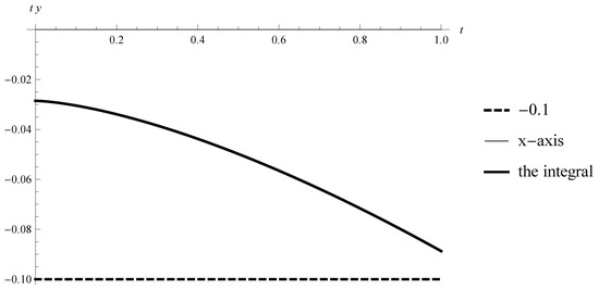
Therefore, for $t\in (0,1]$ applying the inequalities $0\ge \underset{\sigma \in [s-0.5,s]}{sup}\alpha \left(\sigma \right)\ge -0.4$ and $-0.1\le -\frac{0.4}{\Gamma \left(0.5\right)}{\int }_0^t{(t-s)}^{0.5-1}0.2(s+0.2)ds$, and its validity can be seen graphically on Figure 9, we get

$$\begin{array}{cc}\hfill \alpha \left(t\right)& =-0.2t^{-0.5}-0.1\le -0.2t^{-0.5}+\frac{1}{\Gamma \left(0.5\right)}{\int }_0^t{(t-s)}^{0.5-1}0.2(s+0.2)\underset{\sigma \in [s-0.5,s]}{sup}\alpha \left(\sigma \right)ds.\hfill \end{array}$$

Figure 9. Example 2. Graphs of the bound $-0.1$ and the integral.

In this case $h={inf}_{t\in [-0.5,0]}(-0.155-{(t+0.2)}^2)+0.25=(-0.155-{(-0.5+0.2)}^2)+0.25=0.005.$

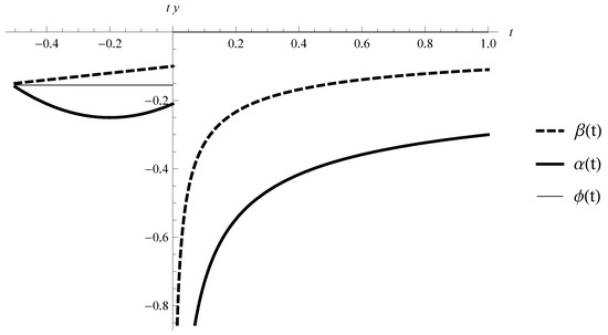
As it can be seen in Figure 10 the inequality $\alpha \left(t\right)\le \beta \left(t\right)$ is valid on $[-0.5,1]$, i.e., the considered lower and upper solutions of IVP (11) are properly defined.

Figure 10. Eaxmple 2. Graphs of the functions $\alpha \left(t\right),\beta \left(t\right),\varphi \left(t\right)$.

To apply the iterative scheme, suggested in Algorithm II we need to check the validity of the corresponding conditions given in the theoretical part in Section 5, Theorem 2. We get

$$\begin{array}{cc}\hfill F(t,u)-F(t,v)& =f\left(t\right)u-f\left(t\right)v=f\left(t\right)(u-v)\le 0.04(u-v)fort\in [0,1],u,v\in \mathbb{R}.\hfill \end{array}$$

Thus $L=0.04>0$ and $\frac{0.04}{\Gamma \left(0.5\right)}=0.56419<1$.

Define the zero approximations ${\alpha }^{\left(0\right)}\left(t\right)=\alpha \left(t\right)$ and ${\beta }^{\left(0\right)}\left(t\right)=\beta \left(t\right)$ for $t\in [-0.5,1]$.

Based on Step $4^{*}$ in Algorithm II the n-th lower successive approximation, $n=1,2,\dots$, is defined by

$${\alpha }^{\left(n\right)}\left(t\right)=\left\{\begin{array}{c}-0.155-\frac{0.005}{n},t\in [-0.5,0]\hfill \\ (-0.155-\frac{0.005}{n})t^{-0.5}\hfill \\ {\displaystyle +\frac{0.2}{\Gamma \left(0.5\right)}{\int }_0^t{(t-s)}^{-0.5}s\underset{\sigma \in [s-0.5,s]}{sup}{\alpha }^{(n-1)}\left(\sigma \right)ds}\hfill \\ {\displaystyle +\frac{0.04}{\Gamma \left(0.5\right)}{\int }_0^t{(t-s)}^{-0.5}\underset{\sigma \in [s-0.5,s]}{sup}{\alpha }^{\left(n\right)}\left(\sigma \right)ds,t\in (0,1],}\hfill \end{array}\right.$$

(12)

and based on Step $5^{*}$ in Algorithm II the n-th lower successive approximation, $n=1,2,\dots$, is given by

$${\beta }^{\left(n\right)}\left(t\right)=\left\{\begin{array}{c}-0.155+\frac{0.095}{n},t\in [-0.5,0]\hfill \\ (-0.155+\frac{0.005}{n})t^{-0.5}\hfill \\ {\displaystyle +\frac{0.2}{\Gamma \left(0.5\right)}{\int }_0^t{(t-s)}^{-0.5}s\underset{\sigma \in [s-0.5,s]}{sup}{\beta }^{(n-1)}\left(\sigma \right)ds}\hfill \\ {\displaystyle +\frac{0.04}{\Gamma \left(0.5\right)}{\int }_0^t{(t-s)}^{-0.5}\underset{\sigma \in [s-0.5,s]}{sup}{\beta }^{\left(n\right)}\left(\sigma \right)ds,t\in (0,1].}\hfill \end{array}\right.$$

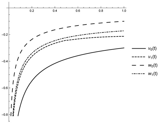
We used CAS Wolfram Mathematica to calculate and graph two successive approximations of mild lower and mild upper solutions (see Figure 11).

Figure 11. Example 2. Graphs of the functions ${\alpha }^i\left(t\right)$ and ${\beta }^i\left(t\right)$, $i=0,1$.

From Figure 11 it can be seen that the suggested iterative scheme in Algorithm II for constructing successive approximations is applicable to the considered IVP (11). As a result we obtain two sequences of successive approximations, which converge uniformly to the mild solution of IVP (11) (for a theoretical proof see Theorem 2).

5. Theoretical Proof of the Algorithms

Now, based on the monotone iterative technique we will suggest an algorithm for approximate solving of FrDES (1), (2). We will prove theoretically the convergence of the suggested sequences of successive approximations. The idea of the formulas for the successive approximations is based on linear RL-fractional differential equations of type (3) and its explicit formula for the solution obtained in [23].

For any two $u,v\in PC\left(\right[-r,T],\mathbb{R})$ and constants $M,\epsilon \in \mathbb{R}$ and $L>0,$ we define the operator $\Omega (u,v,\epsilon ):PC\left(\right[-r,T],\mathbb{R})\times PC\left(\right[-r,T],\mathbb{R})\times \mathbb{R}\to PC\left(\right[-r,T],\mathbb{R})$ by

$$\Omega (u,v,\epsilon )\left(t\right)=\left\{\begin{array}{c}\varphi \left(t\right)+\epsilon ,t\in [-r,0]\hfill \\ (\varphi \left(0\right)+\epsilon )\Gamma \left(q\right)E_{q,q}\left(M{t}^q\right)t^{q-1}\hfill \\ {\displaystyle +{\int }_0^t{(t-s)}^{q-1}{E}_{q,q}\left(M{(t-s)}^q\right)F(s,u\left(s\right),\underset{\sigma \in [s-r,s]}{sup}u\left(\sigma \right))ds}\hfill \\ {\displaystyle -{\int }_0^t{(t-s)}^{q-1}{E}_{q,q}\left(M{(t-s)}^q\right)(Mu\left(s\right)}\hfill \\ {\displaystyle +L(\underset{\sigma \in [s-r,s]}{sup}u\left(\sigma \right)-\underset{\sigma \in [s-r,s]}{sup}v\left(\sigma \right)))ds,t\in (0,T].}\hfill \end{array}\right.$$

Note the particular values of the constants $M,L$ will be defined later. We will prove some properties of the operator $\Omega$.

Lemma 1. 

Let

1. 

The functions $u,\alpha \in PC\left(\right[-r,T],\mathbb{R})$ be such that $u\left(t\right)\le \alpha \left(t\right)$, $t\in [-r,T],$ and $\alpha \left(t\right)=\Omega (u,\alpha ,\epsilon )\left(t\right)$ with $\epsilon \in \mathbb{R}$.

2. 

For any $t\in (0,T]$ the inequality

$$\begin{array}{cc}\hfill & F\left(t,u\left(t\right),\underset{s\in [t-r,t]}{sup}u\left(s\right)\right)-F\left(t,\alpha \left(t\right),\underset{s\in [t-r,t]}{sup}\alpha \left(s\right)\right)\hfill \\ \hfill & \le M\left(u\left(t\right)-\alpha \left(t\right)\right)+L\left(\underset{s\in [t-r,t]}{sup}u\left(s\right)-\underset{s\in [t-r,t]}{sup}\alpha \left(s\right)\right)\hfill \end{array}$$

holds with $M\in \mathbb{R},L>0$.

3. 

The function $\beta \in PC\left(\right[-r,T],\mathbb{R})$ be such that $\beta \left(t\right)=\Omega (v,\beta ,\epsilon +\delta )\left(t\right),t\in [-r,T]$ with $\delta >0$.

Then the inequality $\alpha \left(t\right)<\beta \left(t\right)$ holds for all $t\in [-r,T]$.

Proof. 

Assume the contrary. Since $\alpha \left(t\right)<\beta \left(t\right)$ for $t\in [-r,0]$ and $t^{1-q}\alpha \left(t\right){{|}_{t=0}=\varphi \left(0\right)+\epsilon <\varphi \left(0\right)+\epsilon +\delta =t^{1-q}\beta \left(t\right)|}_{t=0}$ there exists a point $t^{*}\in (0,T]$ such that $\alpha \left(t\right)<\beta \left(t\right)$ for $t\in [-r,t^{*})$ and $\alpha \left(t^{*}\right)=\beta \left(t^{*}\right)$. Then $\underset{\sigma \in [s-r,s]}{sup}\alpha \left(\sigma \right)\le \underset{\sigma \in [s-r,s]}{sup}\beta \left(\sigma \right)$ for $s\in [0,t]$ and

$$\begin{array}{cc}\hfill \alpha \left(t^{*}\right)-\beta \left(t^{*}\right)=& \Omega (u,\alpha ,\epsilon )\left(t^{*}\right)-\Omega (v,\beta ,\epsilon +\delta )\left(t^{*}\right)\hfill \\ \hfill =& -\delta \Gamma \left(q\right)E_{q,q}\left(M{\left(t^{*}\right)}^q\right){\left(t^{*}\right)}^{q-1}\hfill \\ & +L{\int }_0^{t^{*}}{(t^{*}-s)}^{q-1}{E}_{q,q}\left(M{(t^{*}-s)}^q\right)\left(\underset{\sigma \in [s-r,s]}{sup}\alpha \left(\sigma \right)-\underset{\sigma \in [s-r,s]}{sup}\beta \left(\sigma \right)\right)ds\hfill \\ & +{\int }_0^{t^{*}}{(t^{*}-s)}^{q-1}{E}_{q,q}\left(M{(t^{*}-s)}^q\right)\times \hfill \\ & \times \left(F(s,u\left(s\right),\underset{\sigma \in [s-r,s]}{sup}u\left(\sigma \right))-F(s,\alpha \left(s\right),\underset{\sigma \in [s-r,s]}{sup}\alpha \left(\sigma \right))\right)ds\hfill \\ & +{\int }_0^{t^{*}}{(t^{*}-s)}^{q-1}{E}_{q,q}\left(M{(t^{*}-s)}^q\right)\times \hfill \\ & \times \left(M(\alpha \left(s\right)-u\left(s\right))+L(\underset{\sigma \in [s-r,s]}{sup}\alpha \left(\sigma \right)-\underset{\sigma \in [s-r,s]}{sup}u\left(\sigma \right))\right)ds\hfill \\ \hfill \le & -\delta \Gamma \left(q\right)E_{q,q}\left(M{\left(t^{*}\right)}^q\right){\left(t^{*}\right)}^{q-1}\hfill \\ & +{\int }_0^{t^{*}}{(t^{*}-s)}^{q-1}{E}_{q,q}\left(M{(t^{*}-s)}^q\right)\times \hfill \\ & \times \left(M(u\left(s\right)-\alpha \left(s\right))+L(\underset{\sigma \in [s-r,s]}{sup}u\left(\sigma \right)-\underset{\sigma \in [s-r,s]}{sup}\alpha \left(\sigma \right))\right)ds\hfill \\ & +{\int }_0^{t^{*}}{(t^{*}-s)}^{q-1}{E}_{q,q}\left(M{(t^{*}-s)}^q\right)\times \hfill \\ & \times \left(M(\alpha \left(s\right)-u\left(s\right))+L(\underset{\sigma \in [s-r,s]}{sup}\alpha \left(\sigma \right)-\underset{\sigma \in [s-r,s]}{sup}u\left(\sigma \right))\right)ds\hfill \\ \hfill =& -\delta \Gamma \left(q\right)E_{q,q}\left(M{\left(t^{*}\right)}^q\right){\left(t^{*}\right)}^{q-1}<0.\hfill \end{array}$$

The obtained contradiction proves the claim. □

Lemma 2. 

Let

1. 

The functions $u,\alpha \in PC\left(\right[-r,T],\mathbb{R})$ be such that $u\left(t\right)\ge \alpha \left(t\right),t\in [-r,T]$ and $\alpha \left(t\right)=\Omega (u,\alpha ,\epsilon +\delta )\left(t\right)$ with $\epsilon \in \mathbb{R}$, $\delta >0$.

2. 

For any $t\in (0,T]$ the inequality

$$\begin{array}{cc}\hfill & F\left(t,\alpha \left(t\right),\underset{s\in [t-r,t]}{sup}\alpha \left(s\right)\right)-F\left(t,u\left(t\right),\underset{s\in [t-r,t]}{sup}u\left(s\right)\right)\hfill \\ \hfill & \le M(\alpha \left(t\right)-u\left(t\right))+L\left(\underset{s\in [t-r,t]}{sup}\alpha \left(s\right)-\underset{s\in [t-r,t]}{sup}u\left(s\right)\right)\hfill \end{array}$$

holds with $M\in \mathbb{R},L>0$.

3. 

The function $\beta \in PC\left(\right[-r,T],\mathbb{R})$ be such that $\beta \left(t\right)=\Omega (v,\beta ,\epsilon )\left(t\right),t\in [-r,T]$.

Then the inequality $\alpha \left(t\right)>\beta \left(t\right)$ holds for all $t\in [-r,T]$.

Proof. 

The proof is similar to the one in Theorem 1.

Assume the contrary. Since $\alpha \left(t\right)>\beta \left(t\right)$ for $t\in [-r,0]$ and $t^{1-q}\alpha \left(t\right){{|}_{t=0}=\varphi \left(0\right)+\epsilon +\delta >\varphi \left(0\right)+\epsilon =t^{1-q}\beta \left(t\right)|}_{t=0}$ there exists a point $t^{*}\in (0,T]$ such that $\alpha \left(t\right)>\beta \left(t\right)$ for $t\in [-r,t^{*})$ and $\alpha \left(t^{*}\right)=\beta \left(t^{*}\right)$. Then $\underset{\sigma \in [s-r,s]}{sup}\alpha \left(\sigma \right)\ge \underset{\sigma \in [s-r,s]}{sup}\beta \left(\sigma \right)$ for $s\in [0,t]$ and

$$\begin{array}{c}\beta \left(t^{*}\right)-\alpha \left(t^{*}\right)=-\delta \Gamma \left(q\right)E_{q,q}\left(M{\left(t^{*}\right)}^q\right){\left(t^{*}\right)}^{q-1}\hfill \\ -L{\int }_0^{t^{*}}{(t^{*}-s)}^{q-1}{E}_{q,q}\left(M{(t^{*}-s)}^q\right)\left(\underset{\sigma \in [s-r,s]}{sup}\alpha \left(\sigma \right)-\underset{\sigma \in [s-r,s]}{sup}\beta \left(\sigma \right)\right)ds\hfill \\ +{\int }_0^{t^{*}}{(t^{*}-s)}^{q-1}{E}_{q,q}\left(M{(t^{*}-s)}^q\right)\left(F(s,\alpha \left(s\right),\underset{\sigma \in [s-r,s]}{sup}\alpha \left(\sigma \right))-F(s,u\left(s\right),\underset{\sigma \in [s-r,s]}{sup}u\left(\sigma \right))\right)ds\hfill \\ -{\int }_0^{t^{*}}{(t^{*}-s)}^{q-1}{E}_{q,q}\left(M{(t^{*}-s)}^q\right)\left(M(\alpha \left(s\right)-u\left(s\right))+L(\underset{\sigma \in [s-r,s]}{sup}\alpha \left(\sigma \right)-\underset{\sigma \in [s-r,s]}{sup}u\left(\sigma \right))\right)ds\hfill \\ \le -\delta \Gamma \left(q\right)E_{q,q}\left(M{\left(t^{*}\right)}^q\right){\left(t^{*}\right)}^{q-1}\hfill \\ +{\int }_0^{t^{*}}{(t^{*}-s)}^{q-1}{E}_{q,q}\left(M{(t^{*}-s)}^q\right)\left(M(\alpha \left(s\right)-u\left(s\right))+L(\underset{\sigma \in [s-r,s]}{sup}\alpha \left(\sigma \right)-\underset{\sigma \in [s-r,s]}{sup}u\left(\sigma \right))\right)ds\hfill \\ -{\int }_0^{t^{*}}{(t^{*}-s)}^{q-1}{E}_{q,q}\left(M{(t^{*}-s)}^q\right)\left(M(\alpha \left(s\right)-u\left(s\right))+L(\underset{\sigma \in [s-r,s]}{sup}\alpha \left(\sigma \right)-\underset{\sigma \in [s-r,s]}{sup}u\left(\sigma \right))\right)ds\hfill \\ =-\delta \Gamma \left(q\right)E_{q,q}\left(M{\left(t^{*}\right)}^q\right){\left(t^{*}\right)}^{q-1}<0.\hfill \end{array}$$

The obtained contradiction proves the claim. □

Now we will prove the convergence.

Theorem 1. 

Let the following conditions be fulfilled:

1. 

Let the functions $\alpha ,\beta \in PC([-r,T],\mathbb{R})\cup C_{1-q}\left([0,T]\right)$ be a mild lower solution and a mild upper solution of the IVP for FrDES (1), respectively, defined by Definition 3 with $\mu =M$ such that $\alpha \left(t\right)\le \beta \left(t\right)$ for $t\in [0,T]$ and

$$\begin{array}{c}\varphi \left(0\right)-\alpha \left(0\right)>\underset{t\in [-r,0]}{inf}(\varphi \left(t\right)-\alpha \left(t\right))=h>0,\hfill \\ \beta \left(0\right)-\varphi \left(0\right)>\underset{t\in [-r,0]}{inf}(\beta \left(t\right)-\varphi \left(t\right))=g>0.\hfill \end{array}$$

(13)

2. 

The function $F\in C\left(\right[0,T]\times \mathbb{R}\times \mathbb{R},\mathbb{R})$ and there exist constants $M\in \mathbb{R}$ and $L>0$ such that for any $t\in [0,T]$, $x,y,u,v\in \mathbb{R}:\alpha \left(t\right)\le x\le y\le \beta \left(t\right)$, $\underset{\sigma \in [t-r,t]}{sup}\alpha \left(\sigma \right)\le u\le v\le \underset{\sigma \in [t-r,t]}{sup}\beta \left(\sigma \right)$ the inequality $F(t,x,u)-F(t,y,v)\le M(x-y)+L(u-v)$ holds.

Then there exists two sequences of functions ${\left\{{\alpha }^{\left(n\right)}\left(t\right)\right\}}_0^{\infty }$ and ${\left\{{\beta }^{\left(n\right)}\left(t\right)\right\}}_0^{\infty }$, $t\in [-r,T]$, such that:

a. 

The sequences $\left\{{\alpha }^{\left(n\right)}\left(t\right)\right\}$ and $\left\{{\beta }^{\left(n\right)}\left(t\right)\right\}$ are defined by ${\alpha }^{\left(0\right)}\left(t\right)=\alpha \left(t\right),{\beta }^{\left(0\right)}\left(t\right)=\beta \left(t\right)$ and

$${\alpha }^{\left(n\right)}\left(t\right)=\Omega \left({\alpha }^{(n-1)},{\alpha }^{\left(n\right)},-\frac{h}{n}\right)\left(t\right),{\beta }^{\left(n\right)}\left(t\right)=\Omega \left({\beta }^{(n-1)},{\beta }^{\left(n\right)},\frac{g}{n}\right)\left(t\right)forn\ge 1,$$

where the constants $M,L$ are defined in condition 2.

b. 

The sequence ${\left\{{\alpha }^{\left(j\right)}\left(t\right)\right\}}_{j=0}^{\infty }$ is increasing, i.e., ${\alpha }^{(j-1)}\left(t\right)\le {\alpha }^{\left(j\right)}\left(t\right)$ for $t\in [-r,T]$ and $t^{1-q}{\alpha }^{(j-1)}\left(t\right){{|}_{t=0}\le t^{1-q}{\alpha }^{\left(j\right)}\left(t\right)|}_{t=0}$, $j=1,2,\dots$.

c. 

The sequence ${\left\{{\beta }^{\left(j\right)}\left(t\right)\right\}}_{j=0}^{\infty }$ is decreasing, i.e., ${\beta }^{(j-1)}\left(t\right)\ge {\beta }^{\left(j\right)}\left(t\right)$ for $t\in (0,T]$ and $t^{1-q}{\beta }^{\left(j\right)}\left(t\right){{|}_{t=0}\le t^{1-q}{\beta }^{(j-1)}\left(t\right)|}_{t=0}$, $j=1,2,\dots$.

d. 

The inequalities

$${\alpha }^{\left(k\right)}\left(t\right)\le {\beta }^{\left(k\right)}\left(t\right)fort\in [-r,T],and{t}^{1-q}{\alpha }^{\left(k\right)}\left(t\right){{|}_{t=0}\le t^{1-q}{\beta }^{\left(k\right)}\left(t\right)|}_{t=0},k=1,2,\dots$$

(14)

hold.

e. 

$\underset{k\to \infty }{lim}{\alpha }^{\left(n\right)}\left(t\right)=\underset{k\to \infty }{lim}{\beta }^{\left(n\right)}\left(t\right)=\varphi \left(t\right)$ uniformly on $[0,T]$.

f. 

The sequences ${\left\{t^{1-q}{\alpha }^{\left(n\right)}\left(t\right)\right\}}_0^{\infty }$ and ${\left\{t^{1-q}{\beta }^{\left(n\right)}\left(t\right)\right\}}_0^{\infty }$ converge uniformly on the interval $[0,T]$ and let $\tilde{V}\left(t\right)=\underset{k\to \infty }{lim}{t}^{1-q}{\alpha }^{\left(n\right)}\left(t\right)$, $\tilde{W}\left(t\right)=\underset{k\to \infty }{lim}{t}^{1-q}{\beta }^{\left(n\right)}\left(t\right)$ on $[0,T]$.

g. 

The inequalities ${\alpha }^{\left(n\right)}\left(t\right)\le V\left(t\right)\le W\left(t\right)\le {\beta }^{\left(n\right)}\left(t\right)$ hold on $[0,T]$ for any $n=0,1,2,\dots$ where

$$V\left(t\right)=\left\{\begin{array}{cc}\varphi \left(t\right),\hfill & t\in [-r,0]\hfill \\ t^{q-1}\tilde{V}\left(t\right)\hfill & t\in (0,T],\hfill \end{array}\right.W\left(t\right)=\left\{\begin{array}{cc}\varphi \left(t\right),\hfill & t\in [-r,0]\hfill \\ t^{q-1}\tilde{W}\left(t\right)\hfill & t\in (0,T].\hfill \end{array}\right.$$

h. 

The functions $V\left(t\right)$ and $W\left(t\right)$ are mild solutions of the IVP for FrDES (1), (2) on $[-r,T]$.

Proof. 

Let ${\alpha }^{\left(0\right)}\left(t\right)=\alpha \left(t\right)$, ${\beta }^{\left(0\right)}\left(t\right)=\beta \left(t\right)$ for $t\in [-r,T]$ and ${\alpha }^{\left(n\right)}\left(t\right)=\Omega \left({\alpha }^{(n-1)},{\alpha }^{\left(n\right)},-\frac{h}{n}\right)\left(t\right)$, ${\beta }^{\left(n\right)}\left(t\right)=\Omega \left({\beta }^{(n-1)},{\beta }^{\left(n\right)},\frac{g}{n}\right)\left(t\right)$, $n=1,2,3,\dots$.

We will prove the inequality

$${\alpha }^{\left(0\right)}\left(t\right)\le {\alpha }^{\left(1\right)}\left(t\right),t\in [-r,T].$$

(15)

For $t\in [-r,0]$ from Definition 3 and the definition of the constant h we get ${\alpha }^{\left(1\right)}\left(t\right)=\varphi \left(t\right)-h\ge \varphi \left(t\right)-(\varphi \left(t\right)-{\alpha }^{\left(0\right)}\left(t\right))={\alpha }^{\left(0\right)}\left(t\right),t\in [-r,0]$.

Also, from Condition 1 ${\alpha }^{\left(0\right)}\left(0\right)<\varphi \left(0\right)-h={\alpha }^{\left(1\right)}\left(0\right)$.

Assume there exists a point $t^{*}\in (0,T]$ such that ${\alpha }^{\left(0\right)}\left(t\right)<{\alpha }^{\left(1\right)}\left(t\right),t\in [0,t^{*})$ and ${\alpha }^{\left(0\right)}\left(t^{*}\right)={\alpha }^{\left(1\right)}\left(t^{*}\right).$ Then from Condition 1, Definition 3, and the inequality $\alpha \left(0\right)=\varphi \left(0\right)-\left(\varphi \right(0)-\alpha (0\left)\right)<\varphi \left(0\right)-h$ the inequality

$$\begin{array}{cc}\hfill {\alpha }^{\left(0\right)}\left(t^{*}\right)& \le \alpha \left(0\right)\Gamma \left(q\right)E_{q,q}\left(M{\left(t^{*}\right)}^q\right){\left(t^{*}\right)}^{q-1}\hfill \\ & +{\int }_0^{t^{*}}{(t^{*}-s)}^{q-1}{E}_{q,q}\left(M{(t^{*}-s)}^q\right)F(s,{\alpha }^{\left(0\right)}\left(s\right),\underset{\sigma \in [s-r,s]}{sup}{\alpha }^{\left(0\right)}\left(\sigma \right)ds\hfill \\ & -{\int }_0^{t^{*}}{(t^{*}-s)}^{q-1}{E}_{q,q}\left(M{(t^{*}-s)}^q\right)M{\alpha }^{\left(0\right)}\left(t\right)ds\hfill \\ & <(\varphi \left(0\right)-h)\Gamma \left(q\right)E_{q,q}\left(M{\left(t^{*}\right)}^q\right){\left(t^{*}\right)}^{q-1}\hfill \\ & +{\int }_0^{t^{*}}{(t^{*}-s)}^{q-1}{E}_{q,q}\left(M{(t^{*}-s)}^q\right)F(s,{\alpha }^{\left(0\right)}\left(s\right),\underset{\sigma \in [s-r,s]}{sup}{\alpha }^{\left(0\right)}\left(\sigma \right))ds\hfill \\ & -{\int }_0^{t^{*}}{(t-s)}^{q-1}{E}_{q,q}\left(M{(t^{*}-s)}^q\right)\times \hfill \\ & \times \left(M{\alpha }^{\left(0\right)}\left(t\right)+L\left(\underset{\sigma \in [s-r,s]}{sup}{\alpha }^{\left(0\right)}\left(\sigma \right)-\underset{\sigma \in [s-r,s]}{sup}{\alpha }^{\left(1\right)}\left(\sigma \right)\right)\right)ds\hfill \\ & =\Omega ({\alpha }^{\left(0\right)},{\alpha }^{\left(1\right)},-h)\left(t^{*}\right)={\alpha }^{\left(1\right)}\left(t^{*}\right)\hfill \end{array}$$

holds. The obtained contradiction proves the inequality (15) on $(0,T]$.

We will prove the inequality

$${\beta }^{\left(0\right)}\left(t\right)\ge {\beta }^{\left(1\right)}\left(t\right),t\in [-r,T].$$

(16)

For $t\in [-r,0]$ from Definition 3 and the definition of the constant g we get ${\beta }^{\left(1\right)}\left(t\right)=\varphi \left(t\right)+g\le \varphi \left(t\right)+(\beta \left(t\right)-\varphi \left(t\right))={\beta }^{\left(0\right)}\left(t\right),t\in [-r,0]$.

Also, from Condition 1 ${\beta }^{\left(0\right)}\left(0\right)>\varphi \left(0\right)+g={\beta }^{\left(1\right)}\left(0\right)$.

Assume there exists a point $t^{*}\in (0,T]$ such that ${\beta }^{\left(0\right)}\left(t\right)>{\beta }^{\left(1\right)}\left(t\right),t\in [0,t^{*})$ and ${\beta }^{\left(0\right)}\left(t^{*}\right)={\beta }^{\left(1\right)}\left(t^{*}\right).$ Then from Condition 1, Definition 3, and the inequalities $\beta \left(0\right)=\varphi \left(0\right)+\left(\beta \right(0)-\varphi (0\left)\right)>\varphi \left(0\right)+g$ and $\underset{\sigma \in [s-r,s]}{sup}{\beta }^{\left(0\right)}\left(\sigma \right)-\underset{\sigma \in [s-r,s]}{sup}{\beta }^{\left(1\right)}\left(\sigma \right)\ge 0,s\in [0,t^{*}]$ we obtain

$$\begin{array}{cc}\hfill {\beta }^{\left(1\right)}\left(t\right)& =\Omega ({\beta }^{\left(0\right)},{\beta }^{\left(1\right)},g)\left(t\right)=(\varphi \left(0\right)+g)\Gamma \left(q\right)E_{q,q}\left(M{t}^q\right)t^{q-1}\hfill \\ & +{\int }_0^t{(t-s)}^{q-1}{E}_{q,q}\left(M{(t-s)}^q\right)F(s,{\beta }^{\left(0\right)}\left(s\right),\underset{\sigma \in [s-r,s]}{sup}{\beta }^{\left(0\right)}\left(\sigma \right))ds\hfill \\ & -{\int }_0^t{(t-s)}^{q-1}{E}_{q,q}\left(M{(t-s)}^q\right)\times \hfill \\ & \times \left(M{\beta }^{\left(0\right)}\left(t\right)+L\left(\underset{\sigma \in [s-r,s]}{sup}{\beta }^{\left(0\right)}\left(\sigma \right)-\underset{\sigma \in [s-r,s]}{sup}{\beta }^{\left(1\right)}\left(\sigma \right)\right)\right)ds\hfill \\ & <\beta \left(0\right)\Gamma \left(q\right)E_{q,q}\left(M{t}^q\right)t^{q-1}\hfill \\ & +{\int }_0^t{(t-s)}^{q-1}{E}_{q,q}\left(M{(t-s)}^q\right)F(s,{\beta }^{\left(0\right)}\left(s\right),\underset{\sigma \in [s-r,s]}{sup}{\beta }^{\left(0\right)}\left(\sigma \right))ds\hfill \\ & -{\int }_0^t{(t-s)}^{q-1}{E}_{q,q}\left(M{(t-s)}^q\right)M{\beta }^{\left(0\right)}\left(t\right)ds\le {\beta }^{\left(0\right)}\left(t^{*}\right)\hfill \end{array}$$

holds. The contradiction proves the inequality (16).

We use induction to prove properties of the sequences of successive approximations.

Assume that for a natural number $n\ge 2$ the inequality ${\alpha }^{(n-2)}\left(t\right)\le {\alpha }^{(n-1)}\left(t\right)$, $t\in [-r,T]$ holds. We will prove that ${\alpha }^{(n-1)}\left(t\right)\le {\alpha }^{\left(n\right)}\left(t\right)$, $t\in [-r,T]$.

For $t\in [-r,0]$ we get ${\alpha }^{\left(n\right)}\left(t\right)=\varphi \left(t\right)-\frac{h}{n}=\varphi \left(t\right)-\frac{h}{n-1}-\frac{h}{n}+\frac{h}{n-1}={\alpha }^{(n-1)}\left(t\right)+\frac{h}{n(n-1)}$.

Therefore, for the functions $u\equiv {\alpha }^{(n-2)},\alpha \equiv {\alpha }^{(n-1)},\beta \equiv {\alpha }^{\left(n\right)}$ and the constants $\delta =\frac{h}{n(n-1)}>0$ and $\epsilon =-\frac{h}{n-1}$ according to Lemma 1 we have from the assumption $u\left(t\right)\le \alpha \left(t\right),t\in [-r,T]$ and $\alpha \left(t\right)=\Omega (u,\alpha ,\epsilon )\left(t\right)$ and $\beta \left(t\right)=\Omega (\alpha ,\beta ,\epsilon +\delta )$ the inequality $\alpha \left(t\right)={\alpha }^{(n-1)}\left(t\right)<\beta \left(t\right)={\alpha }^{\left(n\right)}\left(t\right)$ holds for all $t\in [-r,T]$.

Similarly, applying Lemma 2 instead of Lemma 1 we can prove

$${\beta }^{\left(n\right)}\left(t\right)\ge {\beta }^{(n+1)}\left(t\right),fort\in [-r,T],n=1,2,\dots .$$

Using induction we will prove that for any natural number n the inequality

$${\alpha }^{\left(n\right)}\left(t\right)\le {\beta }^{\left(n\right)}\left(t\right),t\in [-r,T]$$

(17)

holds.

Assume the inequality ${\alpha }^{(n-1)}\left(t\right)\le {\beta }^{(n-1)}\left(t\right),t\in [-r,T],$ holds.

For $t\in [-r,0]$ we have ${\alpha }^{\left(n\right)}\left(t\right)=\varphi \left(t\right)-\frac{h}{n}<\varphi \left(t\right)<\varphi \left(t\right)+\frac{g}{n}={\beta }^{\left(n\right)}\left(t\right)$, i.e., (17) holds. Assume there exists a point $t^{*}\in (0,T]$ such that ${\alpha }^{\left(n\right)}\left(t\right)<{\beta }^{\left(n\right)}\left(t\right),t\in [0,t^{*})$ and ${\alpha }^{\left(n\right)}\left(t^{*}\right)={\beta }^{\left(n\right)}\left(t^{*}\right).$ Then we get the inequality

$$\begin{array}{c}0={\alpha }^{\left(n\right)}\left(t^{*}\right)-{\beta }^{\left(n\right)}\left(t^{*}\right)=-\frac{h+g}{n}\Gamma \left(q\right)E_{q,q}\left(M{t^{*}}^q\right){\left(t^{*}\right)}^{q-1}\hfill \\ +{\int }_0^{t^{*}}{(t^{*}-s)}^{q-1}{E}_{q,q}\left(M{(t^{*}-s)}^q\right)F(s,{\alpha }^{(n-1)}\left(s\right),\underset{\sigma \in [s-r,s]}{sup}{\alpha }^{(n-1)}\left(\sigma \right))ds\hfill \\ -{\int }_0^{t^{*}}{(t^{*}-s)}^{q-1}{E}_{q,q}\left(M{(t^{*}-s)}^q\right)F(s,{\beta }^{(n-1)}\left(s\right),\underset{\sigma \in [s-r,s]}{sup}{\beta }^{(n-1)}\left(\sigma \right))ds\hfill \\ -{\int }_0^{t^{*}}{(t^{*}-s)}^{q-1}{E}_{q,q}\left(M{(t^{*}-s)}^q\right)\times \hfill \\ \times \left(M{\alpha }^{(n-1)}\left(s\right)+L(\underset{\sigma \in [s-r,s]}{sup}{\alpha }^{(n-1)}\left(\sigma \right)-\underset{\sigma \in [s-r,s]}{sup}{\alpha }^{\left(n\right)}\left(\sigma \right))\right))ds\hfill \\ +{\int }_0^{t^{*}}{(t^{*}-s)}^{q-1}{E}_{q,q}\left(M{(t^{*}-s)}^q\right)\times \hfill \\ \times \left(M{\beta }^{(n-1)}\left(s\right)+L(\underset{\sigma \in [s-r,s]}{sup}{\beta }^{(n-1)}\left(\sigma \right)-\underset{\sigma \in [s-r,s]}{sup}{\beta }^{\left(n\right)}\left(\sigma \right))\right))ds\hfill \\ <{\int }_0^{t^{*}}{(t^{*}-s)}^{q-1}{E}_{q,q}\left(M{(t-s)}^q\right)L\left(\underset{\sigma \in [s-r,s]}{sup}{\alpha }^{\left(n\right)}\left(\sigma \right)-\underset{\sigma \in [s-r,s]}{sup}{\beta }^{\left(n\right)}\left(\sigma \right)\right)ds\le 0.\hfill \end{array}$$

The obtained contradiction proves the inequality (17) and the claim (d).

The claim (e) follows from the definition of the functions ${\alpha }^{\left(n\right)}\left(t\right)$ and ${\beta }^{\left(n\right)}\left(t\right)$ for $t\in [-r,0]$.

Now consider the sequences ${\{{\tilde{\alpha }}^{\left(n\right)}\left(t\right)\}}_0^{\infty }$ and ${\{{\tilde{\beta }}^{\left(n\right)}\left(t\right)\}}_0^{\infty }$ for $t\in [0,T]$ defined by ${\tilde{\alpha }}^{\left(n\right)}\left(t\right)=t^{1-q}(\varphi \left(t\right)-\frac{h}{n})$, ${\tilde{\beta }}^{\left(n\right)}\left(t\right)=t^{1-q}(\varphi \left(t\right)+\frac{g}{n})$ for $t\in [-r,0]$ and

$$\begin{array}{cc}\hfill {\tilde{\alpha }}^{\left(n\right)}\left(t\right)& =t^{1-q}{\alpha }^{\left(n\right)}\left(t\right)=\left(\varphi \left(0\right)-\frac{h}{n}\right)\Gamma \left(q\right)E_{q,q}\left(M{t}^q\right)\hfill \\ & +t^{1-q}{\int }_0^t{(t-s)}^{q-1}{E}_{q,q}\left(M{(t-s)}^q\right)F(s,{\alpha }^{(n-1)}\left(s\right),\underset{\sigma \in [s-r,s]}{sup}{\alpha }^{(n-1)}\left(\sigma \right))ds\hfill \\ & -{\int }_0^t{(t-s)}^{q-1}{E}_{q,q}\left(M{(t-s)}^q\right)(M{\alpha }^{(n-1)}\left(s\right)\hfill \\ & +L(\underset{\sigma \in [s-r,s]}{sup}{\alpha }^{(n-1)}\left(\sigma \right)-\underset{\sigma \in [s-r,s]}{sup}{\alpha }^{\left(n\right)}\left(\sigma \right)))ds\hfill \\ & =\left(\varphi \left(0\right)-\frac{h}{n}\right)\Gamma \left(q\right)E_{q,q}\left(M{t}^q\right)\hfill \\ & +t^{1-q}{\int }_0^t{(t-s)}^{q-1}{E}_{q,q}\left(M{(t-s)}^q\right)F(s,s^{q-1}{\tilde{\alpha }}^{(n-1)}\left(s\right),\underset{\sigma \in [s-r,s]}{sup}{s}^{q-1}{\tilde{\alpha }}^{(n-1)}\left(\sigma \right))ds\hfill \\ & -{\int }_0^t{(t-s)}^{q-1}{E}_{q,q}\left(M{(t-s)}^q\right)(M{s}^{q-1}{\tilde{\alpha }}^{(n-1)}\left(s\right)\hfill \\ & +L(\underset{\sigma \in [s-r,s]}{sup}{\sigma }^{q-1}{\tilde{\alpha }}^{(n-1)}\left(\sigma \right)-\underset{\sigma \in [s-r,s]}{sup}{\sigma }^{q-1}{\tilde{\alpha }}^{\left(n\right)}\left(\sigma \right)))ds,t\in [0,T]\hfill \end{array}$$

(18)

and

$$\begin{array}{cc}\hfill {\tilde{\beta }}^{\left(n\right)}\left(t\right)& =t^{1-q}{\beta }^{\left(n\right)}\left(t\right)=\left(\varphi \left(0\right)+\frac{g}{n}\right)\Gamma \left(q\right)E_{q,q}\left(M{t}^q\right)\hfill \\ & +t^{1-q}{\int }_0^t{(t-s)}^{q-1}{E}_{q,q}\left(M{(t-s)}^q\right)F(t,{\beta }^{(n-1)}\left(s\right),\underset{\sigma \in [s-r,s]}{sup}{\beta }^{(n-1)}\left(\sigma \right))ds\hfill \\ & -{\int }_0^t{(t-s)}^{q-1}{E}_{q,q}\left(M{(t-s)}^q\right)(M{\beta }^{(n-1)}\left(s\right)\hfill \\ & +L(\underset{\sigma \in [s-r,s]}{sup}{\beta }^{(n-1)}\left(\sigma \right)-\underset{\sigma \in [s-r,s]}{sup}{\beta }^{\left(n\right)}\left(\sigma \right)))ds,t\in [0,T].\hfill \end{array}$$

(19)

Both sequences are increasing and decreasing, respectively, and bounded. Therefore, they are uniformly convergent on $[0,T]$. Denote, $\tilde{V}\left(t\right)=\underset{n\to \infty }{lim}{\tilde{\alpha }}^{\left(n\right)}\left(t\right)$ and $\tilde{W}\left(t\right)=\underset{n\to \infty }{lim}{\tilde{\beta }}^{\left(n\right)}\left(t\right),t\in [0,T].$ According to the above proved claims (b), (c) and (d) the inequalities

$$\begin{array}{c}{\tilde{\alpha }}^{\left(n\right)}\left(t\right)\le \tilde{V}\left(t\right),t\in [0,T],\tilde{W}\left(t\right)\le {\tilde{\beta }}^{\left(n\right)}\left(t\right),t\in [0,T],n=0,1,2,\dots ,\hfill \\ \tilde{V}\left(t\right)\le \tilde{W}\left(t\right),t\in [0,T]\hfill \end{array}$$

(20)

hold. Therefore, the claim (f) is proved.

For any $t\in [0,T]$ we have $\underset{n\to \infty }{lim}{t}^{q-1}{\tilde{\alpha }}^{\left(n\right)}\left(t\right)=V\left(t\right)$ and $\underset{n\to \infty }{lim}{t}^{q-1}{\tilde{\alpha }}^{\left(n\right)}\left(t\right)=\varphi \left(t\right)=V\left(t\right)$ for $t\in [-r,0]$. Therefore, $\underset{n\to \infty }{lim}\underset{s\in [t-r,t]}{sup}{s}^{q-1}{\tilde{\alpha }}^{\left(n\right)}\left(s\right)=\underset{s\in [t-r,t]}{sup}V\left(t\right)$.

For any point $t\in (0,T]$ we take the limit in (18) and obtain the Volterra fractional integral equation

$$\begin{array}{cc}\hfill V\left(t\right)& =\varphi \left(0\right)\Gamma \left(q\right)E_{q,q}\left(M{t}^q\right)t^{1-q}\hfill \\ & +{\int }_0^t{(t-s)}^{q-1}{E}_{q,q}\left(M{(t-s)}^q\right)\times \hfill \\ & \times \left(F(s,V\left(s\right),\underset{\sigma \in [s-r,s]}{sup}V\left(\sigma \right))-MV\left(s\right)\right)ds,fort\in (0,T].\hfill \end{array}$$

Therefore, the function $V\left(t\right)$ is a mild solution of (1), (2).

Similar is the proof about $W\left(t\right)$.

Proof of claim (g). From claim (d) and the inequality (14) it follows that $t^{1-q}{\alpha }^{\left(k\right)}\left(t\right)\le t^{1-q}{\beta }^{\left(k\right)}\left(t\right)$ for any fixed $t\in (0,T]$ and $k=1,2,\dots$. Then applying claim (e) we get $t^{1-q}{\alpha }^{\left(k\right)}\left(t\right)\le t^{1-q}V\left(t\right)\le t^{1-q}W\left(t\right)\le t^{1-q}{\beta }^{\left(k\right)}\left(t\right)$ for any fixed $t\in (0,T]$. Therefore, ${\alpha }^{\left(k\right)}\left(t\right)\le V\left(t\right)\le W\left(t\right)\le {\beta }^{\left(k\right)}\left(t\right)$ for any on $t\in (0,T]$. □

In the special case when the right hand side part of the Equations (1), (2) does not depend on the current state of the unknown function we use the following operator $\Lambda (v,\epsilon ):PC\left(\right[-r,T]\times PC([-r,T],\mathbb{R}),\mathbb{R})\times (0,\infty )\to PC\left(\right[-r,T],\mathbb{R})$

$$\Lambda (u,v,\epsilon )\left(t\right)=\{\begin{array}{c}\varphi \left(t\right)+\epsilon ,t\in [-r,0]\hfill \\ (\varphi \left(0\right)+\epsilon )t^{q-1}\hfill \\ +\frac{1}{\Gamma \left(q\right)}{\int }_0^t{(t-s)}^{q-1}F(s,\underset{\sigma \in [s-r,s]}{sup}u\left(\sigma \right))ds\hfill \\ -\frac{L}{\Gamma \left(q\right)}{\int }_0^t{(t-s)}^{q-1}\left(\underset{\sigma \in [s-r,s]}{sup}u\left(\sigma \right)-\underset{\sigma \in [s-r,s]}{sup}v\left(\sigma \right)\right)ds,t\in (0,T]\hfill \end{array}$$

to obtain the following easier iterative scheme:

Theorem 2. 

Let the condition 1 of Theorem 1 be satisfied and the function $F\in C\left(\right[0,T]\times \mathbb{R},\mathbb{R})$ and there exist a constant $L>0$ such that for any $t\in [0,T],u,v\in \mathbb{R}:$$\underset{\sigma \in [t-r,t]}{sup}\alpha \left(\sigma \right)\le u\le v\le \underset{\sigma \in [t-r,t]}{sup}\beta \left(\sigma \right)$ the inequality $F(t,u)-F(t,v)\le L(u-v)$ holds.

Then the claims of Theorem 1 are true with replacing the operator Ω by Λ.

6. Conclusions

A scalar nonlinear Riemann–Liouville fractional differential equation with a special type of delay is investigated. The delay is defined by the supremum of the unknown function on a finite past time interval. The presence of the supremum in the equation, additionally to the fractional derivative, leads to decreasing the set of equations with explicit solutions. It requires the application of approximate methods. In this paper, an iterative scheme, giving an asymptotic solution as a limit of two sequences, is suggested. This scheme is based on the so-called monotone iterative technique. Initially, a mild lower solution and a mild upper solution of the studied problem are defined and applied as initial approximations of the unknown solution. Two algorithms for the construction of two sequences of successive approximations are provided and their monotone convergence from above and from below to a mild solution of the given problem is proved. The practical applications of both algorithms are illustrated by examples. Note, since the studied problem is still new and not solved well, the question about the existence and uniqueness is an open question and it is a subject for investigation in a future theoretical paper.

References

- Das, S. Functional Fractional Calculus; Springer: Berlin, Germany, 2011. [Google Scholar]
- Podlubny, I. Fractional Differential Equations; Academic Press: Cambridge, MA, USA, 1999. [Google Scholar]
- Wang, S.; He, S.; Yousefpour, A.; Jahanshahi, H.; Repnik, R.; Perc, M. Chaos and complexity in a fractional-order financial system with time delays. Chaos Soliton Fract. 2020, 131, 109521. [Google Scholar] [CrossRef]
- Wang, S.; Bekiros, S.; Yousefpour, A.; He, S.; Castillo, O.; Jahanshahi, H. Synchronization of fractional time-delayed financial system using a novel type-2 fuzzy active control method. Chaos Soliton Fract. 2020, 136, 109768. [Google Scholar] [CrossRef]
- Hageman, L.A.; Young, D.M. Applied Iterative Methods; Dover Publications: North Chelmsford, MA, USA, 2012. [Google Scholar]
- Argyros, I.K.; Regmi, S. Undergraduate Research at Cameron University on Iterative Procedures in Banach and Other Spaces; Nova Science Publisher: New York, NY, USA, 2019. [Google Scholar]
- Agarwal, R.; Golev, A.; Hristova, S.; O’Regan, D. Iterative techniques with computer realization for initial value problems for Riemann–Liouville fractional differential equations. J. Appl. Anal. 2020, 26, 21–47. [Google Scholar] [CrossRef]
- Agarwal, R.; Hristova, S.; Golev, A.; Stefanova, K. Monotone-iterative method for mixed boundary value problems for generalized difference equations with “maxima”. J. Appl. Math. Comput. 2013, 43, 213–233. [Google Scholar] [CrossRef]
- Agarwal, R.; Golev, A.; Hristova, S.; O’Regan, D.; Stefanova, K. Iterative techniques with computer realization for the initial value problem for Caputo fractional differential equations. J. Appl. Math. Comput. 2017, 58, 433–467. [Google Scholar] [CrossRef]
- Bai, Z.; Zhang, S.; Sun, S.; Yin, C. Monotone iterative method for fractional differential equations. Electron. J. Differ. Equ. 2016, 6, 1–8. [Google Scholar]
- Deekshitulu, G. Generalized monotone iterative technique for fractional R-L differential equations. Nonlinear Stud. 2009, 16, 85–94. [Google Scholar]
- Denton, Z. Monotone method for Riemann-Liouville multi-order fractional differential systems. Opusc. Math. 2016, 36, 189–206. [Google Scholar] [CrossRef]
- Denton, Z.; Ng, P.W.; Vatsala, A.S. Quasilinearization method via lower and upper solutions for Riemann-Liouville fractional differential equations. Nonlinear Dyn. Syst. Theory 2011, 11, 239–251. [Google Scholar]
- Hristova, S.; Golev, A.; Stefanova, K. Approximate method for boundary value problems of anti-periodic type for differential equations with “maxima”. Bound. Value Probl. 2013, 1, 12. [Google Scholar] [CrossRef][Green Version]
- Ladde, G.S.; Lakshmikantham, V.; Vatsala, A.S. Monotone Iterative Techniques for Nonlinear Differential Equations; Pitman Publishing: London, UK, 1985. [Google Scholar]
- McRae, F.A. Monotone iterative technique and existence results for fractional differential equations. Nonlinear Anal. Theory Methods Appl. 2009, 71, 6093–6096. [Google Scholar] [CrossRef]
- Pham, T.T.; Ramírez, J.D.; Vatsala, A.S. Generalized monotone method for Caputo fractional differential equation with applications to population models. Neural Parallel Sci. Comput. 2012, 20, 119–132. [Google Scholar]
- Ramírez, J.D.; Vatsala, A.S. Monotone iterative technique for fractional differential equations with periodic boundary conditions. Opusc. Math. 2009, 29, 289–304. [Google Scholar] [CrossRef]
- Wang, G.; Baleanu, D.; Zhang, L. Monotone iterative method for a class of nonlinear fractional differential equations. Fract. Calc. Appl. Anal. 2012, 15, 244–252. [Google Scholar] [CrossRef]
- Nisse, K.; Nisse, L. An iterative method for solving a class of fractional functional differential equations with “maxima”. Mathematics 2018, 6, 2. [Google Scholar] [CrossRef]
- Ibrahim, R.W. Extremal solutions for certain type of fractional differential equations with maxima. Adv. Differ. Equ. 2012, 1, 7. [Google Scholar] [CrossRef]
- Cernea, A. On a fractional differential inclusion with “maxima”. Fract. Calc. Appl. Anal. 2016, 19, 1292. [Google Scholar] [CrossRef]
- Agarwal, R.; Hristova, S.; O’Regan, D. Explicit solutions of initial value problems for linear scalar Riemann-Liouville fractional differential equations with a constant delay. Mathematics 2020, 8, 32. [Google Scholar] [CrossRef]
© 2020 by the authors. Licensee MDPI, Basel, Switzerland. This article is an open access article distributed under the terms and conditions of the Creative Commons Attribution (CC BY) license (http://creativecommons.org/licenses/by/4.0/).