Article

Machine Learning-Guided Dual Heuristics and New Lower Bounds for the Refueling and Maintenance Planning Problem of Nuclear Power Plants †

1
Laboratoire de Recherche en Informatique (LRI), CNRS UMR 8623, Department of Computer Science, Université Paris-Saclay, 91190 Saint-Aubin, France
2
Department of Computer Science, University of Lille, CNRS UMR 9189-Centre de Recherche en Informatique Signal et Automatique de Lille (CRIStAL), F-59000 Lille, France
*
Author to whom correspondence should be addressed.
This paper is an extended version of our paper published in Matheuristics 2016, Sixth International Workshop on Model-based Metaheuristics, 4–7 September 2016, Brussels, Belgium.
Algorithms 2020, 13(8), 185; https://doi.org/10.3390/a13080185
Submission received: 15 June 2020 / Revised: 14 July 2020 / Accepted: 21 July 2020 / Published: 30 July 2020
(This article belongs to the Special Issue Optimization Algorithms and Applications)

Abstract

:
This paper studies the hybridization of Mixed Integer Programming (MIP) with dual heuristics and machine learning techniques, to provide dual bounds for a large scale optimization problem from an industrial application. The case study is the EURO/ROADEF Challenge 2010, to optimize the refueling and maintenance planning of nuclear power plants. Several MIP relaxations are presented to provide dual bounds computing smaller MIPs than the original problem. It is proven how to get dual bounds with scenario decomposition in the different 2-stage programming MILP formulations, with a selection of scenario guided by machine learning techniques. Several sets of dual bounds are computable, improving significantly the former best dual bounds of the literature and justifying the quality of the best primal solution known.

1. Introduction

Hybridizing heuristics with mathematical programming and Machine Learning (ML) techniques is a prominent research field to design optimization algorithms, these techniques having complementary advantages and drawbacks [1]. Matheuristics, hybridizing mathematical programming and heuristics, use the modeling facilities of mathematical approaches for industrial optimization problems, possibly highly-constrained ones which are usually difficult for meta-heuristics, with a good scalability to face large size instances, which is a characteristic of meta-heuristics and the bottleneck for exponential methods like Branch&Bound (B&B) tree search [2].
Usually, hybrid algorithms compute primal solutions of optimization problems as in [3], rare works use such hybridization to improve dual bounds. Using dual heuristics for Mixed Integer Linear Programming (MILP) is mentioned in [4]: “In linear programming based branch-and-bound algorithms, many heuristics have been developed to improve primal solutions, but on the dual side we rely solely on cutting planes to improve dual bounds”. Until the 2000s, many efforts on improving the quality of dual bounds relied on improving cut generation to speed up B&B approaches [5] or using Lagrangian bounds like the Danzig–Wolfe reformulation [6]. In the 2000s, primal heuristics inside B&B search improved exact MILP solving, having earlier good primal solutions in the B&B search allows for pruning earlier nodes and to converge faster [7]. However, heuristics might be considered as the “dark side” of MILP solving [7].
In practice, heuristics and matheuristics are useful to design heuristic separation or pricing in Branch &Cut (B&C) or Branch& Price (B&P) methods: finding quickly and heuristically a violated constraint or a negative reduced cost column speeds up exact algorithms [8]. In such cases, heuristics are useful for a quicker computation of the bounds given by exact approaches. Dual heuristics may furnish quicker dual bounds with an additional gap to the optimal values or mathematical relaxations. Surrogate relaxations guide the search of primal solution with dual heuristics [9,10]. Aggregation and disaggregation techniques provide also dual and primal bounds, used in network flow models [11] or scheduling problems [12]. We note that surrogate optimization and aggregation techniques have a recent interest in nonlinear optimization [13].
This paper investigates the interest of hybridizing ML and matheuristics to provide dual heuristics for a highly constrained optimization problems from a real life industrial problem. The case study is the EURO/ROADEF Challenge 2010, to optimize the refueling and maintenance planning of nuclear power plants [14]. The best primal solutions were mainly obtained with a local search approach [15]. It was an open question after the Challenge to have dual bounds for this large scale problem. The first dual bounds used optimal computations of very relaxed problems [16]. Our preliminary works improved these dual bounds with aggregation and reduction techniques to have tractable MILP computations of dual bounds [17]. New dual bounds are provided in this paper, illustrating the interest of hybridizing exact methods, heuristics, and ML techniques.
This paper is organized as follows. Section 2 gives an overview of the problem constraints. Section 3 presents the state-of-the art of the solving approaches. Section 4 presents MILP relaxations and pre-processing reduction to compute dual bounds with smaller MILP. Section 5 analyzes how dual bounds are provided using different scenario decomposition and how ML techniques guide the choice of appropriate dual bounds. The computational results are analyzed in Section 6. Conclusions and perspectives are drawn in Section 7.

2. Problem Statement

Planning the maintenance of nuclear power plants is not a pure scheduling problem: the impact of maintenance decisions is calculated with the expected production cost to fulfill the power demands. Maintenance operations for nuclear power plants imply an outage, a null production phase during several weeks. Planning the outages is crucial in the overall production costs: the part of nuclear production in the French power production is around 60–70%, and the marginal costs of nuclear production are lower than the ones of other thermal power plants [18,19]. Furthermore, maintenance planning must imply the feasibility of low-level technical constraints for productions and fuel levels. The optimization problem was formulated using 2-stage stochastic programming in [14]. Power demands, production capacities, and costs are uncertain and modeled using discrete stochastic scenarios. Refueling and maintenance decisions for nuclear power plants are taken, as a tactical level. The operational level optimizes production plans implied by the previous decisions for each stochastic scenario, to minimize the average production cost. Notations are presented in Table 1 for the sets and indexes and in Table 2.

2.1. Production Assets

To generate electricity, two kinds of power plants are distinguished. On one hand, Type-1 (shortly T1, denoted j J ) power plants can be supplied in fuel continuously without inducing offline periods. On the other hand, Type-2 (shortly T2, denoted i I ) power plants have to be shut down for refueling and maintenance regularly. T2 units correspond to nuclear power plants. The production planning for a T2 unit is organized in a succession of cycles, an offline period (called outage) followed by an online period (called production campaign). Cycles are indexed with k K = [ [ 0 , K ] ] , each T2 unit i having possibly K maintenance checks scheduled in the time horizon. The number of maintenance checks planned in the time horizon may be inferior to K. Cycle k = 0 denotes initial conditions, the current cycle at w = 0 . For units on maintenance at w = 0 , cycle k = 0 considers the remaining duration of the outage. For units on production at w = 0 , notations and constraints are extended considering a fictive cycle k = 0 , with a null duration.

2.2. Time Step Discretization

The time horizon is discretized with two kinds of homogeneous time steps. On one hand, outage decisions are discretized weekly and indexed with w W = [ [ 1 ; W ] ] . On the other hand, production time steps for T1 and T2 units are discretized with t T , hourly time periods from 8 h to 24 h. This fine discretization is used to consider fluctuating demands in hourly periods [20,21].

2.3. Decision Variables and Objective Function

Maintenance, refueling, and production decisions are optimized conjointly. The variables for outage dates and refueling levels are related to T2 units, whereas the production variables concern T1 and T2 units. There is another heterogeneity of maintenance and production decisions: production decisions are considered for a discrete set of scenarios s S to model uncertainty on power demands and production capacities, whereas outage and refueling decisions are common for all the scenarios, and must guarantee the feasibility of a production planning for each scenario. The objective function minimizes the average value of the production costs considering all the scenarios. T1 Production costs are proportional to the generated power. T2 production costs are proportional to the refueling quantities over the time horizon, minus the expected stock values at the end of the period to avoid end-of-side effects.

2.4. Description of the Constraints

There are 21 sets of constraints in the Challenge, numbered from CT1 to CT21 in the specification [14]. CT6 and CT12 are relaxed in our study; this is possible as we compute dual bounds relaxing these two sets of constraints. Table 3 describes precisely the constraints.
Constraints CT1 to CT12 concern the production and fuel constraints in the operational level whereas CT13 to CT21 are scheduling constraints in the strategic level. Constraints CT1 couple the production of the T1 and T2 plants with power demands. Constraints CT2 and CT3 define the bounds for T1 productions. Constraints CT4 to CT5 describe the production possibilities for T2 units depending on the fuel stock with outages during the maintenance periods. Constraints CT7 to CT11 involve fuel constraints for T2 units: bounds on fuel stocks, on fuel refueling, and relations between remaining fuel stocks and production/refueling operations.
Constraints CT13 impose Time Windows (TW) for the beginning weeks of outages, and it can impose some maintenance dates. With CT13 constraints, the maintenance checks follow the order of set k K without skipping maintenance checks: if an outage k + 1 is processed in the time horizon, it must follow the production cycle k. Constraints CT14 to CT21 may be unified in a common format with generic resources. These constraints express minimal spacing/ maximal overlapping constraints among outages, and minimum spacing constraint between coupling/decoupling dates, resource constraints for maintenance using specific tools or manpower skills, and limitations of simultaneous outages with a maximal number of simultaneous outages or maximal T2 power offline.

3. Related Work

This section describes the solving approaches for the problem, focusing on the dual bounds possibilities. We refer to [22] for a general survey on maintenance scheduling in the electricity industry, and to [23,24] for specialized reviews on the approaches for the EURO/ROADEF Challenge 2010.

3.1. Solving Methods

Three types of approaches were designed for the EURO/ROADEF Challenge 2010 competition. MILP-based exact approaches used MILP models to tackle a simplified and reduced MIP problem before a reparation procedure to build solutions for the original problem, as in [25,26,27]. Frontal local search approaches used neither simplification nor decomposition in local search approaches. These were the most efficient primal heuristics for the Challenge with outstanding results compared to the other approaches. An unpublished simulated annealing approach had most of the best primal solutions for the challenge [28]. An aggressive local search, LocalSolver’s forebear [29], provided most of the reactualized best primal solutions [15]. Heuristic decomposition approaches separate the maintenance and refueling planning decisions from the production optimization, and computes productions independently for each scenario s, as in [30,31,32,33]. Such approaches are less efficient. This is explained by [24].

3.2. Reductions by Pre-Processing

Facing the large size of the instances, most of the approaches competing in the EURO/ROADEF Challenge 2010 reduced the problem with pre-processing strategies. Fixing implied or necessarily optimal decisions is a valid pre-processing to compute dual bounds. Heuristic pre-processing strategies were also commonly used. Most of the previous approaches reduced instances using aggregation techniques. Firstly, the power productions are discretized with many time steps t T , and may be aggregated to their weekly average value, so that production and maintenance decisions have the same granularity. Under some hypotheses, it is proven such aggregation induces lower bounds of the original problem [17]. Secondly, many approaches used computations reduced on single scenarios, aggregating the scenarios into one average deterministic scenario as in [27], or using decomposition as in [25,26,30,31,32,33]. It is proven that lower bounds of the EURO/ROADEF Challenge 2010 can be guaranteed with S single scenario computations [17].
TW constraints CT13 can be tightened exactly, and we refer to [34] for the most detailed presentation of such pre-processing. Minimal lengths for production campaigns are implied by the initial fuel levels defined in CT8 constraints, maximal T2 productions with CT5 constraints, maximal stock before refueling with CT11 constraints. Such minimal lengths for production cycles imply that TW constraints can be tightened by induction. Tightening TW constraints, some outages can be removed when their earliest completion time exceed the time horizon. In the problem specification, there is no maximal length for a production cycle, and it is possible to have a null production phase when the fuel is consumed. However, such null production phases are not economically profitable as T2 production costs are lower than T1 production costs. Adding maximal lengths for production cycles is a heuristic pre-processing that was proven efficient for primal heuristics [26].
Exact pre-processing applies also for T1 production variables. Once the T2 production is given, optimizing T1 production is equivalent to solve independently knapsack problems for each time step. A greedy algorithm computes optimal T1 production by sorting the marginal costs. T1 units can be aggregated within one unit with piecewise linear costs as in the greedy optimization of T1 production. The most costly T1 units (or equivalently the last points of the piecewise linear cost function) may be removed when the production levels that are not reached considering the demands in power.

3.3. Dual Bounds for the Euro/Roadef Challenge 2010

The first dual bounds for the EURO/ROADEF Challenge 2010 were published by [16] and designed independently from their primal heuristic. Two methods were investigated, computing optimal solutions of relaxations. A first method relaxes power profile constraint (CT6), as well as all fuel level tracking (CT7 to CT12) and outage scheduling constraints (CT13 to CT21). The remaining computation to optimality can be processed greedily assigning the production levels to the cheapest power plants for all scenarios. A second method uses a flow network relaxation which considers outage restrictions (CT13) as well as fuel consumption in an approximate fashion (CT7 to CT12) to deduce a tighter lower bound of the objective function than the simple greedy approach. The computational effort to compute the bounds differs dramatically: while the greedy bounds are computed in less than 10 s, solving the flow-network for all scenarios takes up to an hour for the biggest instances.
A preliminary work for that paper improved significantly the previous lower bounds [17]. Using an MILP formulation relaxing only constraints CT6 and CT12, single scenario computations and possibly aggregation of production time steps, it is tractable to compute dual bounds for all the instances given for the Challenge allowing one hour per MILP computation. For the most difficult instances, a dual heuristic using an additional surrogate MILP relaxation improves the results [17].
None of the exact methods used to design primal heuristics for the Challenge published dual bounds, and some reasons will be analyzed in the next section. We note that Semi-Definite Programming (SDP) relaxations were investigated to compute dual bounds for the problem [35]. However, the large size of the instances is still a bottleneck for such SDP approaches [35,36].

3.4. Milp Formulations

Several competing approaches for the Challenge were based on MILP formulations. Many constraints have indeed a linear formulation in the specification [14]. There were three types of MILP solving: straightforward B&B based on a compact formulation, a Bender’s decomposition, and an extended formulation for a Column Generation (CG) approach.
Several works noticed that scheduling constraints from CT14 to CT21 are modeled efficiently with MILP formulations using time indexed formulation of constraints [25,26]. Straightforward MILP solving is efficiently modeling only CT14 to CT21 constraints [25]. We note that a preliminary work designed a compact MILP model with an exact description of all the constraints (including the CT6 and CT12 ones) but with too many binary variables to hope for a practical efficiency [37].
Only one exact method did not aggregate the stochastic scenarios in a Bender’s decomposition [26]. Relaxing constraints CT6 and CT12, an MILP formulation is designed with binary variables only for the outage decisions. Bender’s master problem concerns the maintenance dates and the refueling quantities, whereas independent Bender’s sub-problems are defined for each stochastic scenario with continuous variables for productions and fuel levels. Even with the weekly aggregation of production time steps, limitations in memory usage and computation time do not allow for deploying entirely the Bender’s decomposition algorithm. The heuristic of [26] computes the LP relaxation exactly using Bender’s decomposition, a cut and branch approach repairs integrity, branching on binary variables without adding new Bender’s cuts, and solutions are repaired considering CT6 and CT12 constraints. The resulting matheuristic approach was efficient for the small instances, and difficulties and inefficiencies occur for the real size instances. Knowing that the time step aggregation keeps dual bounds thanks to [17], dual bounds can be computed after the LP relaxation and the cut and branch phase. However, no such dual bounds are reported by [26].
An exact formulation of CT6 constraints was considered in a CG approach dualizing coupling constraints among units and aggregating the stochastic scenarios to the average one [27]. Production time steps were also aggregated weekly. These two reductions are not prohibitive to compute dual bounds, contrary to a third one: the production domains are discretized to solve CG subproblems by dynamic programming. This is a heuristic reduction of the feasible domain, and it does not provide dual bounds for the original problem. A CG approach was also investigated to complexify the model after the Challenge in [19], with a robust and multi-objective extension searching considering delays in the maintenance operations, as in [38]. In the recent work [19], CG computations are tractable restricting computations to horizons of 2–3 years, instead of the 5-year time horizon of the Challenge.

4. Mathematical Programming Relaxations

This section presents MILP formulations and reduction techniques that allow to compute dual bounds for the EURO/ROADEF Challenge 2010.

4.1. Relaxing Only Constraints CT6 and CT12

Relaxing CT6 and CT12 constraints, an MILP formulation can be designed with binary variables only for the outage decisions, similar to [26]. The binaries x i , k , w in [26] are equal to 1 if and only if the beginning week for cycle ( i , k ) is exactly w. Similar to [20], we define the binaries d i , k , w as “step variables” with d i , k , w = 1 if and only if the outage beginning week for the cycle k of the unit i is before the week w. We extend the notations with d i , k , w = 0 for k > K , d i , 0 , w = 1 for w < 0 , d i , k , w = 0 for w < 0 and k > 0 . CT13 constraints, imposing that maintenance operations ( i , k ) begin between weeks To i , k and Ta i , k , reduce the definition of variables with d i , k , w = 0 for w < Ta i , k and d i , k , w = 1 for w Ta i , k .
The other variables have a continuous domain: refueling quantities r i , k for each outage ( i , k ) , T2 power productions p i , k , t , fuel stocks at the beginning of campaign ( i , k ) (resp at the end) x i , k i n i t , x i , k f i n , T1 power productions p j , s , t T 1 , and fuel stock x i , s e n d at the end of the optimizing horizon. We note that T2 power productions p i , k , s , t T 2 are duplicated for all cycle k to have a linear model, p i , k , s , t T 2 = 0 if t is not included in the production cycle k. These variables are gathered in Table 4.
Relaxing constraints CT6 and CT12, we have following MILP relaxation, denoted L B .
L B = min d { 0 , 1 } N , r , p , x 0 i , k C i , k r r i , k + j , s , t π s C j , s , t p F t p j , s , t T 1 i , s π s C i , s e n d x i , s e n d
i , k , w , d i , k , w 1 d i , k , w
i , k , d i , k , To i , k 1 0
i , k , d i , k , Ta i , k 1
s , t , i , k p i , k , s , t T 2 + j p j , s , t T 1 = D s , t
j , s , t , Pmin j , t s p j , s , t T 1 Pmax j , t s
i , k , s , t , p i , k , s , t T 2 Pmax i , t ( d i , k , w t Da i , k d i , k + 1 , w t )
i , k , Rmin i , k d i , k , W r i , k Rmax i , k d i , k , W
i , s , x i , 0 , s i n i t = Xi i
i , k , s , x i , k , s f i n = x i , k , s i n i t t F t p i , k , s , t T 2
i , k , s , x i , k , s i n i t Bo i , k = r i , k + Q i , k 1 Q i , k ( x i , k 1 f i n Bo i , k 1 )
i , k , s , x i , k , s i n i t Smax i , k
i , k , s , x i , k , s f i n A i , k + 1 + ( Smax i , k A i , k + 1 ) ( 1 d i , k + 1 , W )
i , k , s , x i , s e n d x i , k , s f i n + S i ( 1 d i , k , W + d i , k + 1 , W )
c C 14 , w W , ( i , k ) Z c ( d i , k , w d i , k , w max ( 0 , Da i , k + S c ) ) 1
c C 15 , w W c , ( i , k ) Z c ( d i , k , w d i , k , w max ( 0 , Da i , k + S c ) ) 1
c C 16 , w W c , ( i , k ) Z c ( d i , k , w d i , k , w S c ) 1
c C 17 , w W c , ( i , k ) Z c ( d i , k , w Da i , k d i , k , w Da i , k S c ) 1
c C 18 , w W c , ( i , k ) Z c ( d i , k , w d i , k , w S c + d i , k , w Da i , k d i , k , w Da i , k S c ) 1
c C 19 , w W c , ( i , k ) Z c ( d i , k , w L i , k c d i , k , w L i , k c Tu i , k c ) R c 19
c C 20 , w W c , ( i , k ) Z c ( d i , k , w d i , k , w Da i , k ) N c , w
c C 21 , w W c , i , k t : w t = w Pmax i , t ( d i , k , w d i , k , w Da i , k ) I c , w
Constraints (2) are required with definition of variables d. Constraints (3) and (4) model CT13 time windows constraints: outage ( i , k ) is operated between weeks To i , k and Ta i , k . Constraints (5) model CT1 demand constraints. Constraints (6) model CT2 bounds on T1 production. Constraints (7) model CT3, CT4, and CT5 bounds on T2 production. Constraints (8) model CT7 refueling bounds, with a null refueling when outage i , k is not operated, i.e., d i , k , W = 0 . Constraints (9) write CT8 initial fuel stock. Constraints (10) write CT9 fuel consumption constraints on stock variables of cycles k x i , k , s i n i t , x i , k , s f i n . Constraints (11) model CT10 fuel losses at refueling. Constraints (12) write CT11 bounds on fuel stock levels only on variables x i , k , s i n i t which are the maximal stocks level over cycles k, thanks to (10). Constraints (13) model CT11 minimum fuel stock before refueling, these constraints are active for a cycle k only if the cycle is finished at the end of the optimizing horizon, i.e., if d i , k + 1 , W = 1 , which enforces having disjunctive constraints where case d i , k + 1 , W = 0 implies trivial constraints thanks to (12). Constraints (14) are linearization constraints to enforce x i , s e n d to be the fuel stock at the end of the time horizon. x i , s e n d is indeed the x i , k , s f i n such that d i , k , W = 1 and d i , k + 1 , W = 0 , for the disjunctive constraints (14) that write trivial constraints in the other cases thanks to (12), defining S i = max k Smax i , k . Constraints (15)–(22) have a common shape as scheduling and resource constraints, as presented in [24]. The common format for constraints (15)–(19) may be seen as clique cuts, as written in [25,26]. Equivalently, using an additional and unitary fictive resource for each CT14–CT18 constraint that is consumed in the specific spacing/overlapping phases among outages, CT14–CT18 are written (15)–(19) as noticed by [37]. We note that the constraints (15) and (16) are not activated if Da i , k + S c < 0 for a given i , k , c , so that the generic equation is also valid using max ( 0 , Da i , k + S c ) operations. CT19–CT21 are also resource constraints, with a non unitary quantity, which is written similarly in Equations (20)–(22).
L B is a dual bound for the original problem, relaxing only constraints CT6 and CT12, requiring less binary variables than the formulation of [37]. Each dual bound proven for L B is thus a dual bound for the EURO/ROADEF Challenge 2010. To face the resolution limits to calculate L B and its continuous relaxations, more relaxations are considered.

4.2. Parametric Surrogate Relaxations

To reduce the number of variables in the MILP relaxation L B , a parametric surrogate relaxation considers only the outages with an index k k 0 with the previous MILP formulation only for cycles k k 0 , and an aggregation of cycles k > k 0 in one production cycle without outages. This gives rise to the following MILP formulation where constraints M k 0 o r d o d b k 0 o r d o gather the truncated constraints (CT14–CT21) considering only variables d i , k , w with index k k 0 . We define quantities Δ i = max k > k 0 ( Bo i , k i m Bo i , k 0 ) to ensure that, for all k > k 0 , Bo i , k i m Bo i , k 0 Δ i .
L B ( k 0 ) = min d { 0 , 1 } N , r , p , x 0 i , k C i , k r r i , k + j , s , t π s C j , w p F t p j , s , t T 1 i , s π s C i , s e n d x i , s e n d
i , k , d i , k + 1 d i , k
i , k k 0 , d i , k = d i , k , W
M k 0 o r d o d b k 0 o r d o
i , k , Rmin i , k d i , k r i , k Rmax i , k d i , k
i , s , x i , 0 , s i n i t = Xi i
i , s , k k 0 x i , k , s i n i t Smax i , k
i , s , k k 0 , w x i , k , s f i n = x i , k , s i n i t t F t p i , k , s , t T 2
i , s , k < k 0 , x i , k , s f i n A i , k + 1 + ( Smax i , k A i , k + 1 ) ( 1 d i , k + 1 , W )
i , s , k k 0 x i , k , s i n i t Bo i , k = r i , k + Q i , k 1 Q i , k ( x i , k 1 , s f i n Bo i , k 1 )
i , s , k k 0 x i , s f i n x i , k , s f i n + S i ( d i , k , W d i , k + 1 , W )
t , j , s , Pmin j , t s p j , s , t T 1 Pmax j , t s
t , i , k k 0 , s , p i , k , s , t T 2 Pmax j , t s ( d i , k , w t Da i , k d i , k + 1 , w t )
s , t , i , k k 0 p i , k , s , t T 2 + j p j , s , t T 1 = D s , t
i , k k 0 , s , x i , s e n d x i , k , s i n i t t F t p i , k , t + Smax i , k ( 1 + d i , k + 1 d i , k )
i , s , x i , s e n d Δ i + x i , k 0 , s i n i t + k > k 0 r i , k t F t p i , k 0 , t + Smax i , k ( 1 d i , k 0 )
As mentioned and proven in [17], this MILP formulation gives lower bounds for the EURO/ROADEF Challenge 2010:
Proposition 1.
For all k 0 K , L B ( k 0 ) L B . Hence, each dual bound for L B ( k 0 ) is a dual bound for the EURO/ROADEF Challenge 2010.

4.3. Preprocessing Reductions and Dual Bounds

This section aims to reduce the size of the MILP computation to provide dual bounds. The crucial point is to prove that the pre-processing reductions are exact processing operations, valid for optimal solutions of L B or L B ( k ) relaxations, or guarantee to provide lower bounds for L B or L B ( k ) . Firstly, we mention the results proven in [17] that, under some conditions, time step aggregations applied to problems L B or L B ( k ) provide dual bounds for L B and L B ( k ) . Therefore, we denote the following MILP as a general expression for L B or L B ( k ) :
v = min x , y c x x + t F t c t y t s . t : T 1 x + t F t W 1 y t h 1 t , T t 2 x + W 2 y t h t 2
Here, y t 0 denotes the time-indexed variables, i.e., the production variables p i , k , s , t T 2 and p j , s , t T 1 , whereas x denotes the vector of the other variables. A first important point is to notice that W 1 , W 2 do not depend on t in the MILP equations defining L B and L B ( k ) . Two additional hypotheses are crucial.
Firstly, F t is constant over time, and we denote F = F t in that context. Secondly, we have to suppose that T1 production costs are constant over weeks, defining c w quantities:
w W , ( t , t ) , w t = w t c t = c t = c w
To define the time step aggregated version of (39), we define α = F / 128 , representing the proportion of a time period in a weekly period, and the aggregations T w 2 = t , w t = w α T t 2 , h w 2 = t , w t = w α h t 2 . Defining weekly production variables y w , which represent y w = t , w t = w α y t , we have the following aggregated version of MILP (39):
v a g g = min x , y 0 c x x + w F c w y w s . t : T 1 x + w F W 1 y w h 1 w , T w 2 x + W 2 y w h w 2
Proposition 2.
If the hypothesis (40) is valid, aggregating production time steps to weeks provide a dual bound for the disaggregated problem: v a g g v . Dual bounds for the EURO/ROADEF Challenge 2010 can be computed from the time -step aggregated versions of L B and L B ( k ) under the hypothesis that (40) is fulfilled.
We mention and prove now two propositions allowing for dealing with less variables in the previous MILP computations giving dual bounds for the EURO/ROADEF Challenge 2010. Propositions 3 and 4 are exact pre-processing results, allowing for deleting some variables in the MILP computations.
Proposition 3.
Denoting L i , k = W T Rmin i , k A i , k F 1 P i with P i = max t Pmax i , t , To i , k and Ta i , k can be strengthened in T o ˜ i , k and T a ˜ i , k with induction relations:
i I , k > 0 , T o ˜ i , k = max ( To i , k , T o ˜ i , k 1 + Da i , k 1 + L i , k )
i I , k < K , T a ˜ i , k = min ( Ta i , k , T o ˜ i , k + 1 Da i , k L i , k )
T o ˜ i , k are first tightened by induction with k increasing, and then T a ˜ i , k are computed using T o ˜ i , k values.
Proof. 
L i , k = W Rmin i , k A i , k F T P i is a first lower bound for the length of production cycle ( i , k ) . Indeed, it considers a minimum refueling and a maximal fuel consumption: the maximal fuel consumption is given by a bounds of maximal power and the minimum fuel level after refueling is at least the minimal refueling Rmin i , k with the positivity constraint CT11. Denoting W i , k = w ( 1 d i , k , w ) the week when outage ( i , k ) begins, we have relations W i , k + 1 W i , k + Da i , k + L i , k . W i , k + 1 T o ˜ i , k + Da i , k + L i , k . This minoration is valid for all feasible solutions, taking the lower bound of the LHS induces: T o ˜ i , k + 1 T o ˜ i , k + Da i , k + L i , k . (42) is thus a valid pre-processing to tighten values of T o ˜ i , k . From relations W i , k + 1 W i , k + Da i , k + L i , k , we also have T a ˜ i , k + 1 W i , k + Da i , k + L i , k and then T a ˜ i , k + 1 T o ˜ i , k + Da i , k + L i , k . (43) is thus a valid pre-processing to tighten values of T a ˜ i , k . □
Proposition 4.
Denoting for all ( m , n ) K , q m , n = l = m n Q i , l 1 Q i , l , we have following relations which allow for delete variables x i , k , s i n i t , x i , k , s f i n :
x i , k , s i n i t = q 1 , k Xi i + l = 0 k 1 q l + 2 , k r i , l + 1 q l + 1 , l + 1 t F t p i , l , s , t Bo i , l
x i , k , s f i n = q 1 , k Xi i + l = 0 k 1 q l + 2 , k r i , l + 1 q l + 1 , l + 1 t F t p i , l , s , t Bo i , l t F t p i , k , s , t T 2
Proof. 
We notice that Equations (10) and (11) induce a linear system of equalities considering x i , k , s i n i t , x i , k , s f i n as variables. A recursion formula can be deduced for x i , k , s i n i t where the initial condition is x i , 0 , s i n i t = Xi i :
x i , k , s i n i t Bo i , k = r i , k + Q i , k 1 Q i , k ( x i , k 1 , s i n i t t F t p i , k 1 , s , w Bo i , k 1 )
This is an induction formula x i , k , s i n i t = a i , k 1 , s x i , k 1 , s i n i t + b i , k 1 , s with a i , k , s = Q i , k + 1 1 Q i , k + 1 and b i , k , s = r i , k + 1 Q i , k + 1 1 Q i , k + 1 t F t p i , k , s , t T 2 Bo i , k . Lemma 1 (proven by induction in [23]) allows also to compute x i , k , s i n i t as linear expressions of the variables r i , k and p i , k , s , t for k < k . x i , k , s f i n are also linear expressions of the variables r i , k and p i , k , s , t for k < k . reporting last inequality in (10). □
Lemma 1.
Let ( u n ) n N be defined by induction with u n + 1 = a n u n + b n , a n , b n R . We have:
u n = l = 0 n 1 a l u o + l = 0 n 1 m = l + 1 n 1 a m b l

5. Dual Bounds by Scenario Decomposition

In this section, we face another bottleneck for an efficient MILP solving: the number of scenarios. In the preliminary work [17], it was proven that a decomposition scenario by scenario allows for computing a valid dual bound for the original stochastic problem using S independent computations with the size of the deterministic problem. This section extends these results, so that a fixed maximal number of scenario can be chosen to group sub-computations. It is proven that generalized scenario decomposition improves the previous decomposition scheme from [17]. Numerical interest in the way of partitioning scenarios is also discussed in this section.
We define the following MILP as a general expression for an MILP furnishing dual bounds for the EURO/ROADEF Challenge 2010:
v s t o = min x X , y 0 c x x + s c s y s s . t : A x a s , T x + W y s h s
Here, x denotes the refueling and maintenance planning variables, i.e., d i , k , w , r i , k , whereas y s 0 gather the other continuous variables indexed by scenarios. Note that matrices A, W, and T do not depend from s. Let S 0 S . Let v S 0 be the restriction of the MILP v s t o to the subset of scenarios S 0 S :
v S 0 = min x X , y 0 s S 0 π s c x x + s S 0 c s y s s . t : A x a s S 0 , T 1 x + W y h s 1
Lemma 2.
Let S 0 S , let S n 0 for n [ [ 1 ; N ] ] be a partition of S 0 , i.e., S 0 = n = 1 N S n 0 with S n 0 being disjoint subsets. We have n = 1 N v S n 0 v S 0 .
Proof. 
We reformulate v S 0 duplicating variables x introducing x s = x for all s S 0 . Let s 1 S 1 0 , s 2 S 2 0 , …, s N S N 0 , and we write such constraints x s = x s n ( = x ) for all n [ [ 1 ; N ] ] and s S 0 :
v S 0 = min x s X , y s 0 s S 0 π s c x x s + s S 0 π s c s y s s . t : A x a s S 0 , n [ [ 1 ; N ] ] x s n = x s s S 0 , A x s a s S 0 , T x s + W y s h s 1
We get a lower bound for v S 0 relaxing constraints x s n = x s for all n [ [ 1 ; N ] ] and s S 0 such that s S n 0 . This relaxation implies decoupled and independent sub-problems for each subset S n 0 :
v S 0 min x s , y s s S 0 π s c x x s + s S 0 π s c s y s = n = 1 N min x s n , y s s S n 0 π s c x x s n + s S n 0 π s c s y s s . t : s S 0 , A x s a s . t : A x s n a n [ [ 1 ; N ] ] , s S n 0 , x s = x s n T x s n + w W y s h s 1 s S 0 , T x s + w W y s h s 1
The last decoupled optimization problems are v S n 0 , so that we have n = 1 N v S n 0 v S 0 . □
Lemma 2 guarantees that dual bounds from v s t o can be computed with a fixed number of scenarios, extending the preliminary results from [17]:
Proposition 5.
Let S n for n [ [ 1 ; N ] ] be a partition of S . We have: s = 1 S v { s } n = 1 N v S n v s t o . In other words, dual bounds for the original problem can be obtained computing dual bounds with a restricted number of scenarios. Considering several scenarios improves the scenario decomposition from [17].
Proof. 
n = 1 N v S n v s t o is proven using Lemma 2 with S 0 = S , and the partition ( S n ) , using v s t o = v S and s S π s = 1 . Using Lemma 2 for all n [ [ 1 ; N ] ] with S 0 = S n and with the partition of S n into singletons S n = s S n { s } , we have s S n v { s } v S n . Summing these N inequalities, we have: s = 1 S v { s } = n = 1 N s S n v { s } n = 1 N v S n v s t o = v S . □
In [17], only inequality s = 1 S v { s } v s t o was proven. Having s = 1 S v { s } n = 1 N v S n with Proposition 5 allows for computing better dual bounds considering a restricted number of scenarios. The point is here to maximize the expected dual bound n = 1 N v S n with an appropriate choice of the partition S n .
Supposing that MILP computations of v S n are tractable for a given number of scenarios M > 1 , we focus now on how to choose a partition S n with at most M scenario per subset, while trying to maximize the dual bound n = 1 N v S n . Considering conjointly M identical scenarios, v S n computes the optimal maintenance and refueling planning for each scenario, it is the same optimal response for each scenario. Grouping the scenario in (48) induces the same optimal response, and the same dual bound, and it is an equality case in Lemma 2. Similarly, there may exist a very good solution x common for all the scenarios when similar scenarios are considered, implying a little gap in the inequalities from Lemma 2. To maximize the quality of dual bounds, it is thus preferable to have the most diversified scenarios. Hence, we partition the scenarios in subsets of size at most M, while maximizing the diversity among each subset of scenario.
Clustering problems maximizes the similarity inside clusters. To use clustering algorithms, with cardinality constrained versions, we should define a “distance” between scenarios s , s such that d s , s is higher than scenarios s , s are similar. Here, we prefer using a distance to measure the similarity of clusters, with d s , s = 0 , and thus maximizing the diversity in the selected subsets of scenarios. To define such distance, we use the following measure:
s , s S , d s , s = t T D s , t D s , t
We use only the power demands to define the dissimilarity between scenarios, assuming it has the most influence in the costs of maintenance planning. The maximal number of scenario per cluster is denoted M > 0 . Then, N = S M is the maximal number of clusters. We define binary variables x n , s { 0 , 1 } , such that x n , s = 1 if and only if scenario s S is included in cluster n [ [ 1 ; N ] ] . Maximizing the total distance intra-clusters, we have the following mathematical programming formulation of the maximal diversity in clusters:
max n , s , s d s , s x n , s x n , s
n , s x n , s M
s , n x n , s = 1
n , s , x n , s { 0 , 1 }
Objective (50) maximizes the total distance intra-clusters, using a quadratic function in variables x n , s . Contraints (51) bound the cardinal of each subset, to deal with at most M scenarios. Contraints (52) impose that each scenario is assigned to exactly one subset, to define a partition of the number of scenarios. To solve this last partitioning problem with an MILP solver, we use a standard linearization techniques for quadratic optimization problems with binary variables, introducing new binaries y n , s , s , such that y n , s , s = x n , s x n , s , to have a linear formulation in the space of variables x , y :
max x n , s , y n , s , s { 0 , 1 } n , s , s d s , s y n , s , s n , s x n , s M s , n x n , s = 1 n , s , s y n , s , s x n , s n , s , s y n , s , s x n , s n , s , s y n , s , s x n , s + x n , s 1
Such formulation may be inefficient for a straightforward MILP solving with B&B solvers. Here, we need to have a good solution in a reasonable time. When the optimization problem (54) is not easily solvable with an MILP solver, one can design a matheuristic Hill–Climbing (HC) local search. Starting from an initial solution, one consider the optimization problem (54) in local re-optimizations with at most 2 M scenarios and two clusters. One can operate the N ( N 1 ) / 2 = O ( N 2 ) optimizations considering all pairs of clusters to define one HC iteration. It is indeed an HC heuristic, each local optimization of (54) furnishing at least the same solution as the current one.
Algorithm 1 describes precisely such HC matheuristic. To define an initial partition of scenarios for the local search, one can consider subsets { 1 , . . , M } , { M + 1 , . . , 2 M } , …, { ( N 1 ) M + 1 , . . , S } , defining trivially a partition of S in at most N subsets containing at most M scenarios. A better initialization gathers scenarios using a one-dimensional, dispersion problem. Sorting firstly the scenarios of S such that the cumulated demands D ¯ s = 1 T t D s , t is increasing, i.e., s > s D ¯ s D ¯ s , we can define an initial partition with S n = { s a N + n | a N , a N + n S } .
Algorithm 1 Partitioning HC matheuristic to maximize the diversity of scenarios.
Input:
- M < S the maximal number of scenario in a subset of the partition;
- d s , s , the matrix for distances between scenarios s and s ;
- nbIter, maximal number of hill climbing iterations;
 
Initialization:
- compute D ¯ s = 1 T t D s , t , N = S M ;
- re-index the scenarios such that s > s D ¯ s D ¯ s ;
- set P n = S ( N Z + n ) for n [ [ 1 ; N ] ] defining an initial partition of S ;
 
forit from 1 to nbIter:
     for n = 1 to N 1 :
          for n = n + 1 to N:
               reoptimize subsets P n , P n solving (54) in P n P n with M = 2
          end for
     end for
     if no improvement was provided in the last N ( N 1 ) / 2 MILP resolutions then break
end for
 
return the partition of S : ( P n ) n [ [ 1 ; N ] ]
Designing and implementing Algorithm 1, some remarks are of interest:
  • Calling local optimization (54) with P n P n and M = 2 , the current assignment is a feasible solution for the MILP (54), which is useful to speed up MILP solving.
  • The local optimization may be stopped before the optimality proof, only the improvement of a feasible solution in a given time limit is on interest. In such case, it is important to implement the warmstart previously mentioned, to ensure having a steepest descent heuristic: the local optimization will improve or keep the current solution given as warmstart.
  • In the loop re-optimizing (54) with P n P n with M = 2 for all n < n , many local reoptimizations are independent dealing with independent sub-sets, which allows for designing a parallel implementation.
  • One may wonder why the classical k-means algorithm is not used instead of Algorithm 1. A first reason is that cardinality constraints are not provided in the standard k-means algorithm. One may try to repair the cardinality constraints after standard k-means iterations. Even in such scheme, k-means was not designed to partition the points in many subsets N with few elements, usually, k-means works fine with N M . On the contrary, the numerical property M N is favorable to an Algorithm 1 matheuristic. A second reason to prefer Algorithm 1 is that the objective function is a straightforward indicator of the data. Using a clustering algorithm, one may wish to minimize a dissimilarity. Considering dissimilarity indicators like 1 / d s , s , it is a deformation of the input data, and this is not a mathematical distance with a triangle inequality which also makes the clustering procedure non standard.
Lastly, we note that this section illustrates a reciprocal interest of hybridizing matheuristic and ML techniques. On one hand, ML partitioning techniques are used to improve the expected dual bounds with Proposition 5. On the other hand, a matheuristic methodology is used in Algorithm 1 to solve the specific partitioning problem for a non standard clustering application case.

6. Computational Results

This section presents the computational results. Before analyzing the quality of the different dual bounds, we report the characteristics of the datasets, the conditions for our computational experiments, and the solving capabilities for the different MILP formulations.

6.1. Computational Experiments and Parameters

MILP and LP problems are solved using Cplex version 12.9, using the ILOG CPLEX Optimization Studio (OPL) interface to model linear optimization problems. The OPL script is used to solve iteratively linear optimization problems. MILP computations of dual bounds are obtained with the OPL method getBestObjValue(). Note that, if the B&B algorithm terminates with the default parameter epgap = 10 4 , the dual bound is given with a gap of 0.01 % to the best primal solution found is given. The gap results are presented in our results with a granularity of 0.01 % , so that we set parameter epgap = 10 5 . Another stopping criterion for Cplex computations is to compute the LP relaxation, denoted LP in the results, or to stop the resolution when branching is necessary, denoted LP+cuts. LP+cuts computations show the influence of the cutting planes at the root node, using OPL parameter nodelim = 1 in the MILP solving mode. LP dual bounds are also provided using the MILP solving mode without cutting planes using parameters cutpass = −1 and nodelim = 1, which activates pre-processing for integer variables [39]. Using the LP mode of Cplex implies larger computation times than using the truncated MILP mode, the MILP pre-processing reduces considerably the number of variables for the LP relaxation. Using the integral pre-processing allows also to improve slightly the lower bounds given by the LP mode of Cplex, pre-processing variable fixing being like valid cuts.
Without any specific precision, the time limit for LP and MILP computations is M × 1800 s where M is the number of scenarios, so that the maximal overall computation time with Cplex is at most S × 1800 s. Computation times measures the sequential iterative computation of partial dual bounds. Scenario decomposition induces independent computations of MILP dual bounds and an easy parallelization in a distributed environment like Message Passing Interface (MPI). Dealing with S 0 S independent computations, the computations can be processed in a distributed way with MPI using S 0 machines with a single coordination operation at the end of the MILP computations: a reduction operation to sum the dual bounds given by each sub-problem. The clock time using distributed computations would be similar to the maximal solving time of the S 0 sub-problems.
Two different computers were used for the computational experiments, denoted Machine A and Machine B. Machine A is a quad-core desktop computer with processor Intel(R) Core(TM) i7-4790, 3.20 GHz, running Linux Lubuntu 18.04, with 16 GB of RAM memory. Without specific precision, tests are reported on Machine A. When larger computation power is required, Machine B is used. Machine B is a working station with a bi-processor Intel(R) Xeon(R) CPU E5-2650 v2, 2.60 GHz with 32 CPU cores, 64 GB of RAM memory, and running Linux Ubuntu 18.04.
Lastly, we note that the parameters for Algorithm 1 are M 1 and M S . In Algorithm 1, two iterations of the HC matheuristic are processed, ie nbIter = 2 . Computing of dual bounds, the maximal number of considered scenarios is M = 10 . It implies MILP computations of the optimization problem (54) with at most 20 scenarios. For such MILP computations, warmstarting was activated and the maximal solving time for Cplex was set to 10 s by precaution, optimal computations often converged much faster.

6.2. Data Characteristics

Three datasets were provided for the EURO/ROADEF Challenge 2010. These datasets are now non-confidential and available online [36]. The data characteristics are provided in Table 5. Dataset A is composed of five small instances given for the qualification phase. Production time steps are discretized daily for the instances of dataset A, in a horizon of five years, with 10 to 30 T2 units having six production cycles, and 10 to 30 stochastic scenarios. Instances B and X are more representative of real-world size instances. Production time steps are discretized with 8 h time steps to analyze the impact of daily variability of power demands, in a horizon of five years, with 20 to 30 T1 units, around 50 T2 units, and 50 to 120 stochastic scenarios. Dataset X was secret for the challenge, it had to be similar to dataset B. This is not the case looking to the number of binaries, i.e., the cumulated amplitude of TW, given in in the column nbVar0 of Table 5. Instances B8 and B9 induce more binary variables, with very few TW constraints for cycles k 3 . Actually, instances B8 and B9 are the most realistic for the real life application [24].
To compare different lower bounds on an instance i, we use for each instance i the cost of the best primal solution known (BKS), denoted B K S ( i ) . The BKS are mainly the one reported by [15] allowing 10 h computation time per instance, except for A1, A2, A3 given by [32] and for instance B6 where the BKS obtained for the Challenge had not been improved since, and is available at [28]. We compare lower bounds using the gap indicator: g a p i = v ( i ) B K S ( i ) B K S ( i ) , where v ( i ) denotes the considered lower bound for instance i.

6.3. Branch & Bound Solving Characteristics

We note that Table 5 analyzes also the impact of pre-processing strategies. The specific pre-processing of Proposition 3 is not redundant with the generic MILP pre-processing of Cplex [39], and the gain in MILP reduction is significant, especially for the difficult instances B7, B8, and B9. Pre-processing of Proposition 3 has a positive impact influence in our computations of complex MILP models to reach the most advanced phases of the B&B algorithm with memory limitations. Proposition 4 reduces the number of continuous variables that will be decisive, reaching memory limits. In the following analyzes, pre-processing of Propositions 3 and 4 are always enabled.
With Cplex 12.5, dual bounds can be computed for each instance with a single scenarios and weekly production time steps in less than one hour for the LP and LP+cuts modes, the B&B convergence characteristics are detailed using Cplex 12.5 in [17], and reactualized results with Cplex 12.8 are available in [24]. We note that 1 hour resolution time was not enough to solve the LP relaxations of such problems for instances B8 and B9 with Cplex 12.3 [23]. Computations L B ( k ) are quicker than L B computations, reaching more advanced phases of the B&B convergence.
The number of continuous variables is decisive for solving capabilities. Indeed, there are the same number of binary variables with disaggregated or aggregated time steps for production variables, and the computation capabilities differ dramatically. If aggregated computations on a single scenario are tractable, disaggregated computations are tractable only for dataset A, and instances from datasets B and X induce a prohibitive memory consumption. Similarly, considering several stochastic scenarios does not change the number of binary variables, but limits are reached in terms of memory resources. This seems paradoxical, exponential complexity for MILP comes with integer variables. In this problem, increasing the number of continuous variables makes polynomial algorithms intractable. We note furthermore that this occurs also for the MILP relaxation with lighter CT6 constraints presented in [24]. Such formulation considers the same number of binary variables, but the MILP solving capability is also not efficient for the instance sizes of the Challenge. This highlights the interest of Proposition 4, in reducing the number of continuous variables to increase the MILP solving capability. With the recent versions of Cplex, dual bounds can be computed with truncated MILP solving considering up to 10 scenarios for L B ( k ) and L B problems, with aggregated time steps for all the instances, and with disaggregated for the instances from the dataset A.
Lastly, we note that the variable definition has an influence in the efficiency of the branching quality. Variables d i , k , w d i , k , w + 1 imply better branching and B&B convergence than using binaries x i , k , w = d i , k , w d i , k , w 1 as in [26] with constraints w x i , k , w 1 . These results are coherent with [20], and the standard branching on variables implemented in Cplex induces for d i , k , w variables well balanced B&B trees. However, using variables x i , k , w was slightly better for the search of primal solutions. To design a primal heuristic in [26], and using few branching, variables x are relevant for the primal heuristic in [26], whereas, in our application, only the quality of dual bounds matters and choosing step variables d i , k , w is more efficient.

6.4. Lower Bounds for Dataset A

For none of the instance of dataset A, the hypothesis (40) holds to guarantee dual bounds with time step aggregation and Proposition 2. However, computations with disaggregated time steps are tractable with few stochastic scenarios, and dual bounds are computable using Proposition 5. Table 6 compares the dual bounds for the EURO/ROADEF Challenge 2010, computing dual bounds of L B with LP and LP+cut relaxations, and MILP computations truncated in 30 min, to the bounds obtained with surrogate relaxations L B ( k ) with k = 4 and k = 5 .
In Table 6, it is preferable to compute LB bounds instead of L B ( k ) bounds for the dataset A. Indeed, dual bounds are computable with LB bounds, avoiding the additional gaps to the primal solutions with approximations L B ( k ) . For instances A1, A2 and A3, LB bounds are computable to MILP optimality with up to 10 scenarios. It induces lower bounds of a very good quality for these instances. For instances A4 and A5, the computation times do not allow for converging to optimality with MILP computations of LB in the defined time limits. Furthermore, the memory space is limiting, and computations with 3600 s per scenario are too much memory-consuming. We note that, for the A5 instance, it is preferable to optimize conjointly by groups of 3 instead of 5. This is due to the stopped MILP computation, and it is preferable to reach more advanced phases of the B&B algorithm with three scenarios rather than using more scenarios and stopping earlier than the B&B algorithm. Otherwise, increasing the number of scenarios increases the quality of the dual bounds in Table 6, and some relations were proven thanks to lemma 2 with optimal computations. This holds also empirically for the stopped computations on instance A4.
Computation times are not reported in Table 6. Using Machine A, 6395 s (i.e., more than 1 h 45 min) are measured to solve to optimality L B with the 10 scenarios of instance A1, but the time printed by Cplex is only 1014 s (less than 20 min). With three scenarios, the total time measuring the iterated MILP computations using Machine A, compared to the sum of the Cplex solving time are:
  • for instance A1: we measure 1191 s (nearly 20 min) for the total MILP computations, and summing Cplex time we find nearly 135 s (2 min 15 s).
  • for instance A2: we measure 10,385 s (nearly three hours) for the total MILP computations, and summing Cplex time we find 2100 s (i.e., 35 min).
  • for instance A3: we measure 11,835 (more than three hours) for the total MILP computations, and summing Cplex time we find 2418 s (i.e., nearly 40 min).
The differences are not due to Algorithm 1, very quick and not counted in these reported time measures. The differences correspond to the loading time of MILP matrix, before the MILP pre-processing. We note that using Machine B instead of Machine A for the results in Table 6 solves this problem. With Machine B, most of the computation time is devoted to the B&B solving, and loading the MILP models was around 10 % of the total computational time. To explain the difficulty met with Machine A, huge matrices are stored by Cplex, before removing many variables and constraints with MILP pre-processing. Using OPL and having to define variables with rectangular multi-indexes arrays, all the variables d i , k , w and p i , k , s , t T 2 are initialized firstly before pre-processing operations detect that constraints (3), (4) and (7) allow for deleting most of the variables d i , k , w and p i , k , s , t T 2 . Production variables p i , k , s , t T 2 have the most impact on these difficulties. One way to reduce the MILP loading time would be an implementation using Cplex API to define only the required variables d i , k , w and p i , k , s , t T 2 taking into account constraints (3), (4) and (7), so that Cplex will load a smaller matrix before the MILP solving.
In Table 6, the improvements with partial scenario decomposition are significant, but not so important to close the gap to the optimal dual bounds. For instance A1, we have the optimal values of best and the worst lower bounds of LB with scenario decomposition from Proposition 5: any scenario decomposition implies a gap to the BKS between 0.04 % , the worst bound with M = 1 , and 0.01 % , the best bound with M = 10 . The little impact of scenario decomposition is explained with Figure 1, showing the demand curves for each scenario in instance A5. The stochastic scenarios are distributed with a tube structure related to the meteorological seasonality, which is highly correlated to the power demands. It explains that few improvements are observed, the scenarios are relatively close, and induce optimal maintenance dates in similar zones of the time horizon. One may find, for any subset of scenarios, a good compromise in the dates of maintenance operations for each considered scenario. It induces also that choosing badly partitions of scenarios in Proposition 5 may induce very few differences with the scenario decomposition with M = 1 . The significant gap improvements show the interest of a careful partitioning procedure with Algorithm 1.

6.5. Lower Bounds for Datasets B and X

The hypothesis (40) is valid for datasets B and Proposition 2 ensures that the aggregation of production time steps provides dual bounds of L B for datasets B and X. In this section, we always aggregate production time steps, comparing the impact of choosing L B or L B ( k ) formulations and analyzing the impact of the scenario decomposition. The huge loading times required by Cplex mentioned for the instances of the dataset A is not so significant for the datasets B and X. It is due to the aggregation of production time steps which reduces drastically the number of continuous variables.

6.5.1. Dual Bounds Computable in Less Than One Hour

In this section, we focus on dual bounds that can be obtained in less than one hour for datasets B and X, as in [16]. One hour is reasonable for the real-life application, we note that computing separately dual bounds from a primal heuristic is helpful to detect that primal solutions have a prohibitive cost.
Using MILP formulations L B ( k 0 ) with k 0 2 , one obtain our quickest computations of dual bounds with MILP sub-problems dealing with a single scenario ( M = 1 ). Such bounds and the computation times are reported in Table 7 and Table 8 with respectively LP+cuts and MILP computations. With k 0 = 0 and M = 1 , L B ( k 0 ) problems are solved to optimality as MILPs, and the solving time is, on average, around 200 s for the total measured time. Such lower bounds have a comparable quality to the best bounds from [16]. However, the computation times are not reported precisely in [16]. It is only mentioned that solving the flow-network for all scenarios takes up to an hour for the biggest instances. The quickest lower bounds from [16] are reported with the column [16].1 in Table 7 and Table 9 and have a poor quality, but the solving times are computed in less than 10 s. Our approaches cannot provide dual bounds in such restricted times with sequential implementations, using MILP distributed computations with MPI, the dual bounds in Table 7 and Table 8 with L B ( 0 ) , and M = 1 can be computed in less than 20 s.
Table 7 shows that L B ( 1 ) lower bounds with M = 1 and MILP computations outclass significantly the dual bounds from [16], requiring less than one hour computations. Table 7 and Table 8 illustrate that computation times differ among the different instances. B8 and B9 are also the most difficult instances for the computations of L B ( k 0 ) with k 0 3 . B6,B7, X10, and X11 instances have the quickest computation time, and this is due to their minimal number of stochastic scenarios, as shown in Table 5. Generally, the LP+cuts computations of root node of the B&B tree, as in Table 9, induce a little degradation of the lower bounds with full MILP computations presented in Table 7, for a significant speed up comparing the computational times in both result tables. In a defined time limit, it is more efficient to increase the value k than reaching more advanced phases in the B&B algorithm.
This induces results of Table 9, considering in our computational experiments only the results having a total computational time inferior to one hour, which corresponds to some LP and LP+cuts computations. We note that we did not optimize the results obtained in one hour.
The results of Table 7, Table 8 and Table 9 show a graduation of lower bounds with an increasing quality when computation times increase. Having the computation times of the lower bounds [16] or other dual bounds, one can compare the quality of lower bounds in equivalent computational times using equivalent hardware. Our dual bounds are very scalable, and, if a total computation time is allowed, one can divide this total solving time by the number of clusters of scenarios, in order to define a time limit for each MILP sub-problem. In particular, the lower bounds for instances B8 and B9 should be significantly improved allowing one hour total computations and LP+cuts truncated computations.

6.5.2. Dual Bounds Decomposing Scenario by Scenario

Computations of dual bounds L B are tractable for each instance from datasets B and X with LP computations or truncated MILP computations for one scenario and time step aggregation. Table 10 compares the dual bounds of [16] with one resulting from L B ( 4 ) , L B ( 5 ) , and L B formulations with LP, LP+cuts, and MILP truncated computations.
We note that, contrary to computations in the average scenario presented in [17,24], the B&B convergence of L B computations was less advanced for each scenario in the computations of Table 10, and the average scenario seems to be favorable for the efficiency of the B&B search with Cplex. In addition to Table 7 and Table 9, Table 10 presents the gaps obtained using formulations L B ( k 0 ) with k 0 varying. Table 10 extends some empirical results mentioned for Table 7 and Table 9. The LP+cuts computations of root node of the B&B tree induce a few degradation of the lower bounds compared with the full MILP computations of the same model, for a significant speed up in the computational times when computations are stopped at the root node. In a defined time limit, it is more efficient to increase the value k to compute L B ( k ) bounds. Computation times are not reported in Table 10, and the MILP computations reach the defined time limits, 1800 s by sub-problem. Such quality of dual bounds can thus be obtained in about 1800 s in clock time, distributing the S computations of sub-problems in a cluster of S computers with MPI distributed implementation.
In Table 10, it is interesting to compare the columns related to L B ( 5 ) and L B dual bounds. For most of the instances, computing L B dual bounds induces slightly better bounds, L B outclasses L B ( 5 ) computations by more than 0.5 % only for X11 and X13 instances. Contrary to Table 6, the lower bounds obtained with L B ( 5 ) dual heuristics may be better than the exact formulation. This is the case for most difficult instances B7, B8, and B9 as highlighted in Table 5. This situation seems paradoxical, and we know that L B ( 5 ) L B with Proposition 1. Figure 2 illustrates these situations.
For the easier instance B6, L B lower bounds are always better than L B ( 5 ) lower bounds. This situation will continue until the curves converge to the optimal values of L B and L B ( 5 ) . For the more difficult instance B7, the L B ( 5 ) lower bounds are always better than L B lower bounds, which seems paradoxical as in the convergence state we have L B ( 5 ) L B with Proposition 1. Considering reasonable computational times for our application, it is more efficient to use L B ( 5 ) formulation to compute partial lower bounds or the most difficult instances. For many instances, L B ( 5 ) dual heuristics are better than L B with the LP+cuts stopping criterion, as shown in Table 10. Having smaller MILPs with l B ( 5 ) , more efficient cuts are generated, and it is decisive for the dual bound quality with LP+cuts computations. Good primal solutions generally plan four or five outages for each T2 unit. Hence, a 6th outage induces more costs as T2 production is cheaper than T1 production. It explains that L B ( 5 ) dual bounds are good approximations, and the major approximation is due to the approximation of the penalization costs fore the remaining fuel. The possibility to have a 6th outage induces more binaries and continuous variables, which is highly penalizing for the cutting planes generation and MILP solving capacities of L B dual bounds. For instances B10, X12, and X14, the LP+cuts dual bounds are better with L B ( 5 ) and allowing branching allows for having better dual bounds with L B relaxation.
This illustrates the concept of dual heuristics: relaxations are parametrized to lead to few degradation quality of the dual bounds, but improving significantly the solving capacities. Our first motivation was to have dual bounds for larger sizes of instances than using only exact formulations, and to have a better scalability in computation times with the parametric surrogate relaxations. The notable point here is that dual heuristics L B ( 5 ) may also improve the dual bounds L B , with approximation helping the MILP solvers to focus on a specific crucial part of the problem and relaxing a part of constraints that has little impact on the value of the objective function. This approach is similar to primal heuristics when some constraints have little influence on design solutions of good quality. In such applications, the expert knowledge of the problem and numerical properties are crucial to identify the most important constraints, variables, and difficulties of the problem.

6.5.3. Dual Bounds with Partial Scenario Decomposition

Table 11 compares the dual bounds for datasets B and X using L B ( 5 ) and L B formulations with LP+cuts computations varying M the maximal number of scenarios in each sub-problem.
Like in Table 6, the impact of partial scenario decomposition is significant in Table 11, but not so important to close the gap to the optimal dual bounds. The distribution of stochastic scenarios illustrated in Figure 1 holds also for datasets B and X, and this is related to the industrial application. Badly partitioning the scenarios in Proposition 5 also induces few differences from the scenario decomposition with M = 1 . The gap improvements with M increasing are significant, and it shows the interest of Algorithm 1.

6.6. New Dual Bounds for the Euro/Roadef Challenge 2010

This section provides our best results, using truncated MILP computations instead of LP+cuts stopping criterion for the most promising schemes. Table 12 presents our best lower bounds and compares it to the former ones [16,17]. The parameters leading to the reported best dual bounds are presented in Table 12: the MILP relaxation LB or LB(5), the maximal number of scenario in an MILP sub-problem and the maximal time for an MILP computation, time/S denotes the CPU time in seconds per scenario, i.e., an MILP computation considering m scenarios will be limited to time/S × m seconds. In Table 12, OPT in the time/S column denotes that the dual bounds are computed optimally in the 0.001 % tolerance gap set for MILP solving with Cplex.
The best results for instances A4 and A5 were already given in Table 6. For these instances, the memory space is a limiting factor to reach better dual bounds. For instances A1, A2, and A3, we can compute optimally the LB bounds with 10 scenarios with an accuracy of 0.001%. For instance A1, 10 scenarios correspond to the total number of scenario so that Table 6 gives the best lower bound that we can compute with the LB relaxation, which is also the dual bound that would give the Bender’s decomposition from [26]. Our new dual bounds for the datasets B and X improve by more than 0.50% the older ones from the preliminary work [17], which highlights the interest of the partial scenario decomposition and the ML-guided partitioning procedure in Algorithm 1.
The most difficult MILP computations are obtained for instances B8 and B9, increasing for instances B8 and B9 the time/S parameter to 3600 s, which was the solving time for the results [17], Each sub-problem reaches the branching phase which was not the case with time/S = 1800 s. Finishing the cutting planes passes has a significant impact, as already observed in Table 10, but also the first branching operations improve significantly the lower bounds from the root node of the B&B tree in general. This explains the improvement of the lower bounds for instances B8 and B9, from 11.95 % and 11.25 % in the truncated LP+cuts mode in Table 11, to the final gaps 11.69 % and 10.87 % . For instances B6, B7, X11, and X12, setting time/S = 3600 s implies an improvement about 0.1 % , reaching more advanced phases of the B&B algorithm, whereas the parametrizing time/S = 1800 s allows to reach more than 10,000 nodes in the B&B tree. For the instances of datasets B and X, the memory space is not a limiting factor, and better dual bounds can be obtained allowing more time for the computations of MILP sub-problems.
For the most difficult instances, i.e., B7, B8, and B9, the best dual bounds are obtained using L B ( 5 ) formulations and 10 scenarios. For the easiest instances, we had the best dual bounds with LB bounds and five scenarios, reaching very advanced phases of the B&B search. Similar to the results in Table 10, if the LP+cuts computations are more efficient for most of the instances using LB(5) lower bounds as shown in Table 11, branching phases often close the gap between LB and L B ( 5 ) bounds, and LB bounds become slightly better after a sufficient number of branching. X11 and X13 are kinds of exceptions, where the L B computations were already more efficient to provide dual bounds of the best quality at the root node of the B&B tree. We note that results with LB or L B ( 5 ) bounds with 5 or 10 scenarios were very close for instance B10.
Table 12 improves significantly the former best lower bounds from the literature. In dataset A, our dual bounds prove a gap in average 0.76 % to the BKS, it was 5.24 % for [16]. In dataset X, our average gap is 6.55 % to the BKS, it was 16.39 % for [16]. In dataset B, our average gap is 8.16 % to the BKS, it was 19.08 % for [16]. For the most difficult instances B8 and B9, our gaps are less than 12 % whereas gaps in [16] are around 22 % .

7. Conclusions and Perspectives

New dual bounds for the EURO/ROADEF Challenge 2010 are provided in this paper hybridizing exact methods, heuristics, and ML techniques. Parametric surrogate relaxations illustrate the interest of dual heuristics for an industrial MILP: relaxations are parametrized to induce little degradation of the dual bound’s quality, but it significantly improves the MILP solving capabilities, so that in defined time limits dual heuristics may provide better dual bounds than exact approaches. The scenario decomposition computes dual bounds for the original problem with a fixed number of scenarios, with a numerical interest to choose carefully the partitions of scenarios, using ML techniques. Combining these techniques leads to tractable computations of dual bounds for the EURO/ROADEF Challenge 2010, outclassing significantly the former best dual bounds of the literature. The quality of our dual bounds justifies the quality of the best primal solutions known, mainly in [15].
This work offers new perspectives. Using more powerful computers and more computation time may improve some reported results. Our approach is scalable to compute dual bounds in a given time limit and hardware configuration, which is useful for a real life application. We note special perspectives for the approach deployed by [26]: parametric MILP relaxations may be useful to accelerate Bender’s decomposition, to compute quicker valid cuts and also to stabilize the Bender’s decomposition. Considering bi-objective extension, implied by robust optimization considerations [38] or stability costs [24], we can compute dual bound-sets using computations of dual bounds from this paper using scalarization or epsilon-constraint methods. Lastly, we mention as a perspective that the results of Section 5 are valid for a general class of 2-stage stochastic problems, optimizing strategical problems like maintenance planning conjointly with an operational level as in [3].

Author Contributions

Conceptualization, N.D. and E.-G.T.; Methodology, N.D. and E.-G.T.; Software, N.D.; Validation, N.D. and E.-G.T.; Formal analysis, N.D.; Investigation, N.D.; Resources, N.D.; Data curation, N.D.; Writing—original draft preparation, N.D.; Writing—review and editing, N.D.; Visualization, N.D.; Supervision, E.-G.T.; Project administration, E.-G.T.; Funding acquisition, N.D. and E.-G.T. All authors have read and agreed to the published version of the manuscript.

Funding

This research was funded by the French Defense Procurement Agency of the French Ministry of Defense (DGA).

Conflicts of Interest

The authors declare no conflict of interest.

References

  1. Talbi, E.G. Combining metaheuristics with mathematical programming, constraint programming and machine learning. Ann. Oper. Res. 2016, 240, 171–215. [Google Scholar] [CrossRef]
  2. Jourdan, L.; Basseur, M.; Talbi, E.G. Hybridizing exact methods and metaheuristics: A taxonomy. Eur. J. Oper. Res. 2009, 199, 620–629. [Google Scholar] [CrossRef]
  3. Peschiera, F.; Dell, R.; Royset, J.; Haït, A.; Dupin, N.; Battaïa, O. A novel solution approach with ML-based pseudo-cuts for the Flight and Maintenance Planning problem. OR Spectr. 2020, 1–30. [Google Scholar] [CrossRef]
  4. Li, Y.; Ergun, O.; Nemhauser, G. A dual heuristic for mixed integer programming. Oper. Res. Lett. 2015, 43, 411–417. [Google Scholar] [CrossRef] [Green Version]
  5. Bixby, E.; Fenelon, M.; Gu, Z.; Rothberg, E.; Wunderling, R. MIP: Theory and practice-closing the gap. In System Modelling and Optimization; Powell, M.J.D., Scholtes, S., Eds.; Springer: Boston, MA, USA, 2000. [Google Scholar]
  6. Wolsey, L.A. Integer Programming; Springer: Berlin, Germany, 1998. [Google Scholar]
  7. Lodi, A. The heuristic (dark) side of MIP solvers. In Hybrid Metaheuristics; Talbi, E.G., Ed.; Springer: Berlin, Germany, 2013; pp. 273–284. [Google Scholar]
  8. Dupin, N.; Parize, R.; Talbi, E. Matheuristics to stabilize column generation: Application to a technician routing problem. Matheuristics 2018, 2018, 1–10. [Google Scholar]
  9. Glover, F. Surrogate constraints. Oper. Res. 1968, 16, 741–749. [Google Scholar] [CrossRef]
  10. Rogers, D.; Plante, R.; Wong, R.; Evans, J. Aggregation and disaggregation techniques and methodology in optimization. Oper. Res. 1991, 39, 553–582. [Google Scholar] [CrossRef]
  11. Clautiaux, F.; Hanafi, S.; Macedo, R.; Voge, M.; Alves, C. Iterative aggregation and disaggregation algorithm for pseudo-polynomial network flow models with side constraints. Eur. J. Oper. Res. 2017, 258, 467–477. [Google Scholar] [CrossRef] [Green Version]
  12. Riedler, M.; Jatschka, T.; Maschler, J.; Raidl, G. An iterative time-bucket refinement algorithm for a high-resolution resource-constrained project scheduling problem. Int. Trans. Oper. Res. 2020, 27, 573–613. [Google Scholar] [CrossRef] [Green Version]
  13. Müller, B.; Muñoz, G.; Gasse, M.; Gleixner, A.; Lodi, A.; Serrano, F. On Generalized Surrogate Duality in Mixed-Integer Nonlinear Programming. In Integer Programming and Combinatorial Optimization; Bienstock, D., Zambelli, G., Eds.; Springer: Cham, Germany, 2020; pp. 322–337. [Google Scholar]
  14. Porcheron, M.; Gorge, A.; Juan, O.; Simovic, T.; Dereu, G. Challenge ROADEF/EURO 2010: A Large-Scale Energy Management Problem with Varied Constraints. Available online: https://www.fondation-hadamard.fr/sites/default/files/public/bibliotheque/roadef-euro2010.pdf (accessed on 15 June 2020).
  15. Gardi, F.; Nouioua, K. Local Search for Mixed-Integer Nonlinear Optimization: A Methodology and an Application. Lect. Notes Comput. Sci. 2011, 6622, 167–178. [Google Scholar]
  16. Brandt, F.; Bauer, R.; Völker, M.; Cardeneo, A. A constraint programming-based approach to a large-scale energy management problem with varied constraints. J. Sched. 2013, 16, 629–648. [Google Scholar] [CrossRef]
  17. Dupin, N.; Talbi, E.G. Dual Heuristics and New Lower Bounds for the Challenge EURO/ROADEF 2010. Matheuristics 2016, 2016, 60–71. [Google Scholar]
  18. Khemmoudj, M. Modélisation et Résolution de Systèmes de Contraintes: Application au Problème de Placement des Arrêts et de la Production des Réacteurs Nucléaires d’EDF. Ph.D. Thesis, University Paris 13, Villetaneuse, France, 2007. [Google Scholar]
  19. Griset, R. Méthodes pour la Résolution Efficace de Très Grands Problèmes Combinatoires Stochastiques. Application à un Problème Industriel d’EDF: Application à un Problème Industriel d’EDF. Ph.D. Thesis, Université de Bordeaux, Bordeaux, France, 2018. [Google Scholar]
  20. Dupin, N. Tighter MIP formulations of the discretised Unit Commitment Problem with min-stop ramping constraints. EURO J. Comput. Optim. 2017, 5, 149–176. [Google Scholar] [CrossRef]
  21. Dupin, N.; Talbi, E. Parallel matheuristics for the discrete unit commitment problem with min-stop ramping constraints. Int. Trans. Oper. Res. 2020, 27, 219–244. [Google Scholar] [CrossRef]
  22. Froger, A.; Gendreau, M.; Mendoza, J.; Pinson, E.; Rousseau, L. Maintenance scheduling in the electricity industry: A literature review. Eur. J. Oper. Res. 2015, 251, 695–706. [Google Scholar] [CrossRef]
  23. Dupin, N. Modélisation et Résolution de Grands Problèmes Stochastiques Combinatoires: Application à la Gestion de Production d’électricité. Ph.D. Thesis, University of Lille, Lille, France, 2015. [Google Scholar]
  24. Dupin, N.; Talbi, E. Matheuristics to Optimize Refueling and Maintenance Planning of Nuclear Power Plants. Available online: https://arxiv.org/pdf/1812.08598.pdf (accessed on 15 June 2020).
  25. Jost, V.; Savourey, D. A 0–1 integer linear programming approach to schedule outages of nuclear power plants. J. Sched. 2013, 16, 551–566. [Google Scholar] [CrossRef]
  26. Lusby, R.; Muller, L.; Petersen, B. A solution approach based on Benders decomposition for the preventive maintenance scheduling problem of a stochastic large-scale energy system. J. Sched. 2013, 16, 605–628. [Google Scholar] [CrossRef]
  27. Rozenknop, A.; Calvo, R.W.; Alfandari, L.; Chemla, D.; Létocart, L. Solving the electricity production planning problem by a column generation based heuristic. J. Sched. 2013, 16, 585–604. [Google Scholar] [CrossRef]
  28. Final Results and Ranking of the ROADEF/EURO Challenge 2010. Available online: https://www.roadef.org/challenge/2010/en/results.php (accessed on 15 June 2020).
  29. Benoist, T.; Estellon, B.; Gardi, F.; Megel, R.; Nouioua, K. Localsolver 1. x: A black-box local-search solver for 0-1 programming. 4OR 2011, 9, 299–316. [Google Scholar] [CrossRef]
  30. Anghinolfi, D.; Gambardella, L.; Montemanni, R.; Nattero, C.; Paolucci, M.; Toklu, N. A Matheuristic Algorithm for a Large-Scale Energy Management Problem. Lect. Notes Comput. Sci. 2012, 7116, 173–181. [Google Scholar]
  31. Brandt, F. Solving a Large-Scale Energy Management Problem with Varied Constraints. Master’s Thesis, Karlsruhe Institute of Technology, Karlsruhe, Germany, 2010. [Google Scholar]
  32. Gavranović, H.; Buljubasić, M. A Hybrid Approach Combining Local Search and Constraint Programming for a Large Scale Energy Management Problem. RAIRO Oper. Res. 2013, 47, 481–500. [Google Scholar] [CrossRef]
  33. Godskesen, S.; Jensen, T.; Kjeldsen, N.; Larsen, R. Solving a real-life, large-scale energy management problem. J. Sched. 2013, 16, 567–583. [Google Scholar] [CrossRef] [Green Version]
  34. Dell’Amico, M.; Diaz, J. Constructive Heuristics and Local Search for a Large-Scale Energy Management Problem. EURO Conference 2011, Lisboa. Available online: http://www.roadef.org/challenge/2010/files/talks/S04%20-%20Diaz%20Diaz.pdf (accessed on 15 June 2020).
  35. Gorge, A.; Lisser, A.; Zorgati, R. Stochastic nuclear outages semidefinite relaxations. Comput. Manag. Sci. 2012, 9, 363–379. [Google Scholar] [CrossRef]
  36. Data Instances of the ROADEF/EURO Challenge 2010. Available online: https://www.roadef.org/challenge/2010/en/instances.php (accessed on 15 June 2020).
  37. Joncour, C. Problèmes de Placement 2D et Application à L’ordonnancement: Modélisation par la Théorie des Graphes et Approches de Programmation Mathématique. Ph.D. Thesis, Université Bordeaux, Bordeaux, France, 2010. [Google Scholar]
  38. Dupin, N.; Talbi, E. Multi-objective Robust Scheduling to maintain French nuclear power plants. In Proceedings of the 6th International Conference on Metaheuristics and Nature Inspired Computing (META 2016), Marrakech, Morocco, 27–31 October 2016; pp. 1–10. [Google Scholar]
  39. Savelsbergh, M. Preprocessing and probing techniques for mixed integer programming problems. ORSA J. Comput. 1994, 6, 445–454. [Google Scholar] [CrossRef] [Green Version]
Figure 1. Demand profiles for the 30 stochastic scenarios of instance A5.
Algorithms 13 00185 g001
Figure 2. Comparison of dual bound convergence using MILP computation of L B and L B ( 5 ) formulations for instance B6 (relatively easy) and for difficult instance B7.
Algorithms 13 00185 g002
Table 1. Definitions and notations—the sets and indexes.
c C C T with C T [ [ 14 , 21 ] ] Scheduling constraints denoted CT14 to CT21 in [14].
i I = [ [ 1 , I ] ] Nuclear power plants (Type 2, T2).
j J = [ [ 1 , J ] ] Flexible (Type 1, T1) power plants.
k K = [ [ 0 , K ] ] Cycles related to T2 units, k = 0 for initial conditions.
s S = [ [ 1 , S ] ] Stochastic scenarios.
t T = [ [ 1 , T ] ] Production time steps, index t denotes period [ t , t + 1 ]
w W = [ [ 1 , W ] ] Weekly time steps to plan outage dates.
W c Subset of time periods involved in constraint c.
Z c Subset of outages involved in constraint c.
Table 2. Definitions and notations—the input parameters.
A i , k Maximal fuel level remaining in cycle k to process outage k + 1 .
Bo i , k Fuel level “Bore O” of cycle k
C i , s e n d Proportional cost to the final remaining fuel levels for scenario s.
C i , k r Proportional cost to the refueled quantity at outage k.
C j , s , t p Production costs for T1 unit j at time period t and scenario s.
D s , t 
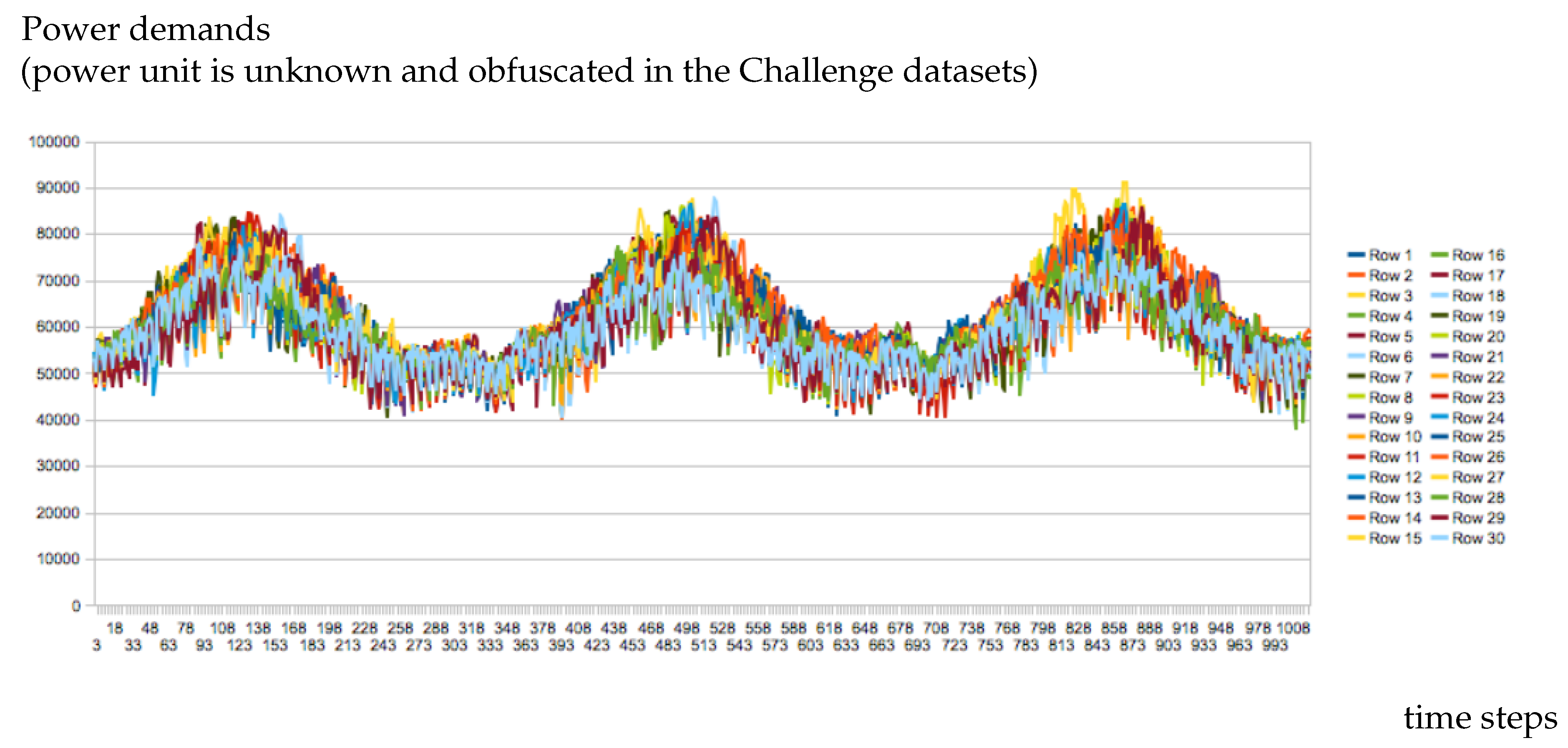
Power demands at time step t for the scenario s.
Da i , k Outage duration for maintenance and refueling at cycle k.
F t = F Conversion factor between power and fuel in time step t, constant in the data.
I c , w Maximal offline T2 power at week w for CT21 constraint c.
L i , k , c Latency in the resource requirement in CT19 constraint c for outage i , k .
N c , w Maximal number of outages under maintenance at week w for CT20 constraint c.
π s Probability of scenario s.
Pmin j , s , t Minimal power for T1 unit j at time period t and scenario s.
Pmax j , s , t Maximal power for T1 unit j at time period t and scenario s.
Pmax i , t Maximal generated power at time step t.
Q i , k Proportion of fuel that can be kept during reload in cycle k at plant i
R c 19 Maximal quantity of resource in CT19 constraint c.
Rmin i , k Minimal refueling at outage k.
Rmax i , k Maximal refueling at outage k.
S c Spacing/overlapping value defined by CT14-CT18 constraints.
Smax i , k Maximal fuel level at production cycle k.
t w Index of the first time step of week w.
Ta i , k Last possible beginning week for outage k of T2 plant i.
To i , k First, possible outage week for cycle k.
Tu i , k , c Length of the resource usage in CT19 constraint c for outage i , k .
w t Week of the production time step t.
Xi i Initial fuel stock of T2 plant i.
Table 3. Description of the constraints, with their references in the specification [14].
CT1: for all production time step t T and all scenario s S , the total production of T1 and T2 power plants must equalize the demands D s , t .
CT2: for all production time step t T and all scenario s S , the production domain of T1 plant j J describes exactly the continuous domain [ Pmin j , s , t , Pmax j , s , t ]
CT3: the productions of T2 power plants are null during the Da i , k weeks of outage ( i , k ) .
CT4-CT5: for each period t T and each scenario s S , the production domain of T1 plant j J describes exactly the continuous domain [ 0 , Pmax i , t ] when its fuel level is superior to Bo i , k .
CT7: the refueling level for outage k of T2 plant i describes the continuous domain [ Rmin i , k , Rmax i , k ] .
CT8: the initial fuel stock for T2 unit i is Xi i , known and common for all scenario s.
CT9: the fuel stock variation during a production campaign of a cycle ( i , k ) between t and t + 1 , is proportional to the power produced by i at time step t, with a proportional factor F t .
CT10: during an outage, the fuel stock variation is the sum of the refueling level and a certain amount of unspent fuel, calculated with a proportional loss with factor Q i , k < 1 to the residual fuel before refueling.
CT11: the fuel level is in [ 0 , Smax i , k ] for cycle k of T2 unit i. The fuel level must be lower than A i , k + 1 to process outage k + 1 .
CT13: outage ( i , k ) must begin between weeks To i , k and Ta i , k . The maintenance checks follow the order of set k K without skipping maintenance: if outage k + 1 is processed, it must follow the cycle k.
CT14: For all constraint c C 14 , a subset of outages, Z c have to be spaced by at least S c weeks: for S c > 0 , it is a minimal spacing from the beginning of a previous outage to the beginning of a next outage, for S c 0 , it is a maximal number of weeks where two outages can overlap.
CT15: CT15 are similar to CT14 with sets C 15 , Z c and parameters S c , applying only on a time interval W c .
CT16: for each constraint c C 16 , a subset of outages Z c have to be spaced by at least S c > 0 weeks from the beginning of the previous outage to the beginning of the next outage.
CT17: for each constraint c C 17 , a subset of outages Z c have to be spaced by at least S c > 0 weeks from the end of the previous outage to the end of the next outage.
CT18: for each constraint c C 18 , a subset of outages Z c have to be spaced by at least S c > 0 weeks from the end of the previous outage to the beginning of the next outage.
CT19: for each constraint c C 19 , a subset of outages ( i , k ) Z c shares a common resource (which can be a single specific tool or maintenance team) with forbid simultaneous usage of this resource. L i , k , c and Tu i , k , c indicate respectively the start and the length of the resource usage and R c 19 the maximal quantity of the resource.
CT20: for each constraint c C 20 , at most N c , w outages among a subset Z c overlap in weeks w W c .
CT21: for each constraint c C 21 , a time period W c is associated where the offline power of T2 plants I c I due to maintenance operations must be lower than I c , w .
Table 4. Definition of the variables for the MILP formulation relaxing only constraints CT6 and CT12.
d i , k , w { 0 , 1 } Binaries to indicate the beginning week for maintenance checks k of T2 unit i.
p i , k , s , t T 2 0 Power production of T2 unit i at cycle k at t for scenario s, 0 if t is not in cycle k.
p j , s , t T 1 0 Power production of T1 unit j at time step t for scenario s.
r i , k 0 Refueling quantity for outage k of T2 unit i.
x i , s e n d 0 Fuel stock of T2 unit i at the end of the optimizing horizon at scenario s.
x i , k , s i n i t 0 Fuel level at the beginning of production cycle k of T2 unit i.
x i , k , s f i n 0 Fuel level before the refueling k + 1 of T2 unit i, after production cycle k.
Table 5. Characteristics of the instances of the EURO/ROADEF Challenge 2010: values of I,J,K,S,T,W as defined in Table 1, nbVar0 and nbVar2 are respectively the total number of variables without and with pre-processing of Proposition 3, i.e., the total amplitude of the time windows, nbVar1 and nbVar3 are respectively the remaining variable after Cplex pre-processing with and without pre-processing of Proposition 3. Gaps show the improvements due to Proposition 3.
DataIJKSTWnbVar0nbVar1GapnbVar2nbVar3Gap
A110116101750250389246388.10%48342412.22%
A218216201750250788996187.82%89276114.69%
A318216201750250816287589.28%84169817.00%
A43031630175025017,465179889.71%1998149325.28%
A52831630175025015,357279781.79%275024949.31%
B65025650581727724,563346685.89%3467305411.91%
B74827650556526535,768643582.01%9052584635.42%
B856196121581727769,65322,48267.72%30,62620,76332.20%
B956196121581727769,30625,35163.42%35,30723,67532.95%
B1056196121556526529,948423685.86%5084379025.45%
X115025650581727720,081347882.68%349932168.09%
X124827650552326327,111434883.96%5321403524.17%
X1356196121581727730,154469784.42%440341046.79%
X1456196121581727730,691537882.48%6088487919.86%
X1556196121552326327,233399285.34%4372361817.25%
Table 6. Dual bounds for the dataset A, comparison of former dual bounds of the literature with the dual bounds L B ( k 0 ) with k 0 > 3 and L B without aggregation of production time steps and scenario decomposition. M indicates the maximal number of scenarios in sub-problems. MILP computation of dual bounds are stopped after 2400 × M seconds using Machine B. Bold values denote stopped computations with optimal dual bounds in the 0.001% tolerance for MILP computations. LP and LP + cuts are also the terminating values, no additional gap is implied by the time limit.
[16].1[16].2LB(4)LB(5)LBLBLBLBLBLB
MILPMILPLPLP + cutsMILPMILPMILPMILP
M = 1M = 1M = 1M = 1M = 1M = 2M = 3M = 5
A15.09%2.31%0.54%0.08%0.29%0.09%0.03%0.02%0.02%0.01%
A210.83%4.09%1.42%0.33%0.64%0.35%0.24%0.22%0.21%0.21%
A310.72%3.77%1.85%0.71%1.06%0.48%0.36%0.35%0.34%0.33%
A426.07%8.22%3.36%2.38%2.82%1.93%1.33%1.27%1.27%1.22%
A524.22%9.70%4.25%3.24%3.46%2.80%2.38%2.16%2.01%2.14%
Total14.20%5.24%2.11%1.19%1.49%1.00%0.77%0.71%0.68%0.69%
Table 7. Comparing with [16] the dual bounds using LP+cuts computations of L B ( k 0 ) with k 0 < 3 .
[16].1[16].2LB(1)LB(1)LB(2)LB(2)LB(3)LB(3)
GapGapt(s)Gapt(s)Gapt(s)Gap
B656.44%16.58%9914.95%21011.74%41911.67%
B752.86%15.58%8613.40%31011.18%95411.16%
B865.32%23.60%81120.34%448517.37%17.1k16.92%
B963.30%21.72%91118.78%441515.83%19k15.36%
B1060.92%18.03%28316.47%65013.43%130813.42%
X1157.81%15.40%11612.91%25711.18%47211.07%
X1252.65%14.22%11812.29%25710.30%57410.28%
X1366.20%18.53%31516.01%83214.28%166214.11%
X1464.67%17.21%34414.95%92613.23%176113.11%
X1561.76%16.83%37616.13%75613.52%137813.49%
Total60.15%17.80%345815.64%7.6k13.22%42.6k11.65%
Table 8. Comparing with [16] the dual bounds using MILP computations of L B ( k 0 ) with k 0 < 3 .
[16].1[16].2LB(0)LB(0)LB(1)LB(1)LB(2)LB(2)
GapGapt(s)Gapt(s)Gapt(s)Gap
B656.44%16.58%8218.12%12414.89%35611.67%
B752.86%15.58%6615.34%18113.39%99111.16%
B865.32%23.60%22123.12%121520.20%218k16.92%
B963.30%21.72%28221.73%177618.71%218k15.36%
B1060.92%18.03%22418.64%57316.46%103013.42%
X1157.81%15.40%9214.44%43612.84%126711.07%
X1252.65%14.22%11713.90%49612.27%113710.28%
X1366.20%18.53%26117.90%42415.86%170114.11%
X1464.67%17.21%27016.84%86114.87%388713.11%
X1561.76%16.83%42118.03%152816.10%693113.49%
Total60.15%17.80%203617.84%13k15.58%453k13.07%
Table 9. Comparison of our best dual bounds for datasets B and X allowing at most 1 h total computation to the ones from [16].
Primal[16]GapOur DualsGapt(s)ModelCutsM
B683,424.7 M69,592 M16.58%79,179.4 M5.09%3202LB(5)yes10
B781,099.7 M68,528 M15.58%76,139.8 M6.20%3529LB(5)yes5
B881,899.7 M62,59423.60%67,352.4 M17.79%1521LB(2)no1
B981,689.5 M63,99121.72%68,566.3 M16.13%1602LB(2)no1
B1077,767.0 M63,74718.03%72,213.9 M7.14%2040LB(5)yes2
∑ B405,880.6 M328,452 M19.11%363,452 M10.49%
X1179,007.6 M66,93115.40%74,431.2 M5.92%1209LB(5)yes2
X1277,564.0 M66,55814.22%72,819.4 M6.15%3449LB(5)yes10
X1376,288.5 M62,15518.53%70,236.7 M7.93%1735LB(5)no1
X1476,149.8 M63,04517.21%70,279.3 M7.71%1741LB(5)no1
X1574,388.4 M61,86616.83%68,624.8 M7.75%3045LB(5)yes3
∑ X383,531.7 M320,555 M16.42%35,639 M7.08%
Total789,572.7 M649,007 M17.80%719,843.6 M8.83%
Table 10. Dual bounds for datasets B and X, computing L B ( k 0 ) with k 0 > 3 and LB bounds with M = 1 scenario decomposition, using truncated LP, LP+cuts, and MILP computations.
[16]LB(4)LB(4)LB(4)LB(5)LB(5)LB(5)LBLB
LPLP + cutsMILPLPLP + cutsMILPLP + cutsMILP
B616.58%7.24%7.06%6.84%5.67%5.48%5.31%5.48%5.07%
B715.58%7.68%7.54%7.23%6.82%6.68%6.34%7.99%7.55%
B823.60%13.86%13.68%13.52%12.75%12.41%12.22%16.16%16.16%
B921.72%12.70%12.55%12.40%11.96%11.72%11.51%15.81%15.81%
B1018.03%8.53%8.41%8.33%7.52%7.39%7.32%7.53%7.01%
X1115.40%7.95%7.81%7.64%6.33%6.17%6.04%5.66%5.36%
X1214.22%7.58%7.50%7.42%6.81%6.73%6.68%6.88%6.49%
X1318.53%10.74%10.37%10.12%8.65%8.31%8.14%7.82%7.46%
X1417.21%10.00%9.81%9.62%8.27%8.06%7.91%8.10%7.76%
X1516.83%10.21%10.11%10.02%9.06%9.16%8.99%9.11%8.82%
Total17.80%9.65%9.49%9.32%8.40%8.21%8.05%9.09%8.79%
Table 11. Dual bounds for datasets B and X, computing of dual bounds LB(5) and LB with LP+cuts computations, aggregation of production time steps and scenario decomposition varying M the maximal number of scenarios in each sub-problem.
[16]LB(5)LBLB(5)LBLB(5)LB
M= 112233
B616.58%5.48%5.48%5.26%5.30%5.19%5.26%
B715.58%6.68%7.99%6.37%7.81%6.28%7.79%
B823.60%12.41%16.16%12.13%16.23%12.05%16.14%
B921.72%11.72%15.81%11.47%15.76%11.39%15.70%
B1018.03%7.39%7.53%7.14%7.33%7.05%7.25%
X1115.40%6.17%5.66%5.92%5.42%5.83%5.34%
X1214.22%6.73%6.88%6.43%6.58%6.31%6.50%
X1318.53%8.31%7.82%8.03%7.53%7.93%7.44%
X1417.21%8.06%8.10%7.76%7.81%7.66%7.73%
X1516.83%9.06%9.11%8.74%8.78%8.62%8.69%
Total17.80%8.21%9.09%7.94%8.90%7.84%8.83%
[16]LB(5)LBLB(5)LBLB(5)LB
M= 11551010
B616.58%5.48%5.48%5.13%5.23%5.09%5.21%
B715.58%6.68%7.99%6.20%7.76%6.14%7.76%
B823.60%12.41%16.16%11.97%16.16%11.95%16.15%
B921.72%11.72%15.81%11.32%15.75%11.24%15.73%
B1018.03%7.39%7.53%6.96%7.21%6.90%7.18%
X1115.40%6.17%5.66%5.76%5.29%5.71%5.27%
X1214.22%6.73%6.88%6.20%6.41%6.15%6.35%
X1318.53%8.31%7.82%7.85%7.34%7.81%7.31%
X1417.21%8.06%8.10%7.57%7.69%7.50%7.65%
X1516.83%9.06%9.11%8.52%8.60%8.46%8.56%
Total17.80%8.21%9.09%7.76%8.79%7.70%8.76%
Table 12. New best dual bounds for EURO/ROADEF Challenge 2010, comparison to the former ones of [16,17], and presenting the configuration leading to our best lower bounds. Gaps are calculated for the best primal solution known from [15,28,32]. Machine A is used for instances of datasets B and X, whereas Machine B was used for the instances of datasets A.
Primal [16].1[16].2[17]New Lower BoundGapBoundMTime/S
A1169,474.5 M[32]5.09%2.31%0.04%169,460.6069 M0.01%LB10OPT
A2145,956.7 M[32]10.83%4.09%0.25%145,669.1154 M0.20%LB10OPT
A3154,277.2 M[32]10.72%3.77%0.37%153,770.2050 M0.33%LB10OPT
A4111,494.0 M[15]26.07%8.22%1.52%110,130.2886 M1.22%LB52400
A5124,543.9 M[15]24.22%9.70%2.55%122,035.5788 M2.01%LB32400
∑ A705,746.3 M 14.20%5.24%0.83%701,065.7947 M0.66%
B683,424.7 M[28]56.44%16.58%5.30%79,394.9322 M4.83%LB53600
B781,099.7 M[15]52.82%15.50%6.22%76,499.2099 M5.67%LB(5)103600
B881,899.7 M[15]65.31%23.57%12.37%72,322.5889 M11.69%LB(5)103600
B981,689.5 M[15]63.28%21.67%11.59%72,811.7201 M10.87%LB(5)103600
B1077,767.0 M[15]60.92%18.03%7.32%72,462.8317 M6.82%LB(5)101800
∑ B405,880.6 M 59.74%19.08%8.56%373,491.2828 M7.98%
X1179,007.6 M[15]57.75%15.29%5.45%75,183.0108 M4.84%LB53600
X1277,564.0 M[15]52.63%14.19%6.65%72,986.7523 M5.90%LB53600
X1376,288.5 M[15]66.20%18.53%7.59%70,988.40356 M6.95%LB51800
X1476,149.8 M[15]64.67%17.21%7.82%70,549.09524 M7.35%LB51800
X1574,388.4 M[15]61.76%16.83%8.11%68,821.7327 M7.48%LB51800
∑ X383,398.3 M 60.55%16.39%7.11%358,421.1372 M6.49%
∑ BX789,278.9 M 60.13%17.77%7.85%731,912.4200 M7.25%
Total1,495,025.2 M 38.45%11.85%4.54%1,432,978.2147 M4.14%

