Generative Model for Skeletal Human Movements Based on Conditional DC-GAN Applied to Pseudo-Images

Abstract

Generative models for images, audio, text, and other low-dimension data have achieved great success in recent years. Generating artificial human movements can also be useful for many applications, including improvement of data augmentation methods for human gesture recognition. The objective of this research is to develop a generative model for skeletal human movement, allowing to control the action type of generated motion while keeping the authenticity of the result and the natural style variability of gesture execution. We propose to use a conditional Deep Convolutional Generative Adversarial Network (DC-GAN) applied to pseudo-images representing skeletal pose sequences using tree structure skeleton image format. We evaluate our approach on the 3D skeletal data provided in the large NTU_RGB+D public dataset. Our generative model can output qualitatively correct skeletal human movements for any of the 60 action classes. We also quantitatively evaluate the performance of our model by computing Fréchet inception distances, which shows strong correlation to human judgement. To the best of our knowledge, our work is the first successful class-conditioned generative model for human skeletal motions based on pseudo-image representation of skeletal pose sequences.

1. Introduction

Human movement generation, although less developed than for instance text generation, is an important applicative field for sequential data generation. It is difficult to get enough effective human movement dataset due to its complexity—human movement is the result of both physical limitation (torque exerted by muscles, gravity, and moment preservation) and the intentions of subjects (how to perform an intentional motion) [1]. Generating artificial human movement data enables data augmentation, which should improve the performance of models in all fields of study on human movement: classification, prediction, generation, etc. Also, it will have important applications in related domains. Imagine, for example, in computer games, each character running and jumping in exactly the same way but in their own style, making those actions in the game closer to reality.

The objective of this research is to develop a generative model for skeletal human movements, allowing to control the action type of generated motion while keeping the authenticity of the result and the natural style variability of gesture execution. Skeleton-based movement generation has recently become an active topic in computer vision, owing to the potential advantages of skeletal representation and to recent algorithms for automatically extracting skeletal pose sequences from videos. Previously, most of the methods and researches on human gestures, including human movement generation, used RGB image sequences, depth image sequences, videos, or some fusion of these modalities as input data. Nowadays, it is easy to get relatively accurate 2D or 3D human skeletal pose data thanks to state-of-the-art human pose estimation algorithms and high-performance sensors. Compared to dense image approaches, skeletal data has the following advantages: (a) lower computational requirement and (b) robustness under situations such as complicated background and changing body scales, viewpoints, motion speed, etc. Besides these advantages, skeletal data has the three following main characteristics [2]:

• spatial information: strong correlations between adjacent joints, which makes it possible to learn about body structural information within a single frame (intra-frame);
• temporal information: makes it possible to learn about temporal correlation between frames (inter-frame); and
• cooccurrence relationship between spatial and temporal domains when taking joints and bones into account.

Skeletal-based human movement generation can be formalized as a continuous multivariate time-series problem and is therefore often tackled using Recurrent Neural Network (RNN). In our work, we however decided to use representation of each skeletal pose sequence as a spatiotemporal pseudo-image with space and time as two dimensions of the image instead. The advantage is that we can directly apply state-of-the-art generative models for images, which are more mature and simpler in terms of the network architecture than the ones tailored for continuous time-series generation. Thus, it is important to find a good pseudo-image representation for 3D skeletal data. The related works will be further developed in the next part. The key issues to be solved include how to generate realistic human movements, how to control the output (action, style, etc.), and how to evaluate the model effectively.

Our work proves that, as long as we apply a well-adapted pseudo-image representation for 3D skeletal data, such as Tree Structure Skeleton Image (TSSI), we can generate human movement by a simple standard image generative model such as Deep Convolutional Generative Adversarial Network (DC-GAN [3]). Furthermore, by introducing a conditional label, we control the output action type. We also evaluate our generative models by calculating Fréchet inception distance.

The paper is organized as follows: Section 2 presents published works related to human movement generative models and to pseudo-image representations for skeletal pose sequences; Section 3 explains the details of our approach; Section 4 analyzes the results we have obtained; and Section 5 presents our conclusions and perspectives.

2. Related Works

In this section, we present some of the already published works most related to our work concerning generative models for skeletal human movements and pseudo-image representation for skeletal pose sequences.

2.1. Generative Models for Skeletal Human Movements

A family of methods based on deep Recurrent Neural Networks (RNNs) have shown good performance on generative tasks for human skeletal movements. For example, Fragkiadaki et al. [4] proposed in 2015 the Encoder-Recurrent-Decoder (ERD) model that uses curriculum learning and incorporates representation learning in the architecture. In 2016, Jain et al. introduced the concept of structural-RNN [5], which manually encodes the semantic similarity between different body parts based on spatiotemporal graphs. The reason why RNN is a popular generative model for sequential data is that RNNs typically possess both a richly distributed internal state representation and flexible nonlinear transition functions. This expressive power and the ability to train via error back-propagation are the key reasons why RNNs have gained popularity as generative models for highly structured sequential data. Inspired by previous works on RNN, Martinez et al. [1] proposed in 2017 a human motion prediction model using sequence-to-sequence (seq2seq) architecture with residual connections, which turned out to be a simple but state-of-the-art method on prediction of short-term dynamics of human movement. Chung et al. [6] explored the inclusion of the latent random variables into the hidden state of an RNN by combining the elements of the variational autoencoder. They argued that, through the use of high-level latent random variables, their variational RNN (VRNN) can model the kind of variability observed in highly structured sequential data such as natural speech.

Besides the models based on RNNs and Variational Auto-Encoders (VAEs), Generative Adversarial Networks (GANs) [7], which achieve great success in generative problems, are recently one of the most active machine-learning research topics. GANs have proved their strength in the generation of images and some types of temporal sequences. For example, Deep Convolutional GAN (DC-GAN) [3] proposed a strided conv-transpose layer and introduced a conditional label, which allows for the generation of impressive images. WaveNet [8], applying dilated causal convolutions that effectively operate on a coarser scale, can generate raw audio waveforms and can transform text to speech which human listeners can hardly distinguish from the true voice. Recently, several researches on human movement prediction and generation models are based on GAN. In 2018, the Human Prediction GAN (HP-GAN) [9] of Barsoum et al. used also a sequence-to-sequence model as its generator and additionally designed a critic network to calculate a custom loss function inspired by WGAN-GP [10]. Kiasari et al. [11] approached from another way the combination of an Auto-Encoder (AE) and a conditional GAN to generate a sequence of human movements.

2.2. Pseudo-Image Representation for Skeletal Pose Sequences

In many skeleton-based human movement recognition studies, researchers use Convolutional Neural Networks (CNN) because of their efficiency and excellent ability to extract high level information. However, the most common and developed CNNs use 2D convolutions and therefore generally focus on image-based tasks. Meanwhile, human movement problems, including recognition and, the main task of this paper, generation, are definitely a heavily temporal problem. Thus, it is challenging to balance and capture both spatial and temporal information in a CNN-based architecture [2].

In general, to meet the needs of the CNN input, a 3D skeletal sequence data should be transformed into a pseudo-image. Nevertheless, a decent representation that contains both spatial and temporal information is not simple. Many researchers encode the skeletal joints to multiple 2D pseudo-images and then feed them into the model. Wang et al. [12] introduced Joint Trajectory Maps (JTM), which represent spatial configuration and the dynamics of joint trajectories into three texture images through color encoding. Li et al. [13] proposed a translation-scale invariant image mapping. They pointed out that the JTM encoding method is dataset dependent and not robust to the translation and scale variation of human activity. To tackle this problem, they divided all human skeletal joints into five main parts according to human physical structure and then mapped them to images. However, they merely focused on the coordinates of isolated joints and therefore ignored the spatial relationships between joints and only implicitly learned the movement representations. Take the action “walking” for example, not only the legs and feet but also the arms and other body parts should be considered. In a word, the human body needs to be treated as a whole. To solve this problem, Li et al. [14] proposed in 2019 an effective method to learn comprehensive representations from skeletal sequences by using geometric algebra. Firstly, a frontal orientation-based spatiotemporal model was constructed to represent the spatial configuration and temporal dynamics of skeletal sequences, which is robust against view variations. Then, shape-motion representations which mutually compensate one another were learned to describe the skeletal actions comprehensively. Liu et al. [15] used enhanced skeletal visualization to represent the skeletal data. SkeleMotion [16] directly encodes data by using orientation and magnitude to provide information regarding the velocity of the movement in different temporal scales. The Tree Structure Reference Joint Image (TSRJI) of Caetano et al. [17] combines the use of reference joints and a tree structure skeleton: while the former incorporates different spatial relationships between the joints, the latter preserves important spatial relations by traversing a skeletal tree with a depth-first order algorithm.

Even if these skeletal sequence representations have made great efforts to encode as much information as possible in one or a series of “images”, it is still hard to learn global cooccurrences. When these pseudo-images are fed to CNN-based models, only the neighboring joints within the convolutional kernel are considered with learning local cooccurrence features. Thus, in 2018, Li et al. [18] proposed an end-to-end cooccurrence feature-learning framework, where features are aggregated gradually from point-level features to global cooccurrence features.

3. Materials and Methods

To generate human skeletal motions, we used a conditional Deep Convolutional Generative Adversarial Network (DC-GAN) applied to pseudo-images representing skeletal pose sequences using Tree Structure Skeleton Image (TSSI) format. We evaluated our approach on the 3D skeletal sequence data provided in the large NTU_RGB+D [19] public dataset, and use Fréchet inception distances as quantitative evaluation. The details of the database, pseudo-image representation, data preparation, our generative model, and the process of training and evaluation will be provided in this section.

3.1. NTU_RGB+D Dataset

NTU_RGB+D [19] is a large-scale public dataset for 3D human activity analysis. It contains 60 different action classes including daily, mutual, and health-related actions. With 56,880 samples, 40 human subjects, and 80 camera views, this dataset is much larger than other available datasets for RGB+D (RGB videos and depth sequence) action analysis. In our research, we only use the skeletal data (3D locations of 25 major body joints) provided in the dataset.

3.2. Tree Structure Skeleton Image (TSSI)

In our approach, we transform the skeletal pose sequences into Tree Structure Skeleton Image (TSSI) pseudo-images [20]. The principle of TSSI is to create one image for each sequence of skeletons. In these spatiotemporal pseudo-images, the horizontal axis corresponds to joint positions and the vertical axis corresponds to time. The joint positions are encoded as one channel for x, one for y, and one for z, therefore obtaining a color image with red corresponding to x, green corresponding to y, and blue corresponding to z. One of the important particularities of TSSI is reordering the skeletons using depth-first tree traversal order so that neighboring columns in spatiotemporal images are spatially related in the original skeletal graph. The spatial relations between connected skeletal joints can thus be well preserved. TSSI can be trained with semantical meaning in a normal generative model for images, where the spatial and temporal features are meant to be learnt at the same time. Also, compared with other pseudo-image methods, TSSI is relatively simple. Figure 1 illustrates the skeleton structure and order in NTU_RGB+D with traversal order and joint arrangements of TSSI.

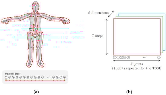
Figure 1. Illustration (adapted from [20]) of Tree Structure Skeleton Image (TSSI): (a) skeleton structure and order in NTU_RGB+D, with traversal order that respects spatial relations, and (b) joint arrangements of TSSI. The shape is (T, J, d) where T is the sequence duration, J’ the number of joints in traversal order (J joint repeated for the TSSI), and d the dimension (d = 3 for (x, y, z) 3D positions).

3.3. Data Preparation

First, we cleaned up the samples with missing data. Next, since the time length of sequences in NTU_RGB+D varies around 100 frames, we linearly resampled all examples to the length of 100 time-steps. They were then transformed into TSSI pseudo-images of size 100 × 49 × 3 (time, joints in TSSI order, 3), where 3 stands for the three-dimensional coordinates of each joint. The input size of DC-GAN was 64 × 64 × 3. Thus, the spatiotemporal images were further resized to 64 × 64 × 3 using bilinear interpolation. Finally, these images were saved by class. The entire dataset was used for training.

3.4. Conditional Deep Convolution Generative Adversarial Network (Conditional DC-GAN)

In this paper, we used a conditional Deep Convolution Generative Adversarial Network (conditional DC-GAN) based on DC-GAN [3] and cGAN [21]. In the original DC-GAN architecture, the discriminator was made up of strided convolution layers, batch norm layers, and LeakyReLU activations. Its input was a 64 × 64 × 3 (Height × Width × Channel) image, and the output was a scalar probability that the input is from real-data distribution. The generator was comprised of convolutional-transpose layers, batch norm layers, and ReLU activations. Its input was a latent vector z, that was drawn from a standard normal distribution, and the output was a 64 × 64 × 3 RGB image. The strided conv-transpose layers allowed the latent vector to be transformed into a volume with the same shape as an image.

Figure 2 shows the architecture of our conditional DC-GAN. In the generator, we used an upsample layer and a convolutional layer instead of the original convolutional-transpose layer in order to avoid checkerboard artifacts [22]. If a standard deconvolution (based on convolutional-transpose layer) is used to upscale from a lower resolution image to a higher one, it uses every point in the small image to “paint” a square in the larger one. Here comes the problem of “uneven overlap”, that is to say, when these “squares” in the larger image overlaps. In particular, deconvolution has uneven overlap when the kernel size is not divisible by the stride. These overlapped pixels create an unwanted checkerboard pattern on generated images.

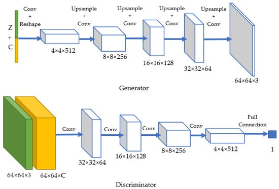
Figure 2. Architecture of our conditional Deep Convolutional Generative Adversarial Network (DC-GAN).

Thus, we instead used an upsample layer followed by convolutional layers to achieve the “deconvolution” operation. We resized the image, using the upsample layer with bilinear interpolation (or nearest-neighbor interpolation) and then using a convolutional layer. For the best result, before the convolutional layer, we added a RelectionPad2d layer of size 1 to avoid boundary artifacts. Details are provided in Appendix A.

In order to control the output action, the model receives the class label at input for both the generator and discriminator. The generator receives as input a random noise (1 × 1 × Z) and a one-hot conditional label (1 × 1 × C), where Z is the dimension of z and C is the number of classes. By default, we chose Z = 100 and C = 60. They were concatenated and passed to a convolutional layer, with a 1 × 1 kernel. The output channel was 8192 (=4 × 4 × 512). Then, the output data were resized to the shape of 4 × 4 × 512. Finally, we passed the data to several upscaling blocks (Upsample + Conv2D + BatchNorm, except for the output layer), which is exactly the same as the ones in the original DC-GAN. The reason for not directly resizing the input data (the concatenation of random noise and one-hot label) was that, when the data size is 1 × 1, it can only be upsampled to an equal-valued data. Also, we wished to keep the input noise size at 1 × 1 × Z. Therefore, we decided to add an extra convolutional layer and the resizing step to make it work. In the discriminator, the label was encoded as an image with C channels (C for class number). The label was one-hot encoded along the dimension of channel. To be more specific, the label of the nth action was an H × W × C sized data, with all 1s on the nth channel and 0 for the rest. At the input layer, the image and the label were concatenated: every pixel of the image was concatenated with a one-hot label in the direction of channel. Thus, the input channel size was 3 + C. The architecture of the discriminator consisted in several convolutional layers and batch normalization layers (except for the output layer) as in the the original architecture of DC-GAN.

3.5. Loss Function and Training Process

We used the standard loss function for GANs, which is defined in [7] as follows:

$$\underset{G}{\min } \underset{D}{\max }V\left(D,G\right)={\mathbb{E}}_{x~p_{data}}\left(x\right)\left[\log D\left(x\right)\right]+{\mathbb{E}}_{x~p_z}\left(z\right)\left[\log \left(1-D\left(G\left(x\right)\right)\right)\right]$$

(1)

Since a GAN has a generator and a discriminator, we had two losses: Loss_D and Loss_G. We used the Binary Cross Entropy (BCE) as loss functions. Loss_D was calculated as the sum of errD_real = $-\log \left(D\left(x\right)\right)$ and errD_fake = $-\log \left(1-D\left(G\left(z\right)\right)\right)$, representing the BCE of the prediction to the reality when D receives real inputs and fake inputs. Loss_G = $-\log \left(D\left(G\left(z\right)\right)\right)$ calculates the BCE of the “false positive” prediction when D receives fake inputs.

The discriminator and the generator were trained and updated one after another, with the adam optimizer at learning rate = 0.0002 by default.

3.6. Transformation of Generated Pseudo-Images into Skeletal Sequences

The input and output data of our model were both pseudo-images. In Section 3.3, we explain how we transform the original skeletal variable-length sequences into TSSI pseudo-images with all the same size, which are fed into the discriminator. The generator produces fake pseudo-images with the same size. Therefore, in order to obtain a sequence of skeletons from the generated pseudo-image, we need to perform a symmetric operation of that described in Section 3.3. First, the generated 64 × 64 × 3 pseudo-image was resized into 100 × 49 × 3 (time-step, joints in TSSI order, xyz) using bilinear interpolation (we chose 100 time-steps as the unique length for generated sequences). Then, for the joints which were repeated in TSSI order, we took the average value. For example, the third joint (neck) was repeated twice in TSSI order (the third and the fourth). We calculated the average of these two values and took it as the value of the third joint of skeleton. In this way, for each generated pseudo-image, we obtained a corresponding generated skeletal sequence with a shape of 100 × 25 × 3 (time-steps, joints, xyz), which can be visualized as a sequence of skeletal poses.

3.7. Model Evaluation—Fréchet Inception Distance (FID)

To evaluate the model, we used Fréchet Inception Distance (FID) [23]. FID is a measure of similarity between two datasets of images. It was shown to correlate well with human judgement of visual quality and is most often used to evaluate the quality of samples of GAN. FID was first proposed and used in [24] to improve the evaluation, being more consistent than the inception score [25]. The FID metric calculates the distance between two distributions of images on the level of features. As in [25], we computed FID measures using the features extracted from a pretrained inception V3 model [26]. FID is calculated by the following function [23]:

$$\mathrm{FID}={\Vert {\mu }_r-{\mu }_g\Vert }^2+Tr\left({\mathsf{\Sigma }}_r+{\mathsf{\Sigma }}_g-2{\left({\mathsf{\Sigma }}_r{\mathsf{\Sigma }}_g\right)}^{1/2}\right)$$

(2)

${\mu }_r, {\mu }_g$ are the mean values of features of real and fake images

${\mathsf{\Sigma }}_r, {\mathsf{\Sigma }}_g$ are the covariance matrix of features of real and fake images

The smaller the FID, the greater the similarity between the two distributions. In our study, the real images were the TSSI pseudo-images obtained (as described in Section 3.3) from skeletal sequences of the NTU_RGB+D dataset and the fake images were the pseudo-images generated by our generative model. We calculated FID between these two distributions of data as a metric. The aim was to minimize FID.

Since we would like to evaluate the performance both by class of action and by all actions in the future, we prepared the statistics for each class of action and the whole dataset. When calculating FID, we only need to generate a certain number of fake samples to get its statistics ${\mu }_g$ and ${\mathsf{\Sigma }}_g$. Notice that there is a tradeoff between the fake sample numbers and computational cost of evaluation. The more generated samples, the better the distribution of fake samples are presented. Meanwhile, it spends more time and calculation power. Thus, it is crucial to decide the number of samples. We chose to generate 250 samples for each class of action.

4. Results

4.1. Qualitative Result for Generated Skeletal Actions

We first analyze qualitatively the results of our generative model. Figure 3 shows four examples of actions generated by our model (with default hyperparameter setting) trained after 200 epochs: (a) sitting down; (b) standing up; (c) hand waving; and (d) kicking something. For each action class, the figure also shows for comparison a typical real pose sequence from the training set. As can be seen, the generated skeletal sequences match qualitatively and visually with the typical training example of a real pose sequence for the action class corresponding to the value of the class-condition input fed into our generator. The respective characteristics of each action class, such as the movement of body parts, are correctly learnt by the model, and the generated movements are continuous and smooth.

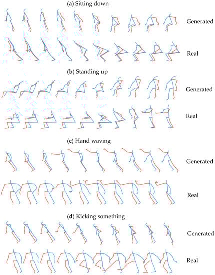
Figure 3. Examples of generated actions compared with a typical real training sequence for 4 action classes: (a) sitting down, (b) standing up, (c) hand waving, and (d) kicking something.

4.2. Quantitative Model Evaluation Using Fréchet Inception Distance (FID)

At each evaluation, we record the FID score for each class of action, their average value, and the FID score of the total dataset. Figure 4 shows the action “standing up” generated by our model at the 150th epoch and the 200th epoch. The FID score is much smaller at the 200th epoch, and the corresponding generated sequence is obviously qualitatively (i.e., visually) better. This confirms that the FID on pseudo-images is clearly a good measure of the quality of the corresponding generated pose sequences.

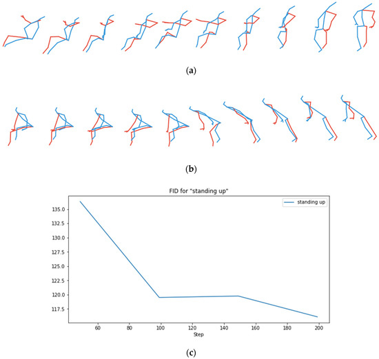
Figure 4. Checking the consistency of the Fréchet Inception Distance (FID) score with the qualitative appearance of generated action: the action “standing up” generated by the model after (a) 150 epoch training and (b) 200 epoch training, and (c) the corresponding curve of FID as a function of training epochs.

We now show in Figure 5 some FID scores during the training of our model, evaluating every 50 epochs. The first two rows of curves stand for 8 different actions and the last two curves are the class average FID and the FID for the entire dataset. For most actions, the FID score globally decreases as training goes on. It theoretically means that, as training goes on, the generated pseudo-images get closer to the real TSSI training pseudo-images in terms of realness and diversity. We however note that, for some action classes, the FID increases again after the 150th epoch. The same trend is visible on the average FID score. This means that, in general, for one class of action, the results are better for the model trained after 150 epochs than after 200 epochs. When regarding all actions as a whole, we can derive the same conclusion with the total FID score.

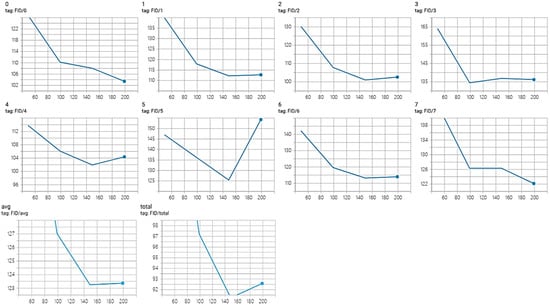
Figure 5. FID curves evaluated on (0–7) 8 different actions, (avg) their average score, and (total) the entire dataset.

4.3. Importance of the Modification of Generator Using Upsample + Convolutional Layers

As explained in Section 3.4, we modified the deconvolution operation from the original DC-GAN in order to avoid checkerboard artifacts that arise when using simply convolutional-transpose layers. To tackle this problem, we applied the upsample + convolutional layer method to realize the deconvolution operation. In Figure 6, we compare the learning curves (Loss_D and Loss_G) of our model (orange) with the original conditional DC-GAN model (blue) trained with the same input. Our model converges much faster than the original one, meaning that the new model is much easier to train.

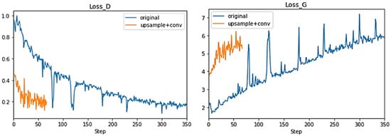
Figure 6. Learning curves of our model (using upsample and convolutional layers) (orange) and the original method (using convolutional-transpose layers) (blue): Loss_D is discriminator loss calculated as the average of losses for the all real and all fake samples, and Loss_G is the average generator loss.

Furthermore, we visually inspect some generated pseudo-images in order to check the improvement. On Figure 7, we compare a real TSSI input pseudo-image on Figure 7a; a fake pseudo-image generated by the original conditional DC-GAN model with convolutional-transpose layers, having checkerboard patterns on the entire image on Figure 7b; and a fake pseudo-image without checkerboard artifacts generated with our modified DC-GAN on Figure 7c. This confirms that, thanks to our modification of upsampling in the generator, the checkerboard pattern artifact no longer appears.

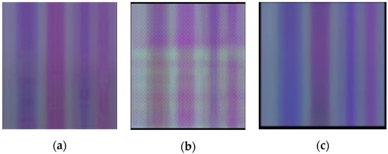
Figure 7. Example of spatiotemporal images: (a) TSSI of a real sequence; (b) an image generated by the original conditional DC-GAN model with convolutional-transpose layers, with checkerboard artifacts; and (c) an image generated by our model, without checkerboard artifacts.

In order to check how essential it is for our approach to avoid checkerboard artifacts, we finally compare the corresponding generated actions. Figure 8 shows the action “drinking” generated by (a) new model-trained 69 epochs and (b) original models after 349 epochs when the learning curves of two models reach the same values. Comparing those two generated sequences of the action “drinking”, the former is obviously more continuous and realistic. The human skeleton is closer to reality as well. The body shape deformations and action unsmoothness visible in Figure 8b are the consequences of the checkerboard artifacts in the generated pseudo-image, which translate into very bad pose sequences after reconverting from TSSI pseudo-image.

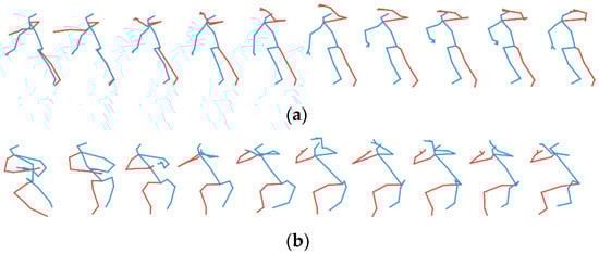
Figure 8. Sequence of action “drinking” generated by (a) our model (using upsample + convolutional layers) trained after 69 epochs and (b) the original model (using convolutional-transpose layer) trained after 349 epochs.

In conclusion, our analysis confirms that, for our work, using the upsample + convolutional layer structure to realize deconvolution in the generator is efficient and essential for obtaining realistic generated sequences of skeletons.

4.4. Importance of Reordering Joints in TSSI Spatiotemporal Images

In order to assess the importance of joint reordering in TSSI skeletal representation, we also train our generative model using pseudo-images without tree traversal order representation. The spatial dimension is then simply the joint order from 1 to 25. Figure 9 compares the actions generated by the two trained models, without or with TSSI representation. Figure 9a is the training result by non-TSSI images, and Figure 9b is the result trained by TSSI. It is obvious that, after the same training epochs, the model obtained using non-TSSI pseudo-images cannot output a realistic human skeleton.

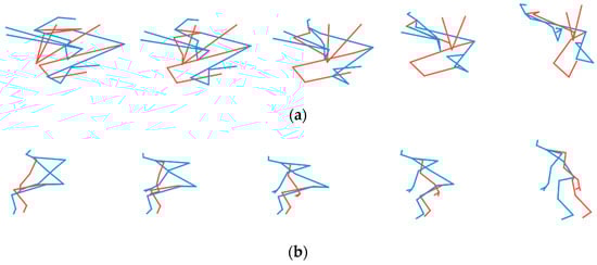
Figure 9. Sequences of action “standing” generated by the models trained (a) with non-TSSI pseudo-images (no reordering of joints) and (b) with TSSI-reordered pseudo-images.

4.5. Hyperparameter Tuning

After justifying the choice of our model architecture and data format, we explore the effect of hyperparameter values: learning rate, batch size, and number of dimensions of latent space z. By default, we set learning rate at 0.0002, batch size at 64, and dimension of z at 100. Figure 10 shows the learning curves for the model trained with different learning rates: 0.001, 0.0005, 0.0002, and 0.0001. Opposite to common sense, when the learning rate is smaller, Loss_D and Loss_G converge faster. For models lr = 0.001 and lr = 0.0005, the average FID for a single class reaches the minimum at the 150th epoch and then goes up at the 200th epoch. For model lr = 0.0002, FID scores increase slightly at the 200th epoch. For model lr = 0.0001, FID scores keep decreasing but converge slowly. For all four models, FID scores are close to each other at the 200th epoch.

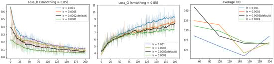
Figure 10. Learning curves for our model trained with different learning rates: 0.001, 0.0005, 0.0002, and 0.0001.

We also train the model with different batch sizes (of training data): 16, 32, 64, and 128 (see Figure 11). When the batch size is small, the learning curves Loss_D and Loss_G are smoother and the discriminator learns more easily However, FID score converges clearly best with batch size = 64.

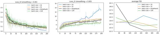
Figure 11. Learning curves for our model trained with different batch sizes (of input data): 16, 32, 64, and 128.

Finally, we investigate the influence of the dimension dim_z of the latent space z. In Figure 12, Loss_D and Loss_G are not affected by the choice of dim_z while FID scores vary significantly. With the increase of dim_z, FID scores tend to converge faster. For the model with dim_z = 5, the FID score shows the decreasing trend along 200 epochs. For the model with dim_z = 10 and 30, the FID scores both reach the minimal value near the 150th epoch and then go up. The model with dim_z = 100 gets the lowest point of FID at the 130th and 180th epochs, much smaller than the results of the others. However, further training epochs are needed to figure out whether FID for dim_z = 5 and 100 would continue decreasing.

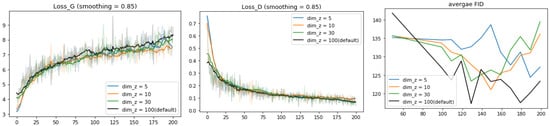
Figure 12. Learning curves for the model trained on different numbers of dimensions of the latent space z (input of G): 5, 30, and 100. For the average FID, we plot the value at 50, 100, 110, 120, 200 epochs.

To sum up, when training the model at 200 epochs, the original choice of the learning rate and batch size is already a relatively good setup. Regarding the optimal dimension of latent space, further study is needed to determine it robustly.

4.6. Analysis of Latent Space

We now analyze the influence of the latent variable z on the style of generated pose sequences. To this end, we move separately along each dimension of the latent space and try to understand the specific influence of each z coordinate on the appearance of generated sequences. In Figure 13, we visualize the variation with z of the generated action “standing up”. The model is trained after 200 epochs with dim_z = 5. For each figure, we adopt linear interpolation on one dimension of z, with 5 points in the range of [−1, 1]. Each row is the sequence generated by an interpolation “point” of latent space z. By comparing the first frame of each sequence (the first column), it seems that latent space z influences in particular the initial orientation of the skeleton. For instance, in Figure 13, the body rotates from the front to its right side (or the left side from the reader’s point of view). The evolution from top to bottom is continuous and smooth. At the same time, for each row of the sequence, the action “standing up” is performed well. This example shows that, by tuning on latent space z, our generative model is able to continuously control properties, such as the orientation, of the action and eventually to define the style of action while generating the correct class of action indicated by the conditional label.

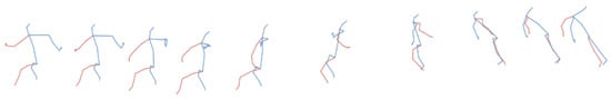
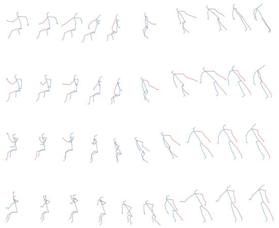
Figure 13. Variation of the generated action “standing up” with varying values of latent vector z.

5. Conclusions

In this work, we propose a new class-conditioned generative model for human skeletal motions. Our generative model is based on TSSI (Tree Structure Skeleton Image) spatiotemporal pseudo-image representation of skeletal pose sequences, on which is applied a conditional DC-GAN to generate artificial pseudo-images that can be decoded into realistic artificial human skeletal movements. In our setup, each column of a pseudo-image corresponds to approximately one single skeletal joint, so it is quite essential to avoid artifacts in the generated pseudo-image; therefore, we modified the original deconvolution operation in standard DC-GAN in order to efficiently eliminate checkerboard artifacts.

We evaluated our approach on the large NTU_RGB+D human actions public dataset, comprising 60 classes of actions. We showed that our generative model is able to generate artificial human movements qualitatively and visually corresponding to the correct action class used as the condition for the DC-GAN. We also used Fréchet inception distance as an evaluating metric, which quantitatively confirms the qualitative results.

The code of our work will soon be made available on Github. As further works, we will continue to improve the quality of generated human movements, for instance, adding a conditional label in every hidden layer in the network [27] and evaluating the performances, and trying or developing other representations of skeletal pose sequences. Moreover, evaluation of the model on other human skeletal datasets is important to verify the universality of the model.

References

- Martinez, J.; Black, M.J.; Romero, J.; IEEE. On human motion prediction using recurrent neural networks. In Proceedings of the 30th IEEE Conference on Computer Vision and Pattern Recognition, Honolulu, HI, USA, 21–26 July 2017; pp. 4674–4683. [Google Scholar]
- Ren, B.; Liu, M.; Ding, R.; Liu, H. A survey on 3D skeleton-based action recognition using learning method. arXiv 2020, arXiv:2002.05907. [Google Scholar]
- Radford, A.; Metz, L.; Chintala, S. Unsupervised representation learning with deep convolutional generative adversarial networks. arXiv 2016, arXiv:1511.06434. [Google Scholar]
- Fragkiadaki, K.; Levine, S.; Felsen, P.; Malik, J. Recurrent network models for human dynamics. In Proceedings of the 2015 IEEE International Conference on Computer Vision (ICCV), Santiago, Chile, 13–16 December 2015; pp. 4346–4354. [Google Scholar]
- Jain, A.; Zamir, A.R.; Savarese, S.; Saxena, A. Structural-RNN: Deep learning on spatio-temporal graphs. In Proceedings of the 2016 IEEE Conference on Computer Vision and Pattern Recognition, Las Vegas, NV, USA, 26 June–1 July 2016; pp. 5308–5317. [Google Scholar]
- Chung, J.; Kastner, K.; Dinh, L.; Goel, K.; Courville, A.; Bengio, Y. A recurrent latent variable model for sequential data. In Advances in Neural Information Processing Systems 28; Cortes, C., Lawrence, N.D., Lee, D.D., Sugiyama, M., Garnett, R., Eds.; Morgan Kaufmann Publishers Inc.: Burlington, MA, USA, 2015. [Google Scholar]
- Goodfellow, I.J.; Pouget-Abadie, J.; Mirza, M.; Xu, B.; Warde-Farley, D.; Ozair, S.; Courville, A.; Bengio, Y. Generative adversarial nets. In Advances in Neural Information Processing Systems 27; Ghahramani, Z., Welling, M., Cortes, C., Lawrence, N.D., Weinberger, K.Q., Eds.; Morgan Kaufmann Publishers Inc.: Burlington, MA, USA, 2014. [Google Scholar]
- van den Oord, A.; Dieleman, S.; Zen, H.; Simonyan, K.; Vinyals, O.; Graves, A.; Kalchbrenner, N.; Senior, A.; Kavukcuoglu, K. Wavenet: A generative model for raw audio. arXiv 2016, arXiv:1609.03499. [Google Scholar]
- Barsoum, E.; Kender, J.; Liu, Z.; IEEE. HP-GAN: Probabilistic 3D human motion prediction via GAN. In Proceedings of the 2018 IEEE/cvf Conference on Computer Vision and Pattern Recognition Workshops, Salt Lake City, UT, USA, 18–22 June 2018; pp. 1499–1508. [Google Scholar]
- Ishaan, G.; Ahmed, F.; Arjovsky, M.; Dumoulin, V.; Courville, A. Improved training of Wasserstein GANs. In Advances in Neural Information Processing Systems 30; Guyon, I., Luxburg, U.V., Bengio, S., Wallach, H., Fergus, R., Vishwanathan, S., Garnett, R., Eds.; Morgan Kaufmann Publishers Inc.: Burlington, MA, USA, 2017. [Google Scholar]
- Kiasari, M.A.; Moirangthem, D.S.; Lee, M. Human action generation with generative adversarial networks. arXiv 2018, arXiv:1805.10416. [Google Scholar]
- Wang, P.; Li, W.; Li, C.; Hou, Y. Action recognition based on joint trajectory maps with convolutional neural networks. Knowl. Based Syst. 2018, 158, 43–53. [Google Scholar] [CrossRef]
- Li, B.; Dai, Y.; Cheng, X.; Chen, H.; Lin, Y.; He, M. Skeleton based action recognition using translation-scale invariant image mapping and multi-scale deep CNN. In Proceedings of the 2017 IEEE International Conference on Multimedia & Expo Workshops (ICMEW), Hong Kong, China, 10–14 July 2017; pp. 601–604. [Google Scholar]
- Li, Y.; Xia, R.; Liu, X.; Huang, Q. Learning shape-motion representations from geometric algebra spatio-temporal model for skeleton-based action recognition. In Proceedings of the 2019 IEEE International Conference on Multimedia and Expo (ICME), Shanghai, China, 8–12 July 2019; pp. 1066–1071. [Google Scholar]
- Liu, M.; Liu, H.; Chen, C. Enhanced skeleton visualization for view invariant human action recognition. Pattern Recognit. 2017, 68, 346–362. [Google Scholar] [CrossRef]
- Caetano, C.; Sena, J.; Bremond, F.; Dos Santos, J.A.; Schwartz, W.R. Skelemotion: A New Representation of Skeleton Joint Sequences Based on Motion Information for 3D Action Recognition. In Proceedings of the 16th IEEE International Conference on Advanced Video and Signal Based Surveillance (AVSS), Taipei, Taiwan, 18–21 September 2019. [Google Scholar]
- Caetano, C.; Bremond, F.; Schwartz, W.R.; IEEE. Skeleton image representation for 3D action recognition based on tree structure and reference joints. In Proceedings of the 2019 32nd Sibgrapi Conference on Graphics, Patterns and Images, Rio de Janeiro, Brazil, 28–30 October 2019; pp. 16–23. [Google Scholar]
- Li, C.; Zhong, Q.; Xie, D.; Pu, S. Co-occurrence feature learning from skeleton data for action recognition and detection with hierarchical aggregation. arXiv 2018, arXiv:1804.06055. [Google Scholar]
- Shahroudy, A.; Liu, J.; Ng, T.-T.; Wang, G. NTU RGB+D: A large scale dataset for 3D human activity analysis. In Proceedings of the 2016 IEEE Conference on Computer Vision and Pattern Recognition, Las Vegas, NV, USA, 26 June–1 July 2016; pp. 1010–1019. [Google Scholar]
- Yang, Z.; Li, Y.; Yang, J.; Luo, J. Action recognition with spatio-temporal visual attention on skeleton image sequences. IEEE Trans. Circuits Syst. Video Technol. 2019, 29, 2405–2415. [Google Scholar] [CrossRef]
- Mirza, M.; Osindero, S. Conditional generative adversarial nets. arXiv 2014, arXiv:1411.1784. [Google Scholar]
- Sugawara, Y.; Shiota, S.; Kiya, H. Checkerboard artifacts free convolutional neural networks. APSIPA Trans. Signal Inf. Process. 2019, 8. [Google Scholar] [CrossRef]
- Dowson, D.; Landau, B. The Fréchet distance between multivariate normal distributions. J. Multivar. Anal. 1982, 12, 450–455. [Google Scholar] [CrossRef]
- Heusel, M.; Ramsauer, H.; Unterthiner, T.; Nessler, B.; Hochreiter, S. GANs trained by a two time-scale update rule converge to a local nash equilibrium. In Advances in Neural Information Processing Systems 30; Morgan Kaufmann Publishers Inc.: Burlington, MA, USA, 2017. [Google Scholar]
- Salimans, T.; Goodfellow, I.J.; Zaremba, W.; Cheung, V.; Radford, A.; Chen, X. Improved techniques for training GANs. Adv. Neural Inf. Process. Syst. 2016, 29, 2234–2242. [Google Scholar]
- Szegedy, C.; Vanhoucke, V.; Ioffe, S.; Shlens, J.; Wojna, Z. Rethinking the inception architecture for computer vision. In Proceedings of the 2016 IEEE Conference on Computer Vision and Pattern Recognition (CVPR), Las Vegas, NV, USA, 26 June–1 July 2016; pp. 2818–2826. [Google Scholar]
- Giuffrida, M.; Scharr, H.; Tsaftaris, S. Arigan: Synthetic arabidopsis plants using generative adversarial network. In Proceedings of the 2017 IEEE International Conference on Computer Vision Workshops (ICCVW), Venice, Italy, 21–26 July 2017; pp. 2064–2071. [Google Scholar]
Publisher’s Note: MDPI stays neutral with regard to jurisdictional claims in published maps and institutional affiliations. |
© 2020 by the authors. Licensee MDPI, Basel, Switzerland. This article is an open access article distributed under the terms and conditions of the Creative Commons Attribution (CC BY) license (http://creativecommons.org/licenses/by/4.0/).