Abstract
Aiming at the pitting fault of deep groove ball bearing during service, this paper uses the vibration signal of five different states of deep groove ball bearing and extracts the relevant features, then uses a neural network to model the degradation for identifying and classifying the fault type. By comparing the effects of training samples with different capacities through performance indexes such as the accuracy and convergence speed, it is proven that an increase in the sample size can improve the performance of the model. Based on the polynomial fitting principle and Pearson correlation coefficient, fusion features based on the skewness index are proposed, and the performance improvement of the model after incorporating the fusion features is also validated. A comparison of the performance of the support vector machine (SVM) model and the neural network model on this dataset is given. The research shows that neural networks have more potential for complex and high-volume datasets.
1. Introduction
A deep groove ball bearing is a widely used rolling bearing. In the service process, over time, the deep groove ball will gradually meet various kinds of problems, such as fatigue, wear, corrosion, plastic deformation, and other forms of damage. The accumulation of damage will lead to degradation of the serviceability of the rolling bearing and ultimately lead to the failure of the bearing. Thus it is important to carry out research on the degeneration model for deep groove ball bearings. From the vibration signal generated by the rolling bearing operation, the characteristic of the vibration signal is extracted, and the machine learning algorithm is used to classify and identify the degraded state. A model of the service performance degradation of the rolling bearing can be obtained. As an excellent machine learning method, the neural network (NN) method [1] has very good performance in solving the classification problem of complex nonlinear relationship between the factor and the dependent variable. As an adaptive model, the neural network method can improve the accuracy of the model through a continuous learning process.
In the research of the neural network method applied to the fault diagnosis of rolling bearings, in order to improve the diagnostic accuracy, research concentrates on two aspects: putting forward new features and using more complicated models.
In presenting new features, there have been many research findings in previous studies. Rai et al. [2] proposed a new data-driven prediction method based on non-uniform input nonlinear autoregressive neural network and wavelet filter technology, which was applied to estimate the remaining life of the bearing, and achieved high accuracy. Dubey et al. [3] used Hilbert transform to extract features and input neural network to carry out fault analysis of ball bearings, achieving high fault classification accuracy. Li et al. [4] introduced the root-mean-square (RMS) characteristics of the vibration signal based on the fast Fourier transform to obtain a distance matrix, which was used as an input convolution neural network to diagnose bearing faults. Sadegh et al. [5] used the continuous wavelet transform to extract features from bearing signals and input them into artificial neural network to identify faults with high accuracy. Zong et al. [6] used the multi-scale entropy of the rolling bearing fault signal as the characteristic input probabilistic neural network for pattern recognition, and found the damage location and the damage degree. Prajapati et al. [7] used an artificial neural network to predict the change of roughness, coefficient of friction, and other parameters in the process of rolling bearing wear, and achieved good prediction accuracy. Zhao et al. [8] extracted the time-frequency characteristics by using singular value decomposition and applied the radial basis function neural network to fault identification of the rolling bearing in the gas turbine, achieving high recognition accuracy.
People have already made some attempts to more complex models in previous studies. Kankar et al. [9] used artificial neural network and support vector machine (SVM) to analyze the faulty vibration response of ball bearings and used a statistical method to verify the feasibility of automatic diagnosis of the pitting corrosion of ball bearings by two methods. You et al. [10] combined neural network with support vector regression and applied it to fault identification of locomotive bearings with high accuracy. Jia et al. [11] compared the performance of deep neural networks and artificial neural networks to bearing fault diagnosis and the results showed that deep neural networks performed better. Zhang and other researchers [12,13,14,15] used deep neural networks to identify the fault state of rolling bearing, and achieved a higher accuracy. Chen et al. [16] used three deep neural networks (Deep Boltzmann Machines, Deep Belief Networks, and Stacked Auto-Encoders) to identify rolling bearing failures with very high accuracy. He et al. [17] applied deep belief networks to the fault identification of rolling bearings and achieved good results. Eren et al. [18] proposed a one-dimensional convolutional neural network for fault monitoring system of bearings, which reduced the computational complexity while having higher detection accuracy. Kanai et al. [19] proposed an innovative system based on model estimation and an artificial neural network to successfully detect the failure of deep groove ball bearings. Yang et al. [20] integrated the neural network of adaptive resonance theory with the neural network based on the residual norm and obtained the fault identification of the rolling bearing with high accuracy. Jiang et al. [21] adopted an automatic encoder to learn features from the original data and input them into the deep neural network for fault diagnosis, achieving high diagnostic accuracy. Gan et al. [22] used deep confidence networks to identify faults in mechanical systems and identified the structures with high reliability. Zhao et al. [23] applied the hybrid frog leaping algorithm to neural networks and proposed an improved BP neural network model. Experiments show that this model has achieved good performance in early fault diagnosis of rolling bearings.
From the previous research, the way to enhance the effect of the neural network model is to increase the complexity of the feature extraction or the model itself. This paper carries on the research on the neural network model of degradation for deep groove ball bearings, and tries to find simple and effective features to enhance the effectiveness of neural networks and reduce the complexity of the model at the same time.
Aiming at the pitting fault of deep groove ball bearing during service, this article uses neural network to model the degradation model, and then identifies and classifies the fault type. Improved model performance based on the fusion feature of skewness factor is proposed. The main contents of this paper are as follows: The fundamental theory of neural network is presented in Section 2. Section 3 introduces the experimental data and the feature extraction based on the data. A neural network is used to build the degradation model, and train the samples collected from the experimental data in Section 4. In Section 5 a fusion feature is presented based on the skewness factor and the improved performance of the model after incorporating the fusion features is also validated. Conclusions are given in Section 6.
2. Fundamental Theory of Neural Network
A neural network is a biologically inspired adaptive model that complements the learning of training data by mimicking the functioning of neurons in the human brain. Each neuron in the neural network is a computational module in which each input has a weight, all inputs are weighted and summed, and the resulting value is subtracted from the neuron’s threshold. So a pre-excitation value can be obtained, and then the pre-excitation value is input into the activation function to calculate an excitation value. Finally, the neuron output can be positive or negative according to the magnitude of the excitation value. The above is the calculation and output process of neurons in the general form of the neural network model. It can be seen that the process mainly consists of weighting and biasing the input (minus the threshold), activating the function to calculate the stimulus value, and determining whether to activate or inhibit the two parts in fact. This is just a simple simulation of the working principle of neurons in biology; true neurons are much more complex and the output is pulsed.
A single neuron can also achieve classification functions; when the training set is linearly separable, a single neuron is sufficient for good classification performance. When the training set is inseparable, in order to achieve the accurate classification of data, we need to use multiple, multi-layer neurons, which is the neural network.
The number of neurons in the input layer and output layer of the neural network is often fixed, determined by the number of features of the training data and the number of tags. One or more neural networks between the input layers and output layers are called hidden layers. Hidden layers increase the learning ability of the neural network model for the nonlinearly separable training set. The neurons of hidden layers and output layers are all functional neurons that have an activation function, while the neurons in input layers are just neurons that accept inputs and are not computationally functional.
3. Bearing Experiment and Feature Extraction Method
3.1. Introduction of Experimental Data
In this paper, experimental data [24] come from the bearing experiment of Case Western Reserve University. The experimental device is illustrated in Figure 1.
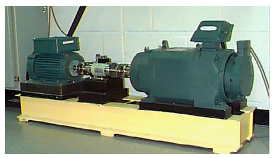
Figure 1.
Experimental device.
The experimental device includes a 2 HP (1.5 kW) motor, a torque sensor, a power meter, and an electronic controller. The load of the motor is zero. During the rotation of the motor, the bearing to be tested supports the rotating shaft of the motor. The bearing at the driving end of the rotating shaft is 6205 deep groove ball bearing, which is the bearing researched in this paper.
The single-point damage was machined on the outer ring of the bearing by EDM (Electrical Discharge Machining), and single-point damage of four different diameters, 0.007 inches, 0.014 inches, 0.021 inches, and 0.028 inches, respectively, were machined. The accelerometer, which was fixed at the rotating shaft of the motor, was used to collect the vibration signal of the fault bearing. The sampling frequency was 12 kHz. In order to get more sample data for evaluate the artificial neural network, the sampling time was 20 s for the normal bearing and 10 s for the fault bearings. The former collected 240,000 data points and the latter 120,000 data points. This paper uses data of 10 s.
3.2. Feature Extraction Method
According to the bearing experimental conditions, the bearing outer ring is fixed, the speed is 0; the speed of the bearing inner ring is 10,776 deg/s = 29.93 r/s. According to the speed relationship, the speed of the bearing cage is 4271.2 deg/s = 11.87 r/s; the angular speed of the roller is 24,971.8 deg/s = 69.37 r/s. When processing the data, the data points collected by each fault bearing need to be segmented, and the features are extracted from each segment to obtain a trained sample. In order to ensure that each section of the data points can contain a number of complete cycles of the bearing operation, take the cage that has the slowest speed as a benchmark, and ensure the cage can rotate to three laps or more when segmenting the data.
By calculating 12 kHz ÷ 11.87 r/s = 3033, so that each segment of data needs to contain at least 3033 data points in order to facilitate the calculation, this paper takes 4000 data points per segment. Using this as a standard, each of the four faulty bearings, each of which has 120,000 data points, can be divided into 30 segments, which makes 30 samples. The 240,000 data points collected on the normal bearing, in order to maintain the alignment of the samples, are also segmented to obtain 30 samples by using only the first 120,000 data points. This gives a total of 150 samples in five different fault categories. The statistical features are extracted from the acceleration signal. Equations (1)–(6) are the statistical characteristics of the formula:
(1) Mean
The mean represents the mathematical expectation of the signal, as shown in Equation (1):
(2) Root mean square (RMS)
The RMS is a measure of the size of an important indicator of vibration. From the energy point of view, it is to convert the alternating current (AC) component into the equivalent direct current (DC) component, as shown in Equation (2):
(3) Square root amplitude
The physical meaning of the square root amplitude is to reflect the vibration amplitude at a certain frequency, and the expression is as shown in Equation (3):
(4) Skewness
The skewness reflects the asymmetry of the probability density function of the signal distribution with respect to the ordinate, and the larger the skewness value is, the more serious the asymmetry is. This feature calculates the third-order central moment of the sample space, as shown in Equation (4):
(5) Kurtosis
The kurtosis is mainly effective in analyzing whether the signal contains a pulse fault. The expression is as shown in Equation (5):
(6) Standard deviation
The standard deviation, as a measure of the uncertainty of a sample, reflects the degree of dispersion of the mean of the sample data, as shown in Equation (6):
(7) Absolute mean
The absolute mean of the signal represents the statistical mathematical expectations of the absolute value, as shown in Equation (7):
The above is the dimension of statistical features. In order to ensure the consistency of the sample features, this paper also uses the dimensionless features. The calculation formulas of dimensionless features are shown in Table 1.

Table 1.
Dimensionless features.
In this paper, the above six dimensionless features are taken, besides an absolute average (dimension features), so a total of seven features are used as the input features of the training samples of the degenerative model. This paper sets normal bearings to Category 0 as a label for this category; bearings with 0.007 inches of failure are set to Category 1; bearings with 0.014 inches of failure are set to Category 2; bearings with 0.021 inches of failure are set to Category 3; bearing with 0.028 inches is set to Category 4. The label setting result is shown in Table 2.

Table 2.
Bearing labels.
Table 3 shows the results for the statistical features from each category. Here, the first three of 30 samples in each category are illustrated.

Table 3.
Value of statistical features.
3.3. The Trend of Feature Change
The features of the first 50 samples are plotted in Figure 2, Figure 3, Figure 4, Figure 5, Figure 6, Figure 7 and Figure 8.
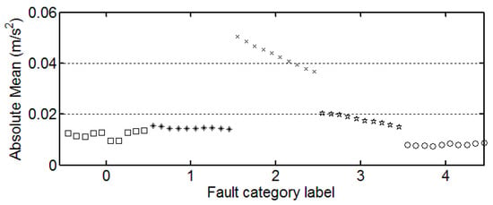
Figure 2.
The trend of absolute mean.
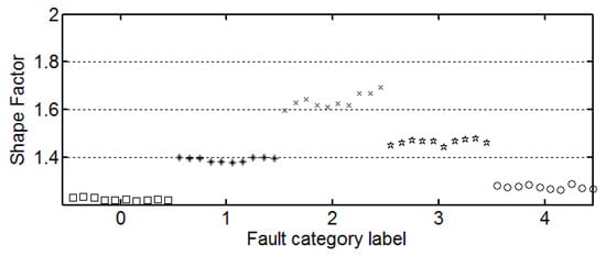
Figure 3.
The trend of shape factor.
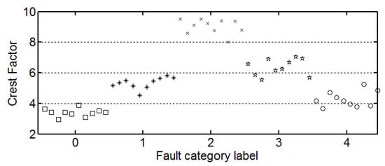
Figure 4.
The trend of crest factor.
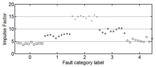
Figure 5.
The trend of impulse factor.
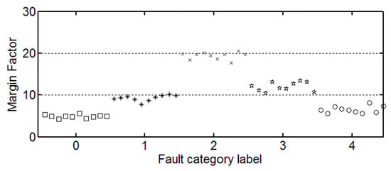
Figure 6.
The trend of margin factor.
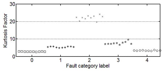
Figure 7.
The trend of kurtosis factor.
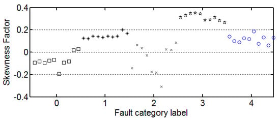
Figure 8.
The trend of skewness factor.
It can be seen from these figures that except for the sample labeled 2 (bearings with 0.014 inch fault), a single index cannot distinguish the bearing samples with different fault degrees well. The samples with different labels have a confusion in the value of feature and do not have a good distinction. Taking the trend of the kurtosis factor (Figure 7) as an example, the kurtosis factor of a normal bearing (label 0) and the kurtosis factor of a bearing with 0.028 inch fault (label 4) are basically in the same range. It is difficult to distinguish between the two categories by this feature. Therefore, the neural network degradation model is proposed based on multiple features of samples to identify and classify faults.
4. Model Training
4.1. Training Sample Division
In order to research the change of the learning process of the degenerative model with the increase of the number of samples, five different numbers of training samples are used to train the degenerative model, and the numbers are 50, 75, 100, 125, and 150. In addition, the training samples need to be divided into training sets and verification sets. The former is used to train the degradation model and the latter is used to test the degradation model. This paper takes 80% of the training data as the training set and the remaining 20% as the verification set. The division of training set and verification set is shown in Table 4.

Table 4.
Training set and verification set division.
4.2. Neural Network Degradation Model Modeling
This paper uses Python to build a neural network model, as shown in Figure 9.
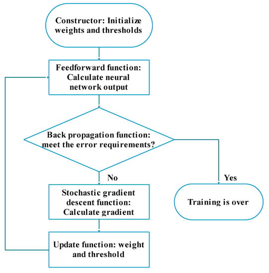
Figure 9.
Neural network model training flow chart.
The functions of the model are as follows:
(1) Constructor
The function of the constructor is to initialize the neural network, including the neural network size that needs to be set manually, and the weights and thresholds. In this paper, 0–1 Gaussian distribution (i.e., the normal distribution) is used to initialize the thresholds and weights. This method takes into account the statistical assumption of the machine learning algorithm that all the samples are independent of each other, and in the case of enough samples, the distribution of samples follows the Gaussian distribution. This assumption is based on the central limit theorem.
(2) Feedforward function
The feedforward function is to input the value to be stimulated into the excitation function to calculate the stimulus value and transmit the activation information to the next neuron.
(3) Back propagation function
The back propagation function is to calculate the error between the output of the neural network and the label of the training sample at the current weights and thresholds and inversely propagate the error as the return value to the previous neuron. This function is called the update function.
(4) Stochastic gradient descent function
The stochastic gradient descent function is the core function of training neural network. In this paper, the small batch random gradient descent method is used. Compared with the general full gradient descent method and the stochastic gradient descent method, the gradient descent method has the following advantages:
- (a)
- Compared with the full gradient descent method, the proposed method disrupts the training samples randomly while updating iteration. The training samples are divided into multiple small samples of appropriate size, and a gradient descent is used for each small sample instead of all samples. The benefit of doing so is a great reduction in the convergence time and an improvement of the calculation speed.
- (b)
- The general stochastic gradient descent method is randomly applied by a sample from the training samples while updating the iteration. Although this method can increase the calculation speed, it is easy to cause large errors. On the contrary, the small-scale stochastic gradient descent method used in this paper reduces the error while preserving the computational speed.
(5) Update function
The function of the update function is to update the weights and thresholds of the entire neural network according to the calculated gradient after applying the gradient descent to each small sample. The function is called a stochastic gradient descent function.
4.3. Model Setting
Neural network model parameters are: iteration times, small batch size of the sample, the size of the neural network, learning rate, etc.
(1) Iteration times
For ease of comparison, the neural network learning process under different sample numbers of training samples all has 1000 iteration times.
(2) Small batch size of the sample
Since there are five sample categories, the small batch sample is set to 5, which should guarantee that all classes of samples will have a high probability of occurrence each time the gradient is applied with a uniform probability.
(3) The size of neural network
For the size of the neural network, it is known that there are seven neurons (seven features) in the input layer, five neurons in the output layer (five bearings with different degrees of failure). As the number of hidden neurons in a neural network increases, the learning performance of a neural network is better, but the computation speed of the neural network is slower. In this paper, a benchmark is given when all the verification sample samples can be correctly classified after 1000 iterations. There are 50 training samples to test the minimum number of neurons needed for the hidden layer of the neural network. At the time of testing, the undetermined initial learning rate was set to 1. Hidden layer neuron number adjustment process is shown in Table 5. Here the accuracy of classification achieves 100% for 30 or 40 number of neurons. As the accuracy of classification is only the basic feature, we can make future analysis in the following sections. If we cannot get enough sampling data on faulty and healthy systems as in this experiment, indicators such as sensitivity, specificity and ROC (receiver operating characteristic) curve may be selected for the actual data.

Table 5.
Number of hidden layer neurons.
So the size of the neural network is set to 7 × 30 × 5.
(4) Learning rate
The larger the learning rate, the faster the model converges. However, if the rate is too high, the model will oscillate. Therefore, it is necessary to set the learning rate as high as possible without causing any vibration. The learning rate test was performed in the case of 50 training samples, as shown in Table 6.

Table 6.
Adjust the learning rate.
So the learning rate is set to 1.4. In summary, the initial settings of neural network model parameters are shown in Table 7.

Table 7.
Neural network model initialization parameters.
4.4. Analysis of Training Results Model Setting
The training samples of different capacities are input into the neural network training in turn, and the neural network classification results of the current weights and thresholds are calculated for each iteration. So we can observe the progress of learning accompanied by neural network classification ability. The training process is shown in Figure 10, Figure 11, Figure 12, Figure 13 and Figure 14.
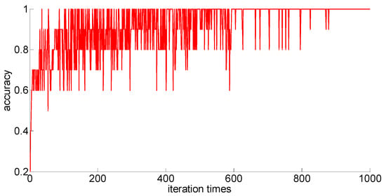
Figure 10.
Fifty training samples of the neural network.
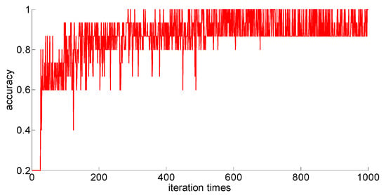
Figure 11.
Seventy-five training samples of the neural network.
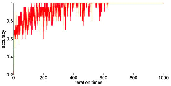
Figure 12.
One hundred training samples of the neural network.
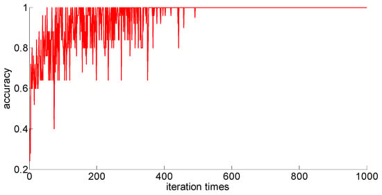
Figure 13.
One hundred twenty-five training samples of the neural network.
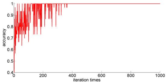
Figure 14.
One hundred fifty training samples of the neural network.
Through preliminary observation of the training process after each training sample is input into the neural network, we can see that as the number of samples increases, the classification ability of the neural network increases. At the same time, we notice that when the training sample size is 75, the training process is rather special. As the number of iterations increases, the classification accuracy of the model for the verification set does not stabilize after reaching 100%, but is 86.7% (13/15), 93.3% (14/15), and 100% (15/15). That is, oscillations occurred. In order to make a better comparison, we use some indexes to calculate them. The indexes include: the average correct classification rate of 1000 iterations, the standard deviation of the correct classification rate of 1000 iterations, the minimum iterations times and the training time required to achieve the 100% classification accuracy and maintain the stability. The calculation results are shown in Table 8.

Table 8.
Training outcome indicators for different training sample sizes.
Since different sample size models converge in different iterations, the corresponding iterations are set according to the training results for the training under each sample size to test the training time. The results are shown in Table 9.

Table 9.
Convergence training time test.
From the above results, we can make the following observations.
- (1)
- In addition to the sample size of 75, with the increase of training sample size, the learning effect of the neural network will get better and better. The average correct rate of classification under the setting of 1000 iterations, the standard deviation of classification accuracy, the minimum number of iterations, the training time, and other indicators showed an increasing trend, indicating that the learning ability of the model, the learning stability, and the convergence rate of the calculation will increase with the increase in training samples.
- (2)
- When the sample size is 75, the model oscillates during the training process. When the training sample size increases, the phenomenon vanishes. It can be seen that it is not because the learning rate is set improperly. Instead, there are some indistinguishable sample points and we should enhance the learning ability and generalization ability of the model to increase the training samples. This is confirmed by the test results after increasing the sample size.
5. Feature Fusion Based on Skewness Factor
Based on the above study, it can be seen that even with 150 samples (the largest number of samples), the BP neural network model still needs 365 iterations to converge smoothly so as to obtain 100% correct classification of the verification set, and the calculation time required is 11.43 s. As offline calculation of the script, this calculation time is completely acceptable, but to apply the model to online monitoring procedures for real-time updates on the model, the calculation speed needs to be improved.
Based on the sigmoid function activation function, which turns linear regression into a classification problem in order to improve the fitting ability of the neural network, we need to improve the nonlinearity of variables in linear regression. This paper starts with a study of adding nonlinear fusion features.
5.1. Pearson Correlation Coefficient between Features
In order to research the change of the learning process of the degenerative model with an increase in the number of samples, five different numbers of training samples are used to train the degenerative model: 50, 75, 100, 125, and 150. In addition, the training samples need to be divided into training sets and verification sets. The former are used to train the degradation model and the latter are used to test the degradation model. This paper takes 80% of the training data as the training set and the remaining 20% as the verification set. The division of training set and verification set is shown in Table 5.
The Pearson correlation coefficient is a linear correlation coefficient that reflects the linear correlation between two variables, the value of which is between −1 and 1. The smaller the absolute value, the lower the correlation. Supposing two variables x and y, each having n samples, correspond to n values, the formula for calculating the Pearson correlation coefficient r between x and y is shown in Equation (8):
For all 150 training samples, the Pearson correlation coefficients between the two features are calculated. The calculation results are shown in Table 10.

Table 10.
Pearson correlation coefficients between features.
According to the results, it can be seen that the Pearson correlation coefficient between the skewness factor and other features is significantly lower than the Pearson correlation coefficient between the other features. The skewness factor has a strong nonlinear relationship with other features. Therefore, we choose the skewness factor for the feature fusion.
5.2. Feature Fusion Pearson
In order to research the change of the learning process of the degenerative model with the increase of the number of samples, five different numbers of training samples are used to train the degenerative model: 50, 75, 100, 125, and 150. In addition, the training samples need to be divided into training sets and verification sets. The former are used to train the degradation model and the latter are used to test the degradation model. This paper takes 80% of the training data as the training set and the remaining 20% as the verification set. The division of training set and verification set is shown in Table 5.
When the relationship between two variables is non-linear, in order to better fit the variables, it is usually considered to use quadratic polynomials or even higher-degree polynomials to fit. The general form of quadratic polynomial fitting is shown in Equation (9):
Among them, , , and xy increase the fitting nonlinearity, making the quadratic polynomial fit the general linear regression with a more complex curve. Inspired by this, and considering the use of skewness factor with very low Pearson coefficients with all features to multiply other features, six new fusion features are constructed. The absolute value of the Pearson correlation coefficient between the skewness factor and the fused features is sorted accordingly. The results are shown in Table 11.

Table 11.
New features based on skewness factor fusion.
Considering that too many features will lead to an overfitting of the model, based on the training samples of 50 samples, we gradually add features to the sample from the new feature 1 until the model is overfitting, and the result is shown in Table 12. The experimental results show that when the number of features increases to three, the model begins to overfitting. Therefore, two new features are added based on the original features of the sample: new feature 1 and new feature 2.

Table 12.
Test result of new features with 50 samples.
5.3. New Feature Verification
After adding new feature 1 and new feature 2 based on the original features of the sample, in order to compare with the original neural network model, the other parameters of the neural network model are kept unchanged; only the size of the neural network is changed from 7 × 30 × 5 to 9 × 30 *× 5. Then training samples with different capacities are input into the neural network training in turn; the training process is shown in Figure 15, Figure 16, Figure 17, Figure 18 and Figure 19.
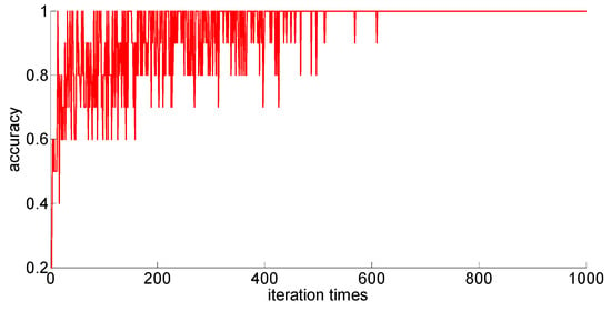
Figure 15.
Fifty training samples of the neural network.
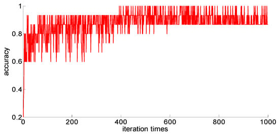
Figure 16.
Seventy-five training samples of the neural network.
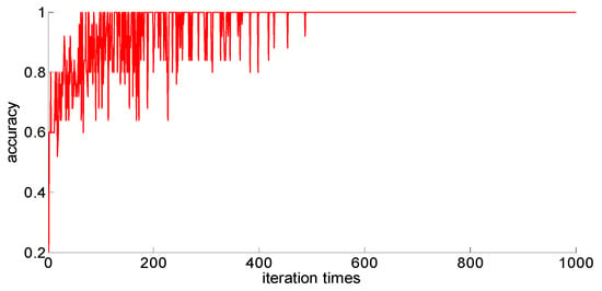
Figure 17.
One hundred training samples of the neural network.
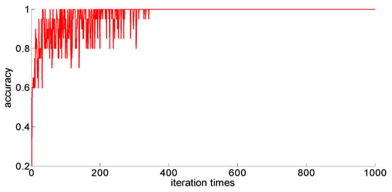
Figure 18.
One hundred twenty-five training samples of the neural network.
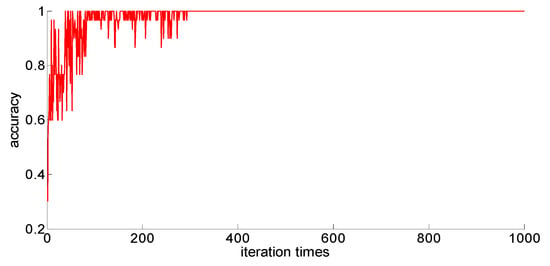
Figure 19.
One hundred fifty training samples of the neural network.
After completing the training, four indexes for evaluating the training effect are counted, and the training effect of the model after adding the new feature is compared with the training effect of the previous model. The results are shown in Table 13. Similarly, the number of iterations for different sample size models to converge is also different, and the corresponding iterations are set according to the training results for the training under each sample size to test the training time. The results are shown in Table 14.

Table 13.
Different training sample size model training results indicators comparison.

Table 14.
Comparison of model training results with different number of training samples.
After a comparison, we can draw the following conclusions:
- (1)
- Compared with the previous model, the model with new features 1 (skewness × shape) and new features 2 (skewness × crest) has been obviously improved in the training effect, and the average accuracy of the classification has improved too. The standard deviation of classification accuracy, the least number of iterations, training time, and so on all improved, which shows that adding new features can improve the model’s learning ability, learning stability, and the convergence rate of the calculation.
- (2)
- After adding new features, the training sample size is 75; although these three indicators, the classification accuracy, the standard classification accuracy, and the minimum number of iterations, are all improved, the oscillation phenomenon still exists. If you want to further improve the model’s ability to classify difficult-to-distinguish sample points, you need to increase your training sample size.
It should be noted that the decision to add only two new features was based on a training sample size of 50 benchmark results. With the increase in the sample size, the ability of the model to prevent overfitting is constantly improving. So, we use a training sample size of 150 to test what happens when the sample size increases, and continuing to add new features will not further enhance the effectiveness of the model. When the model appears to be overfitting, we will get the stop condition, as shown in Table 15.

Table 15.
Test results of new features with 150 samples.
When the number of new features is increased to three, the effect of the model is further improved. When the number of new features is increased to more than four, the model appears to be overfitting again. Thus, as the capacity of the training samples increases, new fusion features continue to be added to further enhance the effect of the model. Even when no more data are being collected, we can continue to increase the new fusion features to improve the neural network algorithm to establish the effect of the bearing degradation model.
5.4. Comparison with SVM
In this section, the result of neural network is compared with SVM, as shown in Table 16. The main indicators for the verification are the classification accuracy and the training time.

Table 16.
Results comparison between neural network and SVM.
- (1)
- For the classification ability, the degenerative model built by neural network or SVM has the same effect. Even in the case of 75 training samples, the classification accuracy of the degraded model built by SVM is also in the oscillation range of neural network.
- (2)
- The training time of the degenerative model built by neural network is actually longer than the model by SVM. It can be seen that SVM is the better model than neural network for the 6205 bearing.
- (3)
- Although the performance of neural network is weaker than that of SVM, it should be noted that for neural network, with an increase in the number of training samples and the inclusion of fusion features, the improvement of training speed is obvious. In contrast, for SVM, with an increase in the number of training samples, although the computational speed of each iteration increases, the total training time is not significantly reduced. The training time ratio of SVM and neural network has increased from 11.57% in 50 training samples to 16.41% in 150 training samples.
6. Conclusions
This paper uses a BP neural network algorithm to build a degradation model of 6205 deep groove ball bearings, through the degradation model to identify and classify the different fault state of the bearing. The main research results are as follows:
- (1)
- In this paper, 150 training samples were extracted from the experimental data collected in the experiment, and five training samples of 50, 75, 100, 125, and 150 samples were extracted from the training data and input into the neural network for training. The training results show that with an increase in training sample size, the learning effect of the neural network gets better and better, and the learning ability, learning stability, and convergence speed of the model gradually increase.
- (2)
- When the training sample size is 75, with an increase in the number of iterations, the classification accuracy of the model to the verification set fails to stabilize at 100%, resulting in oscillation. When the number of samples increases, the oscillation phenomenon disappears. It can be seen that the oscillation occurs not because the model itself, but the indistinguishable samples. The results show that further enhancement of the classification ability of BP neural network degeneration model for indistinguishable samples needs to be achieved by increasing the training sample size.
- (3)
- Based on the Pearson correlation coefficient and polynomial fitting principle, feature fusion based on the skewness factor improves the model significantly. Although too many fusion features lead to overfitting of the model, overfitting will be alleviated with the increase in training samples. The model’s performance can be further improved by increasing the fusion features.
- (4)
- The comparison of the performance of the SVM model and the neural network model on this dataset is discussed, and the possible effects and performance of these two different modeling methods on more complicated problems and more data are discussed. The research shows that neural networks have more potential on complex and high-volume datasets.
Acknowledgments
This work was financially supported by the National Key Research and Development Program of China (No. 2016YFF0203804), the National Natural Science Foundation of China (No. 51775037), and the Fundamental Research Funds for Central Universities of China (No. FRF-TP-15-010A3).
Author Contributions
Lijun Zhang and Junyu Tao conceived and designed the experiments; Junyu Tao performed the experiments and analyzed the data; Lijun Zhang and Junyu Tao wrote the paper.
Conflicts of Interest
The authors declare no conflict of interest.
References
- Huang, Y. Advances in artificial neural networks—Methodological development and application. Algorithms 2009, 2, 973–1007. [Google Scholar] [CrossRef]
- Rai, A.; Upadhyay, S.H. The use of MD-CUMSUM and NARX neural network for anticipating the remaining useful life of bearings. Measurement 2017, 111, 397–410. [Google Scholar] [CrossRef]
- Dubey, R.; Agrawal, D. Bearing fault classification using ANN-based Hilbert footprint analysis. IET Sci. Meas. Technol. 2015, 9, 1016–1022. [Google Scholar] [CrossRef]
- Li, S.; Liu, G.; Tang, X.; Lu, J.; Hu, J. An ensemble deep convolutional neural network model with improved DS evidence fusion for bearing fault diagnosis. Sensors 2017, 17, 1729. [Google Scholar] [CrossRef] [PubMed]
- Sadegh, H.; Mehdi, A.N.; Mehdi, A. Classification of acoustic emission signals generated from journal bearing at different lubrication conditions based on wavelet analysis in combination with artificial neural network and genetic algorithm. Tribol. Int. 2016, 95, 426–434. [Google Scholar] [CrossRef]
- Meng, Z.; Hu, M.; Gu, W.; Zhao, D. Rolling bearing fault diagnosis method based on LMD multi scale entropy and probabilistic neural network. China Mech. Eng. 2016, 27, 433–437. [Google Scholar] [CrossRef]
- Prajapati, D.K.; Tiwari, M. Use of artificial neural network (ANN) to determining surface parameters, frictionand wear during Pin-on-Disc tribotesting. Key Eng. Mater. 2017, 739, 87–95. [Google Scholar] [CrossRef]
- Zhao, N.; Zheng, H.; Yang, L.; Wang, Z. A fault diagnosis approach for rolling element bearing based on S-Transform and artificial neural network. In Proceedings of the ASME Turbo Expo 2017: Turbomachinery Technical Conference and Exposition, Charlotte, NC, USA, 26–30 June 2017; Volume 6. [Google Scholar] [CrossRef]
- Karkan, P.K.; Satish, C.S.; Harsha, S.P. Fault diagnosis of ball bearings using machine learning methods. Exp. Syst. Appl. 2011, 38, 1876–1886. [Google Scholar] [CrossRef]
- You, W.; Shen, C.; Guo, X.; Jiang, X.; Shi, J.; Zhu, Z. A hybrid technique based on convolutional neural network and support vector regression for intelligent diagnosis of rotating machinery. Adv. Mech. Eng. 2017, 9, 116–134. [Google Scholar] [CrossRef]
- Jia, F.; Lei, Y.; Lin, J.; Zhou, X.; Lu, N. Deep neural networks: A promising tool for fault characteristic mining and intelligent diagnosis of rotating machinery with massive data. Mech. Syst. Signal Process. 2016, 72, 303–315. [Google Scholar] [CrossRef]
- Zhang, W.; Li, C.; Peng, G.; Chen, Y.; Zhang, Z. A deep convolutional neural network with new training methods for bearing fault diagnosis under noisy environment and different working load. Mech. Syst. Signal Process. 2018, 100, 439–453. [Google Scholar] [CrossRef]
- Wang, F.; Jiang, H.; Shao, H.; Duan, W.; Wu, S. An adaptive deep convolutional neural network for rolling bearing fault diagnosis. Meas. Sci. Technol. 2017, 28, 223–237. [Google Scholar] [CrossRef]
- Jiang, H.; Wang, F.; Shao, H.; Zhang, H. Rolling bearing fault identification using multilayer deep learning convolutional neural network. J. Vibroeng. 2017, 19, 99–104. [Google Scholar] [CrossRef]
- Lu, C.; Wang, Z.; Zhou, B. Intelligent fault diagnosis of rolling bearing using hierarchical convolutional network based health state classification. Adv. Eng. Inf. 2017, 32, 39–151. [Google Scholar] [CrossRef]
- Chen, Z.; Deng, S.; Chen, X.; Li, C.; Sanchez, R.-V.; Qin, X. Deep neural networks-based rolling bearing fault diagnosis. Microelectron. Reliab. 2017, 75, 327–333. [Google Scholar] [CrossRef]
- He, J.; Yang, S.; Gan, C. Unsupervised fault diagnosis of a gear transmission chain using a deep belief network. Sensors 2017, 17, 1564. [Google Scholar] [CrossRef] [PubMed]
- Eren, L. Bearing fault detection by one-dimensional convolutional neural networks. Math. Probl. Eng. 2017, 8, 146–154. [Google Scholar] [CrossRef]
- Kanai, R.A.; Desavale, R.G.; Chavan, S.P. Experimental-based fault diagnosis of rolling bearings using artificial neural network. J. Tribol. 2016, 138, 31–53. [Google Scholar] [CrossRef]
- Yang, D.; Mu, H.; Xu, Z.; Wang, Z.; Yi, C.; Liu, C. Based on soft competition ART neural network ensemble and its application to the fault diagnosis of bearing. Math. Probl. Eng. 2017, 17, 112–119. [Google Scholar] [CrossRef]
- Jiang, P.; Hu, Z.; Liu, J.; Yu, S.; Wu, F. Fault diagnosis based on chemical sensor data with an active deep neural network. Sensors 2016, 16, 169–185. [Google Scholar] [CrossRef] [PubMed]
- Gan, M.; Wang, C. Construction of hierarchical diagnosis network based on deep learning and its application in the fault pattern recognition of rolling element bearings. Mech. Syst. Signal Process. 2016, 72, 92–104. [Google Scholar] [CrossRef]
- Zhao, Z.; Xu, Q.; Jia, M. Improved shuffled frog leaping algorithm-based BP neural network and its application in bearing early fault diagnosis. Neural Comput. Appl. 2016, 27, 375–385. [Google Scholar] [CrossRef]
- Smith, W.A.; Randall, R.B. Rolling element bearing diagnostics using the Case Western Reserve University data: A benchmark study. Mech. Syst. Signal Process. 2015, 64–65, 100–131. [Google Scholar] [CrossRef]
© 2018 by the authors. Licensee MDPI, Basel, Switzerland. This article is an open access article distributed under the terms and conditions of the Creative Commons Attribution (CC BY) license (http://creativecommons.org/licenses/by/4.0/).