Abstract
This paper addresses a modeling and analysis methodology for investigating the stochastic harmonics and resonance concerns of wind power plants (WPPs). Wideband harmonics from modern wind turbines (WTs) are observed to be stochastic, associated with real power production, and they may adversely interact with the grid impedance and cause unexpected harmonic resonance, if not comprehensively addressed in the planning and commissioning of the WPPs. These issues should become more critical as wind penetration levels increase. We thus propose a planning study framework comprising the following functional steps: First, the best fitted probability density functions (PDFs) of the harmonic components of interest in the frequency domain are determined. In operations planning, maximum likelihood estimations (MLEs) followed by a chi-square test are used once field measurements or manufacturers’ data are available. Second, harmonic currents from the WPP are represented by randomly-generating harmonic components based on their PDFs (frequency spectrum) and then synthesized for time domain simulations via inverse Fourier transform. Finally, we conduct a comprehensive assessment by including the impacts of feeder configurations, harmonic filters and the variability of parameters. We demonstrate the efficacy of the proposed study approach for a 100-MW offshore WPP consisting of 20 units of 5-MW full converter turbines, a realistic benchmark system adapted from a WPP under development in Korea and discuss lessons learned through this research.
1. Introduction
Integrating high penetrations of variable renewable sources into the electric power grid presents a range of unprecedented grid operations and planning challenges requiring new study approaches and tools so that the impacts of a proposed wind power plant (WPP) can be properly assessed prior to interconnection [1,2,3,4,5]. In particular, increasing attention has been drawn to power quality concerns: harmonics and the output harmonic impedance of wind turbines (WTs) and the aggregating WPP are stochastic due to the inherent intermittency of the wind and wide control bandwidth of the power electronics interfaces [6,7]. These wideband stochastic harmonic emissions from modern converter-based WTs may adversely interact with the grid via vast underground or submarine cable systems, leading to many series and parallel resonance points that significantly change with the harmonic filters, feeder configuration and reactive power compensation devices associated with the number of WTs in operation [1,7,8,9].
Probabilistic aspects of harmonics in electric power systems especially due to dynamic nonlinear loads have long been observed, and numerous research efforts suggest that statistical representations and analyses of time-varying harmonics are desired and present methods for determining the statistical distributions of harmonics and limits [10,11,12,13,14]. However, little effort for representing harmonic characteristics of the renewable generation has been exerted in system planning studies. Recent analyses of harmonic emissions from WTs by type interestingly claim that we may statistically characterize harmonic components with certain probabilistic distributions independent of the wind power generation (i.e., operating condition) in contrast with the fundamental current, which should be proportional to the wind power [7,8,15]. Resonance concerns in line with these harmonics arise when one of the harmonics coincides with the resonance frequency. It is well understood that the resonance points vary with changes in the system operating conditions; for example, the number of operating WTs due to wind maintenance or failure and the operation of filters and switched shunts [1,16,17]. An IEEE working group collaboratively investigated these harmonics and resonance issues within a WPP and summarized the compliance, mitigation measures and analysis methods, such as the harmonic impedance scan [18]. It is interesting to note the efforts to identify the spectral characteristics of the WPP by aggregating those of WTs [19,20].
Although harmonics and resonance issues have been investigated and well reported as above, the grid planners are increasingly challenged due to the lack of a comprehensive and practical planning study process and supporting tools, to the extent of authors’ knowledge and experience. They still rely on deterministic analysis often based on the worst case scenarios without effectively incorporating observations and knowledge gained through extensive efforts recently [19,20]. The study scope and results could thus be limited and possibly lead to unnecessary capital investment. Pursuing comprehensiveness, flexibility and practicality for implementing a supporting tool of the approach, this research proposes a statistical modeling and planning study methodology for investigating the stochastic harmonics and resonance concerns of WPPs. We observe that existing methods, such as random harmonic phasor summation [21] or harmonic summation introduced in the standard IEC 61400-21, are unable to fully capture the harmonic behavior of modern WPPs, and the results from both methods could be misleading [22,23,24]. By incorporating the statistical distribution of each harmonic component of interest from WTs and representing the overall time-varying harmonic behavior of WPPs, system planners can synthesize credible operating scenarios and investigate and collectively quantify harmonics and resonance concerns. The deterministic approach or its variation by incorporating certain correlations in the generators, for example operating closely, can also be taken in this proposed framework for comparison. System operators can exploit both stochastic and deterministic approaches, as well, to investigate unforeseen problematic operating conditions and, thus, systematically develop mitigation or correction measures. The proposed modeling and analysis framework is presented in Figure 1 and will be elaborated in the paper.
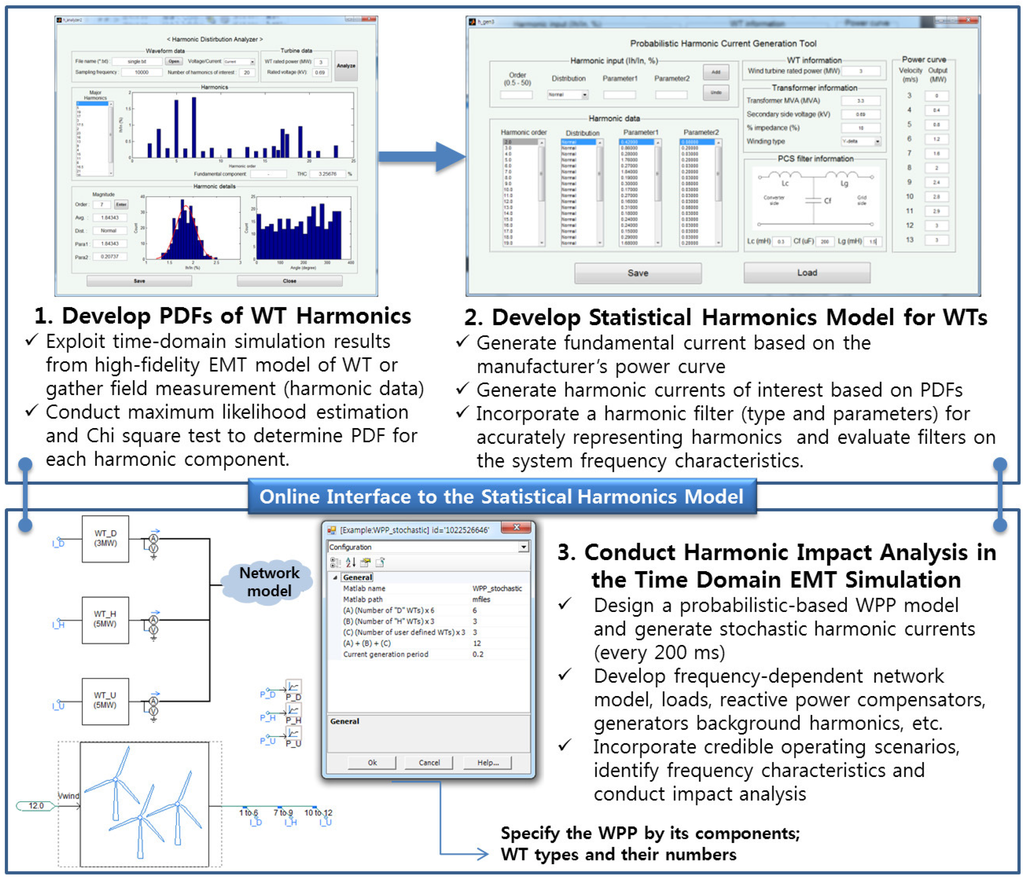
Figure 1.
Proposed study framework and its implementation using MATLAB and PSCAD/EMTDC for assessing stochastic wind harmonics. PDFs: probability density functions; WT: wind turbine; EMT: electromagnetic transients; WPP: wind power plant.
This paper is structured as follows: Methods for statistic modeling are reviewed in Section 2. Section 3 presents a proposed method designed for generating harmonic emissions of the WTs. Next, a modeling of a WPP is presented in Section 4. Harmonics for a single turbine model are assessed in Section 5 followed by a practical harmonic evaluation for a realistic test system designed based on an offshore WPP (100 MW) under development in Korea in Section 6.
2. Statistical Modeling
As illustrated in Figure 1, the approach develops statistical models of fundamental and harmonic currents from WTs and WPPs based on prior theoretical and empirical knowledge based on actual harmonic measurements of the WTs and WPP at the point of connection (PoC), which should be the case in operations planning. In grid planning, simulation results from high-fidelity models and data from the manufacturers can be used for this purpose because field measurements are not generally available. Measurements from already operating sites may also be considered for use as long as similar WTs and operating conditions are to be adopted: the offshore WPPs under development and in planning in Korea should be the case.
To capture the statistical characteristics of each harmonic component, we then fit probability density functions (PDFs) to the experimental data and incorporate them in the model as the noted frequency domain analysis in Figure 1. The maximum likelihood estimation (MLE) and chi-square goodness-of-fit test are finally applied to determine the best fit for each harmonic component among feasible PDFs.
2.1. Maximum Likelihood Estimation
The characteristics of harmonic components are observed to be stochastic in terms of their magnitudes and locations. Proprietary converter topology and controls and various filter types should be contributing factors on top of variable wind. Well-known parametric PDFs could be fitted to each harmonic component. Custom mathematical and even nonparametric distribution functions may be investigated as needed. This research applies the MLE method to determine the parameters of the PDFs [25,26].
Let , ..., be independent, identically-distributed samples of a random variable with a PDF, , where is a vector of parameters that characterize . The joint PDF of the n samples can be obtained as shown in Equation (1):
A likelihood function is specified as shown in Equation (2), and the parameters are continuously updated until the likelihood is maximized:
The parameters are estimated by differentiating Equation (2). This process is often carried out with the logarithm of the likelihood Equation (2):
The PDF of a harmonic component is often observed to be the normal distribution as specified below [7,8,9,15]:
where is the average and is the standard deviation. Both parameters can be estimated by Equations (1) and (2), as illustrated in Figure 2.
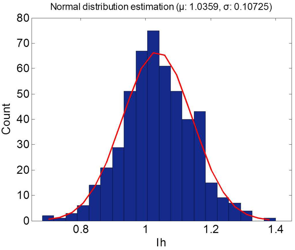
Figure 2.
Example of maximum likelihood estimation (MLE) based on the histogram data. Current measurement at a certain harmonic order takes the normal distribution for which the parameters of the average and standard deviation are estimated.
2.2. Chi Square Test
The statistical behavior of a particular harmonic component could be represented by a variety of PDFs. It is then necessary to evaluate how well the dataset matches a specific distribution and whether a dataset is consistent with different probability distributions. This research thus conducts a chi-square goodness-of-fit test to identify the PDF that most appropriately reflects the harmonic characteristics [27].
The chi-square test determines whether the estimation of the probability is suitable or not by using the error between the real value and the estimated value. If and are a real value and an expected value, respectively, the chi-squared value is defined as:
According to the degree of freedom, which is defined as , where k is the number of categories existing in the whole set, the p-value is defined with the approximate chi-squared distribution.
The p-value indicates the probability that the chi-squared distribution under a certain degree of freedom is larger than the chi-squared value obtained from Equation (5). If the p-value is less than 0.05, for example, the assumption of the probability is proven to be false.
However, it is challenging to identify PDFs that fit the measured harmonics from WTs or WPPs and pass this test. Therefore, the chi-square test can be adapted to identify the distribution with the least error: the chi-square value indicates the overall error of the distribution. Thus, the distribution with the least chi-square value can be considered as the best fit among several distributions.
3. Harmonic Current Generation
Following the steps presented in Section 2 above, we can develop mathematical models for generating harmonic currents with the desired statistical characteristics. It is worth mentioning that the magnitudes and phases of the harmonics from each WT are assumed to be statistically independent, such that harmonics from each WT comprising the WPP are generated independently as analyzed from field measurements [7,9]: This assumption may be refined as needed if actual measurements at strategic locations are available. The following subsections detail how we can exploit them in the simulation studies by determining the magnitude and phase angle of each harmonic current in the frequency domain and generating harmonic currents in the time domain simulation through inverse fast Fourier transform (FFT).
3.1. Determining the Harmonic Current Magnitudes
Each harmonic component from a WT and WPP is reportedly characterized by its own PDF [7,8,9,15], as detailed and conceptually illustrated in Section 4 (Figure 7). Some harmonics may take PDFs of the same type, but characterizing parameters should be unique. We randomly generate harmonic magnitudes based on these predetermined PDFs (this research exploited the output of a high-fidelity simulation model from a WT manufacturer due to a lack of actual measurements in the planning; see the Appendix A for the system parameters). Details about how to obtain the harmonic magnitudes are provided in the next section. We may exclude negligible harmonics and focus on dominant ones, such as low-order harmonics with high magnitudes and inter-harmonics in the switching frequency range or any other problematic components close to the resonance points. The generated random numbers, representing harmonic magnitudes, are recorded in the frequency domain. Once the corresponding phase angles are determined as detailed below, these generated magnitudes at selected harmonic orders go through inverse-FFT and feed into the time domain simulation as noted in the WPP model in Figure 1.
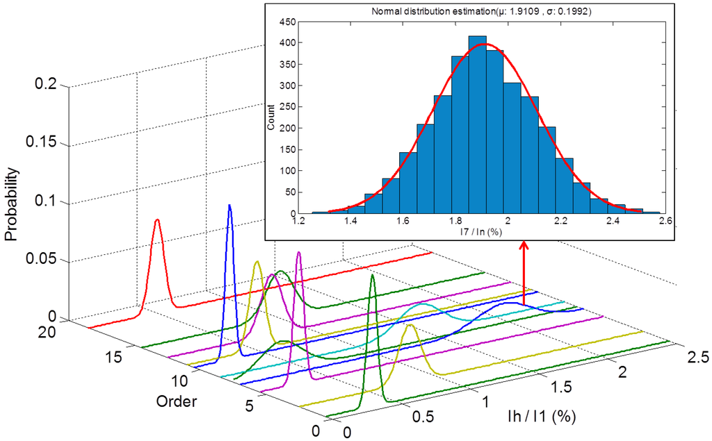
Figure 7.
Approximated PDFs of the harmonic currents from a WT and the histogram of the seventh order harmonic based on the simulation results.
3.2. Determining the Harmonic Current Phase
To perform the inverse FFT, the phase angle of each harmonic component should also be identified. In contrast to the magnitudes, the phase angles are difficult to describe with certain characteristics. As observed in [8], the phase angles of low-order harmonics tend to be synchronized to the fundamental frequency, whereas phase angles in the high-frequency range (≫1 kHz) vary randomly. A combination of normal and uniform distributions for phase angles is proposed in [7], and a uniform distribution is assumed in [19,23]. Because there is no commonly-accepted rule to define the characteristics of phase angles, this research assumes that phase angles are uniformly distributed. However, as for the magnitudes, the proposed framework flexibly allows for designing PDFs of phase angles based on the actual measurements once they are available.
3.3. Inverse Fast Fourier Transform Analysis
Before the inverse FFT is performed, the interval and range of the frequency should be decided. According to [22], FFT analysis should be extended up to the 50th-order harmonic to consider high-frequency harmonics from power electronic devices. Furthermore, in [28], the interval of 5 Hz and the sub-grouping method of harmonics, used to improve the harmonic assessment, are recommended. The sub-grouping method is used to sum adjacent harmonic components. By using the sub-grouping method, inter-harmonics with a 5-Hz frequency resolution can be simply expressed in a summation form. To reflect inter-harmonic components in a simple manner for the harmonic current generation, it is assumed that they are sub-grouped and turned into a single representative value. For instance, the nine inter-harmonics (250, 255, ..., and 290 Hz) that exist between the fourth and fifth order are summed up and replaced by a single number of 4.5.The result of the inverse FFT is a waveform of the current that includes the harmonic components for a period of time. By adjusting the interval and range in the frequency domain, it is possible to change the number of samples and the length of the waveform in the time domain.
4. Modeling a Wind Power Plant
This section focuses on modeling critical components in the planning studies of a WPP when stochastic harmonics and resonance concerns are evaluated. Models are designed to capture the effect of the power conditioning system (PCS) harmonic filter, the relationship between the operating point of the WTs and the harmonic magnitudes and the harmonics of interest.
4.1. Power Conditioning System Filter Gain and Measurement Location
In general, measurement devices obtain filtered harmonic signals for analysis. Because the analysis of harmonic resonance has become more important in WPP design and system integration, the impact of the filter on the resonance frequency should not be neglected. To revise the current source model by including the filter in the WT equivalent model, the restoration of the unfiltered signals from the filtered signal is required.
In [29], the harmonic filter gains are calculated by considering the filter impedance, transformer impedance and grid impedance. They are then multiplied by the filtered current for the restoration. This study assumes that the impedance behind the transformer is zero, and the harmonic data of the turbine are measured when the turbine is connected to an infinite bus via a transformer for the simplicity of analysis (This study relies on the detailed WT model and, thus, observes its pure harmonic contribution. When actual measurements are used, this assumption is, however, no longer valid, and the impact of grid impedance needs to be incorporated.), as depicted in Figure 3.
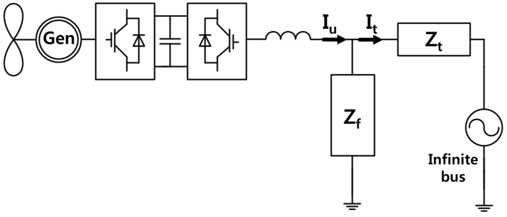
Figure 3.
Configuration of the full converter-type WT for calculating the restoration factor.
The filter type and parameters are determined based on the manufacturers’ data. In addition, the information about the phase angle should be included to restore the signal because the capacitance and inductance vary with frequency. Due to the parallel connection of the high pass filter impedance, , and the transformer impedance, , the unfiltered harmonic currents, , and the restoration factor, , are expressed as follows:
where is the current flowing through the transformer.
4.2. The Relationship Between the Wind Turbine Operating Point and the Harmonic Magnitude
The fundamental current is proportional to the power output of the WT. In contrast, there is no consensus about the relation between the WT operating point and the harmonic magnitude. In [8,9], the harmonic current magnitudes are less dependent on the operating point, which however needs to be further elaborated. When the operating point varies, different PDFs are observed in [15]. Furthermore, in [6], the individual harmonics or inter-harmonics can be either dependent on or independent of the active power production. These various cases of harmonic generation imply that the stochastic characteristics of harmonic generation are different from case to case. For simplicity, this research assumes that the distributions of the ratio of each harmonic to the rated current are independent of the operating point, as presented in [8]. However, actual data may override this assumption.
4.3. Harmonics of Interest
Stochastic analysis should carefully determine which harmonic components are included and analyzed for the harmonic effect of WPPs. Based on the measured harmonic data, harmonics that hold high magnitudes are the first to be included. Furthermore, significant inter-harmonics, in which the sub-grouping method is utilized, are considered. Because the sub-grouping method proposed in [28] uses the summation rule to concentrate nearby inter-harmonics into one representative data point, it is possible to include important inter-harmonics near the switching frequency of the PCS. In addition, harmonics in WPPs are tightly linked to the resonance problem. The resonance frequency at the PoC should be taken into consideration. By including the harmonic components near the resonance frequency, it can be determined whether or not there are resonance problems.
4.4. Single Wind Turbine Modeling
Before a practical case study is carried out, a 5-MW equivalent WT is modeled based on the manufacturer’s data. A configuration of the single turbine model is presented in Figure 4. The harmonic filter in this particular case consists of the filter reactor, filter capacitor, damping reactor and damping resistor. Transformer leakage reactance is considered as a reactor, as detailed in the Appendix A.
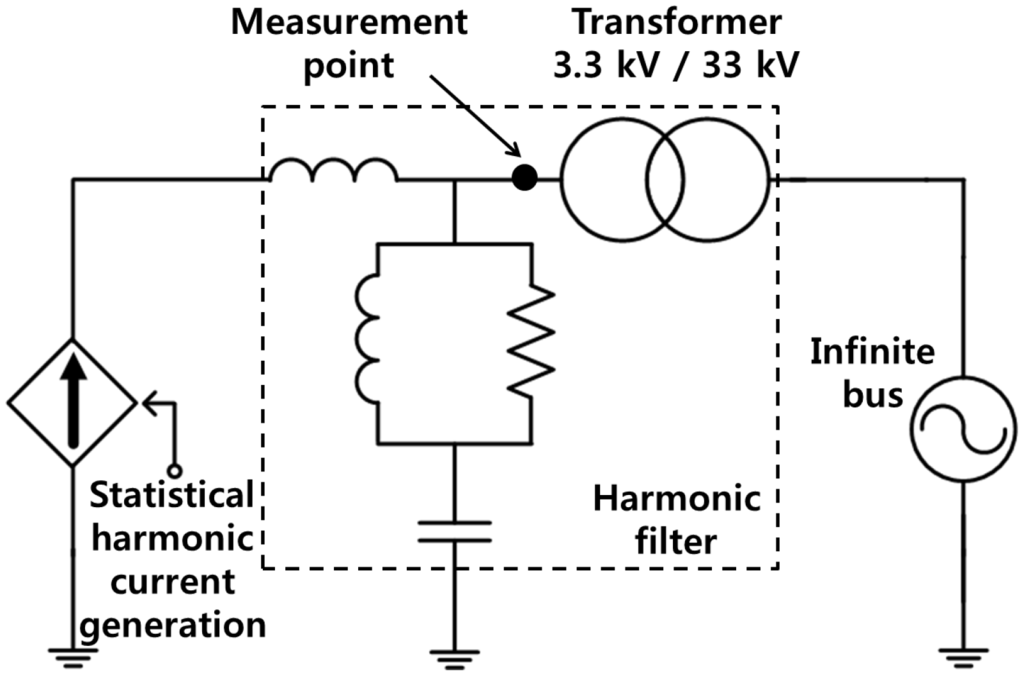
Figure 4.
Configuration of the equivalent WT model comprising the equivalent harmonic source, harmonic filter and transformer connected to the infinite bus.
The turbine is equivalently modeled as a current source with time-varying harmonic components. The filter is placed between the turbine and the transformer connected to the infinite bus without the grid impedance, as mentioned before. The magnitude and phase angle of the restoration factor in the equivalent circuit with respect to the harmonic order are shown in Figure 5. The magnitude of the restoration factor has its minimum value at the eight order and increases as the harmonic order increases. The phase of the restoration factor also shows a steep rise at the eighth order. These indicate that the circuit shown in Figure 3 has a resonance point at the eighth order, and the harmonic components near the eighth order may become prominent. Figure 5 also indicates that the higher order harmonics can be suppressed. The magnitude of every harmonic component is assumed to follow the normal distribution. The standard deviation of each harmonic component is set to 10% of its average value, and the phase is uniformly distributed in the range from 0 to . The WT is simulated to deliver 100% of its rated power for 10 min. Figure 6 compares the measured current harmonic data from a manufacturer to the 10-minute-averaged simulation data.
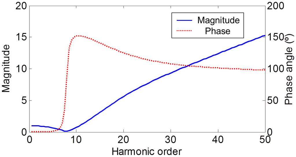
Figure 5.
Magnitude and phase of the restoration factor of the equivalent WT model with respect to the harmonic order.
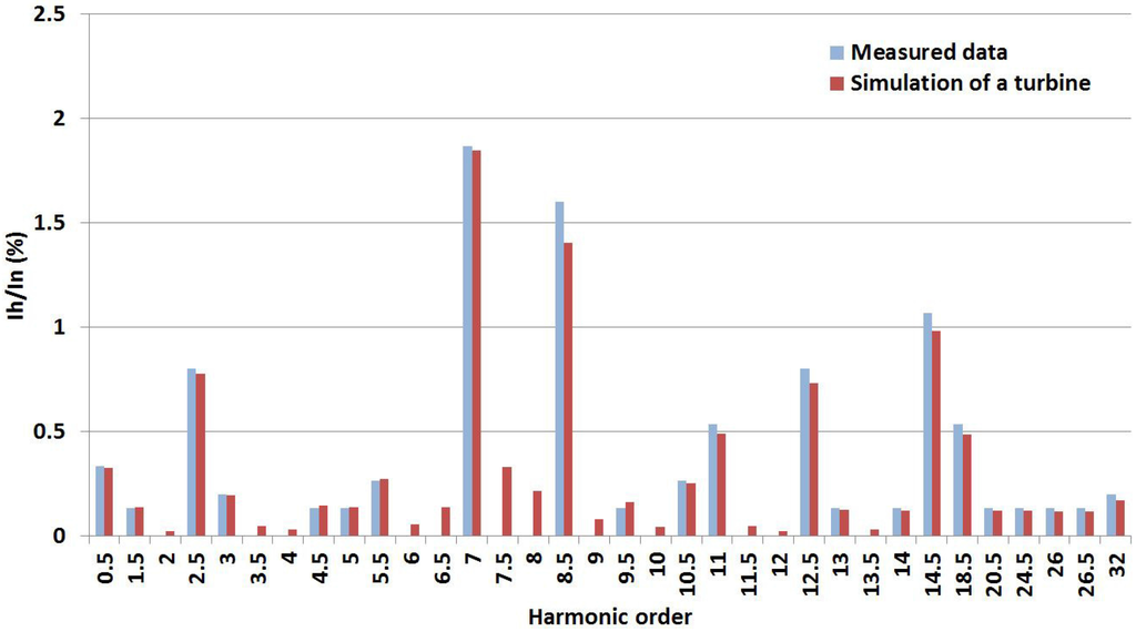
Figure 6.
Comparison between the measured data and the simulation result of the single turbine.
The measured data include the harmonics of interest, such as the harmonics in the range of the resonance frequency and the inter-harmonics near the switching frequency. Other negligible harmonic components are truncated to be zero. Although few unexpected negligible harmonics are revealed in the simulation (6.5th, 7.5th and 8th), the tendency of the harmonic generation of the turbine is closely reproduced. Due to the interaction between the filter impedance and harmonic components (discussed in Section 4), the seventh-order and 8.5th-order harmonics are two largest harmonic components generated by the turbine. The 14.5th harmonic component is also a significant harmonic component that is a sideband harmonic of the switching frequency. Figure 7 illustrates harmonic PDFs, which are approximated by the MLE on the detailed simulation results.
Figure 7 presents that the proposed model produces stochastic harmonic components following specific PDFs with their unique parameters, such as seventh-order harmonic from the simulation results, which features the harmonic distribution of the measured data from a manufacturer.
5. Harmonics Assessment for a 100-MW Offshore Wind Power Plant
5.1. System Configuration
Figure 8 provides a test system configuration for the case study. Based on the WPP under development in Korea, the system is configured with 20 units of 5-MW full converter WTs from a single manufacturer with transformers and harmonic filters (Figure 3), a substation transformer, submarine cables connecting the WPP to the grid or connecting the WTs to each other and the equivalent grid impedance connected to the infinite bus.
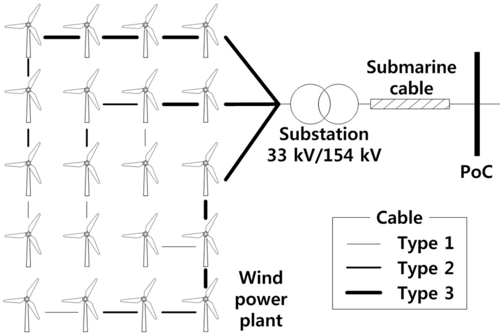
Figure 8.
System configuration for the case study. The system consists of 20 WTs with 5-MW capacity and includes harmonic filters.
The internal grid of the WPP adopts 33-kV line-to-line voltage and three types of submarine cables with different capacities as differentiated by the thickness of the lines connecting WTs in Figure 8. The equivalent π model is used for the submarine cable with parameters provided by the manufacturer. The frequency scan results of the two different cases are provided in Figure 9.
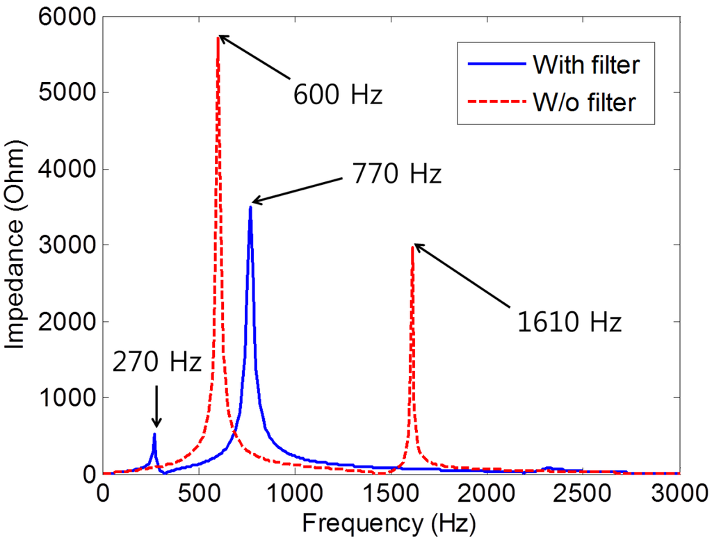
Figure 9.
Frequency scan result at the point of connection (PoC). This system has two dominant resonance points: at 270 Hz and 770 Hz. W/o: without.
Harmonic resonance occurs when a harmonic frequency coincides with a power system natural frequency. There are two forms of resonance, i.e., parallel and series resonances, and they can substantially distort voltage and amplify current [1,30]. As shown in Figure 9, without considering the PCS filter, the dominant resonance points are 600 Hz and 1610 Hz. However, they are moved to 270 Hz and 770 Hz, respectively, due to the effect of the PCS filters, which confirms that the PCS filters should be influential and carefully reflected in the harmonic resonance study. If the frequency of the external harmonic component coincides with the resonance frequency, the harmonic voltage can be magnified due to the parallel resonance. Harmonic data are collected at the PoC in Figure 8. Each harmonic magnitude is assumed to follow the normal distribution with its uniquely-identified parameters. In order to investigate the interactions of time-varying harmonics, resulting in harmonic cancellation or amplification, the changes of the standard deviation and interval size of the uniform distribution of the phase angle are taken into consideration. The details of the parameters are shown in the Appendix A. The random harmonic generation and FFT analysis are repeated every 0.2 s. The simulation study of this WPP scenario is carried out for 10 min (600 s), and 3000 samples of each harmonic component are analyzed.
5.2. Simulation Results of a Base Case
A base case model of the WPP is built based on the following scenarios: The standard deviation of each harmonic is 10% of its average value, and the phase angle is uniformly distributed with its interval size of . Very short time harmonic values (aggregation of 15 samples) and short time harmonic values (aggregation of 3000 samples) are obtained and assessed by the requirements in IEEE Std519-2014 [31]. Since there is no statement in the standard about inter-harmonics over 120 Hz, the recommended harmonic limit for the integer multiple of the fundamental frequency is applied to the inter-harmonic assessment. The 99th percentile very short time individual harmonic values from the base case are shown in Figure 10.
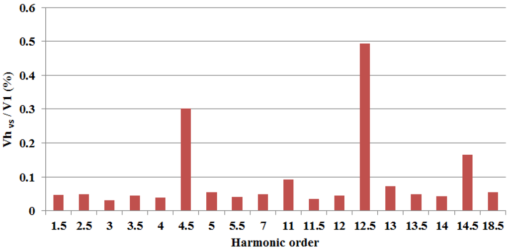
Figure 10.
Individual 99th percentile very short time harmonic values at the PoC of the WPP base case model.
Two largest harmonic components at the 4.5th and 12.5th order result from the two resonance points of the WPP with PCS filter. Figure 11 illustrates the histogram and the cumulative probability of the very short time voltage total harmonic distortion (THD) values. The THD varies in the range from 0.4676% to 0.6829%, and the 99th percentile THD value is 0.6482%, which satisfies the requirement of the IEEE standard.
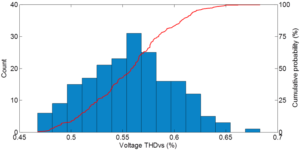
Figure 11.
Histogram and cumulative probability of very short time voltage total harmonic distortion (THD) values at the PoC of the WPP base case model.
5.3. Change of the Standard Deviation
A change in the standard deviation and its effect on the harmonics at the PoC are investigated. The ratio of the standard deviation of each harmonic PDF to its average value is changed from 0% to 20% with its phase angle interval size of . Figure 12 shows the maximum value (circle), minimum value (star), 99% very short time harmonic value (triangle) and short time harmonic value (square) of the largest individual harmonic distortion (IHD, 12.5th order) and the voltage THD at the PoC.
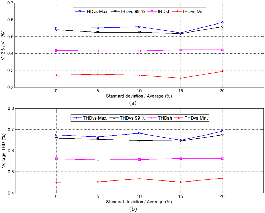
Figure 12.
The 12.5th order very short time individual harmonic distortion (IHD) and voltage THD in the variation of the standard variation: (a) 12.5th order; and (b) voltage THD.
The 99% IHD value is in the range from 0.5185% to 0.5582%, and IHD values in all cases are about 0.42%. The subtraction of the minimum from the maximum of THD ranges from 0.197% to 0.223%, and THD values are about 0.56%. All harmonic values in all of the cases comply with the requirements of the IEEE standard. Overall, IHD and THD in all cases vary in a similar range, even for the increased standard deviations, which results from the assumption that each harmonic generation is independent, and no correlation among harmonic components exits between the WTs. Stochastic and independent harmonic generation based on the normal distribution in 20 WTs causes the averaging effect on the harmonics at the PoC. Further studies incorporating the correlation among the WTs or harmonics in the same modeling framework may show different perspectives.
5.4. Change of the Interval Size of the Uniform Distribution of the Phase Angle
The phase angle of harmonics is still assumed to be uniformly distributed, and the interval size is now allowed to vary from zero to with 10% of the standard deviation over the average. For example, 90 degrees of the interval size means that the harmonic phase angle is generated in the range from zero to . Figure 13 shows the results of varying the interval size while other parameters are kept the same as in Figure 12.
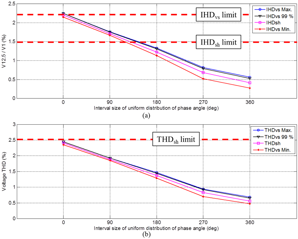
Figure 13.
The 12.5th order very short time IHD and voltage THD in the variation of the interval size of the phase angle: (a) 12.5th order; and (b) voltage THD.
The interval size variation is more influential on the harmonics at the PoC than the standard deviation change. IHD drops from 2.203% in the zero interval size to 0.4154% in the interval size, and THD decreases from 2.407% to 0.5589%. The difference between the maximum and minimum value steadily increases in both IHD and THD. Furthermore, with a zero interval size, which represents the worst case, the maximum IHD value is 2.246%, and THD is 2.407% close to the IEEE standard limit. Moreover, IHD values in the 0 and 90 interval sizes are over the IEEE limit. That is because there is no harmonic cancellation, and the harmonics are simply added at the PoC in the zero or 90 degree interval size. The wider the interval size, the higher the effect of harmonic cancellation. Therefore, the highest interval size shows the lowest harmonic magnitude.
6. Discussion
The proposed framework is designed to adopt the statistical information from the field measurements, if any. However, this framework can still be utilized in planning studies with, for example, simulation results with high-fidelity models. It is also worth noting the assumptions made in the study below: First, the correlation between the WT output power and harmonic magnitudes or between harmonic components is ignored because there is no consensus about the correlation related to the harmonics [7,8,9,15]. If any correlation between the harmonics is identified through measurements in operations, this needs to be incorporated in harmonic generation. Second, the uniform distribution is applied to the phase angle modeling. Although there is arguably no common rule for the phase angle modeling, the proposed framework can allow for different statistic models or a narrow interval size in a uniform distribution for phase angles. As shown in Figure 13, the narrow variation range of the phase angle results in the large harmonics at the PoC. Since the phase angle of the harmonic component is an important characteristic, illustrating natural harmonic cancellation at the PoC, the field measurements of the phase angles are desired and can improve the accuracy and validity of study result once they become available in operations. It is worth mentioning that the proposed framework can also synthesize the worst-case scenarios for investigation as needed by conditioning PDFs for magnitudes and phase angles of harmonic components, under which the harmonics from the WPP exceeded the limits in the case study.
7. Conclusions
This paper presented a study framework for capturing and evaluating stochastic harmonics and resonance concerns of wind integration. By exploiting the experimental data from the WT manufacturers or prior statistical information about harmonics from credible sources, we designed a harmonic current generator that represents the statistical characteristics of the harmonic currents from the WT and WPP. By incorporating the feeder configuration and the impact of harmonic filters, the variability of the wind and contingencies, etc., we can synthesize future operating scenarios and explore more credible cases, thus ensuring the grid compatibility of the WPP, especially when it is to be expanded. System operators can also comprehensively investigate the problematic operating conditions, in particular those that are unforeseen in the planning, and thus, systematically develop mitigation or correction measures.
Based on the framework above, we investigated harmonics and resonance issues of integrating a 100-MW offshore WPP consisting of 20 units of 5-MW full converter WTs benchmarking a WPP under development in Korea and concluded that the WPP would comply with the IEEE standards at the PoC. Based on the lessons learned from this study, the stochastic characteristics of the harmonics from the WTs could be exploited in taking any preventive measures against harmonics and resonance at this planning stage.
High penetrations of variable renewable sources into the electric power grid present a range of unprecedented grid operations and planning challenges requiring new study approaches and tools, so that the impacts of the proposed WPP can be properly assessed prior to interconnection. The proposed framework of interfacing statistical harmonics generation in the frequency domain and representation in the time domain simulation environment should be conceptually extended to other planning studies, especially those having harmonics and resonance issues. The research should help take advantage of prior knowledge to handle variability and offer opportunities for striking a balance between the technical and economic aspects of grid planning and operations.
Acknowledgments
This research was supported in part by the National Research Foundation of Korea (NRF) grant funded by the Korea government (MSIP) (No. 2010-0028509). This research was supported by Korea Electric Power Corporation through Korea Electrical Engineering & Science Research Institute. [grant number : R15XA03-28].
Author Contributions
Youngho Cho has developed the study framework and conducted simulation studies and written the paper with the support of Choongman Lee under supervision of the corresponding author, Kyeon Hur. Yong Cheol Kang and Eduard Muljadi helped improve the theoretical aspects and practicality of this study. Sang-Ho Park, Young-Do Choy and Gi-Gab Yoon supported the studies by providing transmission and manufacturers’ data and helped improve the study by adopting the study framework and providing comments.
Conflicts of Interest
The authors declare no conflict of interest.
Appendix A. Simulation Parameters
Parameters of test grid, harmonic filters and cable models used in the system studies are provided in Appendix A.

Table A1.
Grid parameters.
| Parameters | Values | Units |
|---|---|---|
| Grid frequency | 60 | Hz |
| X/R ratio | 4.5 | - |
| Short circuit capacity | 1525 | MVA |
Table A2.
Parameters of the harmonic filters.
| Parameters | Values | Units |
|---|---|---|
| Transformer capacity | 6.14 | MVA |
| Transformer leakage reactance | 10% | - |
| Filter reactor | 1.0 | mH |
| Filter capacitor | 200 | uF |
| Damping reactor | 0.12 | mH |
| Damping resistor | 0.6 | Ω |
| Converter switching frequency | 1 | kHz |
Table A3.
Parameters of the cable models.
| Types | Parameters | Values | Units |
|---|---|---|---|
| Type 1 | Resistance | 0.344 | Ω/km |
| Capacitance | 0.117 | uF/km | |
| Inductance | 0.456 | mH/km | |
| Type 2 | Resistance | 0.130 | Ω/km |
| Capacitance | 0.160 | uF/km | |
| Inductance | 0.393 | mH/km | |
| Type 3 | Resistance | 0.064 | Ω/km |
| Capacitance | 0.209 | uF/km | |
| Inductance | 0.350 | mH/km | |
| Submarine cable denoted in Figure 8 | Resistance | 0.056 | Ω/km |
| Capacitance | 0.141 | uF/km | |
| Inductance | 0.401 | mH/km |
References
- Bradt, M.; Badrzadeh, B.; Camm, E.; Mueller, D.; Schoene, J.; Siebert, T.; Smith, T.; Starke, M.; Walling, R. Harmonics and resonance issues in wind power plants. In Proceedings of the IEEE Power and Energy Society General Meeting, San Diego, CA, USA, 24–29 July 2011; pp. 1–8.
- Bollen, M.; Meyer, J.; Amaris, H.; Blanco, A.; Castro, A.; Desmet, J.; Klatt, M.; Kocewiak, L.; Rönnberg, S.; Yang, K. Future work on harmonics—Some expert opinions Part I—Wind and solar power. In Proceedings of the IEEE 16th International Conference on Harmonics and Quality of Power, Bucharest, Romania, 25–28 May 2014; pp. 904–908.
- Negnevitsky, M.; Nguyen, D.; Piekutowski, M. Risk assessment for power system operation planning with high wind power penetration. IEEE Trans. Power Syst. 2015, 30, 1359–1368. [Google Scholar] [CrossRef]
- Zhang, S.; Tseng, K.; Choi, S. Statistical voltage quality assessment method for grids with wind power generation. IET Renew. Power Gener. 2010, 4, 43–54. [Google Scholar] [CrossRef]
- Xie, G.; Zhang, B.; Li, Y.; Mao, C. Harmonic propagation and interaction evaluation between small-scale wind farms and nonlinear loads. Energies 2013, 6, 3297–3322. [Google Scholar] [CrossRef]
- Yang, K.; Bollen, M.; Larsson, E.; Wahlberg, M. Measurement of harmonic emission versus active power from wind turbines. Electr. Power Syst. Res. 2014, 108, 304–314. [Google Scholar] [CrossRef]
- Sainz, L.; Mesas, J.; Teodorescu, R.; Rodriguez, P. Deterministic and stochastic study of wind farm harmonic currents. IEEE Trans. Energy Conver. 2010, 25, 1071–1080. [Google Scholar] [CrossRef]
- Tentzerakis, S.; Papathanassiou, S. An investigation of the harmonic emissions of wind turbines. IEEE Trans. Energy Conver. 2007, 22, 150–158. [Google Scholar] [CrossRef]
- Kocewiak, L. Harmonics in Large Offshore Wind Farms. Ph.D. Thesis, Deptartment of Energy Techonology, Aalborg University, Aalborg, Denmark, 2012. [Google Scholar]
- Baghzouz, Y.; Burch, R.; Capasso, A.; Cavallini, A.; Emanuel, A.; Halpin, M.; Imece, A.; Ludbrook, A.; Montanari, G.; Olejniczak, K.; et al. Time-varying harmonics. I. Characterizing measured data. IEEE Trans. Power Deliv. 1998, 13, 938–944. [Google Scholar] [CrossRef]
- Mau Teng, A.; Milanovic, J. Development of stochastic aggregate harmonic load model based on field measurements. IEEE Trans. Power Deliv. 2007, 22, 323–330. [Google Scholar]
- Foiadelli, F.; Pinato, P.; Zaninelli, D. Statistical model for harmonic propagation studies in electric traction supply systems. In Proceedings of the 11th International Conference on Harmonics and Quality of Power, Lake Placid, NY, USA, 12–15 September 2004; pp. 753–758.
- Kocewiak, L.; Bak, C.; Hjerrild, J. Statistical Analysis and Comparison of Harmonics Measured in Offshore Wind Farms. In Proceedings of the European Wind Energy Association OFFSHORE 2011, Amsterdam, The Netherlands, 29 November–1 December 2011; pp. 1–10.
- Cavallini, A.; Montanari, G. A deterministic/stochastic framework for power system harmonics modeling. IEEE Trans. Power Syst. 1997, 12, 407–415. [Google Scholar] [CrossRef]
- Teng, J.; Leou, R.; Chang, C.; Chan, S. Harmonic current predictors for wind turbines. Energies 2013, 6, 1314–1328. [Google Scholar] [CrossRef]
- Badrzadeh, B.; Gupta, M. Practical experiences and mitigation methods of harmonics in wind power plants. IEEE Trans. Ind. Appl. 2013, 49, 2279–2289. [Google Scholar] [CrossRef]
- Patel, D.; Varma, R.; Seethapathy, R.; Dang, M. Impact of wind turbine generators on network resonance and harmonic distortion. In Proceedings of the Canadian Conference on Electrical and Computer Engineering, Calgary, AB, Canada, 2–5 May 2010; pp. 1–6.
- Hasan, K.; Rauma, K.; Rodriguez, P.; Candela, J.; Munoz-Aguilar, R.; Luna, A. An overview of harmonic analysis and resonances of large wind power plant. In Proceedings of the IECON 2011—37th Annual Conference on IEEE Industrial Electronics Society, Melbourne, VIC, Australia, 7–10 November 2011; pp. 2467–2474.
- Yang, K.; Bollen, M.; Anders Larsson, E. Aggregation and amplification of wind-turbine harmonic emission in a wind park. IEEE Trans. Power Deliv. 2015, 30, 791–799. [Google Scholar] [CrossRef]
- Huan, C.X.; Tayjasanant, T. Modeling wind power plants in harmonic resonance study—A case study in Thailand. In Proceedings of the International Conference on Information Technology and Electrical Engineering, Yogyakarta, Indonesia, 7–8 October 2013; pp. 385–390.
- Baghzouz, Y.; Burch, R.; Capasso, A.; Cavallini, A.; Emanuel, A.; Halpin, M.; Langella, R.; Montanari, G.; Olejniczak, K.; Ribeiro, P.; et al. Time-varying harmonics: Part II. Harmonic summation and propagation. IEEE Trans. Power Deliv. 2002, 17, 279–285. [Google Scholar] [CrossRef]
- Wind Turbine Generator Systems-Part 21: Measurement and Assessment of Power Quality Characteristics of Grid Connected Wind Turbines; IEC 61400-21; International Electrotechnical Commission: Geneva, Switzerland, 2001.
- Papathanassiou, S.; Papadopoulos, M. Harmonic analysis in a power system with wind generation. IEEE Trans. Power Deliv. 2006, 21, 2006–2016. [Google Scholar] [CrossRef]
- Medeiros, F.; Brasil, D.; Ribeiro, P.F.; Marques, C.; Duque, C. A new approach for harmonic summation using the methodology of IEC 61400-21. In Proceedings of the 14th International Conference on Harmonics and Quality of Power, Bergamo, Italy, 26–29 September 2010; pp. 1–7.
- Yates, R.; Goodman, D. Probability and Stochastic Process, 2nd ed.; Wiley: Hoboken, NJ, USA, 2005. [Google Scholar]
- Myung, I. Tutorial on maximum likelihood estimation. J. Math. Psychol. 2003, 47, 90–100. [Google Scholar] [CrossRef]
- Keller, G. Managerial Statistics, 9th ed.; South-Western Cengage Learning: Mason, OH, USA, 2011. [Google Scholar]
- Electromagnetic Compatibility (EMC)-Part 4-7: Testing and Measurement Techniques-General Guide on Harmonics and Interharmonics Measurements and Instrumentation, for Power Supply Systems and Equipment Connected Thereto; IEC 61000-4-7; International Electrotechnical Commission: Geneva, Switzerland, 2002.
- Mendonça, G.; Pereira, H.; Silva, S. Wind farm and system modelling evaluation in harmonic propagation studies. In Proceedings of the International Conference on Renewable Energies and Power Quality, Santiago de Compostela, Spain, 28–30 March 2012; pp. 1–6.
- Dugan, R.; Mcgranaghan, M.; Santoso, S.; Beaty, H. Electrical Power Systems Quality, 3rd ed.; McGraw-Hill: New York, NY, USA, 2012. [Google Scholar]
- IEEE Recommended Practice and Requirements for Harmonic Control in Electric Power Systems; IEEE Std 519; IEEE Standards Association: New York, NY, USA, 2014.
© 2016 by the authors; licensee MDPI, Basel, Switzerland. This article is an open access article distributed under the terms and conditions of the Creative Commons Attribution (CC-BY) license (http://creativecommons.org/licenses/by/4.0/).