Optimal Energy Management, Location and Size for Stationary Energy Storage System in a Metro Line Based on Genetic Algorithm

Abstract

The installation of stationary super-capacitor energy storage system (ESS) in metro systems can recycle the vehicle braking energy and improve the pantograph voltage profile. This paper aims to optimize the energy management, location, and size of stationary super-capacitor ESSes simultaneously and obtain the best economic efficiency and voltage profile of metro systems. Firstly, the simulation platform of an urban rail power supply system, which includes trains and super-capacitor energy storage systems, is established. Then, two evaluation functions from the perspectives of economic efficiency and voltage drop compensation are put forward. Ultimately, a novel optimization method that combines genetic algorithms and a simulation platform of urban rail power supply system is proposed, which can obtain the best energy management strategy, location, and size for ESSes simultaneously. With actual parameters of a Chinese metro line applied in the simulation comparison, certain optimal scheme of ESSes’ energy management strategy, location, and size obtained by a novel optimization method can achieve much better performance of metro systems from the perspectives of two evaluation functions. The simulation result shows that with the increase of weight coefficient, the optimal energy management strategy, locations and size of ESSes appear certain regularities, and the best compromise between economic efficiency and voltage drop compensation can be obtained by a novel optimization method, which can provide a valuable reference to subway company.

1. Introduction

In recent years, with the rapid development of the Chinese economy, growing environmental pollution, and traffic congestion in major cities are becoming serious social issues. For the purpose of improving the urban environment and energy efficiency, the development of modern urban rail transit, which has the significant advantages of large capacity, punctuality, safety, energy conservation, and environmental protection, becomes a social consensus [1,2]. Low running resistance and the reuse of braking energy are two main factors that make urban rail transit better than other means of transport in energy efficiency. Recent studies have shown that up to 40% of the energy supplied to electrical rail guided vehicles could be recovered through regenerative braking [1]. In a metro network system, the trains are accelerated and braked frequently. Since most of the rectifiers in the metro network are unidirectional, the regenerative braking energy cannot be returned to the supply network, and if there are no adjacent accelerating trains or energy storage system to absorb the regenerative energy, the surplus braking energy has to be wasted on the mechanical braking or on-board resistors. If different trains are close to each other and they start all together, contact lines will become overloaded and the pantograph voltages of trains will drop significantly, which results in high lines loss and the opening of minimum voltage protective action of trains by limiting the current. Hence, the installation of energy storage systems in urban railway transit has become a universal concern, which can recycle the regenerative braking energy, prevent regeneration cancellation, shave the peak power of substations, and compensate the voltage drops of pantograph quickly.

Current research activities have presented the application of batteries, flywheels, super-capacitors, and hybrid energy storages as energy storage devices [3,4,5,6,7,8]. Among the different storage systems available, super-capacitors seem to be the most appropriate for the application in a metro system for the advantages of rapid charging and discharging frequencies, a long cycle life, and high power density, which highly match the characteristics of metro system, such as short running time between stations, frequent accelerating and braking, booming power within a short time, etc. Super-capacitor energy storage systems (ESS) can be either stationary or on-board [8,9,10,11]. The allocation on board of the storage system increases the train mass and requires additional space for their accommodation. Thus, stationary ESSes set inside traction substations (TSSs) are preferred for metro systems, and their best energy management, location, and size will be discussed in this paper.

Several papers have dealt in depth with optimization of energy management strategies of stationary ESSes [12,13,14]. Among them [12] proposes a control strategy based on the maximum kinetic energy recovery throughout braking operations of the running vehicles. The strategy stays on the knowledge of the state of charge of ESS and the actual vehicle speeds. Reference [13] proposes a optimization procedure based on a linearized modeling of the electrical LRV network, the target of the control strategy is the optimal tracking of the storage device voltage subject to the minimization of the substations supplied power. Optimal location and size of ESSes are also investigated in detail in [15,16,17,18,19,20,21,22]. Reference [15] discusses the configuration of ESSes for voltage drop compensation, which takes account of the topology of the line and the movement of the vehicles. Reference [16] proposes an optimization method based on a genetic algorithm, which can obtain certain preferable location and size for ESSes.

However, there are still some drawbacks on the above research. Firstly, some of the references involve only small amounts of substations and vehicles when modeling the urban railway network [12,13,14,15] and some of them do not take into account the time-variation (network topology change with vehicle movement) and nonlinearity (nonlinearity of substation and regenerative braking) of the network structure. Secondly, and most importantly, the optimization research of energy management strategy and configuration for ESSes will influence each other, and they both affect the performances of urban railway network, while the configuration optimization research of ESSes in reference [16,17,18,19,20,21,22] is on the premise that energy management strategy of ESSes is fixed and invariable.

In this paper improved energy management strategy of ESSes and novel optimization method are proposed. Compared to previous work [16,17,18,19,20,21,22], the improved energy management strategy can manage and coordinate the energy flow of multiple ESSes, which can achieve smoother changes of voltages and currents in the system and improve the energy savings of ESSes effectively, and the new proposed optimization algorithm can further improve the performance of ESSes by optimizing energy management parameters, location, and size of ESSes simultaneously, which has rarely been studied in previous work about the optimization of ESSes, and the evaluation functions of proposed optimization algorithm in this paper are more appropriate, which are put forward from the perspectives of economic efficiency and voltage drop compensation.

The organization of this work is as follow: the simulation platform of urban rail power supply system, which includes trains and super-capacitor energy storage systems has been established in Section 2; additionally, particular data of the researched Chinese metro line is given. Then Section 3 sets up two evaluation functions from the perspectives of economic efficiency and voltage drop compensation. In Section 4, a novel optimization method based on genetic algorithm (GA) is put forward, which can optimize energy management strategy, location and size of ESSes simultaneously. Finally in Section 5, the result of the simulation comparison is presented and discussed.

2. Modeling

2.1. Model of Metro Power Supply Network

The model of metro system’s DC traction power supply network is shown in Figure 1 [16]. In order to show the behavior of the metro power supply network as correctly as possible, all components of the metro network, which includes irreversible traction substations (TSS), trains, metro lines, and stationary energy storage systems (ESSes), will be modeled appropriately to maintain original characters of the network structure’s time-variation and nonlinearity.

Figure 1. The model of metro system’s DC traction power supply network.

Figure 1. The model of metro system’s DC traction power supply network.

2.1.1. Traction Substation (TSS) Model

As shown in Figure 2, the substation is modeled by an ideal DC voltage source connected in series with its equivalent internal resistance R_S and the diode D, which to simulate output characteristics. When the output current of substation is increased, the voltage of substation decreases correspondingly to limit its output power. U₀ is the no-load voltage of substations.

$$i_{\text{uout}}=i_{\text{uin}}+i_{\text{din}}+i$$

(1)

$$i=i_{\text{uc}}+i_{\text{sub}}$$

(2)

$$i_{\text{sub}}\ge 0$$

(3)

Figure 2. TSS model.

Figure 2. TSS model.

2.1.2. Train Model

As shown in Figure 3, the train model is modeled by a controlled current source which draws electric power at the accelerating time and delivers braking power at the regenerative time. The impedance of the line connected to the trains is expressed as Z, the value of which is time-varying, and it is linear with the line length that is determined by the present position of trains. When pantograph voltage exceeds U_b, the braking resistor R_b will consume the braking energy. R_f is vehicle filter resistance; L_f is vehicle filter inductance; C_fc is the support capacitor of train; P_aux is auxiliary power; and P is the electric power of train.

$$u_{\text{out}}=u_{\text{in}}+R{i}_{\text{out}}+L\frac{d{i}_{\text{out}}}{dt}$$

(4)

$$i_{\text{out}}=i_{\text{in}}+i$$

(5)

$$i=-i_{inv}-\frac{p_{aux}}{u_{fc}}-C_{fc}\frac{d{u}_{fc}}{dt}$$

(6)

Figure 3. Train model.

Figure 3. Train model.

2.1.3. Energy Storage System (ESS) Model

The ESS model consists of the super-capacitors, controlled current source, and energy management strategy controller, is shown in Figure 4. The ESS model is connected in parallel with the output of the substation, and it can deliver or draw the electric power from the metro power supply network through the current source which is controlled by the energy management strategy and configuration of super-capacitors in real time.

Figure 4. Stationary ESS model.

Figure 4. Stationary ESS model.

The SOC (State of Charge) of super-capacitors is defined as follows, it represents the storage energy of ESS, which is proportional to the square of the terminal voltage.

$$0.25\le SOC=\frac{E_{\text{sc}}}{E_{\text{scmax}}}=\frac{0.5C{U}_{\text{sc}}^{\text{2}}}{0.5C{U}_{s\text{cmax}}^2}=\frac{U_{\text{sc}}^{\text{2}}}{U_{s\text{cmax}}^2}\le 1$$

(7)

In a practical application, the function of controlled current source in the model is generally implemented by the unidirectional DC/DC converter. In order to maintain the normal operation of DC/DC converter, the terminal voltage of super-capacitors should be set between 50% and 100% the maximum voltage, so the range of SOC varies from 0.25 to 1.

2.2. Simulation Platform of Metro System for Power Flow Calculation

As above, the model of a DC metro power supply network (DC-PSN) is set up by a novel approach of component segmentation. In order to calculate the power flow of the DC metro power supply network, an integrated simulation platform, which includes DC metro power supply network (DC-PSN), train performance simulator (TPS), and super-capacitor energy storage system (SCESS) is established in the Matlab environment, as shown in Figure 5 [16].

Figure 5. Simulation platform of metro system for power flow calculation.

Figure 5. Simulation platform of metro system for power flow calculation.

2.2.1. DC Metro Power Supply Network (DC-PSN)

In the previous section, the paper has presented the structure and model of a DC-PSN. In the power flow calculation of the DC metro power supply network, because of its time-variation (network topology changes with train movement) and nonlinearity (nonlinearity of substation and regenerative braking) of the network structure, a new power flow calculation method by component segmentation is presented. The simulation result shows excellent rapidity and astringency can be obtained by this method. Moreover, the structure and model of the DC-PSN can be extended easily.

2.2.2. Train Performance Simulator (TPS)

As shown in Figure 5, the output of TPS is not only associated with line condition, vehicle data, and timetable, but is also constrained by real-time train pantograph voltage. From the TPS we can get positions of up-line and down-line trains and their corresponding electric power, which offer essential data for subsequent power flow calculation of the DC supply network.

2.2.3. Super-Capacitor Energy Storage System (SCESS)

SCESS set certain energy management strategy, location, and size of ESSes on different substations, which determine the power direction and value of ESSes in real time. The installation of ESSes will change the power flow of the DC metro power supply network and the system performances can be improved significantly by setting the most appropriate energy management strategy, location, and size.

2.3. Case Data

A particular case of Beijing Subway line is studied in this paper. The total length of the line is about 11.3 km along with 12 stations, of which seven are traction substations and their distribution is shown in Table 1. The vehicle data and metro DC network parameters are shown as Table 2. These parameters are provided by the Beijing Subway Company.

Table 1. TSS spacing distances.

Traction substation	1–2	2–3	3–4	4–5	5–6	6–7
Substation spacing (km)	1.1	1.9	2.2	2.3	2.1	2.7

Table 1. TSS spacing distances.

Traction substation	1–2	2–3	3–4	4–5	5–6	6–7
Substation spacing (km)	1.1	1.9	2.2	2.3	2.1	2.7

Table 2. Vehicle data.

Parameter	Value	Parameter	Value
Formation	3M3T	Inverter efficiency	0.97
Load condition	312.9t (AW3)	Motor efficiency	0.915
Rated voltage	750 Volt	Gearing efficiency	0.93
AC motor/M	180 kW × 4	Max speed	80 km/h
SIV power	160 kVA × 2	Max acceleration	1 m/s2
SIV power factor	0.85	Min deceleration	−1 m/s2
Floating voltage Us	836 Volt	Equivalent internal resistance Rs	0.07 Ω
Contract line impendence	0.007 Ω/km	Rail impendence	0.009 Ω/km
Pantograph impendence	0.015 Ω	–	–

Table 2. Vehicle data.

Parameter	Value	Parameter	Value
Formation	3M3T	Inverter efficiency	0.97
Load condition	312.9t (AW3)	Motor efficiency	0.915
Rated voltage	750 Volt	Gearing efficiency	0.93
AC motor/M	180 kW × 4	Max speed	80 km/h
SIV power	160 kVA × 2	Max acceleration	1 m/s2
SIV power factor	0.85	Min deceleration	−1 m/s2
Floating voltage Us	836 Volt	Equivalent internal resistance Rs	0.07 Ω
Contract line impendence	0.007 Ω/km	Rail impendence	0.009 Ω/km
Pantograph impendence	0.015 Ω	–	–

2.4. Simulation Output

Under simulation conditions, super-capacitor ESSes of 14 kWh are configured in every other substation and controlled with a traditional double-loops control strategy [16]. The simulation output waveforms is shown in Figure 6, which include speed and electric power of an up-line train, voltage and current of the train pantograph, voltage and current of a substation, charging energy, and SOC of the ESS in the substation. SOC of ESS varies between 0.25 and 1.

Figure 6. The output waveforms of simulation platform.

Figure 6. The output waveforms of simulation platform.

3. Objective Function

3.1. Objective Function

In order to evaluate the system performances in terms of energy saving, voltage drop compensation, and installation cost for different energy management strategy and configuration of ESSes, the paper puts forward two evaluation functions and one objective function.

3.1.1. Economic Efficiency, $e\%$

Economic efficiency $e\%$ is put forward from the viewpoint of considering energy savings and installation cost in a unified way to evaluate the economic return rates of ESSes for Subway Company. Economic efficiency $e\%$ is a percentage calculated by dividing the total electricity price of the substations by economic savings (returns minus costs).

As shown in Figure 7, one super-capacitor ESS, which includes the connection unit, DC/DC converter, and super-capacitor strings, is installed on the traction substation. The circuit structure of super-capacitor ESS is shown in Figure 8. The installation cost of ESSes is determined by various factors, which include the capacity, equipment, control circuit, maintenance cost, etc. The cost of DC/DC converters and super-capacitor strings are determined mainly by the maximum power of the ESS. In order to ease the DC/DC converter design, maximum voltage of super-capacitor strings should be lower than network voltage (836 V at no load). Hence, six super-capacitor modules (BMOD0063P125) are put in series to form a super-capacitor string, which has terminal voltage of 750 V and maximum continuous power of 180 kW, and the configuration of super-capacitors installed in every substation could be adjusted by changing the number of paralleled super-capacitor strings. The Parameters of super-capacitor modules (BMOD0063P125) are shown as Table 3.

Figure 7. Super-capacitor ESS installed in traction substation.

Figure 7. Super-capacitor ESS installed in traction substation.

Figure 8. The circuit structure of super-capacitor ESS.

Figure 8. The circuit structure of super-capacitor ESS.

Table 3. Parameters of super-capacitor module (BMOD0063P125).

Parameter	Value	Parameter	Value
Rated voltage	125 V	Capacitance	63 F
Maximum continuous current	240 A	Maximum continuous power	30 kW
Maximum ESRDC, initial	0.018 Ω	Energy	0.137 kWh
Price	5,333 $

Table 3. Parameters of super-capacitor module (BMOD0063P125).

Parameter	Value	Parameter	Value
Rated voltage	125 V	Capacitance	63 F
Maximum continuous current	240 A	Maximum continuous power	30 kW
Maximum ESRDC, initial	0.018 Ω	Energy	0.137 kWh
Price	5,333 $

The cost of investment for a super-capacitor ESS on substation k during their life time of l years, can be calculated by:

$$Cos{t}_k=\{\begin{array}{l}0,n_k=0\\ \left(C+n_k\times p\times m\right)\times {\left(1+r\right)}^l,0<n_k\le 18\end{array}$$

(8)

where n_k is the number of paralleled super-capacitor strings on substation k; p is the maximum power of one super-capacitor string; and m is dollar per power constant for super-capacitors and DC/DC converter. If n_k equals 0, a super-capacitor ESS would not be installed on substation k. If n_k is more than 0, the cost of investment for super-capacitor ESS Cost_k includes two parts. $n_k\times p\times m$ is the cost of DC/DC converters and super-capacitor strings that are determined by the maximum power of the ESS; C is other part of installation cost from protective device, breaker, maintenance cost, etc., which has a small relationship to power of the ESS. r is the rate of return constant. Considering the limited free space of each metro substation, the number of paralleled super-capacitor strings n_k on each substation is no bigger than 18 in this paper.

By taking the sum of output energy consumption of all TSSes along the metro line, the total energy consumption of the substations in kWh during one year can be calculated from the following formula:

$$E_{\text{sub}}={\displaystyle \sum _1^k\left[{\displaystyle {\int }_0^T(I_{\text{sub}}\cdot U_{\text{sub}})dt}\right]}\times \frac{365}{3600000}$$

(9)

where k is the number of traction substations; T is the running time in one day. U_sub, I_sub are, respectively, the voltage and current of substation.

The application of ESSes in a metro system can reduce the total energy consumption of the substations because of the recycle of trains’ regenerative braking energy, but the installation cost should also be considered as well. The total profit obtained by ESSes in l years should be the difference between the saved electricity price and the installation cost of ESSes.

$$P_{\text{sub}}^{\text{nosc}}=E_{\text{sub}}^{\text{nosc}}\times \epsilon \times \frac{l\left(2+\left(l-2\right)i\right)}{2}$$

(10)

where $E_{\text{sub}}^{\text{nosc}}$ is one year energy consumption of the substations in absence of ESSes; $\epsilon$ is electricity price in dollar per kWh, $P_{\text{sub}}^{\text{nosc}}$ is l years’ electricity price of the substations in absence of ESSes, and i is the yearly inflation of electricity price.

$$P_{\text{sub}}^{\text{sc}}=E_{\text{sub}}^{\text{sc}}\times \epsilon \times \frac{l\left(2+\left(l-2\right)i\right)}{2}+{\displaystyle \sum _1^{k}Cos{t}_k}$$

(11)

where $E_{\text{sub}}^{\text{sc}}$ is one year’ energy consumption of the substations in presence of ESSes, $Cos{t}_k$ is installation cost of ESS on substation k, and $P_{\text{sub}}^{\text{sc}}$ is l years’ expenditure of the substations in presence of ESSes, which includes the electricity price and installation cost of ESSes.

In this paper, economic efficiency $e\%$ is defined as the following formula:

$$e\%=\frac{P_{\text{sub}}^{\text{nosc}}-P_{\text{sub}}^{\text{sc}}}{P_{\text{sub}}^{\text{nosc}}}\times 100\%$$

(12)

when economic efficiency $e\%$ equals 0, it means the saved electricity price is the same as the installation cost of ESSes. Necessary parameters for calculating the economic efficiency $e\%$ of ESSes are given in Table 4.

Table 4. Necessary parameters for calculating economic efficiency.

Parameter	Value	Parameter	Value
p	180 kW	$\epsilon$	0.16 $/kWh
m	0.244 $/W	r	5%
C	0.16 M$	i	5%
l	10 years

Table 4. Necessary parameters for calculating economic efficiency.

Parameter	Value	Parameter	Value
p	180 kW	$\epsilon$	0.16 $/kWh
m	0.244 $/W	r	5%
C	0.16 M$	i	5%
l	10 years

3.1.2. Voltage Drop Compensation, $v\%$

If different trains are close to each other and they start all together, contact lines will become overloaded and the pantograph voltages of trains will drop significantly, which results in high line loss and the opening of minimum voltage protective action of trains by limiting the current. The installation of ESSes in the metro system can shave the peak power of substations, improve the load capacity of the system, and compensate the pantograph drops quickly. Voltage drop compensation $v\%$, in this paper, evaluates in percent the voltage drop compensation at the pantograph, giving the rate about how much the voltage drops improvement is when the ESSes are installed.

$$v\%=\frac{{\displaystyle {\sum }_1^j{\displaystyle {\int }_{U_p<U_r}\left(U_r-U_p^{nosc}\right)}dt}-{\displaystyle {\sum }_1^j{\displaystyle {\int }_{U_p<U_r}\left(U_r-U_p^{sc}\right)}dt}}{{\displaystyle {\sum }_1^j{\displaystyle {\int }_{U_p<U_r}\left(U_r-U_p^{nosc}\right)}dt}}\times 100\%$$

(13)

where, Up is the pantograph voltage of trains; Ur is the rated voltage of trains’ pantograph; j is the amount of up-line and down-line trains. From the Equation (14), voltage drop compensation $v\%$ is calculated based on the integral of voltage drops improvement when Up is less than Ur, which is more appropriate and comprehensive than the maximum voltage drop compensation just in a moment in [15].

3.1.3. Objective Function, ObjV

Given economic efficiency $e\%$ and voltage drop compensation $v\%$, the objective function for optimal energy management strategy and configuration of ESSes is shown as below:

$$ObjV=\text{ω}\times e\%+(1-\text{ω})\times v\%$$

(14)

where $\text{ω}$ is the weight coefficient of economic efficiency $e\%$, it represents the emphasis degrees of economic efficiency $e\%$. When $\text{ω}$ is set to 1, it means that economic efficiency is the only evaluation index considered in the optimization.

4. Novel Optimization Method Based on a Genetic Algorithm

The traditional optimization method based on a genetic algorithm proposed in [16] can optimize the location and size of ESSes significantly, but the adopted energy management strategy is constant. The energy management is also important for the performance improvement of a metro supply network, and the optimization of energy management and configuration for ESSes will influence each other. Thus, the proposed novel optimization method in this paper, which combines a genetic algorithm and a simulation platform of urban rail power supply system, is meant to optimize energy management, location, and size of ESSes simultaneously.

4.1. Improved Energy Management Strategy

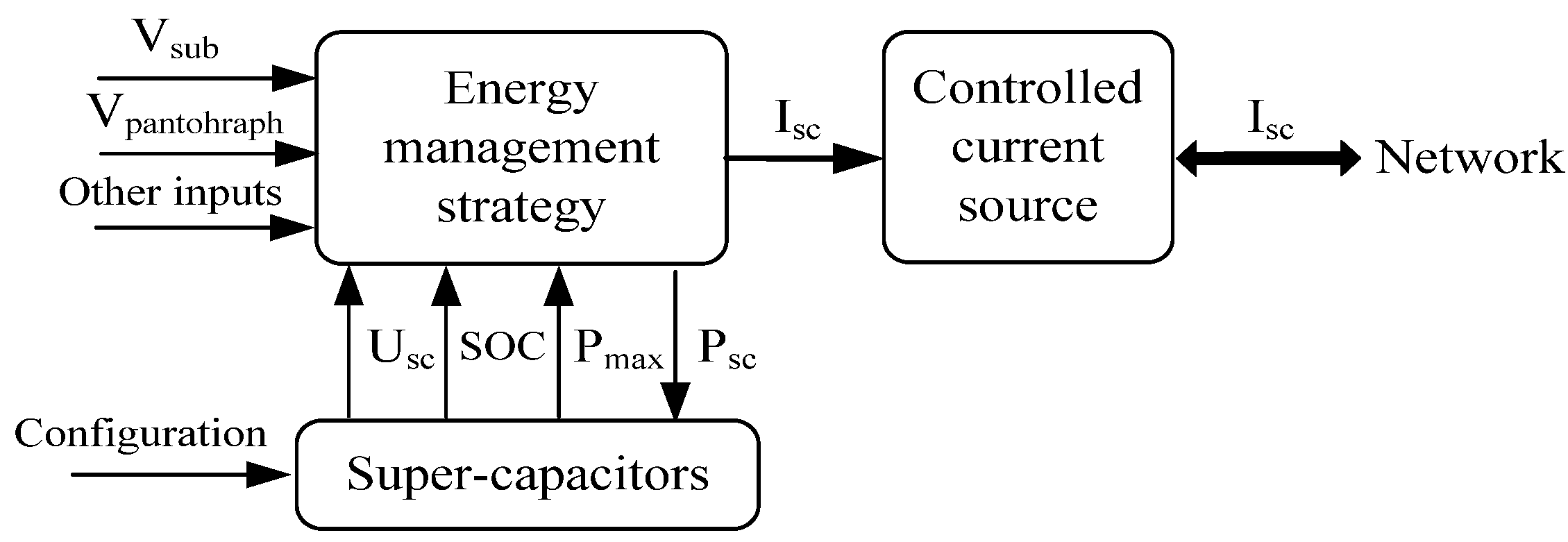
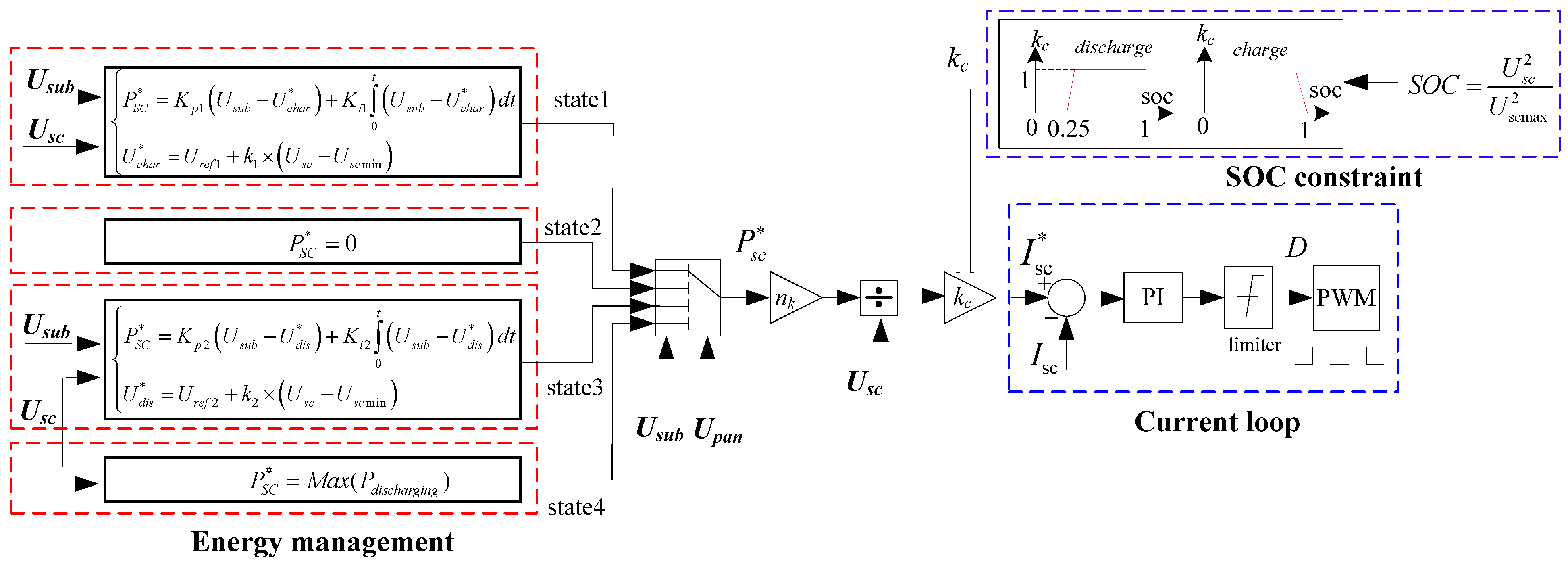
In order to improve economic efficiency $e\%$ and voltage drop compensation $v\%$ of ESSes, an improved energy management strategy is put forward, which decides the charging and discharging current of the ESS by detecting the voltage of substation, ESS and train pantographs, as shown in Figure 9.

The improved energy management strategy can be divided into three parts: SOC constraint, current loop, and energy management. Due to the function of the SOC constraint, the working range of the SOC is 0.25–1, and the terminal voltage of ESSes is limited between 375 V and 750 V. Energy management can switch four work states to produce appropriate reference P_sc* for the ESS according to the substation voltage and pantograph voltage of the trains. The current loop can control the charging and discharging current of the super-capacitor ESS according to the reference I_sc*.

Figure 9. The improved energy management strategy of stationary ESSes.

Figure 9. The improved energy management strategy of stationary ESSes.

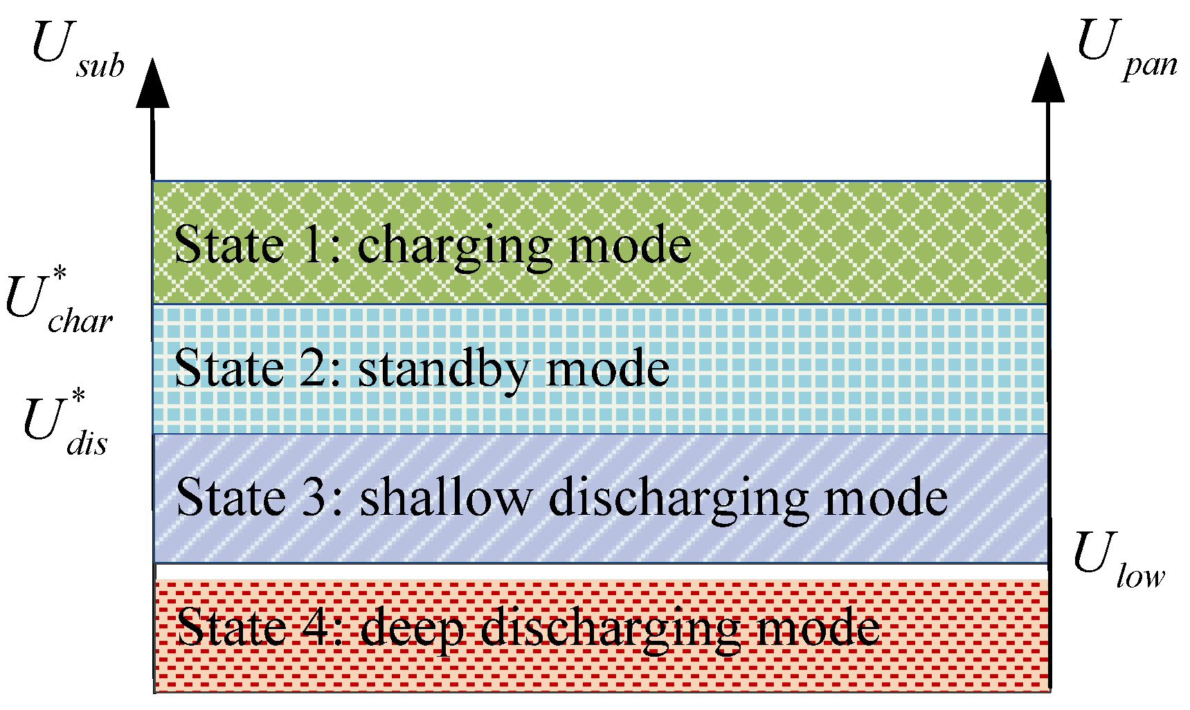
The charging and discharging current reference I_sc* of the super-capacitor ESS can be calculated by Equation (15). And work states of super-capacitor ESS are shown in Figure 10.

$$I_{sc}^{*}=\frac{n_k\times k_c\times P_{sc}^{*}}{U_{sc}}$$

(15)

Figure 10. Work states of super-capacitor ESS.

Figure 10. Work states of super-capacitor ESS.

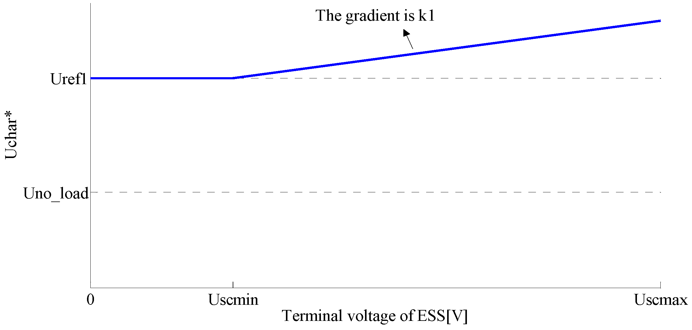
State 1: When the voltage of substation is higher than charging threshold value U_char*, the magnitude of the charging current reference P_sc* is determined by the PI controller according to the difference value between the present substation voltage and the threshold value U_char*. From Equation (16), if the electric braking power of train is small, the super-capacitor ESS will absorb all the regenerative braking energy and maintain the substation voltage at U_char*. Then, if the electric braking power of train is excessive, the super-capacitor ESS will absorb the braking energy with maximum charging current. The value of U_char* will increase with the increase of ESSes’ terminal voltage, which enlarges the charging current of ESSes with smaller terminal voltage of ESSes significantly, as shown in Figure 11. The value of U_scmin is set to 375 V in this paper.

$$\{\begin{array}{l}{P}_{sc}^{*}=K_{p1}\times \left(U_{sub}-U_{char}^{*}\right)+K_{i1}\times {\displaystyle \underset{0}{\overset{t}{\int }}\left(U_{sub}-U_{char}^{*}\right)dt}\\ U_{char}^{*}=U_{ref1}+k_1\times \left(U_{sc}-U_{sc\min }\right)\\ K_{p1}\ge 0,K_{i1}\ge 0,U_{char}^{*}>U_{no\_load},k_1\ge 0,U_{sc\max }\ge U_{sc}\ge U_{sc\min }\end{array}$$

(16)

Figure 11. The values of U_char^*.

Figure 11. The values of U_char^*.

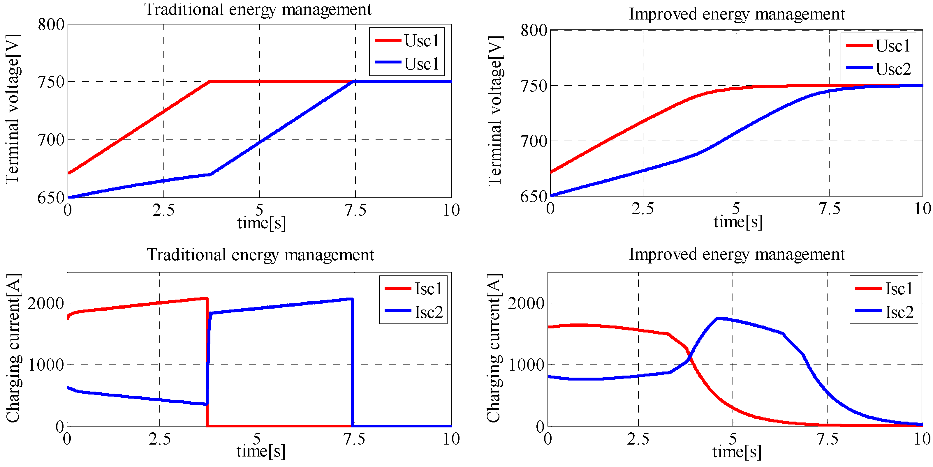
When the train is braking in one substation, by traditional energy management, the ESS installed in the substation will draw high power of regenerative energy and take no account of its terminal voltage and stored energy [16]. When the ESS is charged up to 100% with the regenerative energy, its terminal voltage would be 750 V and its charging current will be interrupted instantaneously, which leads to the drastic changes of substation current and line current, then all the regenerative energy of trains flows to the ESSes in the near substations as shown in Figure 12. ESSes are charged in turn and both with large current. On the contrary, by the improved energy management strategy, the ESS can adjust the threshold value U_char* according to its terminal voltage and achieve smoother changes of terminal voltage and charging current. Consequently, the regenerative energy is distributed to ESSes more evenly. It is worth mentioning that the improved energy management strategy reduces the line loss greatly and it also contributes to balance the terminal voltage for all different strings of ESS on a substation.

Figure 12. Terminal voltage and charging current of ESSes.

Figure 12. Terminal voltage and charging current of ESSes.

State 2: When the voltage of substation fluctuates between the charging threshold value U_char* and the discharging threshold value U_dis*, super-capacitor ESS maintain the standby state.

$$P_{SC}^{*}=0$$

(17)

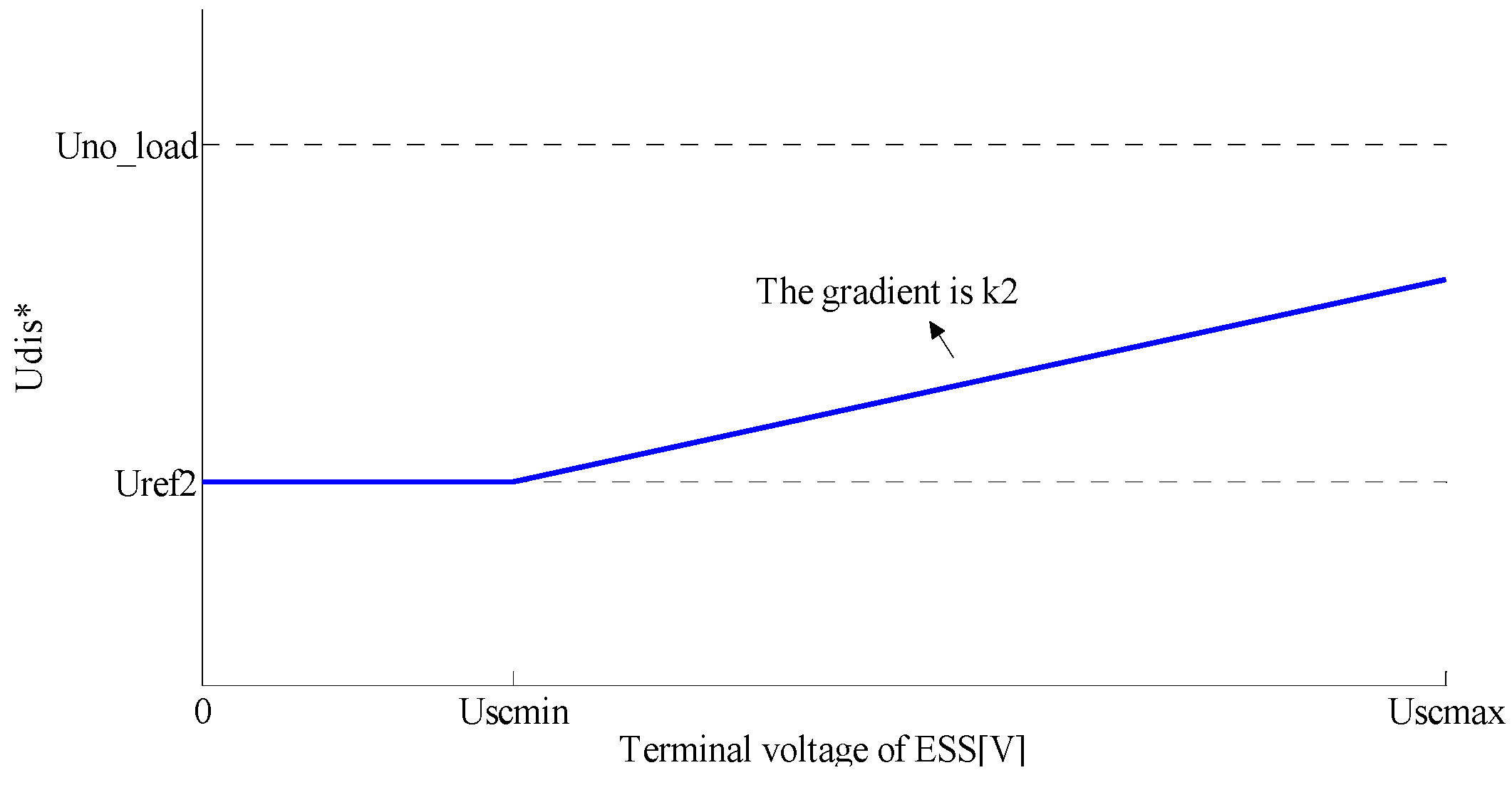
State 3: When the voltage of substation is less than the discharging threshold value U_dis* and pantograph voltage of trains within one substation spacing range of ESS is higher than the low voltage threshold U_low, discharging power reference P_sc* of ESS is determined by the substation voltage U_sub and ESS terminal voltage U_sc simultaneously as follow:

$$\{\begin{array}{l}{P}_{SC}^{*}=K_{p2}\times \left(U_{sub}-U_{dis}^{*}\right)+K_{i2}\times {\displaystyle \underset{0}{\overset{t}{\int }}\left(U_{sub}-U_{dis}^{*}\right)dt}\\ U_{dis}^{*}=U_{ref2}+k_2\times \left(U_{sc}-U_{sc\min }\right)\\ K_{p2}\ge 0,K_{i2}\ge 0,U_{dis}^{*}<U_{no\_load},k_2\ge 0,U_{sc\max }\ge U_{sc}\ge U_{sc\min }\end{array}$$

(18)

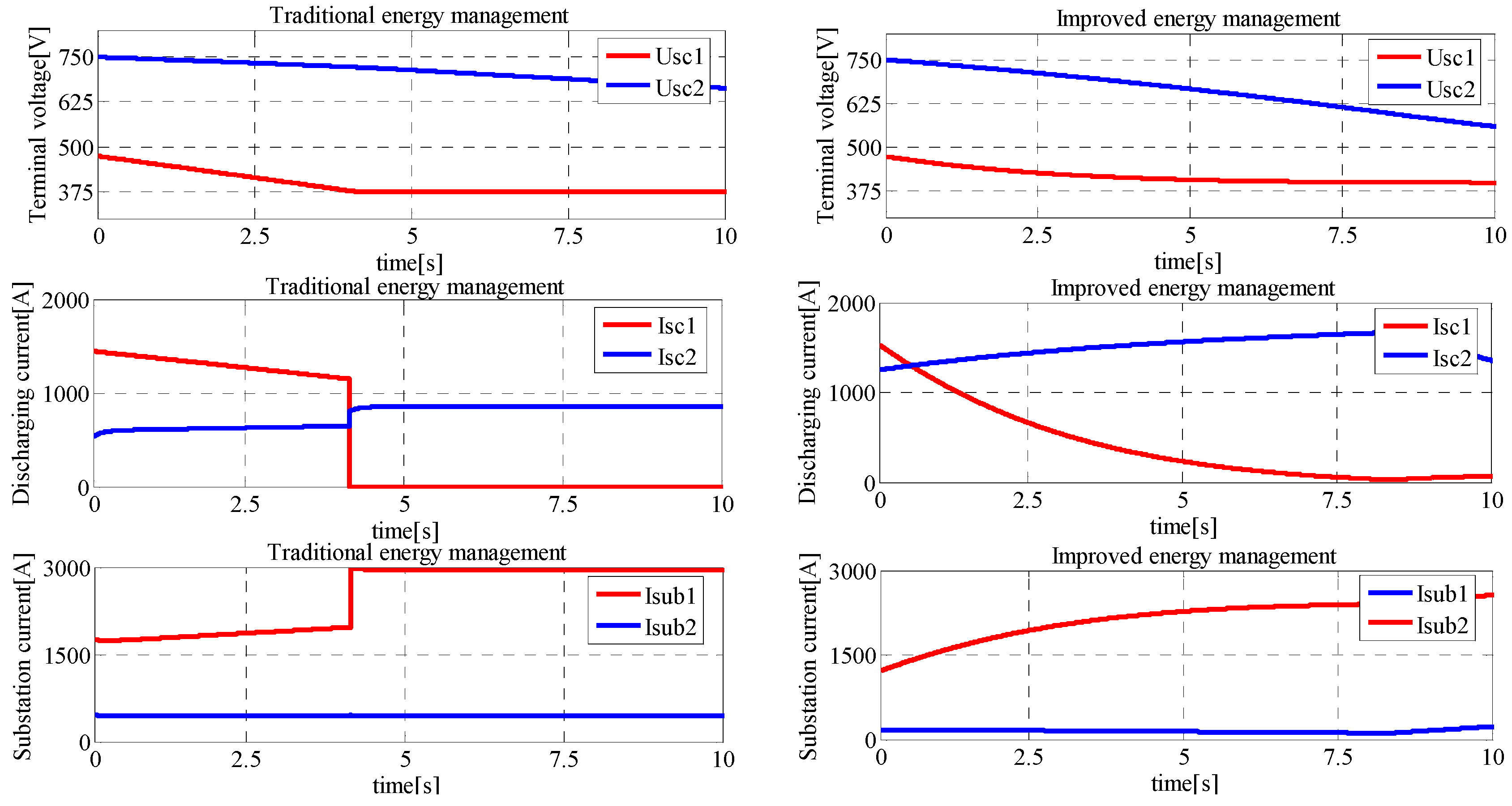
The value of U_dis* will increase with the increase of ESSes’ terminal voltage as shown in Figure 13, which enlarges the discharging current of ESSes with larger terminal voltage and balances SOC of ESSes significantly. When the accelerated train draws the energy in one substation, all ESSes nearby can deliver energy to shave the power of substations and compensate the voltage drops of the pantograph. As shown in Figure 14, by traditional energy management, the ESS installed in the substation will deliver highest power of energy and take no account of its terminal voltage and stored energy. When terminal voltage of one ESS decreases to U_scmin, its discharging current will be interrupted instantaneously, which also leads to drastic changes of substation current and line current. On the contrary, the improved energy management strategy can achieve smoother changes of voltages and currents in the system, and ESSes with higher SOC tend to deliver more energy to the supply network. Thus, by the improved energy management strategy, the flow of energy can be managed more steadily and effectively, and the line loss can be reduced greatly.

State 4: When the voltage of substation is less than discharging threshold value U_dis* and the pantograph voltages of trains within one substation spacing range of ESS are less than the low voltage threshold U_low, super-capacitor ESS will deliver the energy with maximum discharging power. According to appropriate setting of K_p2, K_i2, k₂, U_ref2, U_low, ESS will retain proper energy when the pantograph voltage of a nearby train is acceptable, and when the pantograph voltage of a nearby train is very low, ESS delivers maximum discharging power to shave the peak power of the substation and compensate the pantograph voltage drop.

Figure 13. The values of U_dis^*.

Figure 13. The values of U_dis^*.

Figure 14. Terminal voltage and discharging current of ESSes.

Figure 14. Terminal voltage and discharging current of ESSes.

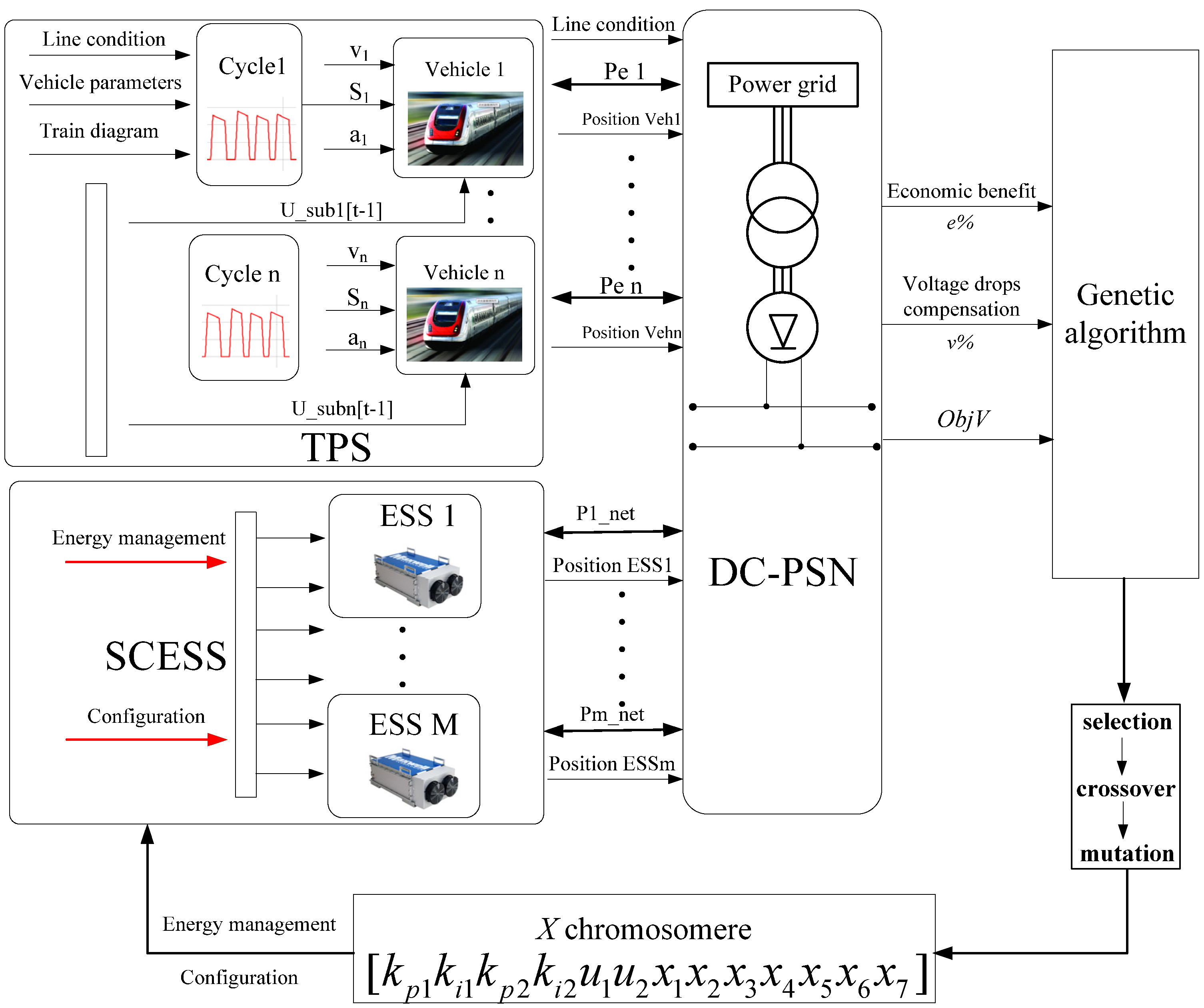
In improved energy management strategy, K_p1, K_i1, k₁, K_p2, K_i2, k₂, U_low, U_ref1, U_ref2 are nine undetermined parameters. In order to obtain best performance of system based on economic efficiency $e\%$ and voltage drop compensation $v\%$, the most appropriate parameters of improved energy management strategy and ESS configuration on each substation will be obtained simultaneously by the optimization method based on a genetic algorithm.

4.2. Novel Optimization Method

4.2.1. Genetic Algorithm

The genetic algorithm (GA) is a global optimal searching algorithm based on Darwin’s nature evolution theory and Mendel’s genetics and mutation theory. It consists of three parts: encoding, fitness evaluation, and genetic manipulation [23,24,25]. Combined with paper demands, the basic procedures of the genetic algorithm are shown as follows.

Encoding

The energy management strategy and configuration of ESSes installed in seven TSSs can be encoded by 16 numbers as shown in Figure 15, where each X chromosomere presents a population individual. The first nine numbers represent nine pending parameters of improved energy management strategy, u₁, u₂, u₃ represent U_low, U_ref1, U_ref2; the last seven numbers represent seven pending numbers of super-capacitor strings installed in seven different traction substations.

Figure 15. Set of X chromosomere.

Figure 15. Set of X chromosomere.

Objective Function ObjV

In this paper, the optimization of energy management strategy and configuration of ESSes is to obtain the maximum objective function ObjV, the reciprocal of ObjV is the value of fitness. They are calculated as follows:

$$\{\begin{array}{c}ObjV[X]=\text{ω}\cdot e\%[X]+(1-\text{ω})\cdot v\%[X]\\ Fitness[X]=\frac{1}{ObjV[X]}\end{array}$$

(19)

where $\text{ω}$ is the weight coefficient of economic efficiency $e\%$. ObjV[X] is the objective function when the energy management strategy, allocation, and size of ESSes are set by X.

Genetic Manipulation

Genetic manipulation includes three basic steps—selection, crossover, and mutation. From the view of operators, the genetic algorithm is well-suited to solve combination optimization problems. Compared with other intelligence algorithms, a genetic algorithm has a higher rate of convergence, more efficient calculation, and higher robustness for combination optimization and discrete optimization.

4.2.2. Process of Novel Optimization Method

The schematic diagram of the novel optimization method, which combines a genetic algorithm and simulation platform of urban rail power supply system, is shown as Figure 16. A genetic algorithm can constantly optimize the chromosomere of the population individuals, which means the energy management strategy and configuration of ESSes are optimized constantly. The newfound energy management strategy and configuration of ESSes would be entered into the simulation platform, and obtain their ObjV, e%, v% through the simulation. According to the ObjV, e%, v%, the genetic algorithm can continue the further and cyclic optimization. According to the optimization results by a large number of simulation calculations, the genetic algorithm converges to the global optimum with the increase of evolution generation.

For every different objective function, the genetic algorithm will take 5.5 days to obtain the corresponding optimal solution. Of course, if several workstations work simultaneously, the total simulation time can be effectively decreased. The simulation platform of urban rail power supply system is established by software Matlab 7.10.0(2010a). The hardware performance of our workstations that implement the simulation platform is shown as Table 5. It is worth mentioning that increasing the population size or improving the genetic algorithm by means of a hybrid algorithm can improve the convergence speed and decrease the evolution generation.

The relevant parameters of the genetic algorithm are given by Table 6; NIND is population size, PRECI is the length of individual, MAXGEN is maximum evolution generation, P_c is the crossover rate, P_m is the mutation rate, and GGAP is generational gap.

Figure 16. The schematic diagram of novel optimization method.

Figure 16. The schematic diagram of novel optimization method.

Table 5. The parameters of hardware platform.

Hardware	Parameter
CPU	Intel(R) Xeon(R) CPU E5649 @ 2.53GHz × 2
RAM	64 GB
GPU	NVIDIA Quadro 4000

Table 5. The parameters of hardware platform.

Hardware	Parameter
CPU	Intel(R) Xeon(R) CPU E5649 @ 2.53GHz × 2
RAM	64 GB
GPU	NVIDIA Quadro 4000

Table 6. The parameters of improved genetic algorithm.

NIND	PRECI	MAXGEN	Pc	Pm	GGAP
40	20	100	0.7	0.015	0.95

Table 6. The parameters of improved genetic algorithm.

NIND	PRECI	MAXGEN	Pc	Pm	GGAP
40	20	100	0.7	0.015	0.95

4.3. Optimization Result Analysis

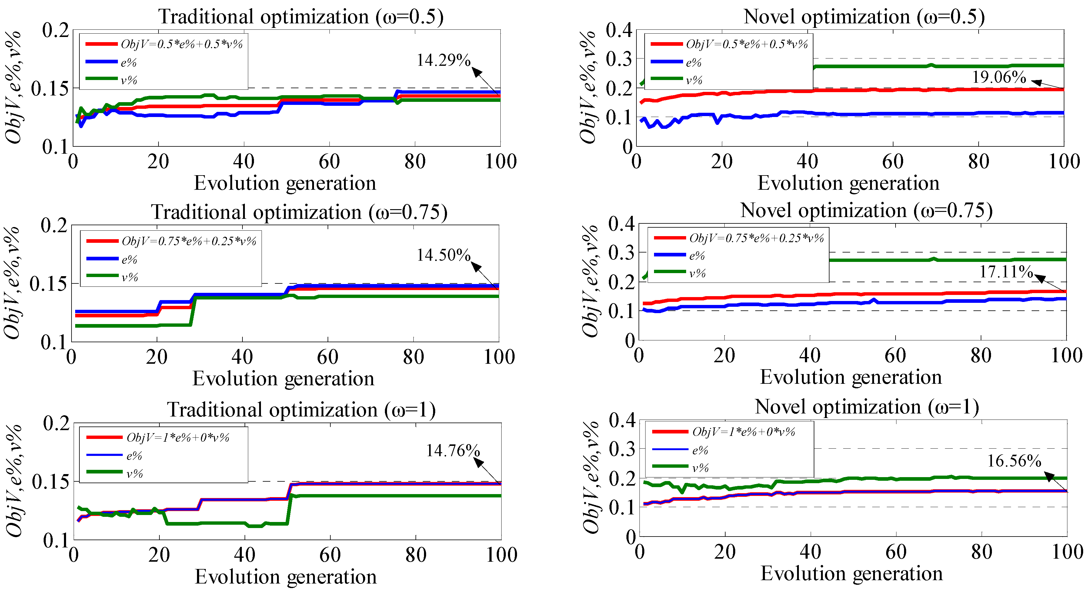
As shown in Figure 17, the simulation comparison result between two different optimization methods with corresponding optimum ObjV are obtained separately under different values of weight coefficient $\omega$. Based on a genetic algorithm, both optimization methods can obtain optimal ObjV with an increase of evolution generation, but the novel optimization method can obtain much higher ObjV. The values of maximum ObjV as well as corresponding economic efficiency $e\%$ and voltage drop compensation, $v\%$ based on two optimization methods and different values of weight coefficient $\omega$ are shown in Table 7. The values of parameters to determine energy management strategy and configuration of ESSes on every substation can be obtained separately based on two optimization methods and different values of weight coefficient $\omega$, as shown in Table 8 and Table 9.

Figure 17. Simulation comparisons of two optimization methods.

Figure 17. Simulation comparisons of two optimization methods.

Table 7. Maximum ObjV obtained by different optimization method.

Optimization Method	ω	Maximum ObjV	Economic Efficiency e%	Voltage Compensation Rate v%
Traditional optimization	0.5	14.29%	14.65%	13.93%
Traditional optimization	0.75	14.50%	14.72%	13.84%
Traditional optimization	1	14.76%	14.76%	13.70%
Novel optimization	0.5	19.06%	15.06%	23.05%
Novel optimization	0.75	17.11%	15.79%	21.06%
Novel optimization	1	16.56%	16.56%	17.20%

Table 7. Maximum ObjV obtained by different optimization method.

Optimization Method	ω	Maximum ObjV	Economic Efficiency e%	Voltage Compensation Rate v%
Traditional optimization	0.5	14.29%	14.65%	13.93%
Traditional optimization	0.75	14.50%	14.72%	13.84%
Traditional optimization	1	14.76%	14.76%	13.70%
Novel optimization	0.5	19.06%	15.06%	23.05%
Novel optimization	0.75	17.11%	15.79%	21.06%
Novel optimization	1	16.56%	16.56%	17.20%

Table 8. The parameters of optimal energy management strategies.

Optimization Method	ω	Energy Management Strategy of ESSes
		kp1	ki1	k1	kp2	ki2	k2	Ulow	Uref1	Uref2
Traditional optimization	-	50	50	-	50	50	-	-	850.0	800.0
Novel optimization	0.5	298	90	0.011	0.158	44.39	0.075	771.0	836.1	802.0
Novel optimization	0.75	193	83	0.006	1.20	40.34	0.037	772.0	836.2	806.4
Novel optimization	1	18	76	0.002	19.33	39.85	0.008	779.1	836.5	811.8

Table 8. The parameters of optimal energy management strategies.

Optimization Method	ω	Energy Management Strategy of ESSes
		kp1	ki1	k1	kp2	ki2	k2	Ulow	Uref1	Uref2
Traditional optimization	-	50	50	-	50	50	-	-	850.0	800.0
Novel optimization	0.5	298	90	0.011	0.158	44.39	0.075	771.0	836.1	802.0
Novel optimization	0.75	193	83	0.006	1.20	40.34	0.037	772.0	836.2	806.4
Novel optimization	1	18	76	0.002	19.33	39.85	0.008	779.1	836.5	811.8

Table 9. Optimized location and size of ESSes.

Optimization Method	ω	TSS No. and Set Numbers of ESSes
		1	2	3	4	5	6	7
Traditional optimization	0.5	0	16	15	0	10	0	13
Traditional optimization	0.75	0	14	15	0	10	0	14
Traditional optimization	1	0	14	15	0	10	0	13
Novel optimization	0.5	0	18	11	0	17	0	17
Novel optimization	0.75	0	18	10	0	10	0	17
Novel optimization	1	0	14	16	0	8	0	7

Table 9. Optimized location and size of ESSes.

Optimization Method	ω	TSS No. and Set Numbers of ESSes
		1	2	3	4	5	6	7
Traditional optimization	0.5	0	16	15	0	10	0	13
Traditional optimization	0.75	0	14	15	0	10	0	14
Traditional optimization	1	0	14	15	0	10	0	13
Novel optimization	0.5	0	18	11	0	17	0	17
Novel optimization	0.75	0	18	10	0	10	0	17
Novel optimization	1	0	14	16	0	8	0	7

From Figure 17 and Table 7, whatever the value of $\text{ω}$, novel optimization method can obtain much higher ObjV, e% and v% compared to traditional optimization method. With the increase of $\text{ω}$ from 0.5 to 0.75 to 1, the maximum ObjV of ESSes obtained by traditional optimization is 14.29%, 14.50%, and 14.76%, which can be increased to 19.06%, 17.11%, and 16.56%, respectively, by the novel optimization method. And both economic efficiency e% and voltage drop compensation v% can be improved effectively by the novel optimization compared to traditional optimization. By the novel optimization method, economic efficiency $e\%$ can be improved because of more appropriate energy management, less line loss, and voltage drop compensation $v\%$ can be improved effectively because of the function of U_low.

From Table 8, the adopted energy management strategy of the traditional optimization method is constant, and it is only determined by six parameters. By contrast, the energy management strategy obtained by the novel optimization method is determined by nine parameters. The novel optimization method can optimize the energy management, location, and size of ESSes simultaneously. Under different values of weight coefficient $\omega$, the best energy management strategy is different and among the nine relevant parameters appear some regularities. k_p1, k₁, k_p2, k₂ are more important factors that affect the performance of the metro system, and k_i1, k_i2, U_low, U_ref1, U_ref2 have smaller changes. 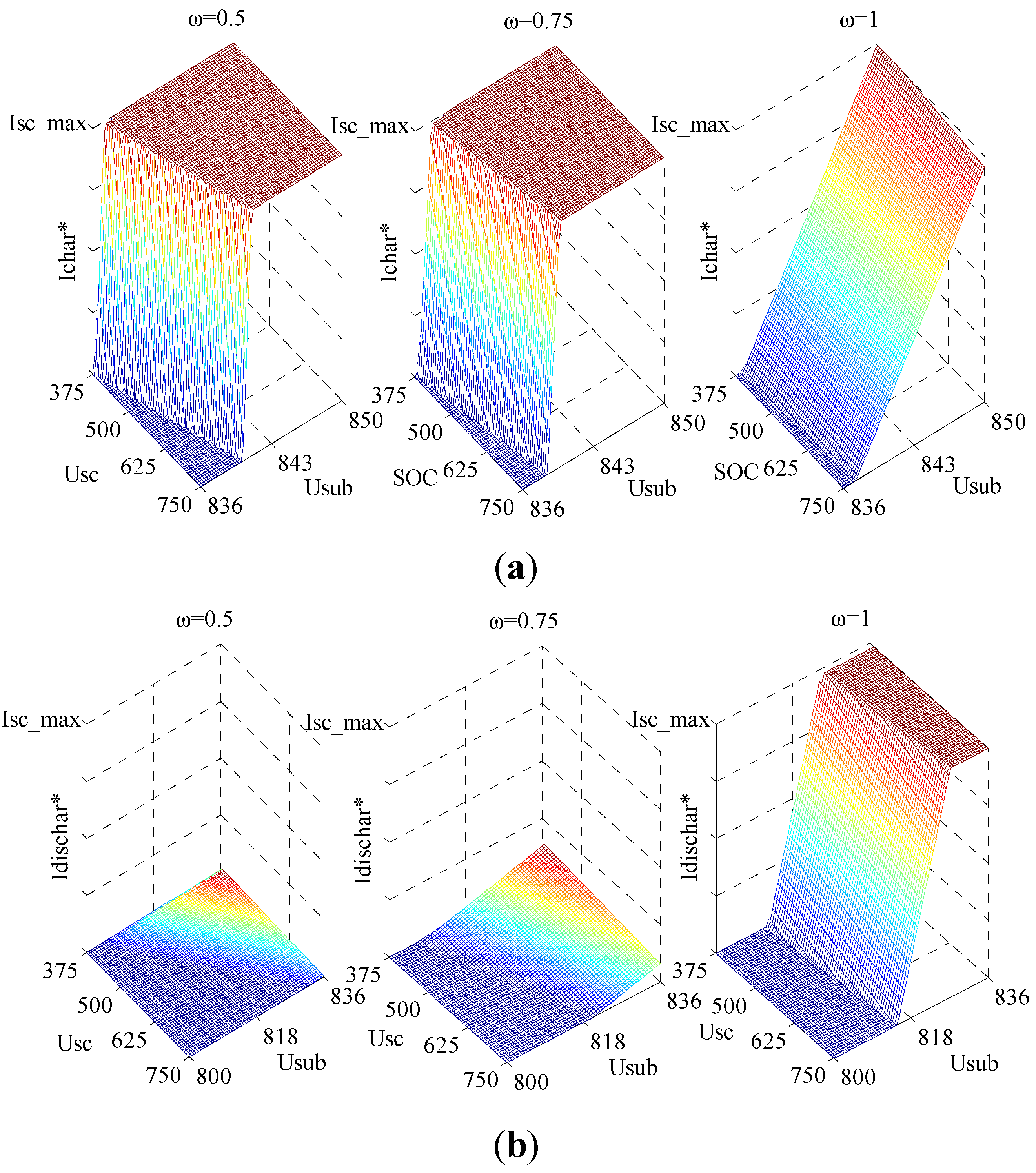Without regard to the integral term, the best energy management strategy of ESSes for different value of weight coefficient $\omega$ is shown in Figure 18. For charging energy management strategy, the value of k_p1 (the slope of charging current vs. U_sub) and k₁ (the slope of charging current vs. U_sc) decrease with the increase of weight coefficient $\omega$. For discharging energy management strategy, the value of k_p2 (the slope of discharging current vs. U_sub) increases and k₂ (the slope of discharging current vs. U_sc) decrease with the increase of weight coefficient $\omega$.

Table 9 shows the optimal location and size of ESSes obtained by two different optimization methods. By contrast, two optimization methods ultimately configure super-capacitor ESSes in same location of substations, and the size of ESSes tend to be smaller with the increase of weight coefficient $\omega$. Configuring ESSes in fewer substations with one or two substation spacing and decreasing the size of ESS installed in one substation can reduce the installation cost, but the distance between the train and ESS will also increase, which causes higher line loss and less energy recovered and voltage drop compensation $v\%$ will also decrease. The best compromise between economic efficiency $e\%$ and voltage drop compensation $v\%$ under different value of weight coefficient $\omega$ can be obtained by two optimization methods. Compared to the traditional optimization method, the best configuration of ESSes obtained by the novel optimization method changes are more intense and it can achieve much higher ObjV under different values of weight coefficient $\omega$.

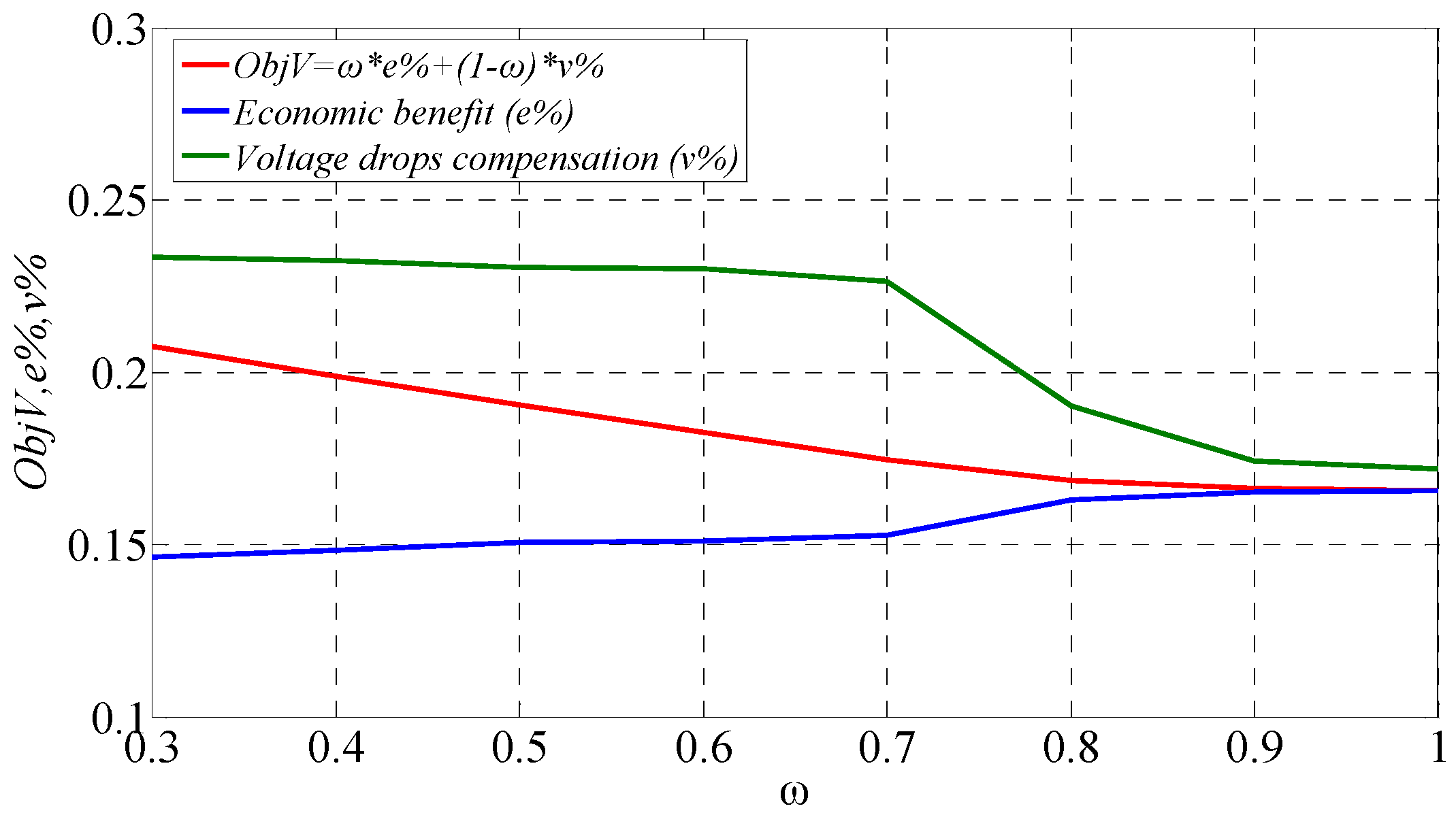
The maximum ObjV with corresponding economic efficiency $e\%$ and voltage drop compensation $v\%$ for different value of weight coefficient $\omega$ can be obtained by novel optimization method as shown in Table 10 and Figure 19. From Figure 19, when $\omega$ increases from 0.3 to 1, Economic efficiency $e\%$ increases from 0.1465 to 0.1656, and voltage drop compensation $v\%$ decreases from 0.2335 to 0.1720. According to its own optimization requirement and the concrete result obtained by the novel optimization method in Figure 19, Subway Company could choose the best value of weight coefficient $\omega$ for itself.

Figure 18. Best energy management strategy of ESSes. (a) Charging energy management strategy; and (b) discharging energy management strategy.

Figure 18. Best energy management strategy of ESSes. (a) Charging energy management strategy; and (b) discharging energy management strategy.

Table 10. Optimal ObjV, e% and v% obtained by novel optimization method.

$\omega$	0.3	0.4	0.5	0.6	0.7	0.8	0.9	1
ObjV	0.2074	0.1989	0.1906	0.1826	0.1747	0.1685	0.1663	0.1656
e%	0.1465	0.1485	0.1506	0.1509	0.1525	0.1631	0.1654	0.1656
v%	0.2335	0.2325	0.2305	0.2301	0.2265	0.1902	0.1744	0.1720

Table 10. Optimal ObjV, e% and v% obtained by novel optimization method.

$\omega$	0.3	0.4	0.5	0.6	0.7	0.8	0.9	1
ObjV	0.2074	0.1989	0.1906	0.1826	0.1747	0.1685	0.1663	0.1656
e%	0.1465	0.1485	0.1506	0.1509	0.1525	0.1631	0.1654	0.1656
v%	0.2335	0.2325	0.2305	0.2301	0.2265	0.1902	0.1744	0.1720

Figure 19. Optimal ObjV, e% and v% obtained by the novel optimization method.

Figure 19. Optimal ObjV, e% and v% obtained by the novel optimization method.

5. Conclusions

Firstly, this paper establishes the proper simulation platform of a metro system that contains seven substations to simulate the electrical power flow by Matlab/Simulink. Then, two evaluation functions are set up from the perspectives of economic efficiency and voltage drop compensation. Ultimately, a novel optimization method is put forward, which can optimize the energy management strategy, location, and size of ESSes simultaneously by the combination of a genetic algorithm and simulation platform of a metro system. With actual parameters of a Chinese metro line applied in the simulation comparison, the proposed novel optimization method can achieve much better performance of a metro system from the perspectives of ObjV and two evaluation functions. The simulation result obtained by the novel optimization method shows that with the increase of weight coefficient $\omega$, the optimal energy management strategy is different and the nine relevant parameters appear with some regularities, among them k_p1, k₁, k_p2, and k₂ are more important factors that affect the performance of the metro system. Additionally, novel optimization methods can also optimize the configuration of ESSes, which can achieve the best compromise between economic efficiency $e\%$ and voltage drop compensation $v\%$. The novel optimization method and its optimized result can provide valuable reference to Subway Company.