An Analysis of Variable-Speed Wind Turbine Power-Control Methods with Fluctuating Wind Speed


Abstract
:1. Introduction
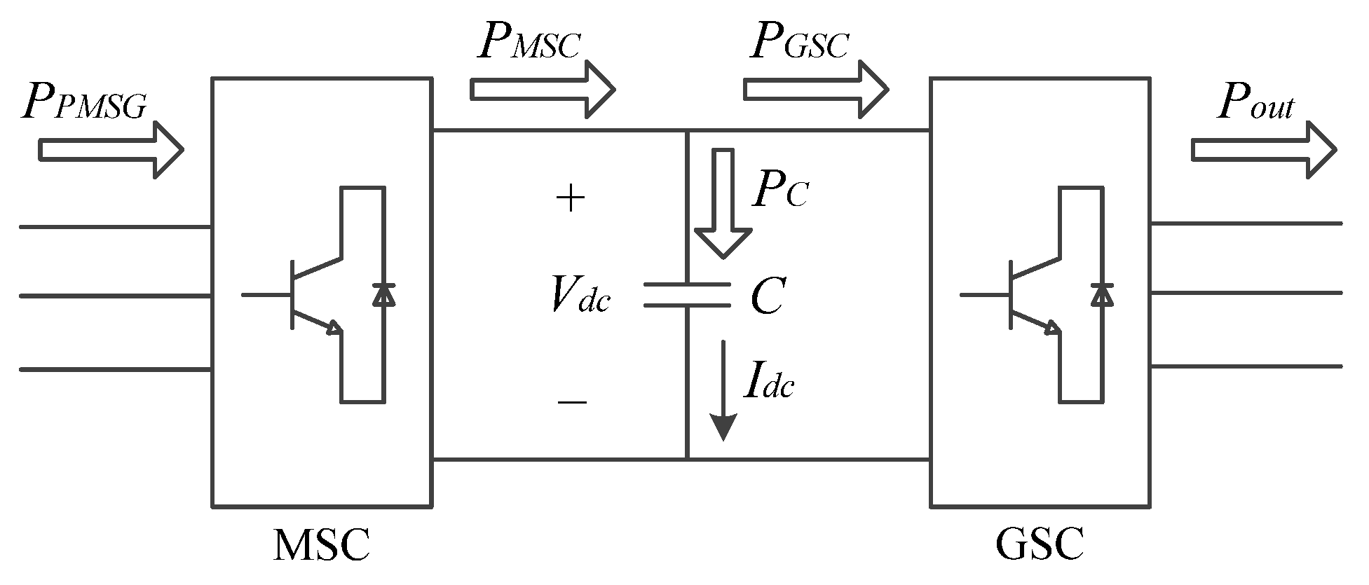
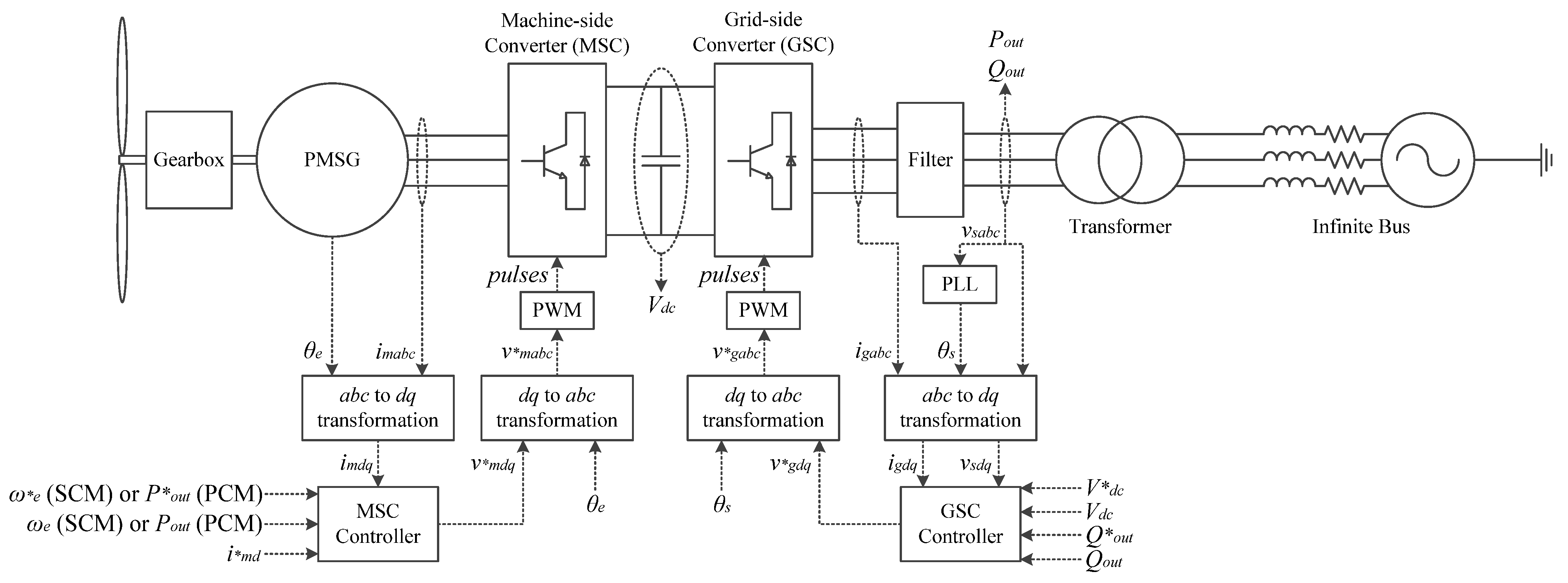
2. Wind Energy Conversion System

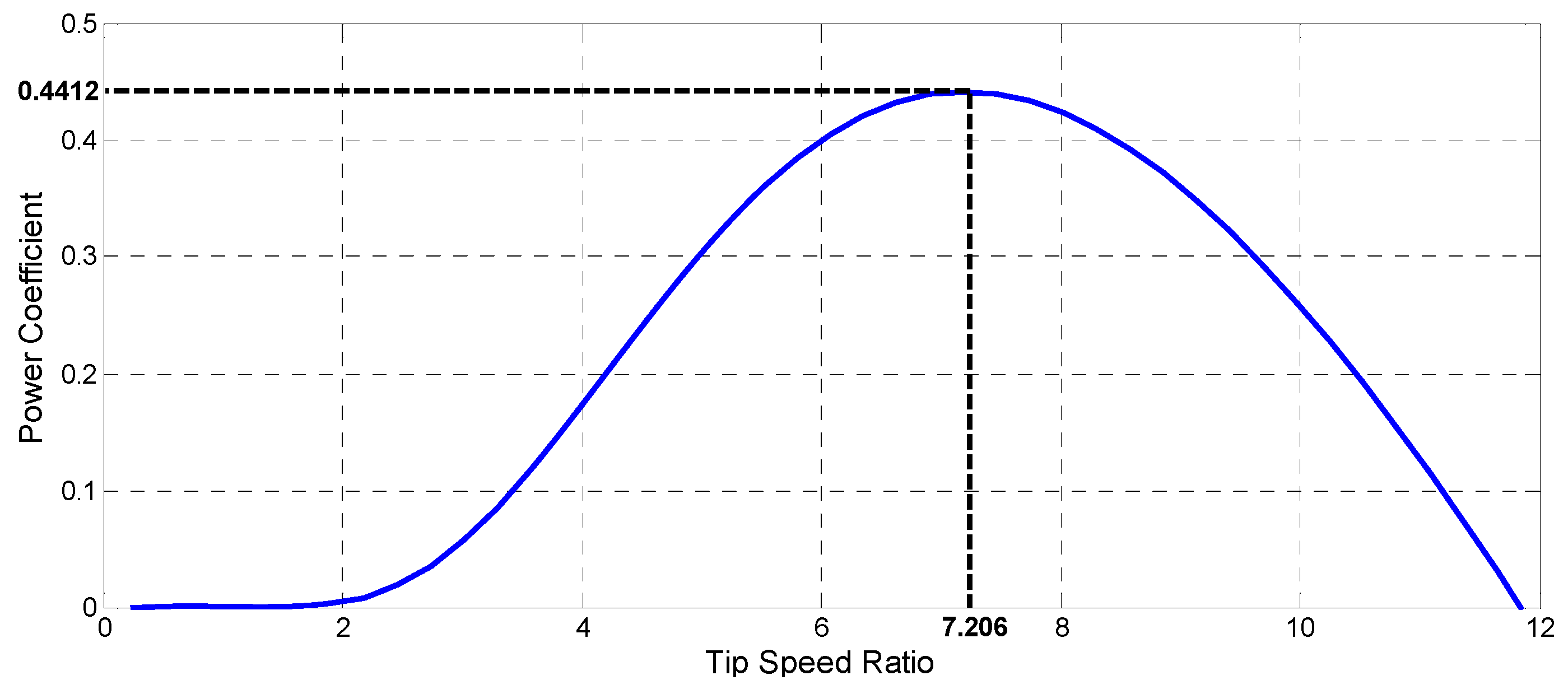
2.1. Wind Turbine Model

2.2. PMSG Model
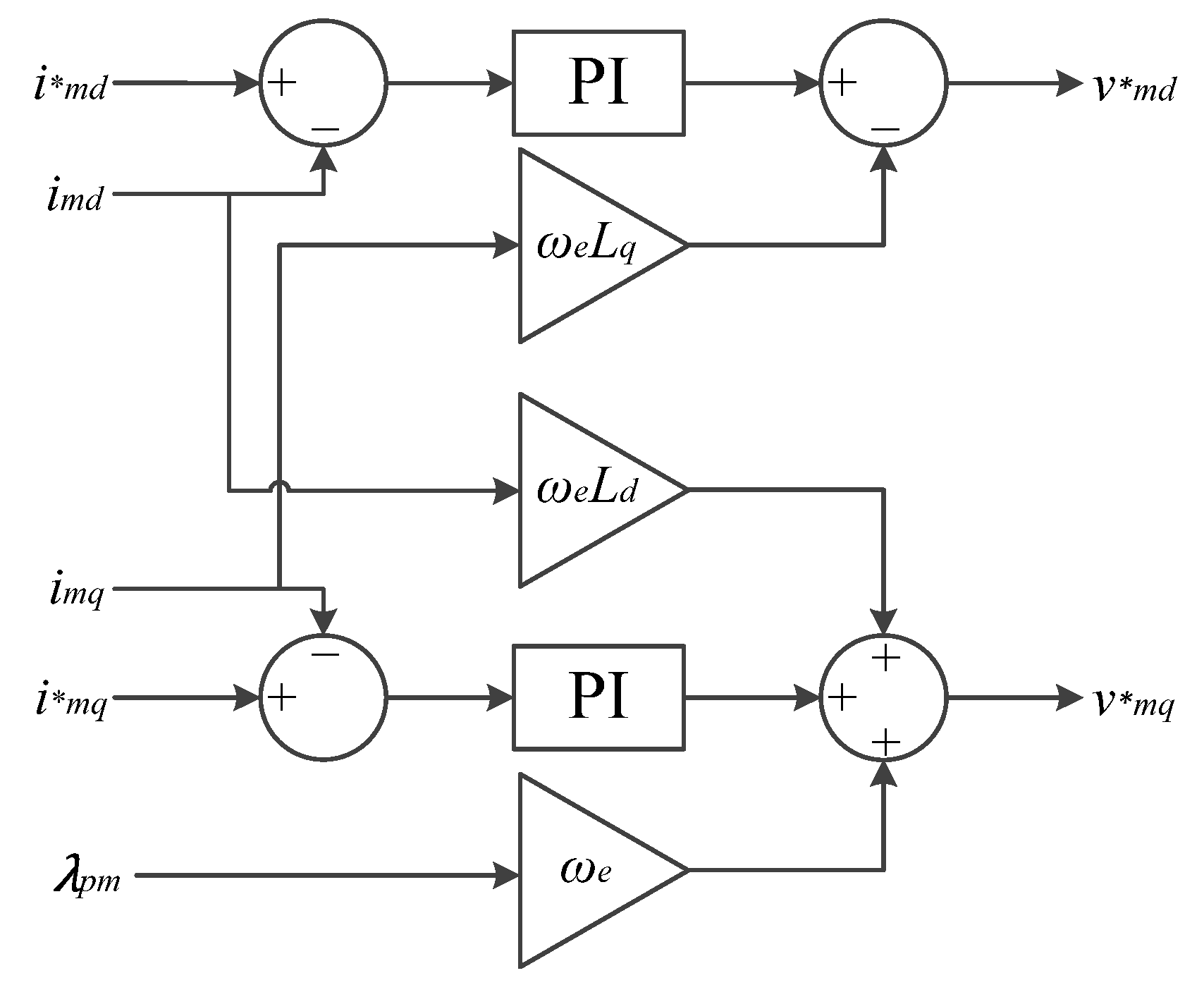
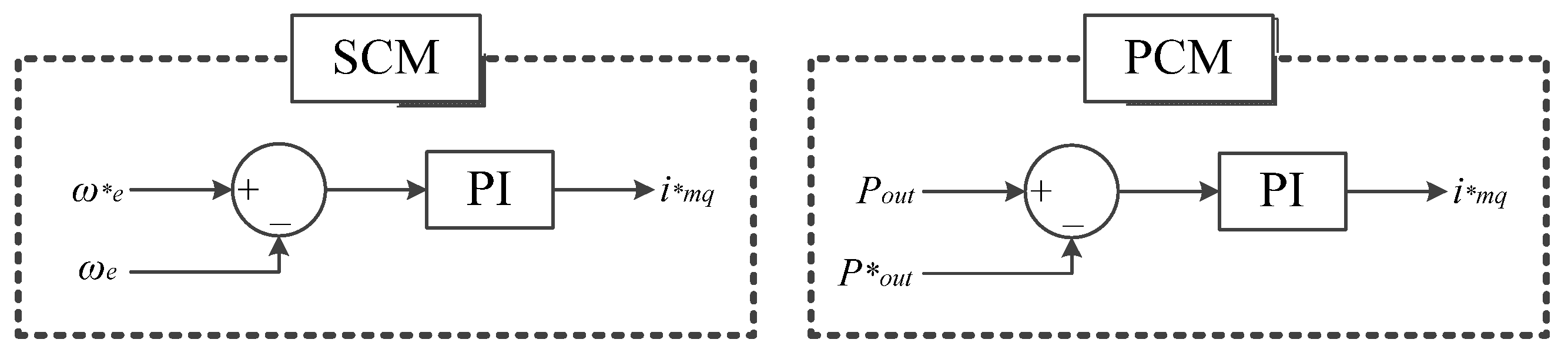
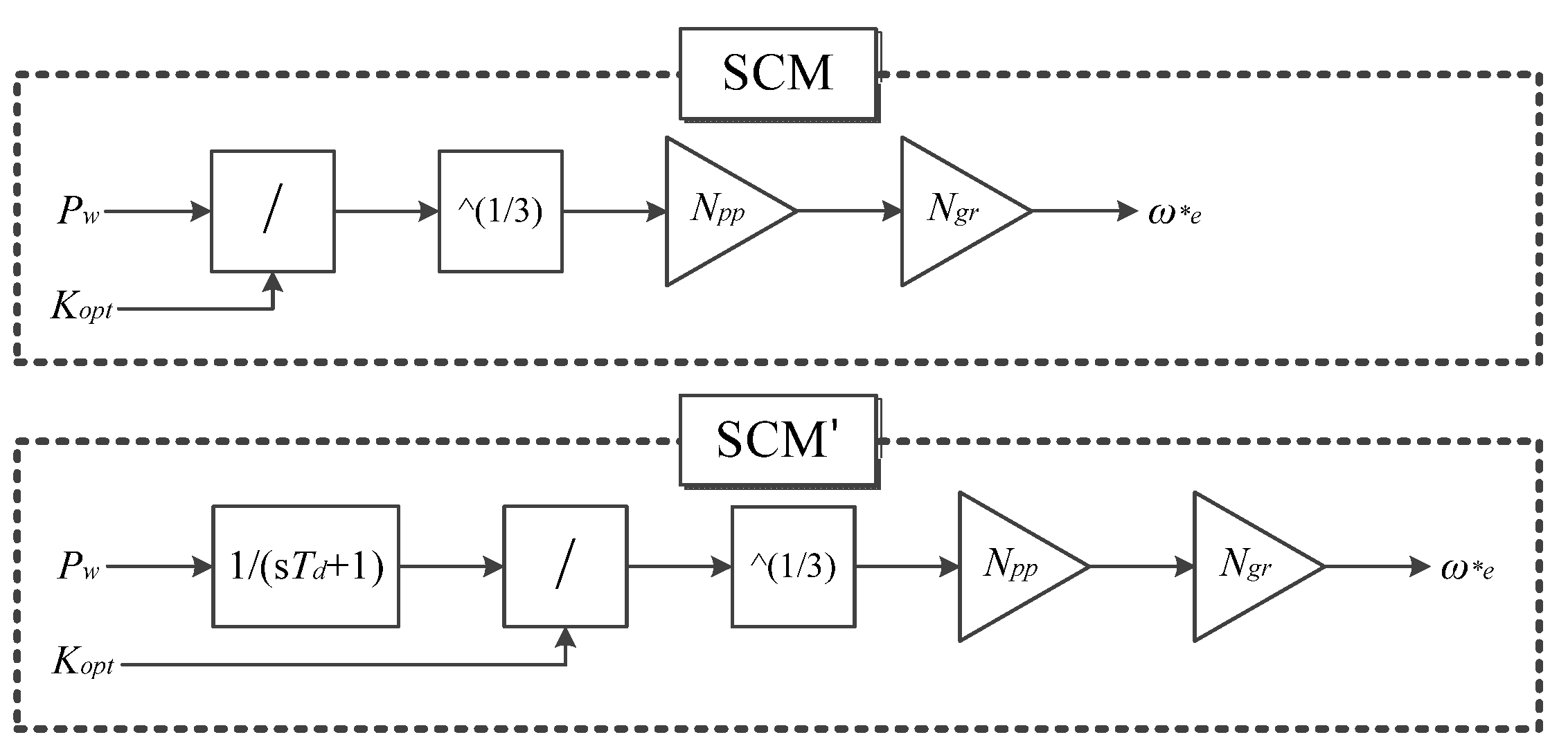
2.3. Machine-Side Converter Control
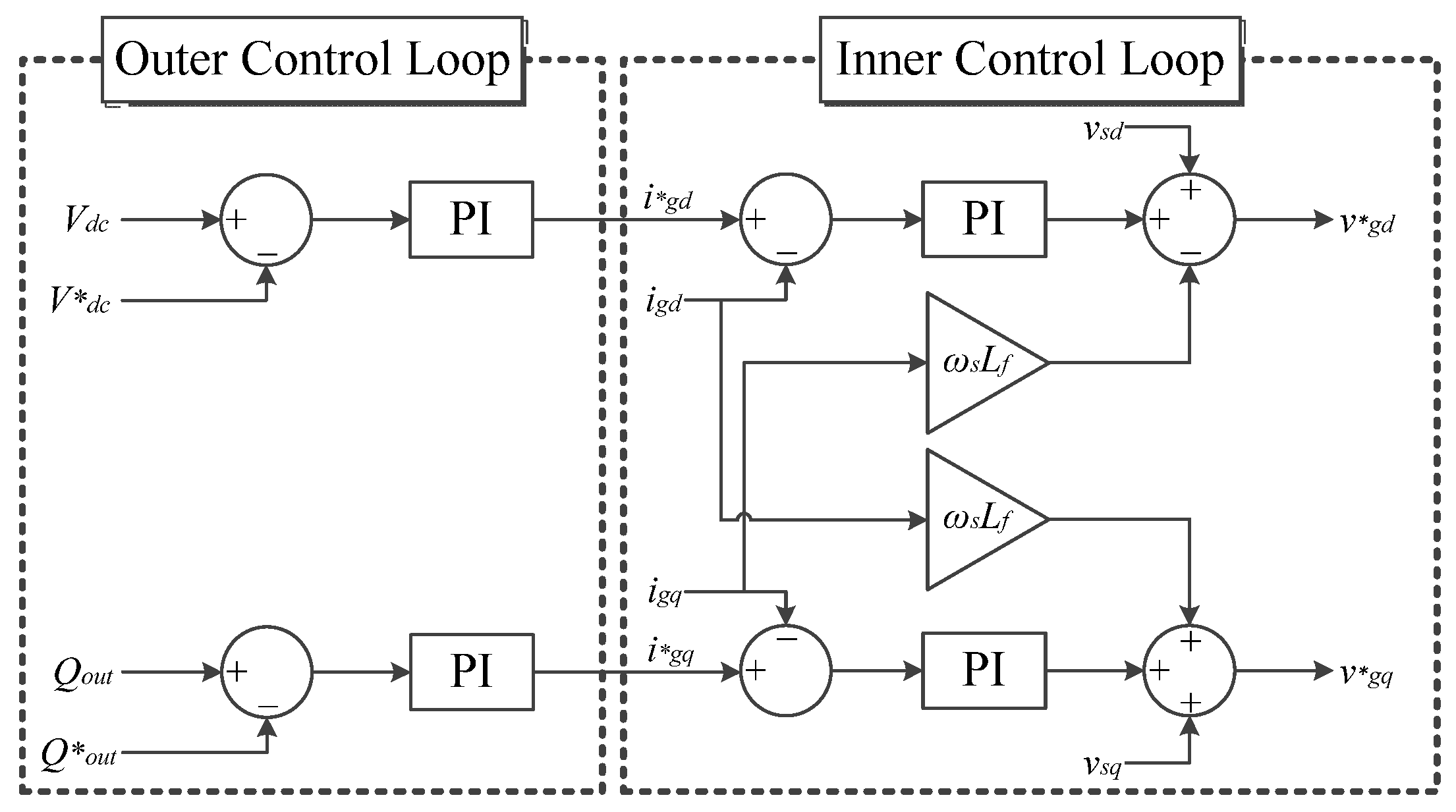
2.4. Grid-Side Converter Control
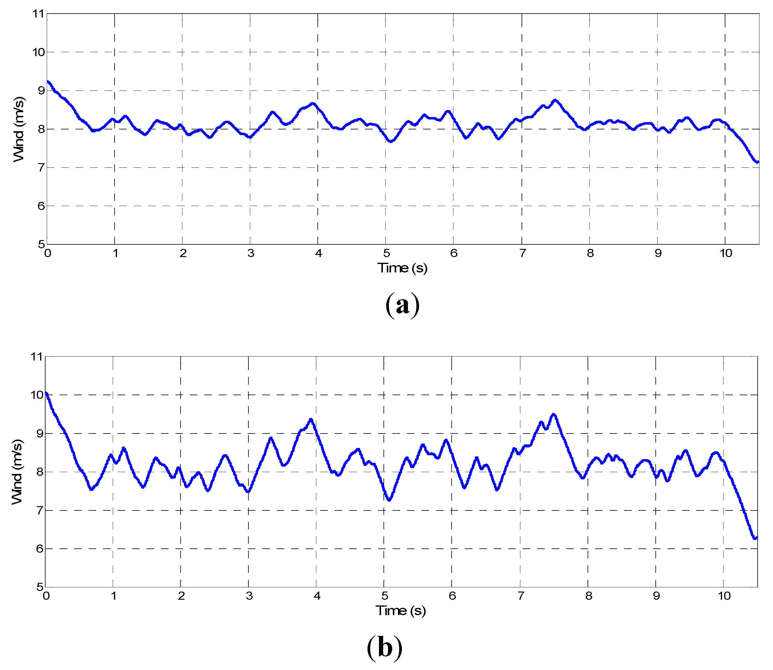
3. Case Study

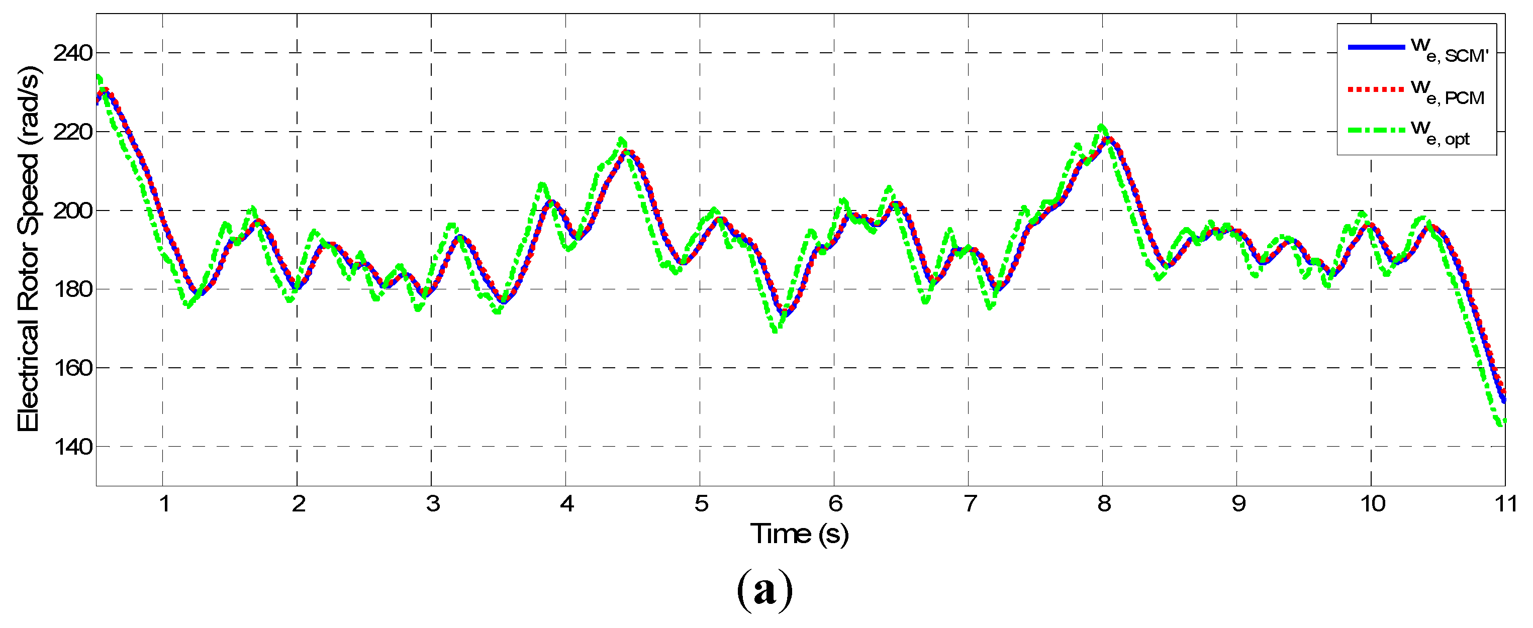
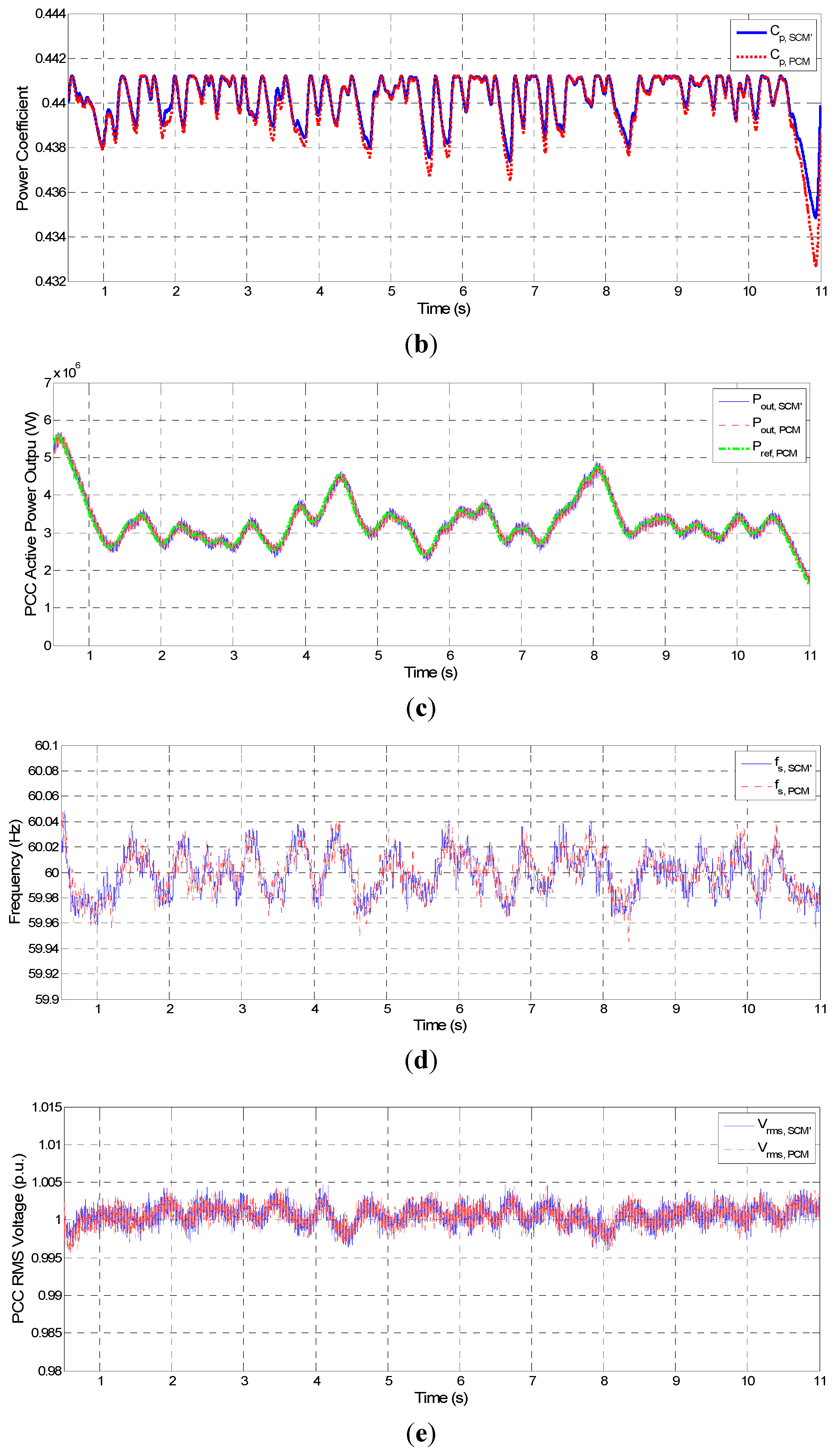
3.1. Simulation Results

| Parameters | Value | Unit |
|---|---|---|
| Rated power | 7.35 | MW |
| Rotor radius | 83.5 | m |
| Nominal wind turbine rotor speed | 0.936 | rad/s |
| Gearbox ratio | 30 | - |
| Number of pole pairs | 9 | - |
| Parameters | Value | Unit |
|---|---|---|
| Nominal power | 7.35 | MVA |
| Nominal primary/secondary voltage | 3.3/22.9 | kV |
| Primary and secondary resistance/inductance | 0.002/0.08 | p.u. |
| Parameters | Value | Unit |
|---|---|---|
| 3-phase short-circuit level at base voltage | 100 | MVA |
| Base voltage | 22.9 | kV |
| X/R ratio | 7 | - |
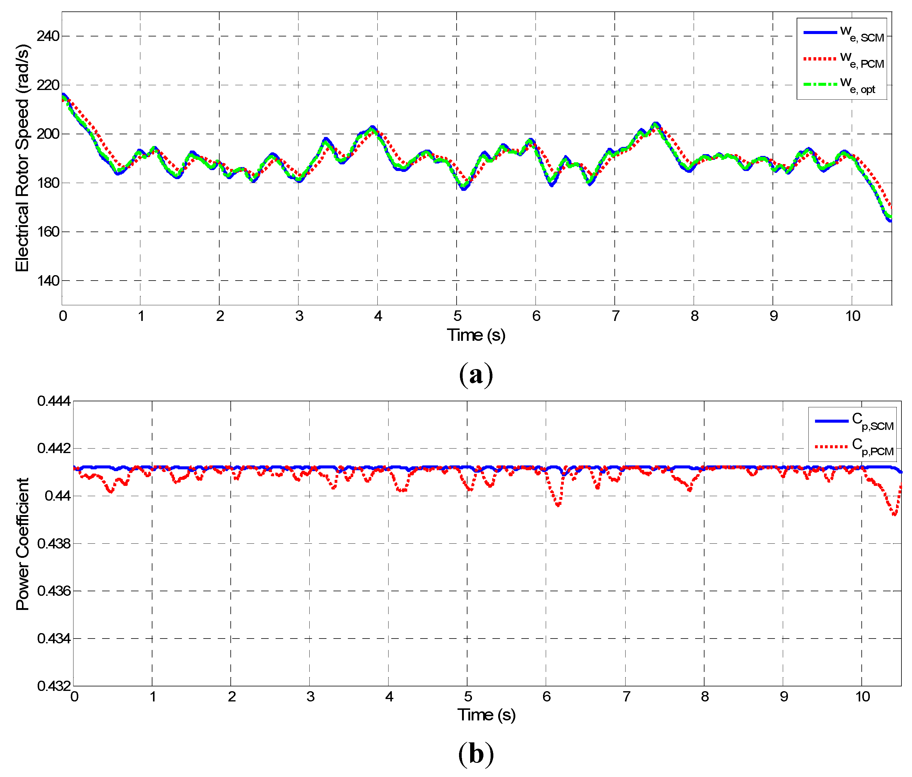
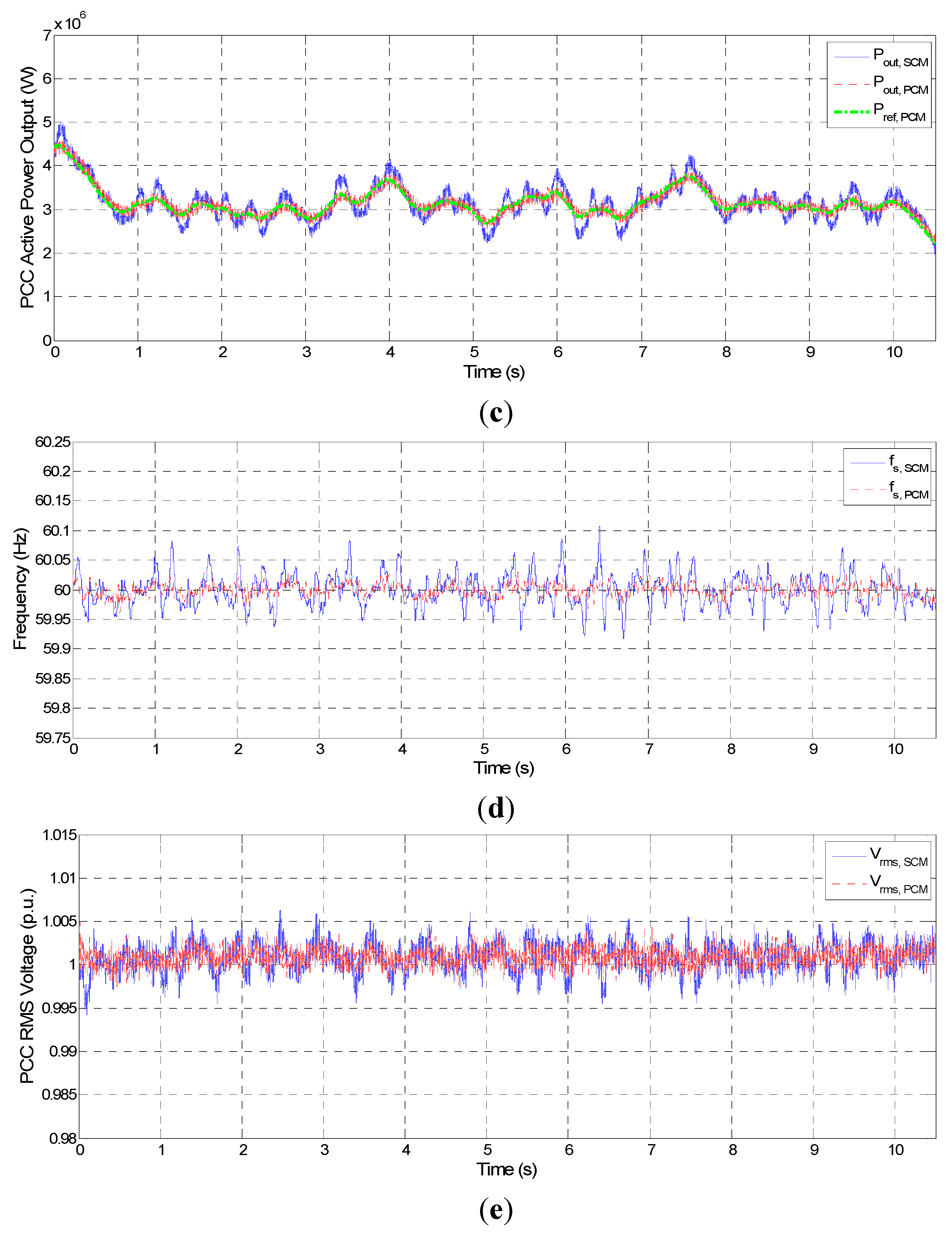
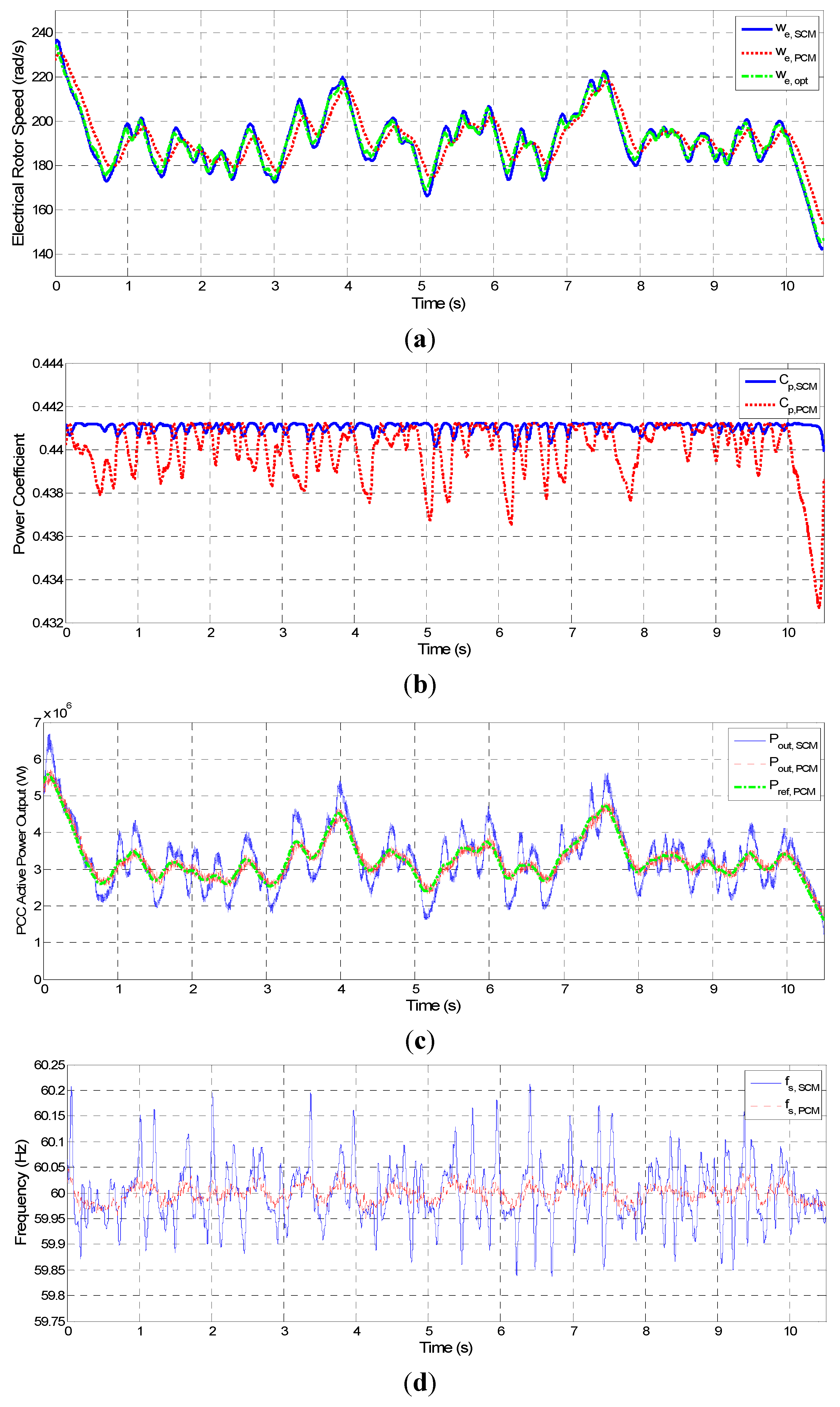
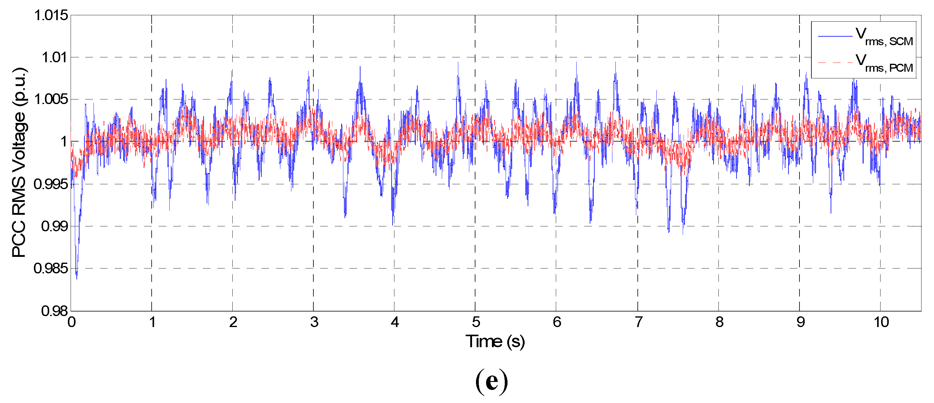
3.2. Discussion
| Control Mode | Case 1 | Case 2 | ||
|---|---|---|---|---|
| SCM | 0.4412 | 0.0003 | 0.4410 | 0.0012 |
| PCM | 0.4409 | 0.002 | 0.4400 | 0.0085 |
| Control Mode | Case 1 (Hz) | Case 2 (Hz) | ||||
|---|---|---|---|---|---|---|
| SCM | 59.9170 | 60.1070 | 0.1070 | 59.8377 | 60.2199 | 0.2199 |
| PCM | 59.9613 | 60.0301 | 0.0387 | 59.9457 | 60.0469 | 0.0543 |
| Control Mode | Case 1 (p.u.) | Case 2 (p.u.) | ||||
|---|---|---|---|---|---|---|
| SCM | 0.9942 | 1.0063 | 0.0063 | 0.9838 | 1.0095 | 0.0162 |
| PCM | 0.9974 | 1.0050 | 0.0050 | 0.9958 | 1.0045 | 0.0045 |

4. Conclusions
Acknowledgments
Conflict of Interest
References
- Global Wind Energy Council. Global Wind Energy Outlook 2012; Global Wind Energy Council: Brussels, Belgium, 2012. Available online: http://www.gwec.net/wp-content/uploads/2012/11/GWEO_2012_lowRes.pdf (accessed on 5 June 2013).
- Iglesias, R.L.; Arantegui, R.L.; Alonso, M.A. Power electronics evolution in wind turbines—A market-based analysis. Renew. Sustain. Energy Rev. 2011, 15, 4982–4993. [Google Scholar] [CrossRef]
- Ackermann, T. Wind Power in Power Systems; John Wiley & Sons: Hoboken, NJ, USA, 2005. [Google Scholar]
- Tsili, M.A.; Papathanassiou, S.A. A review of grid code technical requirements for wind farms. IET Renew. Power Gener. 2009, 3, 308–332. [Google Scholar] [CrossRef]
- Teodorescu, R.; Liserre, M.; Rodríguez, P. Grid Converters for Photovoltaic and Wind Power Systems; John Wiley & Sons: Hoboken, NJ, USA, 2011. [Google Scholar]
- Uehara, A.; Pratap, A.; Goya, T.; Senjyu, T.; Yona, A.; Urasaki, N.; Funabashi, T. A coordinated control method to smooth wind power fluctuations of a PMSG-based WECS. IEEE Trans. Energy Convers. 2011, 26, 550–558. [Google Scholar] [CrossRef]
- Qu, L.; Qiao, W. Constant power control of DFIG wind turbines with supercapacitor energy storage. IEEE Trans. Ind. Appl. 2011, 47, 359–367. [Google Scholar] [CrossRef]
- Teleke, S.; Baran, M.E.; Huang, A.Q.; Bhattacharya, S.; Anderson, L. Control strategies for battery energy storage for wind farm dispatching. IEEE Trans. Energy Convers. 2009, 24, 725–732. [Google Scholar] [CrossRef]
- Morren, J.; de Haan, S.W.H.; Kling, W.L.; Ferreira, J.A. Wind turbines emulating inertia and supporting primary frequency control. IEEE Trans. Power Syst. 2006, 21, 433–434. [Google Scholar] [CrossRef]
- Conroy, J.F.; Watson, R. Frequency response capability of full converter wind turbine generators in comparison to conventional generation. IEEE Trans. Power Syst. 2008, 23, 649–656. [Google Scholar] [CrossRef]
- Chang-Chien, L.R.; Lin, W.T.; Yin, Y.C. Enhancing frequency response control by DFIGs in the high wind penetrated power systems. IEEE Trans. Power Syst. 2011, 26, 710–718. [Google Scholar] [CrossRef]
- Wang, X.; Wu, S. Nonlinear Dynamic Modeling and Numerical Simulation of the Wind Turbine’s Gear Train. In Proceedings of the 2011 International Conference on Electrical and Control Engineering, Yichang, China, 16 September–18 September 2011; pp. 2385–2389.
- Chang-Chien, L.R.; Yin, Y.C. Strategies for operating wind power in a similar manner of conventional power plant. IEEE Trans. Energy Convers. 2009, 24, 926–934. [Google Scholar] [CrossRef]
- Luo, C.; Bankar, H.; Shen, B.; Ooi, B.T. Strategies to smooth wind power fluctuations of wind turbine generator. IEEE Trans. Energy Convers. 2007, 22, 341–349. [Google Scholar] [CrossRef]
- Morren, J.; Pierik, J.; de Haan, S.W.H. Inertial response of variable speed wind turbines. Electr. Power Syst. Res. 2006, 76, 980–987. [Google Scholar] [CrossRef]
- Bankar, H.; Luo, C.; Ooi, B.T. Steady-state stability analysis of doubly-fed induction generators under decoupled P-Q control. IEE Proc. Electr. Power Appl. 2006, 153, 300–306. [Google Scholar] [CrossRef]
- Yazdani, A.; Iravani, R. A neutral-point clamped converter system for direct-drive variable-speed wind power unit. IEEE Trans. Energy Convers. 2006, 21, 596–607. [Google Scholar] [CrossRef]
© 2013 by the authors; licensee MDPI, Basel, Switzerland. This article is an open access article distributed under the terms and conditions of the Creative Commons Attribution license (http://creativecommons.org/licenses/by/3.0/).
Share and Cite
Kim, Y.-S.; Chung, I.-Y.; Moon, S.-I. An Analysis of Variable-Speed Wind Turbine Power-Control Methods with Fluctuating Wind Speed. Energies 2013, 6, 3323-3338. https://doi.org/10.3390/en6073323
Kim Y-S, Chung I-Y, Moon S-I. An Analysis of Variable-Speed Wind Turbine Power-Control Methods with Fluctuating Wind Speed. Energies. 2013; 6(7):3323-3338. https://doi.org/10.3390/en6073323
Chicago/Turabian StyleKim, Yun-Su, Il-Yop Chung, and Seung-Il Moon. 2013. "An Analysis of Variable-Speed Wind Turbine Power-Control Methods with Fluctuating Wind Speed" Energies 6, no. 7: 3323-3338. https://doi.org/10.3390/en6073323
APA StyleKim, Y.-S., Chung, I.-Y., & Moon, S.-I. (2013). An Analysis of Variable-Speed Wind Turbine Power-Control Methods with Fluctuating Wind Speed. Energies, 6(7), 3323-3338. https://doi.org/10.3390/en6073323