Fast Explicit Formulations of Propane Thermophysical Properties for Dynamic Modelling

Abstract

While traditional equations of state can determine thermophysical properties, they are computationally demanding, as most formulations are implicit and require iterative solutions. Dynamic simulation of complex energy systems involves various components defined by mathematical equations. Incorporating equations of state for refrigerant properties adds complexity, slowing down the computation. Moreover, studies have demonstrated that calculations of refrigerant thermophysical properties have the most significant impact on computational speed. Therefore, this work develops fast, accurate, and explicit thermodynamic formulations for thermophysical properties of propane, a widely used natural refrigerant for the new generation of heat pumps. The developed set of formulations yielded a mean absolute relative deviation of less than 1% for most of the formulations across the saturated lines and the different phase regions. The results show that using the explicit formulations for dynamic simulation of an air-source heat pump cycle achieves up to a 117× speedup compared to CoolProp, with a maximum relative error around 1% for the COP. This level of accuracy is suitable for applications such as vapor-compression cycle simulations, where accuracy is sacrificed in favor of computational speed. In addition, they offer greater flexibility for modelling and optimizing complex energy systems.

1. Introduction

Heat pumps are recognized as a key technology for the decarbonization of heating and cooling, offering a highly efficient alternative to conventional fossil-fuel-based equipment. Their importance is particularly evident in residential applications, where a substantial share of energy consumption is associated with the heating demand. This technological shift is underscored by the fact that both heating and cooling account for 50% of the European Union’s final energy consumption [1] and contribute 17.5% of global greenhouse gas emissions [2]. Consequently, accelerating the deployment of heat pumps is essential for reducing energy consumption and achieving emissions reductions across the residential sector.

The efficiency of a heat pump is affected by the thermophysical properties of the refrigerant used. An ideal refrigerant for heat pump applications should possess a high critical temperature, a low freezing point, and a high specific enthalpy of vaporization to ensure efficient system operation [3]. Traditional halogenated hydrocarbons, such as R32 and R404A, have been widely used as refrigerants in heat pumps; however, due to their environmental impacts, natural hydrocarbons are being investigated as sustainable alternatives [4]. These natural hydrocarbons offer favourable thermophysical properties, a low global warming potential, and zero ozone-depleting potential. Among the natural refrigerants, propane has been identified as an alternative for residential applications because it is highly energy-efficient and entirely F-gas-free [5]. Additionally, some studies showed that propane outperforms with an efficiency exceeding 10% compared to both R134a and the hydrofluoroolefin R1234yf when tested in a 5.6 kW brine-to-water heat pump for the residential sector [6].

Accurate knowledge of refrigerant thermophysical properties is essential for simulating vapor-compression cycles. These cycles can take hours/days for simulation, especially if they include strong dynamic behaviour or discretized heat exchanger models [7]. For example, Zhao et al. [8] reported that more than 10 h are needed to simulate a three-dimensional fin-and-tube heat exchanger using REFPROP [9]. Consequently, any optimization performed on such simulation software could take months or even years, as reported by Zhao [8].

Refrigerant thermophysical properties can be determined using an appropriate equation of state (EOS) [10]. Various EOS formulations have been developed for different refrigerants. The NIST REFPROP [11] and CoolProp [12] libraries are both widely accepted sources for such EOS and for the calculation of thermophysical properties. In both packages, propane thermodynamic properties are primarily derived from the Helmholtz-energy-based EOS [13]. These external libraries demonstrate relatively slow computational performance in thermophysical property calculations. This is primarily due to the complexity of the implicit multi-variable differential formulations, which use temperature and density as input variables. In contrast, most numerical models of energy systems employ pressure and enthalpy. Consequently, internal iterations are necessary when using the Helmholtz EOS.

One of the earliest studies addressing improvements in thermophysical property calculations was conducted by Cleland in 1986 [14] and later extended in 1994 [15]. Cleland proposed explicit-based formulations for calculating saturated liquid and vapor properties, such as enthalpy and density. The proposed equations with polynomial terms are 20 times faster than those with exponential terms. Ding et al. [16] proposed an implicit formulation for refrigerant property calculations and demonstrated its application to R22 and R407C. They reported speed-up factors up to 1000 compared with REFPROP [16]. Afterwards, Ding highlighted key requirements for reliable vapor compression system simulations, including speed, stability, reversibility, and continuity [17]. Here, “reversibility” refers strictly to its mathematical definition and is unrelated to thermodynamic reversibility or entropy generation. Additionally, they also showed that the calculation speed of R410A formulae is 100 times faster than that of REFPROP [8]. On the other hand, Kunick et al. developed a spline-based table look-up (SBTL) method that maintains high accuracy and consistency while being significantly faster than REFPROP, achieving a speed-up factor of 225 [18]. The SBTL is then implemented by Li et al. in Dymola, demonstrating significant computational speedups of 2–4× across a range of complex air conditioning system models [19]. As an example of a hybrid approach, Sieres et al. presented a method combining the implicit formulations of Ding et al. [16,17] with their proposed explicit formulations, which are derived for specific properties only [20]. Moreover, they reported detailed accuracy metrics, such as a mean percentage deviation of 7 × 10⁻³ for R407C temperature predictions in the two-phase region, but no computational speed was provided. Afterwards, Aute and Radermacher proposed a rational polynomial functional form to represent all thermophysical properties as functions of saturation pressure, resulting in linear regression forms that are easy to implement [21]. They also reported speed-up factors of 119 and 646 in the heat exchanger simulations for R407F and R404A, respectively. Finally, Khoury et al. compared their work using the implicit fitting method with CoolProp for a complex cascade refrigeration cycle in Dymola [7]. In addition to the high accuracy, they reported a 30× speedup in the simulation over CoolProp.

Although some studies have suggested that their approaches can be extended to other refrigerants (for instance, Sieres investigated two refrigerants, with seven additional ones included in the supplementary data [20], and Khoury demonstrated a cascade refrigeration cycle using three different refrigerants [7]), propane has not yet been examined. Additionally, the implicit methods proposed by both Sieres and Khoury face two main challenges: identification of the correct physical solution and irreversibility. The former requires additional calibrations and equation constraints to select the correct physical solution among the three possible roots of the equation. Irreversibility can be explained as follows: for a formulation to be reversible, if an initial input parameter is used to compute an output parameter through an explicit expression, then using this output as the input to another explicit expression should reproduce the original input value. This concept is illustrated in Figure 1, where two pressure values ($p_A$ and $p_B$) yield a single value of the saturated vapor enthalpy $h_{vs}$. This issue was addressed by developing two series of equations, each corresponding to a specific area of operation or a predefined pressure range. In dynamic optimization, for example, pressure is an output state variable rather than a fixed value. Therefore, it is challenging to examine the pressure output and determine which series of equations to be used for calculating the enthalpy. Moreover, the saturated vapor enthalpy is a crucial input variable in dynamic modelling and should be calculated simultaneously to determine the phase regions that exist in the heat exchangers.

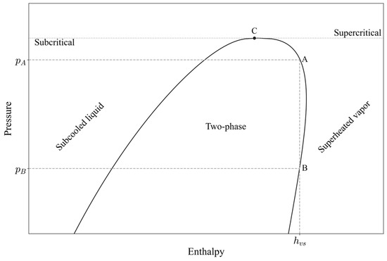
Figure 1. Log p–h diagram for propane illustrating the case of irreversibility between pressure and enthalpy predictions along the saturated vapor line.

Table 1 summarizes most of the studies that have addressed alternative approaches for determining thermophysical properties other than EOS, i.e., CoolProp or REFPROP. As shown in Table 1, the majority of these studies are validated either through a single property calculation [16,17,18,20], or component-level simulations [21], except for the SBTL method [19] and the implicit fitting method of Khoury [7], which are validated at the system level. Additionally, although the implicit fitting method is widely used, it presents notable challenges due to its complexity in identifying the correct physical solution. In contrast, the explicit method offers a straightforward and easily implemented approach.

Table 1. Overview of the methods used for thermophysical properties calculations as alternatives to EOS (i.e., CoolProp or REFPROP), including the refrigerants tested for each method and the computational speed.

	Method	Tested Refrigerants	Validation Through	Computational Speed
Cleland et al. [14,15]	Explicit	R12, R22, R114, R502, R717, R134a	System level (simple vapor compression cycle)	-
Ding et al. [16,17]	Implicit	R22, R407C	Single property calculations	140–1000×
Kunick et al. [18,22]	SBTL	CO2, water	Single property calculations	225×
Sieres et al. [20]	Hybrid	R407C, R1234yf + supplementary data for (R113, R125, R134a, R404A, R409A, R717, RC318)	Single property calculations	-
Aute & Radermacher [21]	Explicit	R32, R407C, R407F, R410A, R1234yf	Component level (heat exchangers)	10–646×
Li et al. [19,23]	SBTL	R1234f	System level (air conditioning system)	2–4×
Khoury et al. [7]	Implicit	Propylene, ethylene, methane	System level (cascade refrigeration cycle)	30×
This study	Explicit	Propane (R290)	System level (dynamic heat pump cycle)	117×

Accordingly, the objective of the present work is to first develop explicit thermodynamic formulations for calculating the thermophysical properties of propane, which have not been addressed in any of the previous studies shown in Table 1. Secondly, this work aims to validate these formulations through a system-level air-source dynamic heat pump under various operating conditions, thereby providing a level of analysis that most existing explicit studies, which focus on single components, do not offer. The proposed formulations are designed to be:

• Computationally efficient, requiring minimal computational time;
• Accurate, to minimize errors in system simulations and/or optimization;
• Explicit, to eliminate the need for any iterative procedures;
• Uniform structure, can be easily implemented or extended to other refrigerants;
• Reversible, ensuring consistent property evaluation from different explicit formulae wherever applicable.

2. Methodology

The formulations of the thermophysical properties are developed using an explicit method to enable accurate and computationally efficient calculations. Polynomial and power-law forms are implemented, with the objective of maintaining a consistent structure for all equations, so that the method can be easily programmed and adapted for multiple refrigerants. Subsequently, a dynamic heat pump model is developed to validate the explicit formulations at the system level, while accounting for variable operating conditions, e.g., heat demand and water temperature. The thermophysical properties are classified into two main categories: thermodynamic properties (e.g., pressure and enthalpy) and transport properties (e.g., viscosity and thermal conductivity). In addition, the properties can also be categorized according to the thermodynamic state. Section 2.1 presents the development of the explicit formulations with respect to the thermodynamic state, namely saturated, single-phase, or two-phase. Furthermore, Section 2.2 provides a detailed description of the dynamic heat pump model includes the main system components, i.e., the heat exchangers, compressor, and throttle valve. Finally, the characteristics of the computer/hardware and the solver used for the simulations of the dynamic model are presented in Section 2.3.

2.1. Explicit Formulations

Empirical correlations can be employed to determine the thermophysical properties using an explicit approach [20,21]. Equations (1) and (2) are used to describe the thermophysical output property (TOP) as a function of the input variables (IVs) in polynomial and power-law forms, respectively. TOP can refer to any thermodynamic or transport property, while the IVs always represent one or two thermodynamic properties, with pressure being an IV for all developed explicit formulations.

$$TO{P}_{poly}=\sum _{i=0}^n{a}_i I{V}_1^i+ \sum _{i=0}^n{b}_i I{V}_1^i \sum _{i=0}^n{c}_i I{V}_2^i +\sum _{i=0}^n{d}_i I{V}_2^i$$

(1)

$$TO{P}_{pow}=e_0\prod _{i=1}^k{IV}_i^{e_i}$$

(2)

Equation (1) represents the polynomial form of two input variables, where $a$, $b$, $c$, and $d$ are the coefficients that result from the regression model (Section 3.1) and the summation upper bound $n$ is the order of the polynomial function (e.g., second or third). On the other hand, Equation (2) is a power-law form, in which $e$ is the set of coefficients and power values and the multiplication upper bound $k$ is the number of independent IVs. While the polynomial model approximates the thermophysical output property as a higher-order function of the selected input variables, the power-law model captures nonlinear dependencies through exponent-based relationships. To accurately evaluate the developed thermodynamic formulations, the mean absolute relative deviation (MARD) of each TOP is calculated using Equation (3) and assessed in the following subsections, where $m$ represents the number of data points employed in the regression model, which will be generated using CoolProp [12].

$$MARD={\displaystyle \frac{1}{m}} \sum _{i=1}^m\left|{\displaystyle \frac{{TOP\left(i\right)}_{CoolProp}-TO{P\left(i\right)}_{Explicit}}{TO{P\left(i\right)}_{CoolProp}}}\right|$$

(3)

2.1.1. Saturated Properties

The saturated thermophysical properties have been evaluated for both the liquid and vapor states. The saturated data can fit a simple form of Equation (1), which depends on one IV, as shown in Equation (4), except for the pressure–temperature ($p$-$T$) relation that follows Antoine’s equation. All saturated properties are functions of a single input: pressure [Pa]. The polynomial order can range up to 8, chosen to balance the least-squares error and the irreversibility issue.

$$TO{P}_{poly}=\sum _{i=0}^n{a}_i I{V}^i$$

(4)

According to Cleland [14], in explicit formulations, one relation has to be reversible: the pressure–temperature calculations along the vapor-saturated line. Equation (5) represents the form of the Antoine equation [24] to calculate the saturated pressure ($p_s$) in Pa. Additionally, the same set of coefficients/parameters can be usually used to calculate the saturated temperature ($T_s)$ in K using Equation (6).

$$p_s=\mathit{exp}\left(e_0-{\displaystyle \frac{e_1}{T_s+e_2}}\right)$$

(5)

$$T_s={\displaystyle \frac{e_1}{e_0-ln\left(p_s\right)}}-e_2$$

(6)

The saturated properties (TOP) of Equation (4) are a function of a single IV (pressure), but this IV has to be normalized to its critical value before it is used in Equation (4), so the pressure has to be divided by the critical pressure of the refrigerant implemented ($p_c$). In contrast, both the IV and the TOP are normalized in Equations (5) and (6) to allow for a reversible $p$-$T$ relation. For instance, $p_s$ from Equation (5) must be multiplied by $p_c$ to obtain its absolute value in pascals (Pa).

2.1.2. Single-Phase Properties

This section presents both the superheated and subcooled thermophysical properties. Generally, all single-phase properties are functions of two IVs: $p$ and $h$, $T$, or $s$, based on the definition of the TOP. Equation (1) can be used to represent the polynomial form of the properties in the single-phase zones. The polynomial order for each property should be selected in order to minimize the least-squares error of the regression model, i.e., to maximize the accuracy of the predicted single-phase property. Additionally, one reversible relation has been introduced: the enthalpy-entropy ($h$-$s$) relation in the superheated zone. Equation (2) could predict the vapor enthalpy ($h_v$) in J/kg as a function of pressure [Pa] and entropy [J/kgK] in the power-law form as stated in Equation (7). In contrast, Equation (8) reverses the value of the entropy ($s_v$) as a function of pressure and enthalpy. As stated previously, to allow for a reversible $h$-$s$ relation, all the IVs and TOP in Equations (7) and (8) are normalized separately by their respective critical values.

$$h_v={ e}_0 p^{e_1} s^{e_2}$$

(7)

$$s_v={\left({\displaystyle \frac{h}{e_0 p^{e_1}}}\right)}^{({\displaystyle \frac{1}{e_2}})}$$

(8)

2.1.3. Two-Phase Properties

Most of the thermophysical two-phase properties can be calculated using Equation (10) based on the saturated properties and the vapor quality [25].

$$x={\displaystyle \frac{h -{ h}_{ls}}{h_{vs}-{ h}_{ls}}}$$

(9)

$$TO{P}_{TP}=\left(1-x\right) TO{P}_{ls}+x TO{P}_{vs}$$

(10)

The vapor quality, $x$, is calculated using Equation (9) as a function of the enthalpy in the two-phase zone ($h$) and the saturated liquid and vapor enthalpies, $h_{ls}$ and $h_{vs}$, respectively. Accordingly, by referencing the saturated liquid and vapor states from Section 2.1.1, Equation (10) can be applied to calculate the enthalpy [J/kg], entropy [J/kgK], and specific volume [m³/kg] in the two-phase zone as functions of $p$ and $x$. The density can be determined then as the reciprocal of the specific volume. In contrast, the two-phase partial derivatives are described by the general polynomial form given in Equation (1). Therefore, a general regression model is applied to these properties, in the same manner as for the other single-phase properties. The only difference is that the IVs in this case are $p$ and $x$.

2.2. Dynamic Heat Pump Model

A dynamic heat pump model is employed to examine the developed thermodynamic formulations for the various thermophysical properties. A basic heat pump system consists of two heat exchangers functioning as a condenser and an evaporator, a compressor, and a throttle valve.

2.2.1. Heat Exchangers

Modelling low-charge heat pumps makes the governing dynamics concentrate in the heat exchangers [26]. Therefore, the developed dynamic model is characterized by time-varying phase boundaries within the heat exchangers. Model assumptions are summarized in [26,27].

$${\displaystyle \frac{\mathsf{\partial }{\rho }_r}{\mathsf{\partial }t}}+{\displaystyle \frac{\mathsf{\partial }{\left(\rho v\right)}_r}{\mathsf{\partial }L}}=0$$

(11)

$${\displaystyle \frac{\mathsf{\partial }{\left(\rho u\right)}_r}{\mathsf{\partial }t}}+{\displaystyle \frac{\mathsf{\partial }{\left(\rho uv+pv\right)}_r}{\mathsf{\partial }L}}+{\displaystyle \frac{\mathsf{\partial }(\alpha \Delta {T)}_r}{\mathsf{\partial }L}}=0$$

(12)

$${\left(c_p\rho A\right)}_m{\displaystyle \frac{\mathsf{\partial }{T}_m}{\mathsf{\partial }t}}-{\displaystyle \frac{\mathsf{\partial }(\alpha \Delta {T)}_r}{\mathsf{\partial }L}}+{\displaystyle \frac{\mathsf{\partial }(\alpha \Delta {T)}_{sf}}{\mathsf{\partial }L}}=0$$

(13)

$${\left(c_p\rho A\right)}_{sf}{\displaystyle \frac{\mathsf{\partial }{T}_{sf}}{\mathsf{\partial }t}}-{\left(c_p\rho Av\right)}_{sf}{\displaystyle \frac{\mathsf{\partial }{T}_{sf}}{\mathsf{\partial }L}}-{\displaystyle \frac{\mathsf{\partial }(\alpha \Delta {T)}_{sf}}{\mathsf{\partial }L}}=0$$

(14)

The refrigerant mass balance, refrigerant energy balance, metal wall energy balance, and secondary fluid energy balance are represented in Equations (11)–(14), respectively, where the subscript $r$ refers to the refrigerant, $m$ to the metal wall, and $sf$ denotes the secondary fluid, either water or air. $\rho$ is density, $t$ is time, $v$ is velocity, $L$ is the length in the flow direction, $u$ is internal energy, $p$ is pressure, $\alpha$ is heat transfer coefficient, $c_p$ is the specific heat, $A$ is the cross-sectional area, and $\Delta T$ is the temperature difference between the refrigerant or the secondary fluid and the metal wall. The heat transfer coefficient, α, is determined using the references in Table 2, with experimental correlations that depend on the refrigerant phase/secondary fluid type, as well as the heat exchanger type.

Table 2. Correlations used for heat transfer coefficient calculations in the heat exchangers.

Phase	Condenser	Evaporator
SH	[28]	[29]
TP	[30]	[31]
SC	[32,33]	-
Water/air	[32,33]	[34]

To derive the governing equations, the mass and energy balances are integrated according to Leibniz’s rule. The condenser has been divided into three regions based on phase: superheating (SH), two-phase (TP), and subcooling (SC). In contrast, the evaporator has been divided into two regions: TP and SH. For instance, applying Leibniz’s rule to integrate Equation (12) with time-varying limits ($L_1$ and $L_2$) for a system with all three heat exchanger regions, as shown in Figure 2, yields the refrigerant energy balance for the two-phase region (Equation (15)). The governing equations for the other regions can be derived in the same manner as in [27]. As a result, the number of equations to be solved depends on the number of phase regions that exist in each heat exchanger at each time step.

$$\begin{array}{c}{A}_r \left[\begin{array}{c}\left(L_2-L_1\right)\left(h_{TP}{{\displaystyle \frac{\mathsf{\partial }{\mathsf{\rho }}_{\mathrm{r}}}{\mathsf{\partial }p}}}_{TP}+{\displaystyle \frac{1}{2}}\left(h_{TP}{\displaystyle \frac{\mathsf{\partial }{\mathsf{\rho }}_{\mathrm{r}}}{\mathsf{\partial }{h}_{TP}}}+{\mathsf{\rho }}_{\mathrm{T}\mathrm{P}}\right)\left({{\displaystyle \frac{\mathsf{\partial }\mathrm{h}}{\mathsf{\partial }p}}}_{vs}+{{\displaystyle \frac{\mathsf{\partial }\mathrm{h}}{\mathsf{\partial }p}}}_{ls}\right)-1\right)\\ +\left(L-L_2\right)h_{Ls}\left({{\displaystyle \frac{\mathsf{\partial }{\mathsf{\rho }}_{\mathrm{r}}}{\mathsf{\partial }p}}}_{SC}+{\displaystyle \frac{1}{2}}{\displaystyle \frac{\mathsf{\partial }{\mathsf{\rho }}_{\mathrm{r}}}{\mathsf{\partial }{\mathrm{h}}_{\mathrm{S}\mathrm{C}}}}{{\displaystyle \frac{\mathsf{\partial }\mathrm{h}}{\mathsf{\partial }p}}}_{ls}\right)-L_1{h}_{vs}\left({{\displaystyle \frac{\mathsf{\partial }{\mathsf{\rho }}_{\mathrm{r}}}{\mathsf{\partial }p}}}_{SC}+{\displaystyle \frac{1}{2}}{\displaystyle \frac{\mathsf{\partial }{\mathsf{\rho }}_{\mathrm{r}}}{\mathsf{\partial }{\mathrm{h}}_{\mathrm{S}\mathrm{H}}}}{{\displaystyle \frac{\mathsf{\partial }\mathrm{h}}{\mathsf{\partial }p}}}_{vs}\right)\end{array}\right]{\displaystyle \frac{dp}{dt}}\\ \hspace{1em}\hspace{1em}\hspace{1em}\hspace{1em}\hspace{1em}\hspace{1em}\hspace{1em}+A_r{h}_{ls}\left(L-L_2\right){\displaystyle \frac{1}{2}}{\displaystyle \frac{\mathsf{\partial }{\mathsf{\rho }}_{\mathrm{r}}}{\mathsf{\partial }{\mathrm{h}}_{SC}}}{\displaystyle \frac{d{h}_{out}}{dt}}-A_r\left({\mathsf{\rho }}_{\mathrm{T}\mathrm{P}}{h}_{TP}-{\mathsf{\rho }}_{\mathrm{S}\mathrm{H}}{h}_{vs}\right){\displaystyle \frac{d{L}_1}{dt}}\\ \hspace{1em}\hspace{1em}\hspace{1em}\hspace{1em}\hspace{1em}\hspace{1em}\hspace{1em}+A_r\left({\mathsf{\rho }}_{\mathrm{T}\mathrm{P}}{h}_{TP}-{\mathsf{\rho }}_{\mathrm{S}\mathrm{C}}{h}_{ls}\right){\displaystyle \frac{d{L}_2}{dt}}\\ \hspace{1em}\hspace{1em}\hspace{1em}\hspace{1em}\hspace{1em}\hspace{1em}\hspace{1em}={\dot{m}}_{r_{in}}{h}_{vs}-{\dot{m}}_{r_{out}}{h}_{ls}-{\dot{Q}}_r-{\displaystyle \frac{1}{2}}{A}_r{L_{1}h}_{vs}{\displaystyle \frac{\mathsf{\partial }{\mathsf{\rho }}_{\mathrm{r}}}{\mathsf{\partial }{h}_{SH}}}{\displaystyle \frac{d{h}_{in}}{dt}}\end{array}$$

(15)

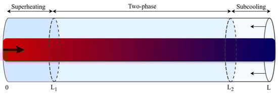
Figure 2. Schematic of the moving boundary model in the heat exchangers, solid arrows indicate the flow of refrigerant (bold) and secondary fluid (normal), while dashed lines represent the time-varying phase boundaries between the superheating, two-phase, and subcooling zones.

All thermophysical properties, including partial derivatives, in Equation (15) are calculated according to the explicit formulations developed in Section 2.1 using the saturated pressure and the associated mean enthalpy ($h$) of the respective refrigerant, assuming a linear enthalpy profile for each region (SH, TP, and SC).

2.2.2. Compressor

A variable-speed scroll compressor is used, featuring a swept volume of 46 cm³, and propane as the working fluid. The compressor is selected based on the technical data provided by Copeland for propane YHV models [35]. Furthermore, it was experimentally investigated by Ossorio et al. in their study [36]. Equation (16) calculates the compressor mass flow rate ${\dot{m}}_{CM}$, where $V_h$ is the stroke volume, $Z_{CM}$ is the compressor frequency,${ \rho }_{suc}$ is the refrigerant density at the suction point and ${\eta }_v$ is the volumetric efficiency.

$${\dot{m}}_{CM}=V_h Z_{CM}{ \rho }_{suc }{\eta }_v$$

(16)

2.2.3. Throttle Valve

A throttle valve with an orifice size of 2 mm is selected for a rated heating capacity of 10 kW using Danfoss Coolselector^®2 online software (version 5.4.9) for electronic expansion valves [37]. The mass flow rate of the throttle valve ${\dot{m}}_{TV}$ is calculated using Equation (17) as proposed by both Liu and Ma [38,39].

$${\dot{m}}_{TV}=C_{dis} A_{open} \sqrt{{ 2 \rho }_{i } | p_{i }-p_{o }|}$$

(17)

where $C_{dis}$ is the discharge coefficient calculated according to Li [40], $A_{open}$ is the valve opening area, and $i$& $o$ are subscripts for the inlet & the outlet of the valve, respectively.

2.3. Solver Setup

All regression and simulation models were performed on an HP EliteBook 845 G8 Notebook PC equipped with an AMD Ryzen 7 PRO 5850U processor (manufactured by TSMC, Hsinchu, Taiwan) running at 1.90 GHz and 16 GB installed RAM. The system operates on a 64-bit Windows 11 Enterprise environment (Version 22H2). The implementation was carried out in Python 3.11.5, using a numerical tolerance of 1 × 10⁻⁶ for regression and 1 × 10⁻⁵ for simulation

3. Results and Discussion

The explicit method proposed has been used to derive propane properties. The coefficients of the thermophysical properties of propane needed in the explicit formulations are determined by means of a regression model. Section 3.1 presents the coefficients of the explicit formulations according to the thermodynamic state, i.e., saturated, single-phase, or two-phase, along with a brief discussion of their accuracy in single-step calculations. Section 3.2 provides a general overview of single-property calculations using the explicit formulations within the different phase regions. Finally, Section 3.3 implements a system-level simulation of the dynamic heat pump model, where propane thermophysical properties are determined either by CoolProp (i.e., EOS) or by the explicit method developed in this work (Section 3.1). Detailed comparisons and simulation results, in terms of both accuracy and computational speed, are presented in the subsequent sections.

3.1. Propane Thermophysical Properties Formulation

A comprehensive set of empirical coefficients for propane has been developed to calculate its thermophysical properties using the explicit approach. The different data sets are generated from the open-source thermophysical property library CoolProp 6.4.1 [12]. CoolProp employs different methods for thermodynamic properties and transport properties, with the most accurate results obtained from the Helmholtz-energy-based formulations [13]. In addition, CoolProp is an open-source package compatible with most programming languages. Therefore, it is selected as the reference package for fitting and evaluating the explicit formulations.

The coefficients for both the polynomial and power-law models were obtained by fitting a regression to the CoolProp reference data using least-squares optimization. A convergence tolerance of 1 × 10⁻⁶ was employed to ensure high numerical accuracy. All regression models were executed in the Gekko optimization suite [41], utilizing steady-state estimation and the IPOPT solver. To normalize the input variables of the regression models, the critical properties of propane were calculated using CoolProp, resulting in a critical pressure of 4,251,200 Pa and a critical temperature of 369.89 K. Using the same approach, the corresponding enthalpy and entropy at the critical point were also evaluated based on these critical values.

3.1.1. Saturated Properties

The saturated properties of propane have been evaluated for both the liquid and vapor states. As the vapor compression cycles are neither operated under vacuum to eliminate air leakage into the system nor in the supercritical region, the data sets have been generated over an operating range from 1 to 42 bar. The saturated data of propane fit the simplified form of the polynomial function represented in Equation (4), with all properties functions of one IV, pressure.

The polynomial order ($n$) ranges from 6 to 8, which is selected to minimizes the least-squares error. Table 3 summarizes all the coefficients for the thermodynamic properties of propane. Along the saturated lines, all thermodynamic properties can be predicted with a deviation of less than 1%. While the MARD ranges from 0.04% to 0.99%, deviations exceeding 0.5% are commonly observed only along the saturated vapor line in calculations of density and its partial derivatives. It is worth noting that due to the flexibility provided by choosing the polynomial order, the saturated enthalpy (TOP) can be accurately computed from pressure (IV) using a 6th-order polynomial. This choice eliminated the need for two separate sets of equations, each covering a different pressure range as illustrated in Figure 1, resulting in predicted enthalpy values with a MARD of only 0.06%. All saturated thermodynamic functions in Table 3 are valid in a pressure range of 1–42 bar, except for the ${\displaystyle \frac{\mathsf{\partial }h}{\mathsf{\partial }p}}$, which is valid up to 35 bar. The explicit correlations were limited to a pressure of 35 bar to maintain low approximation error and an acceptable polynomial order, which represents a suitable operational range for the considered application. Extending the range to 42 bar is possible for most properties; however, this involves a trade-off between accuracy and computational efficiency.

Table 3. Summary of the coefficients of the thermophysical properties, including transport properties, along the saturated lines.

TOP	IV *	Coefficients										MARD [%]
		${\mathit{a}}_0$	${\mathit{a}}_1$	${\mathit{a}}_2$	${\mathit{a}}_3$	${\mathit{a}}_4$	${\mathit{a}}_5$	${\mathit{a}}_6$	${\mathit{a}}_7$	${\mathit{a}}_8$	${\mathit{a}}_9$
$h_{ls}$	p	6.277179 × 104	1.964730 × 106	−9.491604 × 106	3.305607 × 107	−6.907272 × 107	8.358675 × 107	−5.390112 × 107	1.433063 × 107			0.14
$h_{vs}$	p	5.085190 × 105	9.589499 × 105	−4.480009 × 106	1.326276 × 107	−2.291492 × 107	2.175289 × 107	−1.013718 × 107	1.630479 × 106			0.06
${\rho }_{ls}$	p	5.951765 × 102	−8.114157 × 102	2.463448 × 103	−5.084823 × 103	5.147672 × 103	−2.046156 × 103					0.16
${\rho }_{vs}$	p	−1.817414 × 100	1.780082 × 102	−1.132079 × 103	6.446548 × 103	−1.864401 × 104	2.897553 × 104	−2.284616 × 104	7.205610 × 103			0.86
${{\displaystyle \frac{\mathsf{\partial }\rho }{\mathsf{\partial }p}}}_{ls}$	p	6.668035 × 10−7	5.161540 × 10−5	−8.111962 × 10−4	7.147357 × 10−3	−3.493642 × 10−2	1.014348 × 10−1	−1.785439 × 10−1	1.869111 × 10−1	−1.070042 × 10−1	2.581443 × 10−2	0.73
${{\displaystyle \frac{\mathsf{\partial }\rho }{\mathsf{\partial }p}}}_{vs}$	p	2.552580 × 10−5	−6.716333 × 10−5	7.561922 × 10−4	−4.054468 × 10−3	1.308976 × 10−2	−2.527774 × 10−2	2.865627 × 10−2	−1.754043 × 10−2	4.472249 × 10−3		0.08
${{\displaystyle \frac{\mathsf{\partial }\rho }{\mathsf{\partial }h}}}_{ls}$	p	−5.133640 × 10−4	−1.638392 × 10−4	−3.123506 × 10−3	1.711386 × 10−2	−4.970691 × 10−2	7.296924 × 10−2	−5.287060 × 10−2	1.424223 × 10−2			0.12
${{\displaystyle \frac{\mathsf{\partial }\rho }{\mathsf{\partial }h}}}_{vs}$	p	1.291239 × 10−5	−1.091447 × 10−3	1.546427 × 10−2	−1.369754 × 10−1	6.642339 × 10−1	−1.910921 × 100	3.327506 × 100	−3.442333 × 100	1.945155 × 100	−4.624211 × 10−1	0.99
${{\displaystyle \frac{\mathsf{\partial }h}{\mathsf{\partial }p}}}_{ls}$	p **	1.096693 × 10−3	−8.514269 × 10−3	8.265211 × 10−2	−7.941606 × 10−1	4.353240 × 100	−1.474305 × 101	3.081097 × 101	−3.882611 × 101	2.703321 × 101	−8.029693 × 100	0.49
${{\displaystyle \frac{\mathsf{\partial }h}{\mathsf{\partial }p}}}_{vs}$	p **	−6.164527 × 10−2	4.254888 × 10−1	−4.181539 × 100	2.314938 × 101	−7.845433 × 101	1.626492 × 102	−2.016336 × 102	1.370797 × 102	−3.945517 × 101		0.09
$s_{ls}$	p	4.565605 × 102	8.138812 × 103	−4.223811 × 104	1.470626 × 105	−3.045237 × 105	3.638301 × 105	−2.312065 × 105	6.048254 × 104			0.14
$s_{vs}$	p	2.482619 × 103	−2.068351 × 103	1.466155 × 104	−5.791115 × 104	1.301558 × 105	−1.665122 × 105	1.125213 × 105	−3.121346 × 104			0.03
$c_{p_{ls }}$	p **	2.153762 × 103	4.438266 × 103	−1.838211 × 104	6.321710 × 104	−8.429590 × 104	−8.410648 × 104	4.384123 × 105	−5.361151 × 105	2.299859 × 105		0.02
$c_{p_{vs }}$	p **	1.333209 × 103	5.177076 × 103	−1.859664 × 104	4.058728 × 104	8.404440 × 104	−6.165551 × 105	1.319491 × 106	−1.281148 × 106	4.887251 × 105		0.05
${\mu }_{ls}$	p	2.339169 × 10−4	−2.023367 × 10−3	1.504931 × 10−2	−6.832342 × 10−2	1.869178 × 10−1	−3.103157 × 10−1	3.052950 × 10−1	−1.634295 × 10−1	3.662501 × 10−2		0.49
${\mu }_{vs}$	p	5.989728 × 10−6	1.670039 × 10−5	−1.700328 × 10−5	−2.901241 × 10−4	1.891598 × 10−3	−5.108098 × 10−3	7.138928 × 10−3	−5.062220 × 10−3	1.443422 × 10−3		0.17
${\sigma }_{ls}$	p	1.428795 × 10−1	−6.894171 × 10−1	5.543556 × 100	−2.935401 × 101	9.434132 × 101	−1.828424 × 102	2.082284 × 102	−1.280251 × 102	3.274391 × 101		0.30
${\sigma }_{vs}$	p	5.901932 × 10−3	3.037070 × 10−1	−4.525825 × 100	3.799685 × 101	−1.805905 × 102	5.121135 × 102	−8.821651 × 102	9.038784 × 102	−5.060191 × 102	1.191047 × 102	0.92

* Coefficients are valid for a pressure range of 1–42 bar, unless otherwise specified. A critical pressure of 4,251,200 Pa is used to normalize the IV, which is expressed in Pa. ** Valid for 1–35 bar.

The pressure–temperature calculations along the vapor-saturated line follow the reversible relation of Antoine (Equation (5)). Although the NIST Chemistry WebBook [24] provides three different sets of coefficients for the Antoine equation, each set covers a specific temperature range, which is limited based on the available data at that time [42,43,44]. To account for a wide temperature range (−30 to 90 °C), the CoolProp reference data are used with Equation (5) to generate new Antoine parameters, which are listed in Table 4 for the reversible relations. The new Antoine parameters can be used to calculate the saturated pressure or temperature with a MARD of only 0.04%.

Table 4. Summary of the coefficients for the reversible thermophysical properties calculated using Antoine’s equation and the power-law form.

TOP	IVs *	${\mathit{e}}_0$	${\mathit{e}}_1$	${\mathit{e}}_2$	MARD [%]
$T_s$	$p_s$	6.109454 × 100	6.128709 × 100	−3.125324 × 10−4	0.04
$h_v$	$p, s$**	1.018915 × 100	8.202058 × 10−2	1.295643 × 100	0.22

* Coefficients are valid for a pressure range of 1–42 bar. ** Specific entropy in the range of 2236–3206 kJ/kg·K.

3.1.2. Single-Phase Properties

Most of the superheated and subcooled thermodynamic properties of propane are developed using the explicit approach, following the general form of Equation (1). The polynomial order is selected to minimize the least-squares error of the regression model with values of 2 or 3 based on the identified property. Table 5 summarizes the different coefficients obtained from the regression models. The mean deviations range from 0.01% to 0.59%, with only one property exceeding this range: the partial derivative of density with respect to enthalpy. The coefficients for the single-phase properties presented in Table 5 are applicable within a pressure range of 1–42 bar. Additionally, a second independent IV is always required, either temperature (ranging from −20 to 90 °C for the superheated zone and 10 to 60 °C for the subcooled zone) or an equivalent enthalpy value. The use of two distinct temperature/enthalpy ranges is justified by the fact that, in most refrigeration applications, refrigerant subcooling is limited, as noted by Ding [16].

Table 5. Summary of the coefficients for thermodynamic properties of the single-phase (superheated or subcooled) and the two-phase zones.

TOP	IVs *	Coefficients								MARD [%]
		${\mathit{a}}_0$	${\mathit{a}}_1$	${\mathit{a}}_2$	${\mathit{a}}_3$	${\mathit{b}}_0$	${\mathit{b}}_1$	${\mathit{b}}_2$	${\mathit{b}}_3$
		${\mathit{c}}_0$	${\mathit{c}}_1$	${\mathit{c}}_2$	${\mathit{c}}_3$	${\mathit{d}}_0$	${\mathit{d}}_1$	${\mathit{d}}_2$	${\mathit{d}}_3$
$h_l$	p, T	1.129392 × 104	7.701423 × 104	8.983638 × 104		3.670759 × 103	−9.972746 × 102	−1.207874 × 103		0.30
		−4.254477 × 101	2.847762 × 102	−1.703285 × 102		1.129392 × 104	−1.072606 × 106	1.272940 × 106
$h_v$	p, T	1.553086 × 105	−4.695794 × 105	−1.554761 × 105		−3.072311 × 102	−4.229498 × 102	−4.507886 × 101		0.09
		1.131817 × 102	−1.199205 × 103	3.374640 × 101		1.553086 × 105	−8.905014 × 104	2.141645 × 105
${\rho }_l$	p, h	3.784637 × 101	6.386896 × 101	1.112858 × 102		−9.142976 × 100	1.062723 × 100	2.233408 × 100		0.17
		−5.953315 × 101	3.572162 × 101	−2.753395 × 101		3.784637 × 101	1.244215 × 102	−3.940168 × 102
${\rho }_v$	p, h	1.120135 × 100	5.557948 × 101	7.497828 × 100	−2.300015 × 101	−7.449341 × 10−1	1.845219 × 101	2.586909 × 101	4.383896 × 101	0.22
		7.338843 × 101	−1.627056 × 102	1.230116 × 102	−3.150931 × 101	1.120135 × 100	4.596546 × 100	−8.240646 × 100	2.774309 × 100
$T_l$	p, h	2.556397 × 100	−8.130716 × 100	−1.530595 × 101		1.925457 × 101	5.883220 × 10−1	1.202984 × 100		0.05
		9.202976 × 100	1.221585 × 101	−8.339775 × 100		2.556397 × 100	4.452390 × 101	7.893746 × 101
$T_v$	p, h	4.940026 × 101	1.674308 × 102	1.490256 × 101		−1.649456 × 101	3.763025 × 101	3.666424 × 100		0.01
		2.165388 × 101	−3.560540 × 101	1.267272 × 101		4.940026 × 101	4.775351 × 101	7.715888 × 101
${{\displaystyle \frac{\mathsf{\partial }\rho }{\mathsf{\partial }p}}}_l$	p, h	−8.764218 × 10−6	1.858684 × 10−5	−5.535698 × 10−6	−1.120303 × 10−7	4.617422 × 10−7	4.138042 × 10−5	−1.232813 × 10−5	−1.400531 × 10−7	0.16
		−1.477821 × 10−2	−2.908063 × 100	6.501049 × 100	−5.009068 × 100	−8.764218 × 10−6	1.266335 × 10−4	−2.759654 × 10−4	2.155234 × 10−4
${{\displaystyle \frac{\mathsf{\partial }\rho }{\mathsf{\partial }p}}}_v$	p, h	−8.976424 × 10−2	2.954839 × 10−5	6.374048 × 10−5		−4.399995 × 10−1	−2.316223 × 10−5	−8.452358 × 10−5		0.59
		−4.082777 × 10−1	3.775858 × 10−1	4.204950 × 10−1		-8.976424 × 10−2	1.659949 × 10−1	1.850692 × 10−1
${{\displaystyle \frac{\mathsf{\partial }\rho }{\mathsf{\partial }h}}}_l$	p, h	−7.613286 × 10−2	7.717079 × 10−4	7.631873 × 10−6		−3.932192 × 10−1	2.180793 × 10−3	8.638971 × 10−5		0.25
		−3.853270 × 10−1	8.999532 × 10−2	1.284674 × 10−1		−7.613286 × 10−2	3.669142 × 10−2	4.834510 × 10−2
${{\displaystyle \frac{\mathsf{\partial }\rho }{\mathsf{\partial }h}}}_v$	p, h	−1.573481 × 10−1	2.063333 × 10−2	7.214778 × 10−2	1.934503 × 10−1	−6.239372 × 10−1	5.795935 × 10−2	2.019784 × 10−1	5.409049 × 10−1	1.30
		−5.044212 × 10−1	3.296958 × 10−1	−2.488167 × 10−1	6.306116 × 10−2	−1.572911 × 10−1	2.055279 × 10−1	−1.551316 × 10−1	3.932572 × 10−2
${{\displaystyle \frac{\mathsf{\partial }\rho }{\mathsf{\partial }p}}}_{TP}$	p **, x	−4.514925 × 10−5	5.223494 × 10−5	1.536652 × 10−3	−1.682972 × 10−3	1.373035 × 10−6	−1.644559 × 10−7	−4.511200 × 10−6	5.055388 × 10−6	0.48
		9.612232 × 101	6.646908 × 102	−6.563252 × 102	2.298657 × 102	−4.518049 × 10−5	−9.685366 × 10−4	9.621914 × 10−4	−3.387376 × 10−4
	p ***, x	2.231093 × 10−5	1.217002 × 10−4	−1.308192 × 10−4	7.094978 × 10−5	−1.890104 × 10−4	7.179963 × 10−4	−9.272201 × 10−4	4.006302 × 10−4	0.29
		−5.063900 × 10−2	−1.649334 × 101	3.553504 × 101	−1.818629 × 101	2.231093 × 10−5	−1.064762 × 10−4	8.844992 × 10−5	−3.167679 × 10−5
${{\displaystyle \frac{\mathsf{\partial }\rho }{\mathsf{\partial }h}}}_{TP}$	p **, x	−8.653346 × 10−5	−3.410015 × 10−4	−6.280670 × 10−4	−6.042105 × 10−4	1.502221 × 10−6	6.835770 × 10−5	−8.312862 × 10−3	3.661317 × 10−3	1.39
		2.029297 × 100	−6.416609 × 100	6.660278 × 100	−2.407215 × 100	−8.653346 × 10−5	5.741837 × 10−4	−6.548470 × 10−4	2.556679 × 10−4
	p ***, x	−4.431150 × 10−4	−3.394996 × 10−3	8.028011 × 10−4	9.247058 × 10−4	3.261141 × 10−3	−1.343220 × 10−2	1.957269 × 10−2	−9.771804 × 10−3	1.10
		−2.802331 × 100	1.231034 × 101	−9.982051 × 100	2.324846 × 100	-4.431150 × 10−4	3.521560 × 10−3	−1.772630 × 10−3	2.437415 × 10−4

* Single-phase coefficients are valid for a pressure range of 1–42 bar and temperatures of −20 to 90 °C in the superheated zone and 10 to 60 °C in the subcooled zone, unless otherwise specified. Two-phase coefficients are valid for a vapor quality range of 0.5–1. A critical pressure of 4,251,200 Pa and a critical temperature of 369.89 K are used to normalize the IVs. ** Valid for 1–27 bar. *** Valid for 27–42 bar.

On the other hand, the $h$-$s$ relation in the superheated zone follows Equation (7) and can be reversed using Equation (8), with parameters summarized in Table 4 for reversible relations. The developed correlations show mean deviations of 0.22% and 0.17%, respectively, with a maximum absolute relative deviation of 1%. The $h$-$s$ relation follows the same validity range discussed above.

3.1.3. Two-Phase Properties

Equation (10) is used to determine most of the thermodynamic two-phase properties of propane (e.g., enthalpy, entropy, and density) based on the saturated properties and the vapor quality [26]. However, the partial derivatives do not follow the same formulation; therefore, a separate set of coefficients is developed for these properties using Equation (1). Table 5 summarizes the coefficients for the partial derivates, with minimum and maximum mean deviation of 0.29% and 1.39%, respectively. It is worth noting that the two-phase partial derivatives listed in Table 5 are divided into two regions by a pressure threshold of 27 bar, which corresponds to the maximum enthalpy within the two-phase zone. In both regions, the applicable vapor quality ranges from 0.5 to 1, which is suitable for dynamic model simulations that employ a linear enthalpy profile in the two-phase region [26,27], as specified in Section 2.2.1.

3.1.4. Transport Properties

This section presents the transport properties of propane, such as specific heat capacity ($c_p$) in J/kgK, dynamic viscosity ($\mu$) in kg/ms, and thermal conductivity ($\sigma$) in W/mK. The saturated transport properties can be calculated as a function of $p$ using Equation (4) and the coefficients summarized in Table 3, which are valid for a pressure range from 1 bar to 42 bar in the case of $\mu$ and $\sigma$, and to 35 bar in case of $c_p$. Both the specific heat capacity and thermal conductivity of the saturated liquid line showed lower mean deviations than those of the saturated vapor line. In contrast, the MARD of the dynamic viscosity is smaller for the saturated vapor line, with only 0.17%.

Single-phase and two-phase transport properties are represented using Equation (1) as a function of pressure ($p$) and enthalpy ($h$) or vapor quality ($x$), respectively. The resulting coefficients are summarized in Table 6. The two-phase transport properties of propane are presented using Equation (1) rather than Equation (10), as it provides higher accuracy. Further details are given in the Appendix A. The applicable pressure range for most transport properties extends from 1 bar to 42 bar, except for the two-phase specific heat and thermal conductivity, which are limited to a maximum pressure of 15 bar. This 15 bar limit was selected for two reasons: the application and the specified function employed. The former will be discussed later in Section 3.2, while the latter concerns the least-squares error associated with the shape of the polynomial function used (Equation (1)) and its highest polynomial order, which is set to 3. This is done to ensure a consistent structure across all equations, allowing the method to be easily programmed and adapted for multiple refrigerants. Both $h$ and $x$ serve as a second independent IV in this context, and they follow the same ranges previously defined for the single-phase and two-phase thermodynamic properties, respectively. The mean deviation of all liquid and vapor transport properties is below 0.14%, except for the vapor specific heat capacity, which reaches a maximum deviation of 0.52%. The two-phase thermal conductivity showed the smallest mean deviation of 0.32%, followed by viscosity at 0.92% and specific heat capacity at 0.97%.

Table 6. Summary of the coefficients for transport properties of the single-phase (liquid or vapor) and the two-phase zones.

TOP	IVs *	Coefficients								MARD [%]
		${\mathit{a}}_0$	${\mathit{a}}_1$	${\mathit{a}}_2$	${\mathit{a}}_3$	${\mathit{b}}_0$	${\mathit{b}}_1$	${\mathit{b}}_2$	${\mathit{b}}_3$
		${\mathit{c}}_0$	${\mathit{c}}_1$	${\mathit{c}}_2$	${\mathit{c}}_3$	${\mathit{d}}_0$	${\mathit{d}}_1$	${\mathit{d}}_2$	${\mathit{d}}_3$
$c_{p_l}$	p **, h	3.887493 × 102	9.308037 × 102	−1.541758 × 102		−1.310200 × 102	9.627313 × 101	−1.694776 × 101		0.14
		−2.084946 × 101	5.064505 × 101	−6.394510 × 101		3.887493 × 102	8.263334 × 102	3.908543 × 102
$c_{p_v}$	p **, h	7.870201 × 102	1.046585 × 103	3.565992 × 102	−1.106771 × 102	1.629281 × 101	−2.463849 × 102	1.315633 × 103	−4.363945 × 103	0.52
		−2.843074 × 103	6.939557 × 103	−5.652565 × 103	1.536302 × 103	7.870201 × 102	1.967108 × 101	−4.538841 × 102	4.562619 × 102
${\mu }_l$	p, h	−5.133854 × 10−5	−1.615936 × 10−4	1.391544 × 10−4		−1.840980 × 10−4	−5.809621 × 10−5	4.748284 × 10−5		0.10
		−1.972308 × 100	−3.827614 × 100	3.741860 × 100		−5.133854 × 10−5	−1.172262 × 10−3	9.471965 × 10−4
${\mu }_v$	p, h	−7.873145 × 10−6	2.732609 × 10−6	1.312679 × 10−5	1.299455 × 10−5	−4.851413 × 10−7	−1.180423 × 10−5	−9.974825 × 10−5	−1.143823 × 10−4	0.02
		−3.101727 × 100	7.351016 × 100	−5.660565 × 100	1.466484 × 100	−7.873145 × 10−6	3.896398 × 10−5	−2.120832 × 10−5	4.713206 × 10−6
${\sigma }_l$	p, h	7.266051 × 10−2	9.647177 × 10−3	−9.644094 × 10−4		−8.481371 × 10−3	4.578544 × 10−3	−6.999685 × 10−4		0.02
		−9.564155 × 10−1	−1.461914 × 100	2.742559 × 100		7.266048 × 10−2	−1.623706 × 10−1	7.341013 × 10−2
${\sigma }_v$	p, h	−5.244415 × 10−3	2.003390 × 10−2	−1.826475 × 10−3	3.181238 × 10−1	5.513272 × 10−3	−4.525813 × 10−2	3.468310 × 10−2	−1.213066 × 100	0.06
		−8.239147 × 100	2.033870 × 101	−1.627834 × 101	4.357878 × 100	−5.244415 × 10−3	5.984555 × 10−3	2.131177 × 10−2	−5.075550 × 10−3
$c_{p_{TP}}$	p ***, x	3.700939 × 103	5.616383 × 103	−1.416538 × 104	3.992688 × 104	1.742173 × 103	−1.495369 × 104	8.989452 × 104	−3.383184 × 105	0.97
		−6.157997 × 100	2.252606 × 101	−2.721375 × 101	1.099328 × 101	3.700939 × 103	−2.087525 × 104	2.394372 × 104	−9.353124 × 103
${\mu }_{TP}$	p, x	3.038418 × 10−6	1.419590 × 10−5	−4.895544 × 10−6	1.030746 × 10−5	−3.861583 × 10−6	4.156706 × 10−6	−5.342764 × 10−5	3.130126 × 10−5	0.92
		−4.087694 × 10−1	1.834401 × 100	−1.422877 × 100	4.351982 × 10−1	3.038418 × 10−6	9.218070 × 10−7	1.650756 × 10−6	−9.968602 × 10−7
${\sigma }_{TP}$	p ***, x	6.449879 × 10−3	6.882147 × 10−2	−1.605759 × 10−1	3.884211 × 10−1	2.392448 × 10−3	−1.840251 × 10−2	4.703344 × 10−2	−4.732724 × 10−1	0.32
		−3.212014 × 100	1.252229 × 101	−1.463863 × 101	5.792517 × 100	6.449879 × 10−3	−1.030520 × 10−2	1.054011 × 10−2	−3.760987 × 10−3

* Coefficients are valid for a pressure range of 1–42 bar, unless otherwise specified. ** Valid for 1–35 bar. *** Valid for 1–15 bar.

3.2. Single-Property Analysis

Figure 3 provides a graphical representation of the propane explicit thermodynamic formulations developed in this work across all zones (single-phase and two-phase) and the saturated lines. The distributions of enthalpy (Figure 3a) and temperature (Figure 3b) are determined using the explicit formulations of Section 3.1 and compared with the reference data from CoolProp, reporting the relative deviation between the two values. The enthalpy shows a common relative deviation of ±0.2% across all zones, except for two notable cases in which values reach ±7% under extreme subcooling or near the critical point. In contrast, the temperature shows a common relative deviation of only ±0.05%, with a maximum deviation of −1.8% near the critical point. Both of these cases fall outside the typical operating range of a standard vapor-compression cycle [16]. Consequently, it can be generally concluded that the developed explicit formulations behave consistently across all zones, with deviations that are negligible within this operating range. While the enthalpy and temperature heat maps in Figure 3 serve as illustrative examples of the relative deviations in thermophysical properties, most other properties behave similarly, with maximum deviations occurring only in the two notable cases discussed above.

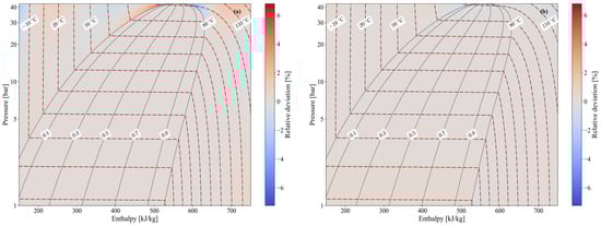
Figure 3. Heat maps of the relative deviation of enthalpy (a) and temperature (b) between the values predicted by the explicit formulations and the corresponding reference data from CoolProp over the investigated operating range.

In the same context, certain properties are applied only within specific ranges, such as the specific heat capacity and thermal conductivity in the two-phase region, as specified in Section 3.1.4. These properties are required solely for calculating the vaporization heat transfer coefficient [31]. Moreover, the evaporator typically operates at relatively low pressures. For instance, a pressure of 15 bar corresponds to a propane saturated temperature of 44 °C. Since the energy source, i.e., air, must be warmer than propane, the heat pump does not need to operate when the air temperature exceeds 44 °C. On the other hand, for cooling applications, the energy sink, i.e., water, should be much lower than 44 °C. Therefore, the 15 bar upper limit for both correlations is acceptable for the application presented in this work.

Figure 4 represents a validity map for the explicit formulations of propane. The operating range for the considered vapor compression cycle is indicated by the white (transparent) area, within which the formulations are globally valid over a pressure range of 1–35 bar for the developed moving-boundary HP model. The green lines represent a typical vapor compression cycle, for which the evaporation pressure is limited to an upper bound of 15 bar (≈44 °C), while the condensation pressure remains valid up to 35 bar (≈86 °C). This range covers typical residential heat pump applications but constitutes a limitation for other systems, such as high-temperature heat pumps. Within the white/transparent area, all explicit formulations exhibit negligible errors. Outside this range, the formulations are not applied: no extrapolation or clamping is performed, and the model is considered invalid beyond the defined operating range. It is worth noting that within the blue dashed region of Figure 4 (35–42 bar), certain thermophysical property correlations remain valid. However, because the moving boundary model relies on a fully consistent set of thermophysical property correlations, its overall range of applicability is governed by the most restrictive validity limit among them (35 bar). Consequently, the blue dashed region does not indicate deficiencies in the underlying physical assumptions or numerical scheme, but rather operating conditions that cannot be represented in a fully consistent manner within the presented moving-boundary modelling framework.

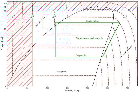
Figure 4. Validity map of the explicit formulations developed in this work. The white (transparent) region represents the intended operating range, with a typical vapor-compression cycle shown in green. The dashed-colored areas indicate regions where some explicit formulations remain valid but are not applicable to the specific moving boundary model considered (blue) or are outside the scope of this paper (red), such as extreme subcooling or near-critical operation.

3.3. Simulation Results

Two identical air-source heat pump models are developed, employing propane as the working refrigerant. The thermophysical properties of propane are determined either using CoolProp [12] or via the explicit formulations. The implementation of the simulations was carried out in Python 3.11.5, using a numerical tolerance of 1e-5 for both models. While the CoolProp model was solved using SciPy’s root function [45] and its modified Powell hybrid method (which combines the Gauss–Newton algorithm with gradient descent), the explicit model was simulated in the GEKKO package (version 1.3.0) [41] using the simultaneous moving horizon dynamic estimation and the IPOPT solver.

All thermophysical properties were evaluated using the CoolProp Python interface (PropsSI). Property calls were performed for scalar inputs inside the solver loop (i.e., no vectorized array evaluation was used), such that both the CoolProp model and the explicit model were subject to the same Python wrapper overhead. The CoolProp-based simulation was solved using a fixed time step of Δt = 10 ms in order to ensure numerical stability and convergence of the implicit formulation. The proposed explicit formulations were integrated using a fixed time step of Δt = 1 s, which was sufficient to accurately resolve the system dynamics in Gekko.

In the explicit simulations, the moving-boundary model is initialized in a three-zone configuration, with phase interfaces that move continuously via the boundaries ($L_1$ and $L_2$), as shown in Figure 2, This approach avoids sudden phase changes. As a result, there are no abrupt transitions between single- and two-phase formulations. The continuity of thermophysical properties and their derivatives across phase boundaries is verified through dedicated testing, resulting in smooth behavior similar to CoolProp. Consequently, no numerical chattering or convergence issues were observed, and the solver remained stable for all investigated operating conditions.

This air-source heat pump is evaluated using both model approaches to meet the heating demand illustrated in Figure 5a. The outdoor air temperature is set to a constant 3 °C, i.e., the average winter air temperature according to the National Belgian Weather Institute [46]. Figure 5 shows the outputs of the dynamic model for both approaches: CoolProp denotes the CoolProp-based simulation, and Explicit denotes the explicit method simulation. The Explicit results align with those obtained with CoolProp throughout the entire simulation period. The deviation in heating demand, shown in Figure 5a, is negligible (MARD = 0.005%) with a maximum difference of 0.009%. Figure 5b shows the condenser’s propane inlet temperature and water outlet temperature, with corresponding MARDs of only 0.12% and 0.01%, respectively. Lastly, the heat pump COP (Figure 5c) and propane mass flow rate (Figure 5d) show close agreement in the general trend and differ by only 1.12% and 0.88%, respectively. Overall, the minor deviation in COP and the negligible differences in both heating demand and outlet water temperature confirm that the explicit method provides an accurate representation of the system’s dynamic behaviour while maintaining excellent agreement with the CoolProp-based approach. A more detailed accuracy analysis is provided in Section 3.5.

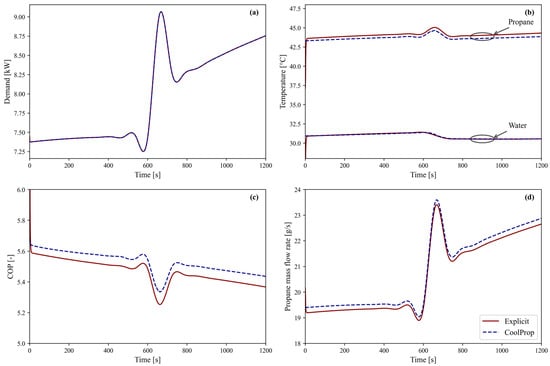
Figure 5. Overview of the dynamic behavior of the air-source heat pump model using both approaches, CoolProp and the Explicit method, over a 1200 s period: (a) heating demand, (b) propane inlet temperature and water outlet temperature at the condenser, (c) COP, and (d) propane mass flow rate.

3.4. Computational Speed

To quantify the computational performance of the system, three time categories were defined for the Explicit method and compared with the CoolProp approach. The first category is the CPU time required to calculate a single property, with examples for different phase states (e.g., liquid, two-phase). The second category is CPU time for initialization, which represents the time needed to set up the model. The third category is CPU time for the simulation, which reflects the total cumulative CPU time required to run the entire simulation. For single-property evaluations, the execution time was measured using the high-resolution function time.perf_counter_ns(). For model initialization and dynamic simulation with the Explicit method, the internal solver timing reported by GEKKO (SOLVETIME) was used. For consistency, the corresponding model initialization and simulation times when using CoolProp were measured using time.process_time(). Table 7 reports these three times, along with a speed-up factor noted in the last column. For the Explicit method, the CPU times for both single-property calculations (with density used as an example) and model initialization achieve a speed-up factor of several tens (e.g., 33 for liquid density and 32 for initialization), while the total simulation is accelerated by a factor of 117 compared to the CoolProp approach. This demonstrates the clear advantage of the Explicit method and its computational performance over the CoolProp-based approach.

Table 7. Comparison of CPU performance times between the CoolProp and Explicit simulations.

CPU Time		CoolProp	Explicit	Speed-Up Factor
Single-property [ms]	liquid	0.1896	0.0058	33
	Saturated liquid	0.1043	0.0037	28
	Two-phase	0.3181	0.0068	46
	Saturated vapor	0.1272	0.0054	24
	Vapor	0.252	0.0091	28
Initialization [s]		58.50	1.83	32
Simulation [s]		40,861	347.81	117

3.5. Accuracy

Table 8 summarizes the accuracy of the explicit thermodynamic properties for both the condenser and evaporator. Across all evaluated thermodynamic state variables, the explicit method demonstrates excellent agreement with the CoolProp reference calculations. For the condenser, the pressure and outlet enthalpy exhibit MARD values of 0.08% and 0.70%, respectively, while the corresponding maximum deviations remain below 1.06%. Propane temperature predictions in the SH, TP, and SC regions all remain within a MARD of 0.15% or lower. Tube-wall temperature estimates across all three corresponding zones differ by no more than 0.01% on average. Similarly, secondary fluid (water) inlet, core, and outlet temperatures show deviations below 0.01%. On the other hand, the evaporator deviations are even smaller: pressure and outlet enthalpy exhibit MARD values of 0.13% and 0.02%, respectively. Propane temperatures across SH and TP regions remain within 0.05% MARD, and the tube-wall temperatures maintain deviations as low as 0.01%. Air-side secondary fluid temperatures show the same level of accuracy, with MARD values of 0.01%. These results confirm that the explicit formulations reproduce the thermodynamic states with high precision throughout both heat exchangers. Combined with the significant computational performance reported in Section 3.4, the explicit method provides an attractive alternative to CoolProp/REFPROP for dynamic vapor-compression cycle simulations that require a balance between accuracy and computational speed. It should be noted that the proposed explicit formulations are obtained through independent regressions and are not derived from a single thermodynamic potential, and therefore are not explicitly constrained by Maxwell’s relations. This thermodynamic inconsistency is acknowledged as a limitation of the explicit method; however, it is considered acceptable for dynamic system modelling applications where computational efficiency is prioritized and only small errors are observed at both the system level (Section 3.3) and in the detailed accuracy analysis presented in this section.

Table 8. Accuracy analysis of the various thermodynamic state variables in the condenser and evaporator, reported in terms of Mean Absolute Relative Deviation (MARD) and maximum deviation between CoolProp-based and explicit simulations.

Thermodynamic State Variable			Condenser		Evaporator
			MARD [%]	Maximum Deviation [%]	MARD [%]	Maximum Deviation [%]
Pressure			0.08	0.23	0.13	0.32
Outlet enthalpy			0.70	1.06	0.02	0.05
Temperature	Propane	SH	0.12	0.15	0.05	0.08
		TP	0.01	0.03	0.01	0.04
		SC	0.15	0.21	-	-
	Tube-wall	1st zone	0.01	0.03	0.01	0.02
		2nd zone	0.01	0.04	0.01	0.03
		3rd zone	0.01	0.02	-	-
	Secondary fluid (Water/air)	Inlet	0.00	0.00	0.01	0.02
		Core	0.01	0.04	-	-
		Outlet	0.01	0.04	0.01	0.03

4. Conclusions

The explicit thermodynamic formulations offer a highly efficient alternative to conventional EOS-based calculations, such as those implemented in CoolProp/REFPROP. When applied to a dynamic air-source heat pump model, the explicit formulations achieves a speed-up factor of 117 while maintaining excellent accuracy with CoolProp. Deviations in heating demand are negligible, and the COP differs by about 1% only. Most thermodynamic state variables of the heat pump model show maximum relative deviations below 0.32%, with only the condenser outlet enthalpy remaining acceptable at 1.06%. These results clearly demonstrate the ability of the explicit method to capture the dynamic behaviour of vapor-compression systems with significant computational savings. Additionally, the explicit method represents a practical alternative to CoolProp/REFPROP for dynamic system simulations where both accuracy and computational efficiency are essential. The authors therefore recommend applying the explicit approach in future work to other low-GWP refrigerants, such as R600a and R454B, that are likely to become widely implemented.

References

- European Commission. Communication: An EU Strategy on Heating and Cooling; European Commission: Brussels, Belgium, 2016. [Google Scholar]
- Ritchie, H. Sector by Sector: Where Do Global Greenhouse Gas Emissions Come from? Our World Data, 18 September 2020. [Google Scholar]
- Shi, G.-H.; Aye, L.; Li, D.; Du, X.-J. Recent Advances in Direct Expansion Solar Assisted Heat Pump Systems: A Review. Renew. Sustain. Energy Rev. 2019, 109, 349–366. [Google Scholar] [CrossRef]
- Liansheng, L. Research Progress on Alternative Refrigerants and Their Development Trend. J. Refrig. 2011, 32, 53–58. [Google Scholar]
- European Commission. The Availability of Refrigerants for New Split Air Conditioning Systems That Can Replace Fluorinated Greenhouse Gases or Result in a Lower Climate Impact; European Commission: Brussels, Belgium, 2020. [Google Scholar]
- Höges, C.; Klingebiel, J.; Venzik, V.; Brach, J.; Roy, P.; Neumann, K.; Vering, C.; Müller, D. Low-GWP Refrigerants in Heat Pumps: An Experimental Investigation of the Influence of an Internal Heat Exchanger. Energy Convers. Manag. X 2024, 24, 100704. [Google Scholar] [CrossRef]
- Al Khoury, J.; Al Haddad, R.; Shakrina, G.; Malham, C.B.; Sayah, H.; Bouallou, C.; Nemer, M. A Fast Method for the Calculation of Refrigerant Thermodynamic Properties in a Refrigeration Cycle. Int. J. Refrig. 2024, 157, 98–108. [Google Scholar] [CrossRef]
- Zhao, D.; Ding, G.; Wu, Z. Extension of the Implicit Curve-Fitting Method for Fast Calculation of Thermodynamic Properties of Refrigerants in Supercritical Region. Int. J. Refrig. 2009, 32, 1615–1625. [Google Scholar] [CrossRef]
- Liu, J.; Wei, W.J.; Ding, G.L.; Zhang, C.; Fukaya, M.; Wang, K.; Inagaki, T. A General Steady State Mathematical Model for Fin-and-Tube Heat Exchanger Based on Graph Theory. Int. J. Refrig. 2004, 27, 965–973. [Google Scholar] [CrossRef]
- Span, R. Multiparameter Equations of State—An Accurate Source of Thermodynamic Property Data; Springer: Berlin/Heidelberg, Germany, 2000; ISBN 978-3-642-08671-7. [Google Scholar]
- Lemmon, E.W.; Huber, M.L.; McLinden, M.O. NIST Standard Reference Database 23: Reference Fluid Thermodynamic and Transport Properties-REFPROP; Version 9.1; NIST: Gaithersburg, MD, USA, 2013.
- Bell, I.H.; Wronski, J.; Quoilin, S.; Lemort, V. Pure and Pseudo-Pure Fluid Thermophysical Property Evaluation and the Open-Source Thermophysical Property Library Coolprop. Ind. Eng. Chem. Res. 2014, 53, 2498–2508. [Google Scholar] [CrossRef]
- Lemmon, E.W.; McLinden, M.O.; Wagner, W. Thermodynamic Properties of Propane. III. A Reference Equation of State for Temperatures from the Melting Line to 650 K and Pressures up to 1000 MPa. J. Chem. Eng. Data 2009, 54, 3141–3180. [Google Scholar] [CrossRef]
- Cleland, A.C. Computer Subroutines for Rapid Evaluation of Refrigerant Thermodynamic Properties. Int. J. Refrig. 1986, 9, 346–351. [Google Scholar] [CrossRef]
- Cleland, A.C. Polynomial Curve-Fits for Refrigerant Thermodynamic Properties: Extension to Include R134a. Int. J. Refrig. 1994, 17, 245–249. [Google Scholar] [CrossRef]
- Ding, G.; Wu, Z.; Liu, J.; Inagaki, T.; Wang, K.; Fukaya, M. An Implicit Curve-Fitting Method for Fast Calculation of Thermal Properties of Pure and Mixed Refrigerants. Int. J. Refrig. 2005, 28, 921–932. [Google Scholar] [CrossRef]
- Ding, G.L.; Wu, Z.; Wang, K.; Fukaya, M. Extension of the Applicable Range of the Implicit Curve-Fitting Method for Refrigerant Thermodynamic Properties to Critical Pressure. Int. J. Refrig. 2007, 30, 418–432. [Google Scholar] [CrossRef]
- Kunick, M.; Kretzschmar, H.-J.; Gampe, U. Fast Calculation of Thermodynamic Properties in Process Modeling Using Spline-Interpolation. In Proceedings of the 17th Symposium on Thermophysical Properties, Boulder, CO, USA, 21–26 June 2009. [Google Scholar]
- Li, L.; Gohl, J.; Batteh, J.; Greiner, C.; Wang, K. Fast Simulations of Air Conditioning Systems Using Spline-Based Table Look-up Method (SBTL) with Analytic Jacobians. In Proceedings of the American Modelica Conference, Boulder, CO, USA, 23–25 March 2020. [Google Scholar]
- Sieres, J.; Varas, F.; Martínez-Suárez, J.A. A Hybrid Formulation for Fast Explicit Calculation of Thermodynamic Properties of Refrigerants. Int. J. Refrig. 2012, 35, 1021–1034. [Google Scholar] [CrossRef]
- Aute, V.; Radermacher, R. Standardized Polynomials for Fast Evaluation of Refrigerant Thermophysical Properties. In Proceedings of the International Refrigeration and Air Conditioning Conference, West Lafayette, IN, USA, 14–17 July 2014. [Google Scholar]
- Kunick, M.; Kretzschmar, H.J. Guideline on the Fast Calculation of Steam and Water Properties with the Spline-Based Table Look-Up Method (SBTL); The International Association for the Properties of Water and Steam: Moscow, Russia, 2015. [Google Scholar]
- Li, L.; Gohl, J.; Batteh, J.; Greiner, C.; Wang, K. Fast Calculation of Refrigerant Properties in Vapor Compression Cycles Using Spline-Based Table Look-Up Method (SBTL). In Proceedings of the American Modelica Conference, Cambridge, MA, USA, 26 February 2019; pp. 77–84. [Google Scholar]
- U.S. Department of Commerce Propane, NIST Chemistry WebBook, SRD 69. Available online: https://webbook.nist.gov/cgi/cbook.cgi?ID=C74986&Mask=4F&Type=ANTOINE&Plot=on (accessed on 24 October 2025).
- Moran, M.J.; Shapiro, H.N.; Boettner, D.D.; Bailey, M.B. Fundamentals of Engineering Thermodynamics, 7th ed.; Wiley: Hoboken, NJ, USA, 2011; ISBN 9780470917688. [Google Scholar]
- Desideri, A.; Dechesne, B.; Wronski, J.; Van Den Broek, M.; Gusev, S.; Lemort, V.; Quoilin, S. Comparison of Moving Boundary and Finite-Volume Heat Exchanger Models in the Modelica Language. Energies 2016, 9, 339. [Google Scholar] [CrossRef]
- Bendapudi, S.; Braun, J.E.; Groll, E.A. A Comparison of Moving-Boundary and Finite-Volume Formulations for Transients in Centrifugal Chillers. Int. J. Refrig. 2008, 31, 1437–1452. [Google Scholar] [CrossRef]
- Longo, G.A. The Effect of Vapour Super-Heating on Hydrocarbon Refrigerant Condensation inside a Brazed Plate Heat Exchanger. Exp. Therm. Fluid. Sci. 2011, 35, 978–985. [Google Scholar] [CrossRef]
- Gnielinski, V. New Equations for Heat and Mass Transfer in Turbulent Pipe and Channel Flow. Int. Chem. Eng. 1976, 16, 359–367. [Google Scholar]
- Longo, G.A.; Righetti, G.; Zilio, C. A New Computational Procedure for Refrigerant Condensation inside Herringbone-Type Brazed Plate Heat Exchangers. Int. J. Heat. Mass. Transf. 2015, 82, 530–536. [Google Scholar] [CrossRef]
- Ghazali, M.A.H.; Mohd-Yunos, Y.; Pamitran, A.S.; Jong-Taek, O.; Mohd-Ghazali, N. Development of a New Correlation for Pre-Dry out Evaporative Heat Transfer Coefficient of R290 in a Microchannel. Int. J. Air Cond. Refrig. 2022, 30, 15. [Google Scholar] [CrossRef]
- Kim, M.B.; Park, C.Y. An Experimental Study on Single Phase Convection Heat Transfer and Pressure Drop in Two Brazed Plate Heat Exchangers with Different Chevron Shapes and Hydraulic Diameters. J. Mech. Sci. Technol. 2017, 31, 2559–2571. [Google Scholar] [CrossRef]
- Wanniarachchi, A.S.; Ratnam, U.V.; Tilton, B.E.; Dutta-Roy, K. Approximate Correlations for Chevron-Type Plate Heat Exchangers; American Society of Mechanical Engineers: New York, NY, USA, 1995. [Google Scholar]
- Kalantari, H.; Ghoreishi-Madiseh, S.A.; Kurnia, J.C.; Sasmito, A.P. An Analytical Correlation for Conjugate Heat Transfer in Fin and Tube Heat Exchangers. Int. J. Therm. Sci. 2021, 164, 106915. [Google Scholar] [CrossRef]
- Copeland Scroll Variable Speed Compressors. Available online: https://www.copeland.com/en-gb/shop/copeland-scroll-yhv1u-compressors (accessed on 3 October 2025).
- Ossorio, R.; Navarro-Peris, E. Study of Oil Circulation Rate in Variable Speed Scroll Compressor Working with Propane. Int. J. Refrig. 2021, 123, 63–71. [Google Scholar] [CrossRef]
- Danfoss Coolselector®2. Available online: https://www.danfoss.com/en/service-and-support/downloads/dcs/coolselector-2/#tab-overview (accessed on 3 October 2025).
- Liu, H.; Cai, J.; Kim, D. A Hierarchical Gray-Box Dynamic Modeling Methodology for Direct-Expansion Cooling Systems to Support Control Stability Analysis. Int. J. Refrig. 2022, 133, 191–200. [Google Scholar] [CrossRef]
- Ma, J.; Kim, D.; Braun, J.E.; Horton, W.T. Development and Validation of a Dynamic Modeling Framework for Air-Source Heat Pumps under Cycling of Frosting and Reverse-Cycle Defrosting. Energy 2023, 272, 127030. [Google Scholar] [CrossRef]
- Li, W. Simplified Modeling Analysis of Mass Flow Characteristics in Electronic Expansion Valve. Appl. Therm. Eng. 2013, 53, 8–12. [Google Scholar] [CrossRef]
- Beal, L.D.R.; Hill, D.C.; Martin, R.A.; Hedengren, J.D. GEKKO Optimization Suite. Processes 2018, 6, 106. [Google Scholar] [CrossRef]
- Kemp, J.D.; Egan, C.J. Hindered Rotation of the Methyl Groups in Propane. The Heat Capacity, Vapor Pressure, Heats of Fusion and Vaporization of Propane. Entropy and Density of the Gas. J. Am. Chem. Soc. 1938, 60, 1521–1525. [Google Scholar] [CrossRef]
- Rips, S.M. On a Feasible Level of Filling in of Reservoires by Liquid Hydrocarbons. Khim. Prom. 1963, 8, 610–613. [Google Scholar]
- Helgeson, N.L.; Sage, B.H. Latent Heat of Vaporization of Propane. J. Chem. Eng. Data 1967, 12, 47–49. [Google Scholar] [CrossRef]
- Virtanen, P.; Gommers, R.; Oliphant, T.E.; Haberland, M.; Reddy, T.; Cournapeau, D.; Burovski, E.; Peterson, P.; Weckesser, W.; Bright, J.; et al. SciPy 1.0: Fundamental Algorithms for Scientific Computing in Python. Nat. Methods 2020, 17, 261–272. [Google Scholar] [CrossRef]
- KMI. Klimaatstatistieken van de Belgische Gemeenten. Available online: https://www.meteo.be/en/belgium (accessed on 8 October 2025).
Disclaimer/Publisher’s Note: The statements, opinions and data contained in all publications are solely those of the individual author(s) and contributor(s) and not of MDPI and/or the editor(s). MDPI and/or the editor(s) disclaim responsibility for any injury to people or property resulting from any ideas, methods, instructions or products referred to in the content. |
© 2026 by the authors. Licensee MDPI, Basel, Switzerland. This article is an open access article distributed under the terms and conditions of the Creative Commons Attribution (CC BY) license.