Abstract
Lighter-than-air parakites deployed at sea in the close proximity of wind turbines may offer the possibility of mitigating wake losses encountered in large offshore wind farms. Such devices, having an order of magnitude similar to wind turbine rotors, can divert the stronger winds available at high altitudes to the lower level within the atmospheric boundary layer to enhance the wind flow between turbines. Mooring the parakites directly to the offshore wind turbine support structures would avoid the need for additional offshore structures. This paper investigates a novel and simple approach for mooring a parakite to an offshore wind turbine. The proposed approach exploits the lift forces of the inflatable parakite to reduce the tower bending moment at the base of the turbine induced by the rotor thrust. An iterative numerical model coupling the parakite loads to a catenary cable piecewise model is developed in Python 3.12.7 to quantify the bending moment reduction and shear load variations at the wind turbine tower base induced by the different kite geometries, windspeeds, and mooring cable lengths. The numerical model revealed that the proposed approach for mooring parakites can substantially reduce the tower bending loads experienced during rotor operation without considerably increasing the shearing forces. It was estimated that the tower bending moment decreased by 7.7% at the rated wind speed, where the rotor thrust is at its maximum, while the corresponding shear force increased by 0.6%. At higher wind speeds, where the magnitude of the rotor thrust decreases, the percentage reduction in bending moment gradually increases to 51.7% at a wind speed of 24 m/s, with the corresponding shear force increasing by only around 4.6%. Furthermore, while upscaling the parakite augments the tower bending moment reduction, changes in cable length had little effect on bending moment reduction and shear increase.
1. Introduction
Wind energy is projected to supply around 20% of the world’s energy demand by 2030 [1,2]. Recent studies highlight that wind energy is among the most cost-effective renewable energy resources (RES), with technology costs declining significantly over the past two decades [3,4].
Although offshore wind turbines are more expensive to deploy than their onshore counterparts, offshore installations offer several advantages, including higher wind speeds, lower wind shear, and reduced turbulence [3,5,6]. In addition, development constraints such as limited land availability, noise restrictions, and visual impacts are less pronounced at sea [7].
In 2021, global wind power generation reached a total installed capacity of approximately 837 GW, with Europe accounting for 236 GW of this figure. Of the total wind power generated, approximately 93% originated from onshore wind farms, while only 7% was contributed by offshore installations [7]. Notably, onshore wind capacity additions experienced a decline of 31% during that year. In contrast, offshore wind power capacity experienced a significant surge, increasing by more than threefold over the same period [8].
The most commonly deployed offshore wind turbine (OWT) foundations are monopiles, typically installed in water depths of up to 40 m [9]. Monopile foundations account for approximately 81% of all installed OWT. In recent years, advancements in foundation technologies have enabled the installation of fixed-bottom turbines in deeper waters, reaching depths of around 50 m [10]. Deploying wind turbines in deeper offshore locations offers notable advantages, including reduced influence from land-induced wind shear, thereby enhancing wind resource quality and energy yield [7].
Wake interactions are one of the key challenges for large offshore wind farms [11,12]. When wind passes through the rotor of a turbine, momentum is extracted and turbulence is generated, creating a wake that propagates downstream. Turbines located within this wake experience reduced wind speed and increased turbulence, decreasing power production and augmenting fatigue loads. Several studies have quantified the severity of this effect with typical wake losses estimated to range between 10% and 25% of annual yield for offshore wind farms, depending on turbine spacing, atmospheric conditions, and wind farm size [13,14]. Through numerous studies, it is suggested that the downstream wind turbine should be spaced no less than 7 to 12 rotor diameters downstream [13].
To mitigate wake losses and reduce the spacing between one turbine and the downstream wind turbine, this study introduces a novel system of an inflatable parafoil kite (parakite) moored to the wind turbine tower base through a horizontal strut. Inflating of the Parakite with the lighter-than-air gas enables it to maintain the required altitude even during periods of calm winds. By adjusting the angle of attack, the parakite generates downwash, which accelerates the airflow through the downwind turbines. In addition, the strong tip vortices are formed similar to those observed in aircraft flight-promote mixing between the undisturbed high-altitude wind and the slower-moving air in the turbine wake, thereby re-energising the flow [15,16].
One of the key challenges faced by fixed-based OWTs is the bending moment at the base of the tower, primarily induced by wind loads acting on the turbine blades. He et al. [17] found that the force generated by wind loads on the blades account for only about 5% of the total horizontal load when compared to wave-induced forces. Nevertheless, despite its relatively small magnitude, the wind load at the rotor has a disproportionately large impact on the structural behaviour due to the large tower height. It can contribute up to 50% of the horizontal displacement at the top of the monopile and significantly influence the maximum bending moment within the foundation. This highlights that, although wind loading appears minor relative to wave loading, it plays a critical role in the structural response and must be carefully considered in design [17].
The transfer of structural loads from the rotor hub to the foundation represents one of the principal engineering challenges in OWTs. The transition piece, positioned between the foundation structure and the turbine tower base, serves a critical function in transmitting aerodynamic and structural forces from the rotor assembly to the seabed. Consequently, transition pieces must be rigorously engineered to ensure reliable load transfer while mitigating the risk of structural failure. In practice, their design is frequently project-specific, tailored to site conditions and loading scenarios [18,19]. Implementation of the proposed system reduces the magnitude of forces acting on the transition piece, thereby enabling material optimisation and reducing both fabrication and engineering costs. D. Boonman et. al. [15] investigated a concept similar to that presented in this study for wake loss mitigation. However, their work assumed that the kite was moored to an independent offshore platform than to a wind turbine foundation.
This paper introduces a simple concept in which the parakite serves a dual function: mitigating wake losses while simultaneously reducing the bending moment at the tower base. The proposed novel system is presented in detail in Section 2. The paper aims to quantify the reduction in tower bending moments at a wind turbine foundation. An assessment of the potential energy gains in a wind farm setting through the proposed concept is beyond the scope of the present work. Section 3 outlines the workflow of the in-house-developed Python code and describes the implementation of the previously introduced equations. Assumptions, modelling conditions, and potential numerical discretisation errors are addressed in Section 4. Section 5 provides an in-depth analysis of the parakite’s behaviour and its mooring cable dynamics, while Section 6 summarises the key findings and suggests directions for future work.
2. Theory
The proposed system is shown in Figure 1. A horizontal strut is attached to the tower of the rigid monopile OWT and a mooring line extends from it to the parakite filled with a lighter-than-air gas. The parakite is designed such that its buoyancy is able to support its own weight and the weight of the cable, even at stagnant air when no wind, and hence no lift, is present. Any forces generated by the kite affect the moments acting on the base of the OWT. The following subsections will initially discuss the condition when no wind is blowing, followed by a discussion for the case in which both the OWT and the parakite are operating in a wind stream. When wind is considered, it is assumed to have a fixed flow velocity. The effects of ambient turbulence, as well as the aerodynamic influence of the wind turbine rotor and tower on the kite and tether, are neglected in this study. Consequently, the numerical model is formulated to determine the equilibrium position of the parakite in the atmosphere under undisturbed wind conditions, as if no wind turbine were present.
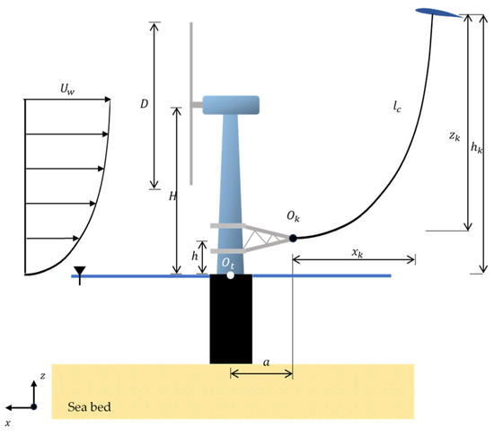
Figure 1.
The proposed system of an offshore wind turbine monopile with a moored parakite, where Uw is the free stream wind velocity, and D and H are the rotor diameter and hub height, respectively. a is the length of the horizontal strut from Ot, and h is the height of the horizontal strut from Ot. xk and yk are the coordinates of the parakite with respect to Ok. Both Ot and Ok are the origin of the turbine and kite, respectively.
2.1. Conditions of No Wind
Initially, it is assumed that no wind is present, so the lighter-than-air gas is only retained airborne due to the buoyancy force from the lifting gas. The inelastic cable secures the parakite at to the horizontal strut of length and at a height from the datum which is at sea level. The horizontal strut is assumed to be connected to the wind turbine tower via two collar bearings shown in Figure 1, which enable passive self-alignment of the parakite with varying wind directions. Securing the parakite to the horizontal strut takes place through a cable of length having a mass per unit length , while the total weight () is found using Equation (1). The parakite is filled with a gas that has a density much less than that of air, causing a lifting (buoyancy) force . The lifting force is due to the displaced parakite volume, , using Archimedes’ law and represented by Equation (2).
Helium was selected as the lifting gas in this study, as its lower density compared to air allows it to displace atmospheric air and generate buoyancy. The density of helium and air are obtained through CoolProp which is a Python library [20]. For an ambient temperature of 293 K, a density for helium () and air () of 0.164 kg·m−3 and 1.2 kg·m−3 are obtained, respectively. These densities were assumed to be constant when estimating the net buoyancy load and overall kite weight. The air temperature was treated as constant because its change within the 200 m layer is only about 2 K, which is sufficiently small enough to be considered negligible for the purposes of this study [21]. Consequently, the respective gas weight () is calculated using Equation (3), where is the internal volume of the parakite filled by helium. The kites’ skin () is calculated using Equation (4), where is the total surface area of the parakite and is the kite material in grams per square metre. The resulting lifting force at the initial stage is calculated using Equation (5). If the resultant force is greater than zero, the kite is capable of being airborne and supporting the weight of the cable. All the above-mentioned forces act when the parakite is not subjected to a wind force and are depicted in Figure 2. These are all assumed to act at the quarter position.
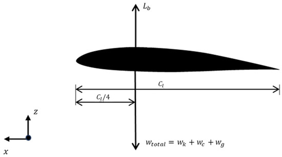
Figure 2.
Forces acting on the parakite section while subjected to no wind and having a buoyancy force Lb, weight of parakite skin wk, weight of cable wc, and weight of gas wg.
The surface area of the parakite is calculated by symmetrically dividing it into a series of sections along the parakite span (y-axis), each with a defined increment thickness, . At each of these sections, the cross-sectional aerofoil is further subdivided into smaller segments to calculate its circumferential length, denoted as . The total surface area of the kite, accounting for both upper and lower surfaces, is given by Equation (6).
Similarly, the volume of the parakite is computed by summing the cross-sectional areas along the y-direction (span-wise) and multiplying by the segment thickness. The cross-sectional area of the aerofoil () is determined using the shoelace formula, as shown in Equation (7). This formula calculates the area enclosed by a closed polygon based on its coordinates. Finally, the total volume of the parakite is determined by integrating these cross-sectional areas along its span, as shown in Equation (8), and accounting for symmetry by multiplying by 2.
2.2. Subjected to a Wind Force
When the parakite is subjected to a wind force, the inelastic mooring cable is expected to exhibit a profile similar to that of Figure 1. Throughout this study, it is assumed that the parakite is equipped with an automatic control system that positions it at a fixed optimal angle of attack (AOA), α. The parakite is assumed to operate at an angle of attack close to that corresponding to the maximum lift-to-drag ratio (), thereby ensuring optimal aerodynamic performance and stable, attached flow conditions for this preliminary analysis. Modelling this control system was beyond the scope of this study. As an initial boundary condition, the height of the parakite is initially assumed at half the rotor hub height (z). This height is then adjusted during the execution of iterative routine until the Python code establishes the equilibrium height for the static condition. The wind velocity at the prescribed height is computed using Equation (9). In Equation (9), and are the reference wind speed and the reference height, respectively. Moreover, is the height of the parakite with reference to the sea level while is the wind shear exponent.
The aerodynamic lift and drag induced by the parakite as a result of the wind force are calculated according to Equations (10) and (11), respectively, where for both equations, is the planform area, the 2-dimensional area of the curved parakite surface in the x-y plane. The density of air, , is technically dependent on the kite’s altitude, although it is being maintained constant in this study, equal to 1.2 kgm−3 due to small altitude (<200 m). Both coefficients of lift () and drag () are obtained through the Athena Vortex Lattice (AVL) code [22,23].
The AVL software V2.5 was developed by Mark Drela at the Massachusetts Institute of Technology (MIT). It extends the classical Vortex Lattice Method (VLM) to simulate the aerodynamic behaviour of lifting surfaces. The AVL code is capable of computing the lift distribution and induced drag for a given wing configuration by modelling vortices using a horseshoe vortex distribution along both the span and chord. The software is grounded in four fundamental aerodynamic principles: (1) the Biot–Savart Law, (2) the Kutta–Joukowski Theorem, (3) Helmholtz’s Vortex Theorems, and (4) Prandtl’s Lifting-Line Theory [22,23].
Since AVL models the pressure and induced drag components only from an AoA of −10° to 10°, a correction had to be applied to the drag predictions to account for viscous drag over the upper and lower surfaces of the parakite. In this correction, the parakite was approximated to be a flat plate aligned with the flow. The parakite was bisected into a number of flat plates through the span-wise direction. The coefficient of drag over a flat plate element was calculated using the Prandtl approximation [24], represented by Equation (12). In Equation (12), is based on the reference length equal to the chord length at that segment. Moreover, Equation (13) was utilised to calculate the drag over the corresponding flat plate. Finally, Equation (14) was utilised to summate the drag over all the flat plate elements making up the entire parakite curved surface.
Finally, the resultant forces acting on the parakite in the and directions are calculated through Equations (15) and (16), respectively. All the discussed resultant forces are shown in Figure 3 and are assumed to act at the quarter chord location.
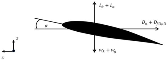
Figure 3.
Forces acting on the parakite while subjected to a wind force and inclined at an angle of attack α, having a buoyancy force Lb, aerodynamic force La, aerodynamic drag Da, drag induced by flat plate assumption Dfltplt, weight of parakite skin wk and weight of gas wg.
The cable is discretised into a number of nodes and elements to determine the resultant force acting at . The profile is followed by the cable when under the action of its own weight and force applied by the parakite at its upper end. Figure 4a depicts the discretisation of the cable into a number of straight-line elements from the 1st to the last Nth node. This approach is utilised throughout this study. This study assumes that the cable is homogeneously manufactured; thus, the weight of all elements are thought of as equal and acting at the midpoint of each element.
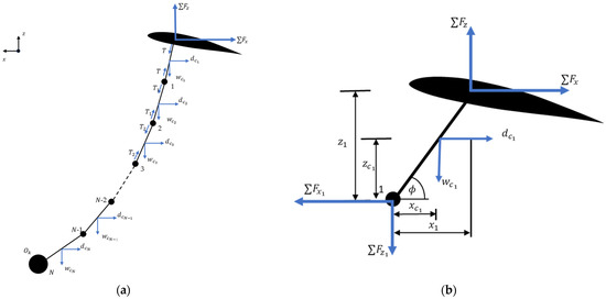
Figure 4.
(a) Cable nodal discretisation of the parakite to the wind turbine till node N and (b) first cable element discretisation (element 1) between the parakite and first node, defining all the forces acting in the x and z directions.
The position of the cable is determined by calculating the sum of moments at each element as a result of the and forces from the previous nodes along with the weight of the cable and its induced drag. Since the system is in a static position, the sum of moments at the node must equate to zero in order to satisfy equilibrium, in line with Equation (17). Moreover, Equation (17) assumes that the cable exerts constant drag. Figure 4b represents the top-most element of the cable while indicating all the forces acting upon it.
The following explains the notation of Equation (17); is the horizontal distance between the node and the kite, is the weight of the cable for the respective cable element, is the horizontal position of the mid-length of the cable, drag force induced over the cable, is the vertical position of the mid-length of the cable, and is the vertical distance between the node and the kite.
The cable horizontal drag is further calculated using Equation (18), with the area of each element assumed to be the area projected on a vertical plane. For Equation (18),
is the air density at the cable element height, is the cable diameter, is the wind speed at the element height, and is the cable coefficient of drag. In this study, is assumed to be equal to 1.2, corresponding to the drag coefficient of a cylinder normal to the flow for Reynolds number in the range – [25,26].
The weight of the cable at each element could be calculated through Equation (19). Moreover, the resultant forces acting at the subsequent node, node 1 of Figure 4b, in the x and z direction, are calculated through Equations (20) and (21), respectively.
The distance , , and of Equation (17) and Figure 4b could be solely expressed in terms of the cable length and the angle at which the element is positioned (), as presented by Equations (22)–(25). Substituting the mentioned equations into Equation (17), Equation (26) is obtained. Equation (26) could be further solved for as indicated by Equation (27). Substituting for and into Equations (24) and (25), the position of the previous node could be defined.
Repeating the procedure of Equations (17)–(27), for the length of the cable, its profile and the parakite’s position could be determined. This is achieved by summating the and values for each node, resulting in the and of Figure 1. Calculating the new parakite height, , through Equation (28) and then substituted into Equation (9), yields the wind speed at the new height. This procedure is carried out to refine the previous results as a result of the initial assumption, where it is initially assumed that the parakite height is at half-rotor-hub height.
The procedure from Equations (9)–(28) is repeated until the percentage difference in parakite height between successive calculations () is less than 0.5%. Equation (29) is utilised to ensure that the obtained distance will yield a zero-moment force at . Here, is the summation of induced moments by the weight of the cable and drag at each element with respect to . The forces in the x and z directions at the last node correspond to the forces exerted on the horizontal strut attached to the wind turbine structure, consequently resulting in moments acting at the base of the wind turbine, , as discussed in the following section.
2.3. Moments at the Base of the Wind Turbine
The forces acting on the wind turbine are shown in Figure 5, where the thrust () acting at the OWT rotor during operation in the presence of the wind induces a bending moment at the tower base. Throughout this study, it is assumed that the contribution of the tower drag to this moment is negligible.
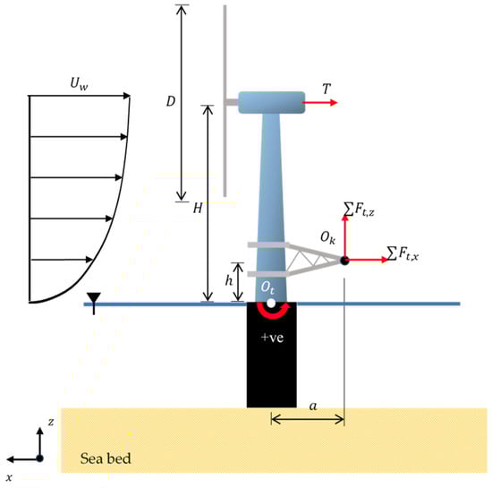
Figure 5.
Forces acting on the floating offshore wind turbine where T is the thrust generated by the wind turbine, with ∑Ft,z and ∑Ft,x resultant force due to the wind loads by the Parakite.
Equation (30) is used to calculate the total moment () acting at as a result of the horizontal and vertical forces induced both by the cable and parakite, and , respectively. Moreover, the thrust generated by the OWT is calculated using Equation (31), where it is dependent on the coefficient of thrust, the wind speed and air density at rotor hub height. The coefficient of thrust was derived from the thrust data presented by J. Jonkman et al. [27] for the National Renewable Energy Laboratory (NREL) 5-MW reference rotor. These data are reproduced in Figure 6 and were used to obtain the thrust coefficient of thrust, which was subsequently used in Equation (31). Finally, Equation (32) is utilised to calculate the percentage decrease in the bending moments at the tower base due to cable load induced by the parakite. The bending moment at the tower base, due to the weight of the horizontal strut, was ignored, as this was found to be only ≈2% of the maximum value induced by the rotor thrust.
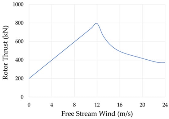
Figure 6.
Rotor thrust (kN) against free stream wind (m/s) for NREL 5 MW Rotor obtained from [27].
Moreover, the combined effect of the parakite and turbine thrust induces a force in the x-direction, which in turn influences the shear on the tower. The percentage increase in tower shear resulting from the drag forces acting on the parakite and its cable is calculated using Equation (33).
3. Numerical Model
This section describes how the mathematical equations of Section 2 were implemented into a numerical solution solved through an iterative process until the parakite achieves static equilibrium conditions. This was carried out using an in-house-built Python code, composed of 8 scripts which compute the forces at each node and the respective position. It also estimates the percentage bending moment decrease and percentage shear increase.
A high-level flow chart of the iterative routine implemented in the parakite Python code is presented in Figure 7. At the start of the simulation, user-defined input data is prescribed. The provided geometrical parameters are used to compute various parakite characteristics, including the internal volume, skin surface area, and skin weight. With the internal volume known, both the gas weight and the corresponding buoyant lifting force are calculated. Additionally, the cable weight is determined using its specified density and diameter. These values are then used to compute the resultant lifting force, . A conditional statement (if condition) is implemented to verify that the is large enough to provide a positive lifting force. If this is not the case, the code displays a message and terminates the computation.
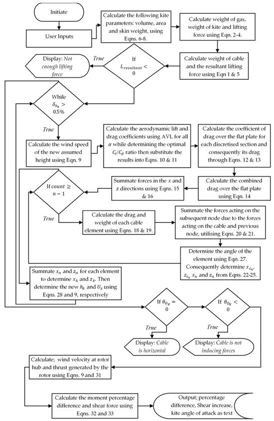
Figure 7.
Main execution flow chart of in-house-developed Python code.
If is greater than zero, the code proceeds to compute the lift coefficients for all angles of attack of the parakite. The angle of attack () is then determined based on the maximum ratio of to obtained from the AVL results. Using this , the lift and drag forces acting on the parakite are calculated. Since the AVL does not account for viscous drag, as mentioned in Section 2.2, the code compensates by estimating this drag over a flat plate. Finally, the total forces acting on the parakite in the x and z directions are determined by combining all components.
The code executes an if loop that uses a variable, count, representing the element number composing the cable. For each element, the Python code calculates the drag force acting on the element and its corresponding weight, applied through its centre. It then computes the x and z components of the forces acting on the subsequent node, based on contributions from both the cable element and the preceding node. Within the same loop, the code determines the cable element’s angle for that section and subsequently calculates , , , and .
Once all cable elements have been analysed, the results are used to determine the updated position of the parakite. This updated position is then used to recompute all prior calculations, and the process repeats until the final parakite height differs by less than 0.5% from the previous iteration. The code then performs a series of validation checks using conditional (if) statements. First, it verifies whether the cable has become fully horizontal; if so, a message is displayed and the simulation is terminated.
It also checks if the cable has dropped below the horizontal strut level, in which case a similar warning is issued and the execution halts. Once these conditions are satisfied, the code continues by calculating the rotor frontal area, the wind velocity at the rotor hub height, and the thrust generated by the rotor. Finally, it evaluates the percentage change in both bending moment and shear force acting at the base of the wind turbine tower.
4. Methodology
The analysis of the proposed system employed the 5 MW horizontal axis wind turbine (HAWT) developed by the National Renewable Energy Laboratory (NREL), having a rotor diameter of 126 m at a hub height of 90 m [27]. The present study was limited to this turbine scale while greater turbine diameters are presently being introduced. Further general characteristics and properties of the mentioned wind turbine are presented in Table 1. As previously discussed, the wind turbine is coupled to a parakite through an ultra-high molecular weight polyethylene (UHMWPE) cable, or as commercially known, Dyneema® Rope [28]. The parakite is offset from the HAWT tower through a horizontal strut of 50 m in length and 5 m above the datum line, where the datum is the seawater level of the OWT as shown in Figure 1. It is assumed that this structure is rigid.

Table 1.
General characteristics and properties of NREL 5-MW wind turbine [27].
In this study, the effects of wind turbine wake development on the parakite were not explicitly modelled, as the main objective was to quantify the resulting bending moment reduction at the tower base rather than to analyse aerodynamic flow interactions between the rotor and parakite. The inflow velocity acting on the parakite was therefore assumed to correspond to the free-stream wind velocity at its operating height, neglecting local wake deficits and turbulence intensity variations. This assumption is justified since the parakite is vertically offset from the main wake core.
The parakite under investigation is illustrated in Figure 8a,b, featuring a cross-sectional profile based on the NACA 4412 aerofoil. The geometry presented was initially analysed by D. Lamartiniere et al. [29]. The overall shape of the parakite can be primarily described using three elliptical equations: one defining the main elliptical profile observed in the - plane, and two additional equations accounting for the variation in chord length observed in the - plane. The Parakite entraps the helium lifting gas by utilising a polyurethane (PU) nylon-coated (white) skin with a material density of 43 g per meter squared (gsm) [30]. Moreover, it is assumed that the geometry of the wind turbine does not aerodynamically influence the downstream parakite and it is also assumed that the wind forces do not influence the parakite geometry.
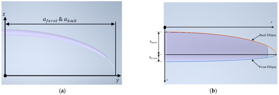
Figure 8.
Half of (a) front view and (b) top view of the utilised parakite with the respective coordinate system and both back and front ellipse marked on the top view. afront and aback are the major radius while bfront and bback are the minor radius.
This study evaluates multiple parameters; therefore, the ellipse span geometry in the - plane is defined by Equation (34), which can be scaled using a factor for future calculations. The parakite presented by D. Lamartiniere et al. [29] has an overall span of 220 m, which was scaled down by a factor of 0.69 to achieve a wingspan equal to 1.2 times the rotor diameter. Additionally, the chord length variation along the x-direction is described by elliptical Equations (35) and (36), with their combined effect represented by Equation (37). Equations (35) and (36) utilise and , where these are the major and minor elliptical radii dimensions, respectively, for the ellipses making up the parakite as depicted in Figure 8. Figure 9 depicts the span ratio of the kite to the wind turbine along with its height.
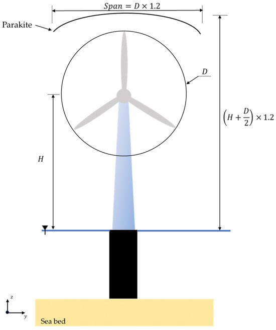
Figure 9.
Representation of the parakite span and corresponding height determination.
The baseline parameters defining the environmental, structural, and geometric conditions applied throughout this study are tabulated by Table 2. It also represents the basic Parakite data, such as the geometric properties and lifting gas. During this study, a wind shear exponent of 0.06 was assumed since the OWT is placed in open, calm sea [31]. The cable diameter of 0.019 m, as shown in Table 2, was determined by subjecting the wind turbine to a maximum wind speed of 24 m/s and sizing the cable to withstand 2.8 times the expected load, corresponding to a safety factor of 2.8 relative to the cable’s tensile strength.
Table 2.
Baseline modelled conditions and parameters inputted into the Python code (n/a—non applicable).
The code was configured to perform multiple simulation runs by systematically varying several key parameters: number of cable discretisation nodes, cable weight, wind speed, parakite geometry, and cable length, as presented in Figure 10. The number of cable discretisation nodes was varied from 10 to 8500 nodes to analyse its influence on the final result. The discretisation results are further analysed through Equations (38) and (39), where the bending moment reduction and shear increase in the coarser discretisation is compared to the finer one. Cable weight was adjusted from 0.27 kg/m to 100 kg/m, with the initial value corresponding to a cable diameter of 19 mm. These simulations were conducted with the expectation that the resulting cable shape would follow a catenary profile.
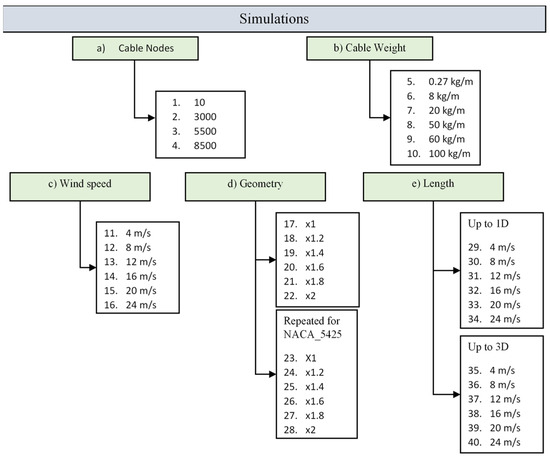
Figure 10.
Simulations carried out throughout this study; (a,b) were carried out for numerical discretisation error assessment, while (c–e) were carried out for final analysis.
The horizontal displacement of the cable, driven by drag forces acting on both the parakite and the cable for increasing wind speeds, was investigated. Geometry variations involved adjusting the values of parameters afront, and aback. bfront and bback presented in Figure 8 and also in Equations (33) and (34), were scaled relative to the original Parakite dimensions. The lift and drag forces for geometry scaling factor () from ×1.2 to ×2 were analysed with respect to the values at of ×1 using Equations (40) and (41). This same geometric variation procedure was also applied to a parakite cross-section based on the NACA 5425 aerofoil, which was previously investigated by D. Lamartinière et al. [29].
In addition, the cable length was varied such that its downstream reach from the anchoring point remained within a range of 1D to 3D horizontally, while its vertical extent was maintained at 1.2 times the rotor hub height. All the mentioned simulations are presented in Figure 10.
For the cable length variation study, the lengths were determined based on two key parameters: first, the parakite’s height was set to be 1.2 times the height of the rotor tip; second, the parakite was allowed to deflect either 1D or 3D downstream, where D represents the rotor diameter. This relationship is illustrated in Figure 11.
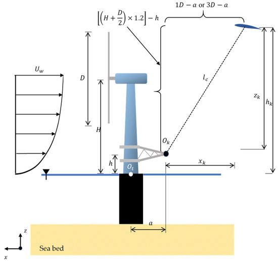
Figure 11.
Offshore wind turbine coupled with Parakite, indicating the determination of the parakite’s cable length.
For a downstream deflection of 1D, the required cable length was approximately 194.1 m, whereas for a 3D deflection, the cable length increased to 373.5 m. These calculations were made under the assumption that the cable extends in a straight line from the rotor to the parakite. Furthermore, these lengths were subjected to different wind speeds to analyse the cable profile.
4.1. Numerical Discretisation Error
A numerical discretisation error analysis was conducted to evaluate the code’s performance under varying conditions. These will be analysed through the following subsections.
4.1.1. Cable Nodes
Prior to conducting the main simulations, a sensitivity analysis was performed on the number of nodes used to model the parakite cable, varying from 10 to 8500 nodes as shown in Table 3. These simulations were carried out with the parameters presented in Table 2. The results indicate that variations in node count have a negligible effect on the output values, including both the decrease in bending moment and the increase in shear force. When comparing to coarse cable discretisation to the finer 8500-node configuration, the percentage differences remain minimal, as computed through Equations (36) and (37). Additionally, the computational time was found to be largely unaffected by the number of nodes.
Table 3.
Bending moment decrease (%) and shear increase (%) code output value and percentage change in moment and shear with respect to 8500 nodes while indicating code execution duration.
The cable profiles generated by the in-house Python code reveal that, regardless of the number of nodes used, the overall shape remains consistent, as shown in Figure 12a. A closer inspection of the parakite region in Figure 12b highlights that the profiles for 3000, 5500, and 8500 nodes are nearly identical. In contrast, the profile obtained using only 10 nodes deviates noticeably from the others, indicating reduced accuracy at low discretisation levels. From this analysis, it can be concluded that increasing the number of nodes beyond a certain threshold yields negligible differences in the predicted cable profile. The simulations results presented in the following sections were derived using 8500 cable nodes.
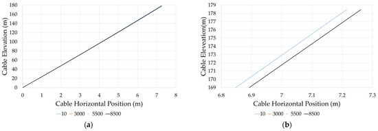
Figure 12.
Cable profile for (a) full cable length and (b) close-up for cable discretisation of 10, 3000, 5500, and 8500 nodes. (0,0) is the anchoring point of the cable to the horizontal strut (Ok).
4.1.2. Cable Weight
To qualitatively validate the cable model (Figure 4) and ensure that it produced realistic results, simulations were performed for different prescribed cable weights while retaining a fixed cable diameter. As shown in Figure 10 condition (b), the cable weight was varied from 0.27 kg/m to 100 kg/m. The parameters listed in Table 2 were held constant throughout the study. Figure 13a demonstrates that increasing the cable weight leads to greater sagging, particularly in the mid-span region, and causes the cable to be at a more horizontal orientation. Additionally, Figure 13b illustrates that at higher cable weights, the code is capable of capturing a realistic catenary profile. These findings confirm that the developed code effectively replicates real-world behaviour under varying cable weight conditions since greater load causes the cable to sag.
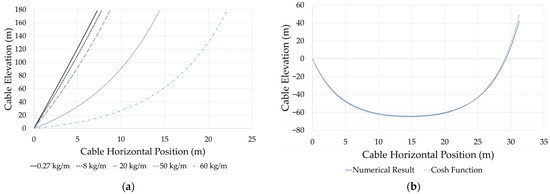
Figure 13.
Cable profile for (a) cable weight at 0.27 kg/m, 8 kg/m, 20 kg/m, 40 kg/m, and 60 kg/m and (b) for cable with a weight of 100 kg/m and while comparing it to the cosh function. (0,0) is the anchoring point of the cable to the wind turbine horizontal strut (Ok).
When comparing the cable profile corresponding to a weight of 0.27 kg/m of Figure 13a with an idealised straight-line profile defined by Equation (42), the variation in displacement along the cable is found to range from approximately +1% to −3%. This minor deviation confirms that, under such low self-weight conditions, the cable remains nearly linear, with minimal sagging effects given that a light fibre-type cable is considered.
The catenary cable profile exhibited by Figure 13b can be theoretically described by a hyperbolic cosine function, represented in the same figure and expressed by Equation (43). The fitted curve indicates a maximum deflection differing by 15% from that calculated through the Python code. This disparity is primarily attributed to the numerical approximation errors which are amplified given that the cable is nearly linear, with very limited curvature.
5. Results and Discussion
A parametric study was carried out considering three primary parameters: free-stream wind speed, parakite geometry, and cable length. The influence of each parameter on the system performance is analysed in the following section.
5.1. Wind Speed Variation
The results in this section are based on the parameter values outlined in Table 2, with windspeed varied from 4 m/s to 24 m/s, in increments of 4 m/s. As illustrated in Figure 14a, increasing the wind speed results in a significant reduction in the bending moment at the tower base, accompanied by a corresponding—though comparatively modest—increase in shear force.
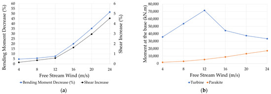
Figure 14.
(a) Bending moment decrease and shear increase (%) with free-stream wind speed, and (b) comparison of the bending moments at the tower base induced by the wind turbine and by the parakite at different free-stream wind speeds.
Comparing Figure 14a to Figure 6 reveals a strong correlation between the reduction in bending moment and the rotor thrust. Specifically, as wind speed increases from 0 m/s to 12 m/s, rotor thrust rises from 200 kN to 800 kN. Beyond 12 m/s, however, the rotor thrust begins to decline, impacting the rate at which the bending moment decreases. As a result, the bending moment reduction gradient is more gradual between 4 m/s and 12 m/s, and becomes steeper from 12 m/s to 24 m/s.
Figure 14b complements the trends observed in Figure 14a by providing a direct comparison of the bending moments acting at the tower base due to the turbine thrust and the parakite moment across varying wind speeds. The plot shows that the turbine moment increases with wind speed up to the rated condition of 12 m/s, where the rotor thrust reaches its maximum, and subsequently decreases beyond this point as the turbine begins to regulate its power output. This variation in the turbine moment directly explains the pattern seen in Figure 14a, where the percentage reduction in tower bending moment becomes more pronounced at higher wind speeds when the turbine’s own thrust decreases but the parakite’s moment continues to increase.
Independently, Figure 14b reveals that the parakite generates a steadily increasing counter moment with wind speed, reflecting its growing aerodynamic lift. While the turbine moment peaks at around 12 m/s and then declines, the parakite moment exhibits an increase, reaching its highest value at 24 m/s. This opposing trend demonstrates the parakite’s effectiveness in partially compensating for the rotor-induced bending moment, resulting in the significant reductions ~51% shown in Figure 14a.
In addition to the previous analysis, examination of Figure 15a reveals that increasing wind speeds lead to greater horizontal deflection of the parakite, which in turn significantly influences the behaviour of the mooring cable. The highest value of each plot denotes the location of the parakite. As the wind speed increases, the horizontal displacement of the cable increases steadily, which is clearly illustrated by the progression of the curves on the graph. For instance, at 24 m/s, the cable exhibits the greatest horizontal displacement reaching more than 8 m compared to approximately 3 m at just 4 m/s. This trend highlights a non-proportional relationship between wind speed and cable displacement, suggesting that the aerodynamic forces on the parakite amplify with wind velocity, thereby exerting increased lateral force on the cable system. Furthermore, the cable elevation is further highlighted by the table in Figure 15b.
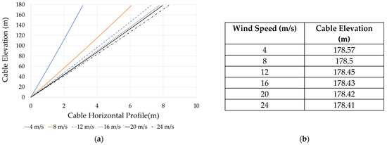
Figure 15.
(a) Cable profile for wind speeds from 4 m/s to 24 m/s, in steps of 4 m/s. (0,0) is the anchoring point of the cable to the wind turbine horizontal strut (Ok). (b) Wind speed and the respective cable elevation (m).
For a system in which the mass of the parakite and cable are negligible, the cable would follow a straight line with an inclination equal to .
The cable inclination estimated by this approximation was compared with that derived from Figure 15 for a wind speed of 4 m/s and only a percentage deviation of 0.11% was noted. This is due to the fact that the total lift force is significantly larger than the overall weight of the parakite–cable assembly.
The developed code is structured to optimise the aerodynamic performance of the parakite by maximising the lift-to-drag ratio (/) determined by the AVL code. The optimal angle of attack was found to remain constant and equal to 0.8° across the modelled windspeed range. Operating at this condition enhances lift generation while minimising drag-induced energy losses. However, since the correction for viscous drag effects is applied to the parakite aerodynamics only after the AVL computation (see Section 2.2), the selected angle of attack deviates from the true optimum corresponding to the maximum achievable lift-to-drag ratio. Nevertheless, this approximation is considered sufficient for the present preliminary study, as it provides a close-to-optimal operating point that yields high aerodynamic performance while maintaining stable, attached flow conditions. Moreover, considering the base study of Table 2, it was noted that the drag induced by the cable is approximately 0.2% that of the parakite.
5.2. Geometry Variation
To examine the influence of altering the parakite geometry, the width of the parakite was maintained constant; that is, the major radii of the front and back ellipse ( and ), depicted in Figure 8a, remained constant through this study. In the meantime, the minor circle radii was varied from ×1 up to ×2 in steps of ×0.2 both for the back and front ellipse and , respectively. In addition to this analysis, the aerofoil profile was varied from the NACA 4412 to the NACA5425, where the latter cross-section is presented in Figure 16. Unless specified otherwise, the remaining parameter values were retained as fixed and are presented in Table 2.
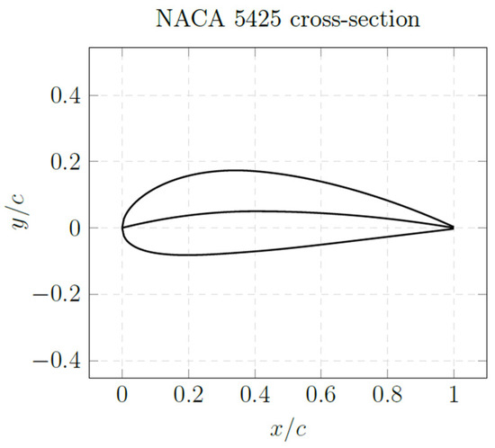
Figure 16.
NACA5425 aerofoil cross-section [29].
An initial analysis of the forces induced by the kite, using the corresponding geometry scaling factors from Table 4, indicates that an increase in the geometric scale leads to a proportional increase in both lift and drag forces. A detailed evaluation of the percentage change between a scaling factor of 1 and subsequent increments reveals a gradual rise in force magnitudes as analysed through Equations (40) and (41). Specifically, the drag force increases by approximately 19% to 89%, while the lift force exhibits an increase ranging from 19% up to 100%. An examination of the lift-to-drag ratio in Table 4 reveals that, despite increases in both lift and drag, the ratio itself remained constant irrespective of .
Table 4.
Drag (D) and lift (L) force with respective geometry scaling factor (Sf), along with the percentage change on drag (δD) and lift (δL) with respect to a scaling factor of 1 while indicating the lift-to-drag ratio.
Further to the previous analysis, Figure 17 demonstrates that an increased geometry scaling factor significantly contributes to a reduction in bending moment and an increase in shear force. Furthermore, regardless of the geometry scaling factor, the decrease in bending moment consistently exceeds the corresponding increase in shear force.
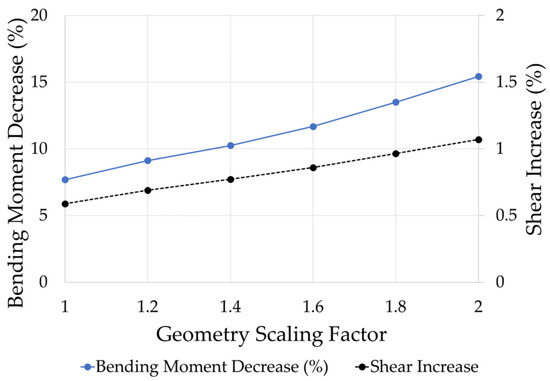
Figure 17.
Bending moment decrease (%) and shear increase (%) against the geometry scaling factor of the parakite (Sf) for NACA 4412.
Figure 18a illustrates the vertical and horizontal displacements of the cable under varying geometry scaling factors. Despite the application of different lift and drag forces, the resulting cable displacements remained minimal. Additionally, Figure 18b shows that the horizontal deflection is not expected to exceed 1.2 m.
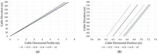
Figure 18.
Cable profile for (a) complete cable and (b) close-up with different geometry scaling factor for NACA4412. (0,0) is the anchoring point of the cable to the wind turbine horizontal strut (Ok).
The previous results can be further interpreted by comparing the lift coefficient against the angle of attack for the different aerofoils under investigation. As shown in Figure 19a, under the same scaling factor of ×2 applied to both geometries, the parakite with the NACA 5425 aerofoil consistently demonstrates the highest lift coefficient across all angles of attack. Additionally, Figure 19b shows that NACA 5425 also experiences a higher drag coefficient compared to NACA 4412. These variations in aerodynamic performance strongly support the earlier discussion regarding the observed decrease in bending moment and the corresponding increase in shear force.
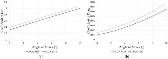
Figure 19.
(a) Coefficient of lift and (b) coefficient of drag against angle of attack (α) for NACA 4412 and NACA 5425, with a scaling factor of ×2.
Figure 20a,b illustrate that the bending moment decrease and shear increase for the NACA 5425 exhibit a more consistent trend, whereas the NACA 4412 shows a less uniform behaviour. It is also evident that irrespective of the aerofoil type, the bending moment decrease was much more than the exhibited shear increase. From this analysis, it could also be concluded that greater forces were exerted by the parakite with the NACA 5425 profile, both for lift and drag.
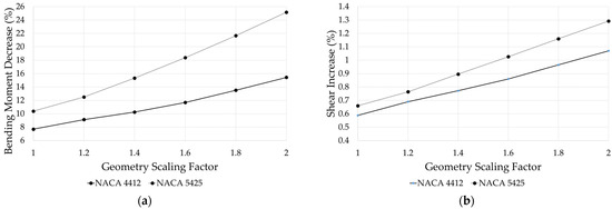
Figure 20.
(a) Bending moment decrease (%) against geometry scaling factor and (b) shear increase (%) against geometry scaling factor.
The cable profiles corresponding to the two extreme geometry scaling factors, as shown in Figure 21a,b, and illustrate the displacement behaviour at scaling factors of ×1 and ×2, respectively. It is observed that for both scaling factors, the cable subjected to the NACA 4412 aerofoil exhibits greater horizontal displacement compared to the NACA 5425. This indicates that the NACA 5425 generates a higher aerodynamic lifting force, which in turn results in less pronounced cable deflection. The effect becomes more noticeable at the larger scaling factor of ×2, where the displacement difference between the two aerofoils increases. This behaviour is primarily attributed to the greater lift and drag forces experienced by the parakite equipped with the NACA 5425 profile, enhancing its horizontal deflection and overall aerodynamic performance.
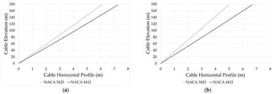
Figure 21.
Cable profile (a) geometry scaling factor of ×1 and (b) geometry scaling factor of ×2. (0,0) is the anchoring point of the cable to the wind turbine horizontal strut (Ok).
The internal volume of the parakite configured with the NACA 5425 profile is approximately twice that of the parakite with the NACA 4412. While the NACA 4412-based parakite exhibits an aerodynamic lift-to-drag coefficient ratio CL/CD of 29.71 and a L/D of 27.26, the NACA 5425 variant delivers an aerodynamic CL/CD of 26.13 but a higher L/D of 36.45. Even though NACA 5425’s CL/CD is marginally lower, its inflated internal volume enhances buoyancy, thereby reducing horizontal deflection more effectively. This larger volume therefore plays a key role in stability and performance beyond what the aerofoil coefficient metrics alone would predict. Consequently, the interpretation of horizontal deflection behaviour must account for both aerodynamic coefficient ratios and the buoyancy internal volume when comparing the two air foil configurations.
5.3. Cable Length Variation
This analysis was conducted to evaluate the position of the parakite under different wind speeds and cable lengths. As shown in Figure 22a, the horizontal deflection of the cable remains below 18.5 m across all tested conditions, regardless of wind speed or cable length. Specifically, even at a high wind speed of 24 m/s and with the longest cable length of 373.5 m (corresponding to a 3D downstream positioning), the cable does not exceed this horizontal displacement limit. Therefore, in the case of situating a wind turbine 1D downstream and employing a cable of 373.5 m, the parakites will still be a considerable distance upstream from the downstream turbine. Furthermore, the cable elevation was minimally influenced as exhibited by Figure 22b.
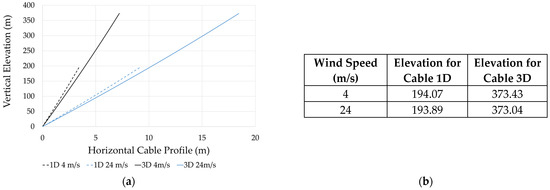
Figure 22.
(a) Cable profile for a parakite moored with a cable length of 194.1 m and 373.5 m. (0,0) is the anchoring point of the cable to the wind turbine horizontal strut (Ok). (b) Cable elevation for the two lengths under study with respect to the wind speed.
It could be observed from Figure 23a,b that if a parakite utilises a cable of 373.5 m, it would have minimal influence on both the bending moment decrease and the shear increase, irrespective of the free stream wind speed. Irrespective of the cable length, the bending moment decrease is always greater than the shear increase. The influence of the cable length should further be analysed while considering the aerodynamic influence of the wind turbine with respect to the parakite.
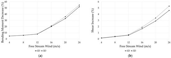
Figure 23.
(a) Bending moment decrease (%) against free stream wind (m/s) and (b) shear increase (%) against free stream wind (m/s).
6. Conclusions
This article delved into detail and analysed a novel system of an OWT coupled with a lighter-than-air parakite. Through the in-house-developed Python code, the conclusions could be drawn as follows:
- The proposed concept (Figure 1) demonstrates a significant reduction in the bending moments acting at the base of the OWT tower. The lift generated by the parakite produces a counteracting moment opposing that induced by the rotor thrust, thereby reducing compressive and tensile stresses at the tower base. The overall structural impact is positive, as the moment reduction is achieved with only a marginal increase in shear force. It was estimated that the tower bending moment decreased by 7.7% at the rated wind speed, where the rotor thrust is at its maximum, while the corresponding shear force increased by 0.6%. At higher wind speeds, where the magnitude of the rotor thrust decreases, the percentage reduction in bending moment gradually increases to 51.7% at a wind speed of 24 m/s, with the corresponding shear force increasing by only around 4.6%. These finding provide a strong motivation for further exploration of the concept.
- For both NACA 4412 and NACA 5425 profiles, larger geometric scaling factors yielded higher lift and drag forces and thus greater tower bending moment reduction. The NACA 5425 parakite consistently produced higher lift coefficients (≈10–15% greater), leading to improved parakite performance compared with NACA 4412
- Varying the cable length between 194.1 m and 373.5 m had minimal impact on the reduction in bending moment and the increase in shear force
Although the present study has demonstrated the potential of the proposed mooring approach of a parakite to reduce wind turbine bending moments at the tower base, further investigations are warranted. In particular, more advanced Computational Fluid Dynamics (CFD) simulations are required to assess the effectiveness of the concept in augmenting wind flow and to provide more reliable estimates of the induced aerodynamic loads on the turbine tower. In realistic operating conditions, the parakite will be subjected to complex wind turbine wake effects, including wake shear, velocity deficits, and unsteady turbulent structures. These effects may alter the parakite’s geometry and effective angle of attack, and consequently influence its aerodynamic response, position, and induced forces on the tower. As part of future work, high-fidelity CFD and aeroelastic simulations will be carried out to model the wake–parakite flow interactions and assess how unsteady inflow conditions affect the parakite geometry, loading, and altitude. These studies could be complemented by wind-tunnel experiments on a scaled wind turbine–parakite assembly. Future work should quantify the sensitivity of parakite-induced loads to meteorological conditions (e.g., atmospheric temperature and stability) and systematically assess the impact of alternative parakite aerofoil geometries on lift–drag characteristics and resulting tower-base loads. Future work will also investigate operation at maximum lift to assess its influence on tower bending-moment reduction and shear loading. In addition, structural dynamic analyses are necessary to evaluate the overall impact of parakite-induced dynamic loads on the complete wind turbine system under realistic unsteady wind conditions, including turbulence.
Author Contributions
Conceptualization, L.J.B., K.Z., T.S. and J.-P.M.; methodology, L.J.B., K.Z., T.S. and J.-P.M.; software, L.J.B.; validation, L.J.B.; formal analysis, L.J.B.; investigation, L.J.B. and K.Z.; resources, T.S. and J.-P.M.; data curation, L.J.B. and K.Z.; writing—original draft preparation, L.J.B.; writing—review and editing, T.S., K.Z. and L.J.B.; visualization, L.J.B.; supervision, T.S. and J.-P.M.; project administration, T.S.; funding acquisition, T.S. All authors have read and agreed to the published version of the manuscript.
Funding
The work presented in this paper forms part of the ParaWIND project which is being financially supported by XjenzaMalta under the Research Excellence Program 2024 (Project Reference: REP-2024-003).
Data Availability Statement
Data are contained within the article.
Conflicts of Interest
The authors declare no conflicts of interest.
Abbreviations
The following abbreviations are used in this manuscript:
| AOA | Angle of Attack |
| AVL | Athena Vortex Lattice |
| MIT | Massachusetts Institute of Technology |
| NREL | National Renewable Energy Laboratory |
| OWT | Offshore Wind Turbine |
| RES | Renewable Energy Sources |
| VLM | Vortex Lattice Method |
References
- Castelino, R.V.; Kumar, P.; Kashyap, Y.; Karthikeyan, A.; Sharma, K.M.; Karmakar, D.; Kosmopoulos, P. Exploring the Potential of Kite-Based Wind Power Generation: An Emulation-Based Approach. Energies 2023, 16, 5213. [Google Scholar] [CrossRef]
- Olabi, G.; Wilberforce, T.; Elsaid, K.; Sayed, E.T.; Salmeh, T.; Abdelkarem, M.A.; Baroutaji, A. A Review on Failure Modes of Wind Turbine Components. Energies 2021, 14, 5241. [Google Scholar] [CrossRef]
- Liu, X.; Lu, C.; Li, G.; Godbole, A.; Chen, Y. Effects of aerodynamic damping on the tower load of offshore horizontal axis wind turbines. Appl. Energy 2017, 204, 1101–1114. [Google Scholar] [CrossRef]
- Bonou, A.; Laurent, A.; Olsen, S.I. Life cycle assessment of onshore and offshore wind energy-from theory to application. Appl. Energy 2016, 180, 327–337. [Google Scholar] [CrossRef]
- Carswel, W.; Johansson, J.; Lovhalt, F.; Madshus, C.; DeGroot, D.; Myers, A. Foundation damping and the dynamics of offshore wind turbine monopiles. Renew. Energy 2015, 80, 724–736. [Google Scholar] [CrossRef]
- Seidel, M. Substructures for offshore wind turbines-Current trends and developments. In Festschrift Peter Schaumann; Leibniz Universität Hannover: Hannover, Germany, 2014; pp. 363–368. [Google Scholar] [CrossRef]
- Rezaei, F.; Contestabile, P.; Vicinanza, D.; Azzellino, A. Towards understanding environmental and cumulative impacts of floating wind farms: Lessons learned from the fixed-bottom offshore wind farms. Ocean Coast. Manag. 2023, 243, 106772. [Google Scholar] [CrossRef]
- IRENA; CPI. Global Landscape of Renewable Energy Finance; International Renewable Energy Agency: Abu Dhabi, United Arab Emirates, 2020. [Google Scholar]
- Díaz, H.; Soares, C.G. Review of the current status, technology and future trends of offshore wind farms. Ocean Eng. 2020, 209, 107381. [Google Scholar] [CrossRef]
- Chen, J.; Kim, M.-H. Review of Recent Offshore Wind Turbine Research and Optimization Methodologies in Their Design. Mar. Sci. Eng. 2022, 10, 28. [Google Scholar] [CrossRef]
- Porté-Age, F.; Bastankhah, M.; Shamsoddin, S. Wind-Turbine and Wind-Farm Flows: A Review. Bound.-Layer Meteorol. 2020, 174, 1–59. [Google Scholar] [CrossRef]
- Warder, S.C.; Pigott, M.D. The future of offshore wind power production: Wake and climate impacts. Appl. Energy 2025, 380, 124956. [Google Scholar] [CrossRef]
- Barthelmie, R.; Pryor, S.C.; Frandsen, S.T.; Hansen, K.S. Quantifying the Impact of Wind Turbine Wakes on Power Output at Offshore Wind Farms. J. Atmos. Ocean. Technol. 2010, 27, 1302–1317. [Google Scholar] [CrossRef]
- Gupta, N. A review on the inclusion of wind generation in power system studies. Renew. Sustain. Energy Rev. 2016, 59, 530–543. [Google Scholar] [CrossRef]
- Boonman, D.; Broich, C.; Deerenberg, R.; Groot, K.; Hamraz, A.; Kalthof, R.; Nieuwint, G.; Chneiders, J.; Tang, Y.; Wiegernik, J. Wind Farm Energy: Design Synthesis Exercise Spring 2011. Group S12: Final Report (Student Report). 2011. Available online: https://repository.tudelft.nl/record/uuid:9ec5078c-c02a-43db-99b9-00bde8871b58 (accessed on 28 June 2011).
- Zhang, K.; Hayostek, S.; Amitay, M.; He, W.; Theofilis, V.; Taira, K. On the formation of three-dimensional flows over finite-aspect-ratio wings under tip effects. J. Fluid Mech. 2020, 895, A9. [Google Scholar] [CrossRef]
- He, K.; Ye, J. Dynamics of offshore wind turbine-seabed foundation under hydrodynamic and aerodynamic loads: A coupled numerical way. Renew. Energy 2023, 202, 453–469. [Google Scholar] [CrossRef]
- Lee, Y.-S.; Choi, B.-L.; Lee, J.H.; Kim, S.Y.; Han, S. Reliability-based design optimisation of monopile transition piece for offshore wind turbine system. Renew. Energy 2014, 71, 729–741. [Google Scholar] [CrossRef]
- Lee, Y.-S.; Gonzalez, J.A.; Lee, J.H.; Kim, Y.I.; Park, K.; Han, S. Structural topology optimisation of the transition piece for an offshore wind turbine with jacket foundation. Renew. Energy 2016, 85, 1214–1225. [Google Scholar] [CrossRef]
- CoolProp. Welcome to CoolProp. CoolProp. Available online: https://coolprop.org/ (accessed on 24 July 2025).
- Sun-Mach, S.; Minnis, P.; Chen, Y.; Kato, S.; Yi, Y.; Gibson, S.C.; Heck, P.W.; Winker, D.M. Regional Apparent Boundary Layer Lapse Rates Determined from CALIPSO and MODIS Data for Cloud-Height Determination. J. Appl. Meteorol. Climatol. 2013, 53, 990–1011. [Google Scholar] [CrossRef]
- Budziak, K. Aerodynamic Analysis with Athena Vortex Lattice (AVL); Department of Automotive and Aeronautical Engineering—Hamburg University of Applied Sciences: Hamburg, Germany, 2015. [Google Scholar]
- Drela, M.; Youngren, H. AVL. MIT. Available online: https://web.mit.edu/drela/Public/web/avl/ (accessed on 24 July 2025).
- White, F.M. Fluid Mechanics, 7th ed.; WCB McGraw-Hill: New York, NY, USA, 2011. [Google Scholar]
- Song, L.; Fu, S.; Dai, S.; Zhang, M.; Chen, Y. Distribution of drag force coefficient along a flexible riser undergoing VIV in sheared flow. Ocean Eng. 2016, 126, 1–11. [Google Scholar] [CrossRef]
- Schlichting, H.; Gersten, K. 1.6 Comparison of Measurements Using the Inviscid Limiting Solution. In Boundary-Layer Theory, 9th ed.; Springer: Berlin, Germany, 2017; pp. 14–26. [Google Scholar]
- Jonkman, J.; Butterfield, S.; Musial, W.; Scott, G. Definition of a 5-MW Reference Wind Turbine for Offshore System Development; No. NREL/TP-500-38060; National Renewable Energy Lab. (NREL): Golden, CO, USA, 2009.
- Shubov, M.V. Feasibility of Extremely Heavy Lift Hot Air Balloons and Airships. Phys. Sci. Biophys. J. 2022, 6, 1–8. [Google Scholar] [CrossRef]
- Lamartiniere, D.; Sphon, A.; Sant, T. Modeling the Aerodynamic Loads of a Wing-Shaped Kite Using CFD; Engineer Internship Report; University of Malta: Msida, Malta, 2024. [Google Scholar]
- Sonawane, B.S.; Fernandes, M.A.; Pant, V.; Tandale, M.S.; Pant, R.S. Material Characterization of Envelope Fabrics for Lighter-Than-Air Systems. In International Colloquium on Materials, Manufacturing and Metrology; IIT Madras: Chennai, India, 2014. [Google Scholar]
- Visich, A.; Conan, B. Measurement and analysis of high altitude wind profiles over the sea in a coastal zone using a scanning wind LiDAR—Application to wind energy. Wind Energy Sci. Discuss. 2023, 325, 120749. [Google Scholar] [CrossRef]
- Mat Web-Material Propery Data. Toyobo Dyneema® SK60 High Strength Polyethylene Fiber. Mat Web- Material Propery Data. Available online: https://matweb.com/search/datasheet.aspx?matguid=4481722d60e54cc3b3c112eb3d4b9d02&ckck=1 (accessed on 29 July 2025).


Disclaimer/Publisher’s Note: The statements, opinions and data contained in all publications are solely those of the individual author(s) and contributor(s) and not of MDPI and/or the editor(s). MDPI and/or the editor(s) disclaim responsibility for any injury to people or property resulting from any ideas, methods, instructions or products referred to in the content. |
© 2026 by the authors. Licensee MDPI, Basel, Switzerland. This article is an open access article distributed under the terms and conditions of the Creative Commons Attribution (CC BY) license.