Abstract
With the rising demand for renewable hydrogen as an alternative sustainable fuel, efficient transport strategies have become essential, particularly for regional and small-scale applications. While most previous studies focus on the long-distance transport of hydrogen, little attention has been given to the application in regions that are remote from major transmission infrastructure. This study evaluates the techno-economic performance of hydrogen road transport using multiple-element hydrogen gas containers and compares it with multimodal transport using rail. The comparison is performed for the southeastern region of the Czech Republic. The comprehensive techno-economic assessment incorporates detailed technical evaluations, precise fuel and energy consumption calculations, and real-world infrastructure planning to enhance accuracy. Results showed that multimodal transport of hydrogen can significantly reduce the cost for distances exceeding 90 km. The cost is calculated based on annual vehicle utilization, assuming the remaining utilization will be allocated to other tasks throughout the year. However, the cost-effectiveness of rail transportation is influenced by track capacity limits and possible delays. Additionally, this study highlights the crucial role of regional logistics hubs in optimizing transport modes, further reducing costs and improving efficiency.
1. Introduction
Hydrogen has gained increasing attention in recent years thanks to its versatility as a raw material, fuel, and energy carrier. Its primary applications span industry, transport, energy, and construction. A key advantage of hydrogen as an energy source is that it does not release CO2 and has minimal air pollution impact. This makes it a highly promising alternative in sectors where reducing carbon emissions is challenging with more conservative options. Another great advantage of hydrogen is its high lower heating value of 120 MJ/kg, compared to natural gas (47.1 MJ/kg in the US market), LNG (48.6 MJ/kg), bituminous coal (29 MJ/kg), and diesel (42.6 MJ/kg) [1].
One of the most critical applications of hydrogen lies in the energy sector. In the European Union (EU), renewable electricity is expected to decarbonize a substantial share of energy consumption by 2050 [2]. Hydrogen is considered an essential component in this transition, particularly for renewable energy storage, complementing batteries. Hydrogen can also replace fossil fuels in energy-intensive processes such as the steel and chemical industries. Another important application of hydrogen is in the transportation sector. While electricity and batteries are central to the decarbonization strategies, hydrogen may offer a viable alternative for road freight transport or rail transport on non-electrified lines.
Global hydrogen demand has been growing for decades. According to the International Energy Agency [3], global hydrogen demand reached 97 Mt in 2023 with an annual increase rate of 2.5%. More than half of the hydrogen (54 Mt) was used in the industry, mostly for ammonia, methanol, and steel production, while 43 Mt was consumed in refining. The demand for transportation was only 60 kt in 2023, accounting for less than 0.1% of global consumption. However, this value increased sharply by around 55% compared to 2022.
The potential applications of hydrogen in the future are extensive, but large-scale applications will depend on the ability to transport it efficiently from production sites to consumers, including rural areas. This paper focuses on the technical, economic, and environmental aspects of hydrogen transportation, specifically within the context of the Czech Republic.
In the Czech Republic, approximately 125,000 tons of hydrogen are produced and consumed annually, primarily from fossil sources [4]. Most of the produced hydrogen is used in the chemical industry, typically at the site of its production. Occasionally, pilot projects involving hydrogen-fueled trucks and buses are carried out in various cities, and six filling stations are currently in operation in the Czech Republic. Among these stations, three are public, the other three are private. In addition, another two stations are under construction [5]. These stations rely on road transport for hydrogen delivery in gaseous form, but further details on the supply chain remain unavailable. Considering the potential of hydrogen as a clean energy source, its demands are expected to increase within the Czech Republic. Hydrogen transportation within shorter distances would become critical to ensure the overall sustainable use of hydrogen.
In this study, a literature review was first carried out to summarize the state-of-the-art of hydrogen logistics, transportation methods, techno-economic evaluation models, and related challenges. Based on these insights and an analysis of the identified challenges, a techno-economic assessment (TEA) model is developed. The model is then applied in a case study focusing on selected regions in the Czech Republic, evaluating the technical and economic performances of hydrogen transportation via road and multimodal transport. This study builds upon our previous work, where the TEA model was initially introduced [6], by significantly expanding its scope, structure, assessment methods, and application.
This study serves as an initial attempt to investigate the technical, economic, and environmental aspects of hydrogen transportation within short distances, offering insights and guidance for the further management of hydrogen logistics in the Czech Republic. Additionally, the proposed model is designed as a flexible framework that can be adapted and extended for broader applications. By incorporating key parameters and real-world constraints into the model, it enables a more accurate evaluation of hydrogen distribution strategies, supporting informed decision-making in both policy and industry.
2. Literature Review
The literature mainly focuses on the development phase of different hydrogen transportation methods and compares their advantages and disadvantages. The current state of existing technical and economic assessment of short to medium-distance hydrogen transportation is also provided with a focus on rail and multimodal transport.
2.1. Pipelines
Approximately 5000 km of hydrogen pipelines are currently in operation worldwide, mainly in the United States and Europe [3]. Europe accounts for around 1500 km of this network [7]. These pipelines are mostly privately owned and connect refineries and chemical complexes. Constructing a dedicated hydrogen pipeline is the most technologically optimal, as it allows for design in full compliance with relevant standards and specifications. However, the high construction costs make this option financially demanding.
An alternative is to repurpose existing natural gas pipelines for hydrogen transport. With natural gas in the EU expected to decline after 2030, portions of infrastructure could be converted for large-scale, cross-border hydrogen transport [2]. According to the International Energy Agency [3], Germany plans to complete its hydrogen core network by 2032, spanning 9700 km, with 60% consisting of repurposed natural gas pipelines.
There are two approaches to utilizing existing gas networks: mixing hydrogen with natural gas or fully replacing natural gas with hydrogen. The latter solution is more cost-effective, as it leverages existing infrastructure while avoiding additional investments in mixing and separation stations. However, direct replacement is not straightforward due to hydrogen’s unique properties. Particularly, its small molecular size can increase the risk of leakage. Additionally, carbon steel used in gas pipelines is susceptible to hydrogen embrittlement and cracking [8].
Hydrogen blending, the practice of mixing hydrogen with natural gas, is considered an interim solution until more efficient alternatives are available or investment risks decrease with the rising hydrogen demand. Currently, blending is primarily used with fossil-based hydrogen at low concentrations (around 2%). Several gas network operators are testing the safe hydrogen blending limits for their infrastructure. These projects do not separate the hydrogen at the endpoint, instead, the mixed gas is delivered directly to the customers.
A study by the Confederation of Industry of the Czech Republic [9] found that up to 20% of hydrogen can be blended into the Czech gas pipeline network without requiring modifications. Similarly, GasNet, the country’s largest natural gas distributor, cited German test results indicating that a 20% hydrogen blend does not necessitate a technical adjustment to end-user devices [10]. The company has also begun injecting 10% hydrogen, produced via an electrolyzer with wind energy, into the gas network in a town named Hranice u Aše in the western Czech Republic [11].
Currently, increasing attention has been given to deblending technology. However, only a limited number of demonstrations and tests have been conducted, suggesting that the technology is not yet mature enough for large-scale implementation [3]. Given its critical role in the hydrogen transport chain, extensive research and development efforts are being directed toward advancing deblending technologies. The most widely studied methods include membrane separation and pressure swing adsorption.
2.2. Road Transport
Pipelines are the most effective method for transporting large hydrogen volumes over long distances. However, for regional distribution or smaller-scale transport, alternative methods—primarily road transport—are necessary.
2.2.1. Gaseous Hydrogen Transport
Hydrogen can be transported by road in liquid and gaseous forms, with gaseous transport being the most discussed option. This method requires the compression of hydrogen to higher pressures, typically between 200 and 500 bar [12] and sometimes up to 700 bar [13]. Higher pressures require more durable pressure vessels, which add weight to the transport unit. However, this weight increase is offset by greater transported hydrogen mass when meeting the legal road vehicle weight limits.
Two main types of semi-trailers are used for hydrogen transport. The first consists of multiple high-pressure cylinders arranged vertically in a cage, often made from carbon fiber-reinforced polymer (Type 4) for greater pressure resistance [14]. The second type is a tube skid with horizontally placed cylindrical tubes—typically up to 10 per trailer, depending on size. While tube skids used to be the dominant solution, vertical cylinder trailers are now more common thanks to their ability to withstand higher pressures, which allows for greater hydrogen transport capacity.
For intermodal transport, the pressure cylinders or tube skids can be mounted in cages designed to fit ISO-standard maritime containers. This configuration, known as a multi-element gas container (MEGC), facilitates seamless transfer between rail and road transport. A notable example is a 20 ft ISO container developed by Vitkovice Cylinders Holding a.s. (Vitkovice Cylinders Holding a.s., Vítkovice 3041, 703 00 Ostrava, Czech Republic) [15], with a working pressure of 300 bars and a storage capacity of 350 kg of hydrogen.
Detailed specifications of hydrogen transport trailers are scarce but are available from some manufacturers, such as Hexagon Purus ASA (Hexagon Purus ASA, Postboks 1353 Vika, 0113 Oslo, Norway) [16]. They produce pressure cylinders and storage solutions ranging from 10 to 45 ft, using vertically aligned compressed cylinders. Table 1 presents the specifications for a 40 ft container from Hexagon Purus, alongside a horizontal tube container from CIMC Enric Holdings Limited (CIMC Enric Holdings Limited, No. 2 Gangwan Avenue, Shekou Industrial Zone, Nanshan District, Shenzhen, Guangdong, China) [17], a Chinese engineering company specializing in natural gas and hydrogen solutions.

Table 1.
Specifications of 40 ft containers for gaseous hydrogen transport; data obtained from [16,17].
The weight of compressed cylinder containers increases significantly as pressure levels rise, particularly when comparing 500 bar to 380 bar. In contrast, the weight of the container with horizontal tubes remains high even at lower pressure levels.
Container cost is a key factor influencing investment costs and subsequent profitability. However, manufacturers do not publicly disclose pricing, making it difficult to estimate costs. Kurz et al. [18] reported the price of a steel tube trailer at around 150,000 USD, while a composite cylinder trailer can cost up to 1 million USD. Reuß et al. [19] used a price of 550,000 EUR in their model for a compressed hydrogen composite trailer with a capacity of 680 kg (pressure level not specified).
2.2.2. Liquid Hydrogen Transport
Liquid hydrogen transportation offers a higher transport volume compared to gaseous hydrogen but brings additional challenges. Hydrogen must be cooled to a cryogenic temperature of −253 °C through an energy-intensive liquefaction process [20], consuming 30–40% of its energy content. However, novel methods such as dual-mixed cryogenic refrigeration show promise in significantly reducing this energy consumption [21].
To maintain these low temperatures, liquified hydrogen needs to be transported in super-insulated cryogenic tanker trucks equipped with pressure-relief systems, typically in spherical and cylindrical [22] designs. These road semi-trailers generally have tank capacities from 30 to 60 m3. Table 2 shows the key parameters of the tank semi-trailer used for liquid hydrogen transportation.
Table 2.
Parameters of the tank semi-trailer for liquid hydrogen transportation; data obtained from [23].
One of the challenges is the boil-off of the liquid hydrogen caused by evaporation due to heat transfer from the ambient [22]. Muhammad [24] stated that boil-off losses in liquid tankers range from 0.3 to 0.6% per day, with additional losses during transfer to storage vessels. Despite these challenges, liquid hydrogen offers significant advances. Its higher energy density compared to gaseous hydrogen, noticeable by transport system weight per 1 MJ of hydrogen, allows for larger transport volumes [20,22]. Additionally, liquid hydrogen also minimizes leakage risks and mitigates hydrogen embrittlement.
2.2.3. Hydrogen Transport with Carriers
Hydrogen carriers are materials or compounds that store and release hydrogen, enabling gaseous hydrogen transport. Commonly used carriers include metal hydrides, ammonia, and liquid organic hydrogen carriers (LOHCs). Metal hydrides such as lithium, sodium, calcium, and magnesium offer high volumetric and gravimetric hydrogen capacities. They form alloys with hydrogen for storage, and hydrogen is later separated by heating the alloy. The spent metal hydride can be transported back to the production facility for reuse.
Ammonia-based hydrogen transport involves combining hydrogen and nitrogen to form ammonia [25]. LOHCs, such as benzene, cyclohexane, or toluene [26], rely on the hydrogenation and dehydrogenation of carbon double bonds. As LOHCs remain liquid at ambient conditions and share properties with crude oil-based liquids, they can be integrated into existing oil infrastructure.
In 2022, the German company Hydrogenious LOHC Technologies tested hydrogen delivery to a refilling station by using LOHC based on benzyl-toluene [27]. Niermann et al. [28] analyzed various hydrogen transport methods from Algeria to Germany, and their results showed that, under the given conditions, methanol is the most cost-effective LOHC option from production to delivery.
While hydrogen carriers seem promising, the technology remains in early development with limited real-world applications. Ongoing research continues to focus on carrier regeneration and the discovery of new materials.
2.3. Rail Transport
Most scientific publications on hydrogen transport focus on pipelines or road trailers, with limited discussion on rail transportation. There is little literature on hydrogen-compatible railway cars, requiring research into developments by railcar manufacturers and operators interested in large-scale transporting hydrogen. For example, DB Cargo is actively promoting hydrogen rail transport in Germany. According to their website [29], viable options include compressed gas tank cars for hydrogen transport carried by ammonia, black steel tank wagons for hydrogen transport carried by methanol, cryo-containers for liquid hydrogen transport, and Multi-Element Gas Containers (MEGCs), similar to those used in road transport.
In 1978, Boeing conducted a study for NASA [30] on railcars for transporting liquefied hydrogen within the Kennedy Space Center for rocket engine use. The resulting design had a capacity of 33,000 gallons (approximately 125 m3). For comparison, Muhammad Aziz [24] noted that a typical rail tank car holds 115 m3 of liquefied hydrogen (approximately 8000 kg).
An interim step toward efficient hydrogen rail transport is the ongoing development of liquefied natural gas (LNG) railcars. While they share design elements with LNG road trailers, the larger transported volumes increase the potential risks of accidents. Enforcement of the safety regulations and necessary technical requirements is crucial for further progress [31,32].
VTG, which operates Europe’s largest privately owned fleet of freight wagons, has developed multiple cryogenic rail tank cars for transporting LNG or liquefied methane at temperatures as low as −162 °C [33]. These cars have a design temperature range of −196 to 50 °C, allowing versatility in transport applications. However, liquefied hydrogen requires an even lower temperature, down to −253 °C. The tank car has a nominal volume of 111 m3 and features a specially insulated inner tank with a vacuum layer between the inner and outer tanks.
Currently, no railway car specifically designed for transporting pure liquefied hydrogen has been introduced. Existing designs primarily support gaseous hydrogen transport or with the use of a carrier medium.
2.4. Technology Summary
The Ministry of Industry and Trade of the Czech Republic [34] presented an overview of the hydrogen transport technology readiness as part of its strategy. According to this overview, the most developed hydrogen technologies are compressed hydrogen in cylinders and liquid hydrogen in tanks via road transport. While hydrogen road transport is more economically viable, the transported volume is much lower than that of pipelines. The technological readiness of the newly built pipelines is similar to road transportation, but the economic viability is currently at a low level.
The analysis, conducted in 2021, aligns with recent findings, confirming that road transport remains the most developed option. The use of composite vertical cylinders for gaseous hydrogen allows for higher pressures and greater transported weight. While liquefied hydrogen offers advantages in terms of transported weight, its energy-intensive liquefaction process remains a significant challenge. Some studies suggested that LOHCs could be economically favorable; however, their technological readiness is still low and requires further development to be a favorable solution in the future. Pipeline transport is the preferred solution for large quantities of hydrogen over long distances. Considering that the demand for hydrogen is not yet that high, converting existing natural gas pipelines for hydrogen transportation is a viable interim solution. In this case, challenges such as potential leaks must also be addressed.
Large quantities of hydrogen can also be transported by ship, which can be advantageous for long-distance, especially intercontinental shipping. This option will not be discussed in detail as the study focuses on domestic hydrogen transportation.
2.5. Techno-Economic Assessment
Most hydrogen-related techno-economic assessments focus on hydrogen fuel-cell vehicles rather than distribution methods. However, effective hydrogen distribution, facilitated by a well-established and properly evaluated logistics chain, is essential for its widespread adoption. For example, Wulf et al. [35] conducted an LCA of hydrogen transportation and distribution options based on expected electricity generation in Germany in 2050. In their study, three options—LOHCs for transport and storage, compressed hydrogen in pipelines and storage in salt caverns, and pressurized gas truck transport were evaluated. Three scenarios with different demands (10, 40, 80 t/d) for distances of 100 and 400 km were evaluated. The results showed that pipeline transport of gaseous hydrogen had the lowest environmental impact, while LOHCs had the highest. On the other hand, LOHCs proved to be more economically favorable for longer distances. Similar economic advantages of LOHCs were identified by Reuß et al. [19], who compared gaseous hydrogen distribution by pipeline and LOHC, as well as gaseous or liquified hydrogen by truck. In their study, hydrogen transportation distances from 2 to 500 km were evaluated, though real infrastructure was not considered; a fixed average speed of 50 km/h for road transport was assumed in all calculations.
Pandey, A.K. et al. [36] presented a techno-economic assessment of tube trailer hydrogen distribution in Jodhpur, India. Two different pressure modes of tube trailers (340 and 540 bar) at three demand levels (2000, 5000, and 10,000 kg/day) were considered. The levelized cost of the 340 bar system was better than the 540 bar system due to its lower investment cost. The calculated levelized costs of the 340 bar system were 1.57 EUR/kg, 1.42 EUR/kg, and 1.31 EUR/kg for the demand levels of 2000 kg/day, 5000 kg/day, and 10,000 kg/day, respectively, (the costs were converted by the exchange rate given in the article).
The above-reviewed studies focused on hydrogen distribution in short- to medium-distance transport. Most evaluations, such as Niermann et al. [27], Sayer [37], Miao et al. [38], or Yu et al. [39], focused on large-scale distribution systems for long distances, mainly by pipelines. However, in smaller countries or regions with specific infrastructure networks or challenging terrain, construction and transportation costs can vary greatly. A key limitation of these studies is their tendency to treat distance as a mere numerical value, without accounting for the complexities of real-world infrastructure.
In addition to the conventional techno-economic assessments, some studies started to include the environmental aspects of the evaluation. For example, Di Lullo et al. [40] included the environmental impact in the techno-economic assessments of hydrogen transport. In their study, the transportation of gaseous and liquid forms in pipelines, trucks, or by railway (only for LOHCs) is considered, and distances of 100, 1000, and 3000 km were evaluated for high-capacity hydrogen transport (607 t/d). The study concluded that while pure hydrogen pipelines and hydrogen mixed with natural gas are the most cost-effective and lowest-emission options, other systems (such as LOHC) may be viable in specific contexts (e.g., warmer climates or marine transport).
Current studies and models for multimodal transport are primarily based on optimization, most often focusing on general cost minimization or, more often, also assessment of emissions (particularly CO2) when comparing different transport modes [41]. What is common to all optimization models, however, is the simplified consideration of input parameters or calculations, especially in terms of costs, such as fixed transport costs per tonne-kilometer, irrespective of route [42]. These simplifications are understandable given the computational demands, but they can affect the accuracy of the evaluation. Gregor et al. [43] addressed this limitation by incorporating factors such as vehicle type, fuel consumption, route, loaded weight, etc. As a result, the transport costs are not treated as a constant, but as a variable value defined by different parameters.
Niérat [44] compared road and intermodal transport from the Dutch ports of Dunkirk and Zeebrugge to Dusseldorf, building on the work of Hintjens et al. [45]. The authors critically reflected on some existing limitations, such as overestimation of the intensity of traffic, the underestimation of the intermodal chain cost, and the omission of certain logistics steps. Their study highlighted the importance of not overlooking individual steps of the logistics chain, as they can significantly influence the advantages of specific transport modes. In addition, both studies acknowledged model simplifications as the costs were calculated on an annual basis for a specific transport system, limiting the universality of the model.
In the current research, it is challenging to find more extensive techno-economic assessments incorporating new approaches, given that most evaluations focus on optimization tasks. It is therefore necessary to look at individual parts of the chain. Costantino et al. [46] presented a techno-economic analysis of battery electric vehicles in long-haul freight transport. The authors used a holistic approach combining vehicle drive simulation and the total cost of ownership models. Vehicle simulation focuses primarily on long-haul transport, so the model considers only the slope of the road; other geographical parameters of the infrastructure were not taken into account. In any case, it also considers rolling and air resistance from the position of driving resistance, so the drive simulation is relatively advanced.
Verma et al. [47] presented a techno-economic model for rail transport for the comparison of the transportation of oil by pipeline and rail. The model primarily includes economic parameters; however, there is a significant simplification when all costs are defined only on an annual basis, or the infrastructure is defined only by distance and a fixed gradient of 1% for all cases. A significantly more complex definition of costs was included in Sahin et al.’s research on intermodal transport [48].
In terms of the general multimodal transport topic, Karam et al. [49] presented a complex analysis of the barriers to multimodal freight transport, addressing also their mitigation strategies.
3. Materials and Methods
In this study, the techno-economic assessment (TEA) model is developed to evaluate the hydrogen transportation value chain. The TEA model primarily focuses on road and rail transport, though other modes of transport can be incorporated as needed. The model evaluates the entire logistics chain and its components, allowing for comparisons between different transport scenarios or modes.
To comprehensively assess the techno-economical characteristics of the hydrogen logistic chain, the following aspects should be considered in the model:
- A comprehensive database of transport systems for road and rail transport;
- Inclusion of all key components within the logistics chain;
- Infrastructure network based on real-world data;
- Determination of theoretical energy/fuel consumption of the transport system;
- Detailed assessment of both technical and economic performance;
- Evaluation of relevant emissions (CO2, NOx, solid particles, etc.).
The TEA model is developed based on a mechanistic approach for multimodal transport and consists of three sub-models: road transport, rail transport, and transshipment. The first and second sub-models (considered as main sub-models) are dedicated to road and rail transport, respectively. Both sub-models share the same structure, as shown in Figure 1.
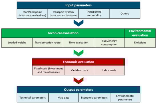
Figure 1.
Structure of sub-models for road and rail transport.
The third one, the transshipment sub-model, calculates transfers between transport modes and includes various transshipment options. It can also be used within the road or rail sub-models to calculate loading and unloading times.
The model is implemented using a combination of Python v3.13.2 and Excel. The transport system databases, fees, or toll prices are loaded from an Excel file to make them easy to edit and update. The infrastructure databases and barrier parameters (tunnel, bridge) are loaded from an Apache Parquet file which is a column-oriented data file type with an efficient size and more difficult editing options, which guarantees the integrity of the input data. The model is implemented using Jupyter Notebook v8.6.3 with significant use of the Pandas library. The main outputs of the model are exported into an Excel file where further analysis can be carried over. Each sub-model incorporates over 100 input parameters, covering specific legislative conditions, timing of specific actions, and economic aspects. The data used in the models were obtained from real measurements, expert consultations, and extensive research of publicly available data and the scientific literature. Relevant data sources are cited in the following sections.
3.1. Database of Transport Systems
Defining the transport system is an important part of the evaluation. The model contains a comprehensive database covering various transport system elements for both road and rail transport, with key types listed in Table 3 (road) and Table 4 (rail). Intermodal containers, including multiple types of ISO containers, Abroll container transport system (ACTS) containers, and Innofreight system containers, are applicable to both modes.
Table 3.
Transport system elements for the road transport sub-model.
Table 4.
Transport system elements for the rail transport sub-model.
These transport system elements can be combined to create transport systems according to specific cases. This enables the model to accurately evaluate the technical performance of each specific case without generalization which will subsequently be reflected in the economic evaluation. The model automatically verifies element compatibility and avoids infeasible configurations. Additionally, the database allows for easy integration of new elements without modifying the model, except in specific cases.
Each transport system element is characterized by several parameters, such as operating weight, dimensions, number and type of tires, and investment or annual service costs. Motor vehicles have also defined fuel/energy consumption based on manufacturers’ specifications or research. Locomotives in the database are detailed not only by general parameters (e.g., weight, number of axles, traction force) but also by specific traction characteristics for each traction system, essential for speed profile calculations.
For the case study, the selected road transport systems include semi-trailer trucks and intermodal semi-trailers compatible with ISO containers (MEGC, gaseous form of hydrogen), based on the review in Section 2.2. The rail transport system consists of electric locomotives and intermodal wagons, also compatible with ISO containers.
3.2. Infrastructure Network
Currently, the model includes only road and rail infrastructure data for the Czech Republic, with the option to integrate data from other countries if needed.
The road transport infrastructure used in this study is based on real infrastructure data from the Czech Office for Surveying, Mapping, and Cadastre. Since the model mainly focuses on freight transport, the complexity of the network was reduced by omitting irrelevant local roads that are impassable for heavy-duty vehicles. To optimize computational efficiency, municipalities with fewer than 1000 inhabitants were removed from the database, and multiple points of interest were added, resulting in a database of 1132 points.
The processed road network consists of 230,835 sections, each defined by 15 parameters such as length, route class, slope, and presence of tunnels or bridges (see Figure 2).
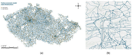
Figure 2.
(a) Road infrastructure of the model (Czech Republic); (b) road infrastructure of the model (detail at city level).
Since the road infrastructure in the model is not a replica of real-world roads, the route evaluation allows adjustments—such as defining the final section length for each route class—to improve calculation accuracy. Alternatively, users can bypass the predefined infrastructure and manually define transport routes based on length per route class.
The rail network in the model is 1:1 with the real infrastructure, excluding sidings. It consists of 2755 points and 4118 sections, each characterized by 28 parameters, including section length, maximum speed, road class, and normative length of the train, etc., see Figure 3.
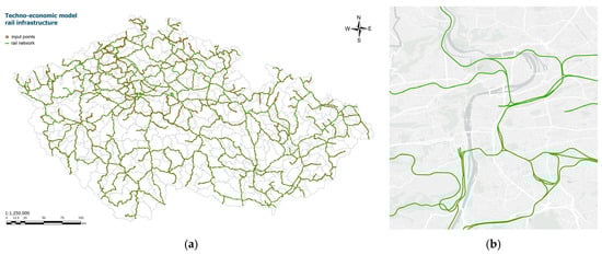
Figure 3.
(a) Rail infrastructure of model (Czech Republic); (b) rail infrastructure of model (detail at city level).
Each infrastructure section can be manually omitted, for example, in case of technical closures or other disruptions.
3.3. Technical Evaluation
The technical evaluation consists of five main steps:
- Weight calculation;
- Transport route determination;
- Fuel/energy consumption assessment;
- Total time calculation;
- Emission analysis.
As the detailed technical evaluation processes for road and rail transport are partly different, each is presented in a separate section. However, the estimation of environmental emissions applies to both transport modes and is detailed in Section 3.4.
3.3.1. Technical Evaluation of Road Transport
The first step of the technical evaluation is determining the total weight of the transport system based on the selected transport system and commodity, such as hydrogen. The weights of the transport system elements are retrieved from the database. For transported commodities, the weight can be defined in two ways:
- By density (bulk weight): The model calculates weight based on vehicle or trailer volume.
- By fixed weight per cycle: The model verifies compliance with the transport system load limits or calculates a lower loaded weight if necessary.
Once the loaded weight and total weight (Equation (1)) are determined, the load factor is calculated (Equation (2)).
where mtotal—total weight of the transport system [t]; msystem—the empty weight of the transport system [t]; mload—loaded weight [t]; melement—weight of transport system elements [t]; lf—load factor [-]; mlimit—the maximum permitted (legislative) weight for transport system [t].
The transport system is subsequently classified into the vehicle category (Table 5) considering the calculated total weight and its dimensions. The weight and height limits are subject to legislation.
Table 5.
Road transport vehicle category used in the sub-model.
The model then determines the shortest transport route that meets the defined criteria for each vehicle category (see Table 5). Dijkstra’s algorithm is used for route determination. A sample evaluation for different vehicle categories is shown in Figure 4.
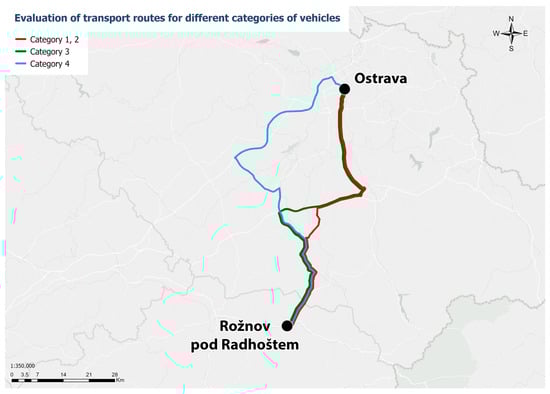
Figure 4.
Example of transport route evaluation for different vehicle categories based on weight and height.
The example demonstrates that the route with vehicles in categories 1 and 2 is the shortest (marked in red), while higher-category vehicles sometimes take longer routes along high-capacity regional roads due to vehicle weight and size limitations on local roads and streets passing through urban areas. These differences also affect the overall evaluation.
Once the transport route is determined, the model can then calculate fuel consumption. Given the complexity of theoretical consumption estimation, a simplified approach is used. Fuel consumption in this model is estimated based on the average fuel consumption defined for each motor vehicle, travel distance, and calculated load factor (Equation (2)). Fuel consumption increases with the loaded weight (higher load factor). The average consumption in the database corresponds to a load factor of 50% for each vehicle, with several adjustments made, such as the following:
- EURO VI emission standard trucks: −5 L/100 km for a load factor of 0% and +5 L/100 km for a load factor of 100%;
- Passenger cars and vans: −1.5 L/100 km for a load factor of 0% and +1.5 L/100 km for a load factor of 100%.
The fuel consumption adjustment is modeled linearly as shown in Equation (3).
where fc—theoretical fuel consumption [L/100 km]; fcaverage—average fuel consumption of motor vehicle [L/100 km]; a—constant (3 for passenger cars or vans, 10 for trucks); b—constant (1.5 for passenger cars or vans, 5 for trucks).
The total transport route may include multiple waypoints, with each section having a different load factor. This applies to both the loaded journey to the destination and the empty return trip. The total fuel consumption is then determined as shown in Equation (4).
where fctrip—trip fuel consumption [L]; fci—theoretical fuel consumption of each section [L/100 km]; si—distance of each section [km].
The final step of the technical evaluation is calculating the total transport time. The total transport time is calculated as the sum of driving time, loading, and unloading time, while also considering legislative requirements, such as the European Road Transport Agreement (AETR) limits on daily total driving time. A theoretical delay is factored in as a percentage of the total time.
Driving time is estimated based on average speeds defined for each road class and vehicle category. Since the transport route has already been determined, distances for each section are summed according to the road class. The driving time is calculated as shown in Equation (5).
where tdrive—driving time [min]; src,i—sum distance for each road class [km]; vi—average speed for each road class [km/h].
Loading and unloading times can vary depending on the transported commodity and selected transport system. For hydrogen, the filling (loading) time is considered the same as the emptying (unloading) time, as defined by Equation (6).
where tload—loading (filling) time [min]; filling rate—hydrogen filling rate [kg/min].
Once all related times are calculated, they are summed to obtain the total transport time, as shown in Equation (7).
where ttotal—total transport time [min]; tdrive—driving time [min]; tload—loading time [min]; tunload—unloading time [min]; delay—theoretical delay [%].
3.3.2. Technical Evaluation of Rail Transport
Similarly to road transport, the first step in rail transport evaluation is to calculate the total weight of the transport system (train). The calculation follows Equation (1) from Section 3.3.1. Differently, the model operates in two modes, where the loaded weight and the determined transport route are related. The first mode finds the shortest possible route (respecting train technical parameters) and determines the maximum loaded weight based on railway track parameters, particularly the lowest maximum permissible axle load. The second mode calculates the maximum loaded weight first and then determines a suitable transport route. Dijkstra’s algorithm is implemented for route determination.
Each wagon in the database has a defined maximum loaded weight for different track classes, determined by axle load limits (16 to 22.5 t/axle in the Czech Republic). The model can automatically adjust the number of wagons based on the transport route constraints (e.g., train length limits). It can handle combinations of full, empty, or partially loaded wagons, such as empty containers. The bulk weight or weight per cycle of the transported commodity is then calculated.
Since loaded weight affects route selection, other important parameters include train length, locomotive traction system, and the required minimum track curve radius. The resulting routes can be similar to the road transport examples in Figure 4 (Section 3.3.1).
Once the transport route is determined, the next step is to calculate the train’s speed profile. This involves multiple parameters such as the locomotive traction characteristics, loaded weight, track slope, various train resistance forces, etc. Due to its complexity and since it is not the main topic of the presented article, train driving dynamic calculation is not described in detail in this article; however, these sources were used for calculations of locomotive tractive effort [50], train resistances [51], braking force [52] and power, and energy calculations [53].
The core principle involves the calculation of actual speed based on the traction force of the locomotive. Speed increments are calculated for each section of the route. If a section is longer or the model identifies a longer distance of the step, the default calculation step is 100 m. Figure 5 and Figure 6 provide a sample evaluation of the speed profile and the corresponding altitude profile.
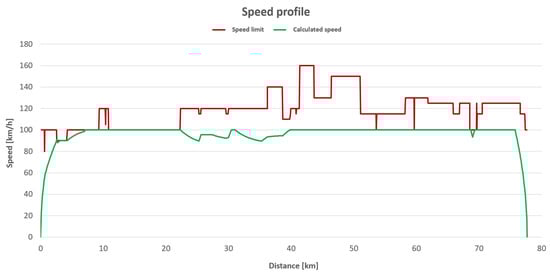
Figure 5.
Speed and altitude profile as a function of distance.
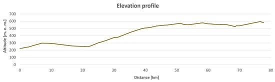
Figure 6.
Elevation profile as a function of distance.
Within each speed calculation step, forces (traction, regenerative, or braking), work, energy, and driving time are calculated in the model. A sample force diagram is provided in Figure 7.
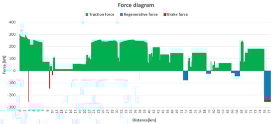
Figure 7.
Force diagram as a function of distance.
The required work is calculated based on traction or regenerative forces as shown in Equation (8).
where Wtr—work [kJ]; Fi—traction or regenerative force at section [kN]; xi—section length [m].
From the calculated work, the total traction energy consumption is calculated as in Equation (9).
where Etr—energy consumption [kWh]; η—efficiency of the locomotive [-].
The energy consumption is calculated in kilowatt-hours [kWh] for electric locomotives and liters [L] for diesel locomotives. The assumed density of diesel fuel is 0.84 kg/m3 [54], which corresponds to a diesel fuel efficiency of 10 kWh/L. The model also supports dual/hybrid locomotives.
The driving time of each section is determined within each speed calculation step, and the total driving time is obtained as a sum of the driving times of all sections, as calculated in Equation (10).
All defined times necessary to complete the task, mainly including preparing the train, loading and unloading, and various theoretical delays, are then added to the driving time to obtain the total transportation time, as shown in Equation (11).
where ttotal—total transport time [min]; tlococheck,1—locomotive preparation [min]; tload—loading time [min]; tload,delay—delay at loading [min]; ttechcheck,1—technical check of the train before drive [min]; tdrive—driving time [min]; dtcti—percentage of distance for a given track occupancy category [%]; ci—coefficient for each occupancy category [-]; ttechcheck,2—technical check of the train after drive [min]; tundload—unloading time [min]; tunload,delay—delay at unloading [min]; tlococheck,2—locomotive shutdown time (if needed) [min].
3.4. Environmental Evaluation
Reducing emissions has become a priority as transport is a significant contributor to air pollution. The developed model performs environmental evaluation when data are available. However, environmental evaluation is not considered in the presented case study. At its current stage, the model focuses solely on emissions from exhaust gases, and for electric rail transport, it uses emission factors derived from the gross electricity production set for the case of the Czech Republic. In this model, the emissions are calculated based on fuel/energy consumption (as detailed in Section 3.3.1 and Section 3.3.2) and corresponding emission factors (in [kg/L] for fuel consumption [L] and [kg/kWh] for energy consumption [kWh]), as shown in Equation (12).
where Ei—produced emission [kg]; Fc—fuel/energy consumption [L; kWh]; EFi—emission factor [kg/L; kg/kWh].
The emissions factors used in the model are sourced from the EMEP/EEA air pollutant emission inventory guidebook 2023, published by the European Environment Agency [55]. CO2 emissions are determined using combustion equations or the emission factors for a specific drivetrain. The emission factor for diesel fuel is 0.264 kg CO2/kWh (2.64 kg CO2/L). For electric rail transport, the emission factor based on gross electricity production in the Czech Republic in 2023 was 0.37 kg/kWh [4]. Other emission factors, such as the ones for SOx, NOx, and solid particles, are given in the mentioned guidebook.
3.5. Economic Evaluation
Following the detailed technical evaluation, a cost assessment is conducted. Costs are categorized into fixed and variable costs, with labor costs considered separately. The cost evaluation is based on the theoretical utilization of the transport system, which enables the percentage expression of costs to be determined relative to the time required for the evaluated transport task, for example, one cycle. This approach enables the combination of multiple transport tasks within a single transport system and facilitates cost assessment per transport task/cycle.
Fixed costs mainly include expenses related to the purchase or rental of transport systems, maintenance (annual technical inspections, regular and irregular maintenance), insurance, and road taxes (Equation (13)). Maintenance costs are defined as a fixed annual amount, assuming regular maintenance (each transportation system component in the database has predefined maintenance costs). Alternatively, maintenance costs can be evaluated based on total mileage.
where Cfix—fixed costs [EUR/cycle]; Civest—investment costs [EUR/year]; Cloan—loan repayment costs [EUR/year]; Cmaint—maintenance costs [EUR/year]; Cinsurance—insurance costs [EUR/year]; Ctax—road tax (only for road transport) [EUR/year]; TU—theoretical utilization of transport system [%].
The model also considers the lifespan of each component of the transport system. For example, a semi-trailer truck typically has a life span of approximately 6–7 years, whereas a locomotive can last around 30 years. Over the expected duration of a given project (e.g., 20 years), the company will need to replace a truck three times, while a locomotive would not require replacement, with the possibility of undergoing major modification in its mid-life. These differences across transport types are considered in the model and evaluated in all sections of the transport system.
Variable costs, as calculated in Equation (14), include road tax, tolls, and fees, tire costs based on mileage and fuel/electric energy, and operating fluid costs. Toll fees are determined based on road classification and specific toll sections. The most significant portion of variable costs comes from fuel/electric energy consumption and the use of operating fluids, such as AdBlue liquid, which are necessary to reduce diesel exhaust emissions. For rail transport, additional costs apply for the use of railway infrastructure, similar to road tolls.
where Cvar—variable costs [EUR/cycle]; Ctire—tire costs (only for road transport) [EUR/cycle]; Cfee—tolls and fees [EUR/cycle]; Cfuel—fuel/electric energy and operating fluids costs [EUR/cycle].
Labor costs are also considered in the model. The primary role is played by the crew’s wage costs, which are defined for individual positions and the number of employees. The labor costs for administrative and operational overheads are considered annually as a fixed price representing the share of company costs for these employees/departments.
where Clabour—labor costs [EUR/cycle]; Ccrew—crew wage [EUR/year]; Cadmin—administrative overhead costs [EUR/year]; Coper—operational overhead costs [EUR/year]; TU—theoretical utilization of transport system [%].
where Ctotal—total costs [EUR/cycle].
3.6. Transshipment
Transshipment between different transport modes is a crucial part of the logistics chain. It can be performed simply using handling equipment such as a container handler on a paved area, for example, near a railway station. For frequent and large-volume transfer, it is more efficient to use a stationary transfer station, which is commonly employed for handling intermodal containers.
Various types of different transshipment methods can be used within the logistics chain, each with unique technical requirements and costs. For example, transferring bulk materials using a wheel loader differs significantly in both technical specifications and costs from transferring liquid components from tanks or using a stationary transfer station for container handling.
The transshipment sub-model is significantly simpler than the sub-models for road and rail transport described above. It currently includes calculations for equipment such as wheel loaders, container handlers, and Abroll container carriers (ACTS). The technical parameters (e.g., fuel consumption, service life, loading/unloading time, and working hours) and economic parameters are defined together with other sub-models. The evaluation can be performed based on annual theoretical utilization or by assessing the manipulator’s use for a specific task. The output of this sub-model provides the annual costs or cost per ton, engine hour, cycle, or day.
4. Case Study
4.1. Selected Study Area
In this study, the southeastern region of the Czech Republic is used as a case study to validate the proposed techno-economic assessment model. Due to data limitations, accurately projecting future hydrogen demand distribution across all regions of the Czech Republic is challenging. Instead, several representative regions are selected based on population density for the case study. Figure 8 illustrates the population density and the anticipated main hydrogen pipeline network in the selected study area, which will be created through the conversion of natural gas pipelines (see Section 4.2).
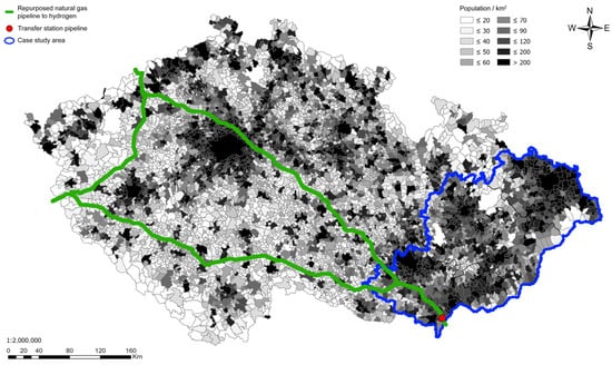
Figure 8.
Population density, converted hydrogen pipeline, and selected area for case study (marked in blue).
The study area is located in the southeastern Czech Republic, characterized by high population density and positioned outside the main hydrogen transport pipeline routes. The terrain of the selected area is predominantly flat with minor hills but lacks significant elevation differences. The area is home to about a third of the Czech Republic’s population (about 3 million people) and includes the second and third largest cities. Its eastern section includes the Ostrava Metropolitan Area (982,000 inhabitants), a historically energy-intensive industrial hub (mines, steel production) that is currently undergoing industrial transformation. One of the region’s key initiatives is the establishment of the Moravian-Silesian Hydrogen Cluster [56]. Industry in the study area is generally widespread, from heavy machinery to petrochemical and automotive. The region also has a dense public transport network, which potentially contributes to a higher demand for hydrogen in the region. The region is well connected by a main electrified railway line, which is part of the TEN-T network, offering the potential for multimodal transport solutions. The evaluated region extends within a 50 km radius of the railway line, as shown in Figure 9. Figure 9 highlights the infrastructure network of the selected area, focusing on electrified railway lines and primary road networks while excluding third-class and lower-rate routes. However, the model incorporates all infrastructure for evaluations.
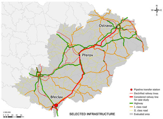
Figure 9.
Selected road and rail infrastructure of the study area.
The study area is divided into smaller sections based on administrative districts of municipalities with extended jurisdiction (microregions). The transportation costs are calculated for each municipality with extended jurisdiction, with variations for other municipalities within the microregion differing by only a few percent.
The main hydrogen logistics hub is proposed near the town of Břeclav (25,000 inhabitants), close to the border with Austria and Slovakia. Today, the site serves as an extensive natural gas compressor and transfer station within the pipeline network, offering the opportunity to develop key hydrogen infrastructure here, such as filling stations, handling facilities, and storage areas. The proposed logistics hub (compressor station) is situated 3 km from the highway, with the nearest railway station 5 km away. While the railway track passes only 400 m away from the hub, it would be possible to construct a railway siding to the logistics hub to streamline the rail transport logistics. However, this option is excluded from the case study due to the high investment costs required for railway infrastructure. The situation overview is shown in Figure 10.
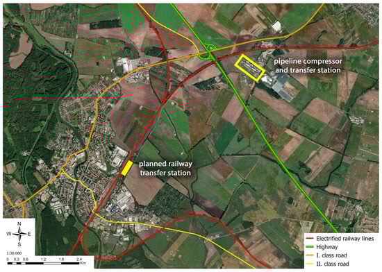
Figure 10.
Situation overview of the Břeclav area with the pipeline transfer station, railway station, and transport infrastructure.
4.2. Strategies in Hydrogen Transportation
Legislation and government policies are significant aspects in the techno-economic assessment of hydrogen logistics. According to the Hydrogen Strategy of the Czech Republic [34], the country does not anticipate significant hydrogen imports by 2030. Instead, local production will be the primary source, utilizing electrolysers and, to a lesser extent, pyrolysis. The hydrogen production will rely on renewable energy sources such as wind, solar, and hydropower, along with surplus nuclear energy. In the strategic planning, the hydrogen production will be concentrated in “local islands” near areas with high hydrogen demand. The anticipated hydrogen demand in the Czech Republic is 129,000 t in 2030, increasing up to 385,000 t for the low scenario, respectively, and up to 1,322,000 t for the high scenario, in 2040 [34]. The projection then assumes a demand of 1,160,000 t in 2050 for the low scenario, or 1,835,000 t for the high scenario [34]. The projection is only for the whole country and does not specify demand by region which this case study would benefit from.
After 2030, hydrogen imports are expected to increase substantially, offering lower costs compared to domestic production. Local production would face limitations due to the country’s geographic conditions, which might restrict the potential for utilizing renewable energy sources. Compared to Germany, North Africa, Baltic Sea states, or Ukraine, solar and wind energy production in the Czech Republic is less efficient despite similar investment costs and installed capacities [4]. To facilitate future hydrogen import, NET4GAS, the operator of the Czech gas network, is planning to convert portions of its natural gas pipelines to hydrogen by 2030, as shown in Figure 11 [57].
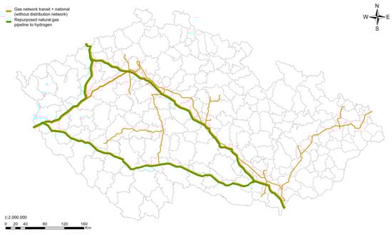
Figure 11.
Map of considered conversion of natural gas pipeline to hydrogen pipeline; based on NET4GAS plan [57].
4.3. Hydrogen Logistic Chain
The case study focuses on two major transportation methods, i.e., purely road transport (Option 1) and multimodal transport including road and rail (Option 2). Figure 12 illustrates the logistics chain of road and multimodal transport, which is simulated and assessed in this study.
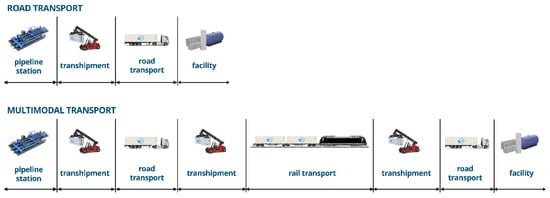
Figure 12.
Logistics chain of road and multimodal transport.
In order to compare the techno-economic performance of the two options, the same transport unit, with pressure cylinders placed in an ISO container (MEGC), is used for both road and rail transport. It is designed for gaseous hydrogen at a pressure of 380 bars and has a transported capacity of 1029 kg per ISO container (unit), as detailed in Table 1 (Section 2.2.1). The ISO container can be used for standardized road container semi-trailers and railway cars. For all transshipments, a regular container handler will be used. The container handling time (loading or unloading) was assumed to be 3 min and was obtained from consultation with experts based on the conditions of the considered intermodal terminals. For comparison, a study [58] states a time of 1 min 45 s for unloading a 40 ft container and 2 min for loading. Delays are also considered within the individual models, e.g., in the case of rail transport, it takes 15 min for loading and unloading, see Equation (11) and Table A2.
The container-filling process is not included in the assessment. The system boundary of the assessment starts from the container loading process. For road transport, the vehicle will go directly to the destination. For multimodal transport, the vehicle will first go to the railway station (Břeclav) where the container is transshipped to the railway wagon. In this study, 20 Sggrs wagons (intermodal container wagons) are considered for rail transport. Once loaded, the train will go to the regional intermodal hub—Přerov or Ostrava (see Figure 10). The selection of these intermodal hubs was based on their existing role as large marshaling yards, equipped with numerous transshipment options and amenities, supporting their significance in the region. It is assumed that these intermodal hubs will also serve as regional hydrogen transshipment points in the future, thanks to their connections to important roads (and railways). The containers will be transshipped using container handlers from railway wagons to road trailers and then transported to the destination.
The logistics chain was evaluated as continuous, with each step seamlessly following the next without any downtime, which is favorable for rail transport. The transport of energy commodities can be considered a priority freight train, which, in certain cases, takes precedence over passenger transport.
For both Option 1 and Option 2, it is assumed that the cylinder containers will be emptied, and the hydrogen will be compressed/pumped into stationary storage vessels at the customer’s premises. During this process, the container will remain on the road trailer for an extended period, leading to additional waiting time. Once emptied, the cylinders will be transferred back to the logistics hub. Removing the container from the trailer at the customer’s site would require additional container handling equipment and time. Given the high cost of handling equipment, this option will increase the cost of emptying the container and the total transportation costs.
The time required to empty the containers and the corresponding flow rate are crucial factors in hydrogen logistics. However, most of the existing studies focus on fuel cell vehicle filling stations, and a maximum discharging rate of 7.2 kg/min was reported [59,60]. A study by Eißler et al. [61] measured a gaseous hydrogen flow rate of 12.2 kg/min when discharging from a 500 bar trailer to a 200 bar stationary storage tank. In this study, a mid-range value of 10 kg/min is used in the calculations.
4.4. Techno-Economic Assessment
The case study aims to determine the theoretical transport costs per unit weight of hydrogen (EUR/t of hydrogen) for each served microregion and to compare the techno-economic performances of road transport versus multimodal transport incorporating railways.
The model incorporates more than 100 technical and economic parameters. Due to space limits, only a selection of key input parameters is presented in Table 6. The full list of input parameters for each sub-model is provided in Table A1, Table A2 and Table A3 in Appendix A.
Table 6.
Selected input parameters.
The average fuel consumption for a semi-trailer tractor, as a parameter that can affect the resulting costs, depends on the specifically selected type and its engine. The fuel consumption of the type considered in the given case study was derived from technical parameters and operating experience and is similar to the given EURO VI-E vehicle category.
Note that all results are obtained based on the theoretical utilization (by time) of each vehicle. The total time for one cycle is determined and divided by the annual working time, which is calculated with the daily working hours and annual working days. It is assumed that each vehicle is also assigned to other tasks throughout the year (remaining annual utilization); for example, a truck might be used for further transport, or a container handler used for other activities within the logistics hub. The individual steps in the logistic chain follow one another without downtime.
In terms of cost, the presented results include only the cost of transporting to microregions’ centers without the costs of intermodal units (i.e., containers) due to the lack of available data on container prices, maintenance costs, and hydrogen demand in the selected area. The results account for fixed costs associated with trucks and trains, such as investment costs, maintenance costs, labor costs, and operating costs, primarily fuel/energy expenses, tires, tolls, and other related expenditures. All calculated costs are based on 2024 price levels.
4.4.1. Option 1—Road Transport
Option 1 considers only road transport, utilizing a single logistics hub located directly at the pipeline transfer station in Břeclav. The evaluation was carried out using the proposed techno-economic model while adhering to the logistics chain in Figure 12. The results are presented in geographic form using the QGIS v3.30 software, as shown in Figure 13.
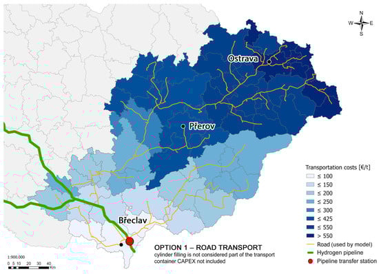
Figure 13.
Transportation costs for the evaluated area—road transport.
Transportation costs increase with distance. For short distances, costs are estimated at around 55 EUR/t for up to 10 km and 100 EUR/t for distances up to 30 km. For distances around 100 km, the transportation costs rise to approximately 220 EUR/t. The longest distance in the evaluated area is 256 km with a transportation cost of 607 EUR/t. Notably, the Ostrava metropolitan area, where significant demand for hydrogen is anticipated, is estimated to have a high transportation cost ranging from 425 to 600 EUR/t. The average transportation cost across the evaluated area is 348 EUR/t.
In this study, a cylinder dispense rate of 10 kg/min was assumed, meaning it would take approximately 100 min to empty a full container. Based on a theoretical time utilization of the transport system, the calculated cost per transport system is 32 EUR/t for 100 min of container emptying. Despite covering these costs, it is still a more cost-effective option than container trailers with side unloading, which are more expensive and heavier, with a higher operating cost. Using a container handler at each destination is an even more expensive alternative. Therefore, leaving the container on the trailer during the emptying process is considered the most economical option.
4.4.2. Option 2—Multimodal Transport
The second option for establishing a logistics chain involves multimodal transport utilizing railways, and the model results are presented in Figure 14. In Option 2, the same containers as in Option 1 (MEGC) are used. Multimodal transport requires multiple intermodal terminals to effectively serve the region. Two intermodal terminals, Přerov and Ostrava, are selected for this study, and both terminals are equipped with container handlers. Their distribution areas were defined by a radius of 50 km from each terminal, considering the shortest possible road transport distance. The area around Břeclav (pipeline transfer station) will continue to be served exclusively by road transport with the same cost as in Option 1.
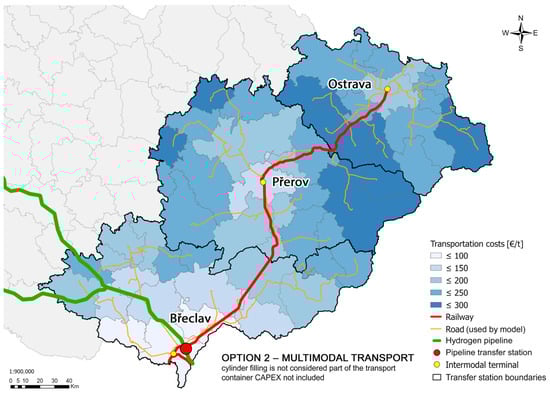
Figure 14.
Transportation costs for the evaluated area—multimodal transport.
While it is possible to use more terminals with smaller distribution areas within the region, doing so would require building new facilities and purchasing container handlers, which could significantly increase the overall costs of the logistics chain.
Compared to road transport (Figure 13), the transportation costs of multimodal transport (Figure 14) reveal a significant reduction in costs in more remote areas and a more even cost distribution. The lowest costs of Option 2 remain the same as those of Option 1 (road transport), as the area nearest to the pipeline transfer station is served without rail transport. The microregions served by the intermodal terminal in Přerov have the lower average costs of 214 EUR/t (down from 339 EUR/t in Option 1), representing a 37% decrease. The microregions served by the intermodal terminal in Ostrava have lower average costs, dropping to 244 EUR/t (from 541 EUR/t in Option 1) with a 55% reduction. The highest cost in the evaluated area is reduced to 292 EUR/t in Option 2, and the average transportation cost is 205 EUR/t.
5. Discussion
As the models use a real infrastructure network, higher-class routes such as highways, first-class roads, etc., are preferred in freight transport evaluation. This preference can lead to differences in areas that have the same direct distance from the starting point. In reality, however, the actual route may involve significant differences in distance or toll payment, which can ultimately result in varying transportation costs. An example from the case study is presented in Table 7.
Table 7.
Example of the transport costs for microregions with similar direct distances.
In the transport model, the journey to the destination with loaded containers and the return journey with empty containers are considered. Since the weight of the transported hydrogen in a single container is only about 1 ton, and the primary weight being transported is the container itself, the differences in operating costs for the journey to the destination and the return journey are not significant, though they are not negligible.
It is necessary to point out again that the presented results include only the investment costs of the semi-trailer tractor and semi-trailer, respectively, and the costs of locomotives and railcars. The costs of containers were not included due to the lack of available data on container prices, maintenance costs, and, mainly, hydrogen demand in the selected area, which is necessary to evaluate the number of containers needed to cover the area by multimodal transport. The results presented, therefore, include purely transportation costs. This method, on the other hand, brings the possibility of using the case study results and simply adding them to the evaluated costs for different numbers of containers based on the hydrogen demand in the area.
5.1. Comparison Option 1 vs. Option 2
The breakdown of the transportation cost of Option 1 and Option 2 is compared and presented in Table 8.
Table 8.
Comparison of the transportation costs between Option 1 and Option 2.
As previously mentioned, the lowest cost (51 EUR/t) remains the same for both options since the area around Břeclav is served exclusively by road transport in both cases.
However, multimodal transport proves to be significantly more cost-effective than road transport, especially in the Ostrava distribution area. The rail segment in multimodal transport benefits from lower unit transportation costs thanks to its high capacity, and the intermodal terminals help to shorten road transport distances and further lower the cost. In Option 1 (road transport only), the average road transport distance is 141 km, while in Option 2 (multimodal transport), it decreases to just 47 km. The longest road distance is reduced from 256 km (Option 1) to 126 km (Option 2). Additionally, the municipality with the highest transportation costs in Option 1 (607 EUR/t) sees a considerable reduction to 292 EUR/t in Option 2.
Since many parameters can be volatile, a sensitivity analysis of the most influential ones was performed. In general, these are mainly variable costs, such as fuel or electricity prices, or labor costs. Most other costs increase steadily, aligned with inflation.
In the case of fuel price, the analysis was performed for an increase/decrease of 20%. It turned out that with a 20% increase in fuel prices, operating costs increased by an average of 9.8%, respectively, and decreased by 9.5% for a 20% decrease in fuel price. It was also interesting to note that for shorter distances, the increase/decrease was higher, around 13–15%, but for longer distances, it was only around 8%, which was caused by a greater share of toll costs related to the higher use of toll roads. However, the impact of volatile fuel prices on total costs is relatively small, only around 5%. For rail transport, the change of 20% in electricity price affects variable costs by 9.5% and total costs by 5.5%, comparable to the change in fuel price for road transport.
A 20% increase in the purchase cost will only translate into a 2.4% increase in total costs, both for road and rail transport systems. A 20% increase in labor costs will lead to a 5.1% increase in total costs.
The case study evaluated only one technology (MEGC, 380 bar). It is important to emphasize that the use of different technology can affect the entire logistics chain and the resulting costs, where for example, implementing multimodal transport may be more complicated and not bring as significant benefits.
5.2. Contributions, Limitations, and Future Works
5.2.1. Contributions
The proposed techno-economic assessment (TEA) model addresses areas that were not fully explored in previous research, such as integrating real infrastructure into the model and performing detailed calculations of theoretical energy consumption—particularly for rail transport. This approach also enables a more precise estimation of environmental emissions.
The model was demonstrated with a case study in the southeastern region of the Czech Republic. This region includes both densely populated areas and the Ostrava metropolitan area, which is currently undergoing industrial transformation. The case study compared road transport with multimodal transport (road and rail).
The model is designed as a general framework, so it can be applied to various types of roads and rail transport without major modifications. The same applies to hydrogen transport options, where individual technologies are undergoing rapid development. The model already incorporates the findings of extensive research, and it is assumed, thanks to the model’s comprehensive structure, that only minor changes will be necessary, such as adding new transport system elements to the database or changing hydrogen filling parameters. In the event of entirely new and distinct technology, the model will undoubtedly require adjustments. Nevertheless, the fundamental evaluations will remain consistent.
The model can be integrated into optimization tools. While it can be used directly for a highly detailed analysis, this increases the computational requirements, which is not desirable in most cases. Otherwise, the model can be simplified by fixing certain parameters and allowing only selected variables to change, effectively simplifying the model to one equation.
Additionally, the model can support both pre-processing and post-processing tasks. A typical approach includes the following:
- Pre-calculations using the TEA model (e.g., calculating costs and travel time for all routes) as inputs for an optimization tool;
- Optimization processing (e.g., determining optimal transfer station locations and supply routes);
- Refining the optimization results with the use of the TEA model for more precise cost and time estimations.
The previous version of the presented model was used for pre-calculations in [62,63,64].
5.2.2. Limitations and Future Works
One of the main difficulties of the presented model is obtaining real and verified data, particularly regarding container prices and maintenance costs. Manufacturers do not publicly disclose pricing for individual solutions, and the limited data are available in only two scientific publications. Additionally, rapid development in the field further complicates data collection. However, acquiring this information is essential for accurate planning and evaluation, ultimately enabling the assessment of different hydrogen transportation methods. The same issue applies to hydrogen demand, which is crucial for determining the number of containers needed, but remains unknown for the selected area.
Certain transportation time delays are considered in both Options 1 and 2 during the modeling and assessment process. Despite this, Option 2 demonstrated better performance in most of the parameters due to the optimal use of railway transport. The logistics chain was assessed as continuous, with each step following seamlessly without downtime. While this is generally feasible for road transport, it presents a challenge for rail transport. Rail operations rely on timetables set up a year in advance, and passenger transport is generally considered a significant priority. As a result, freight transport often experiences delays, waiting for free track capacity, running mainly at night, and making multiple stops along the route. A loaded train can sometimes be held for several hours before departure, leading to increased transportation costs due to higher train utilization. Accurately estimating these delays in advance is difficult, as they depend on the specific transport routes, the priority of the train, and the carrier’s technical capabilities. The presented model already addresses timetable constraints by utilizing delay coefficients (see Equation (11)) based on the analysis of historical timetables. These coefficients reflect the need to stop due to passenger transport priority, delays at departures, etc. This key parameter will be further analyzed and refined in follow-up research, with planned collaboration with a major freight carrier and the infrastructure operator responsible for timetable planning.
Intermodal terminals can connect different transport modes and be used for various tasks, lowering transshipment costs. In the presented case study, their location was selected manually based on multiple criteria, primarily their current role and infrastructure options. Future research is aimed at the country level, so it is more complex to specify the terminals’ locations. The optimization tools will be used, incorporating real-world data and conditions to determine the most effective terminal locations.
The development of hydrogen strategic support is changing quickly. It can be expected that, due to the support of a zero-emission economy, the EU, and, therefore, individual states, will create subsidy titles to support the implementation of hydrogen. For this reason, the initial higher costs of hydrogen transport compared to already established mass commodities such as natural gas or fossil fuels can be mitigated by subsidies. Technological development can also be expected in the future, which will probably lead to lower costs for individual technologies. For example, the price of the MEGC system is currently high, see Section 2.2.1, but its gradual decrease can be expected.
Environmental evaluation was not performed in this case study. To perform it adequately, it is necessary to analyze a number of different parameters and influences. It would also be necessary to cover the influence of individual vehicle types and their drivers, mainly semi-trailer tractors and container handlers. The potential of using hydrogen as fuel for vehicles in a given logistics chain is also promising. Future work should aim to cover environmental parameters in more detail.
6. Conclusions
This study begins with a literature review to summarize the current state of hydrogen distribution. Most existing studies focus more on long-distance hydrogen transport, while medium- and short-distance transports are underexplored, and rail transport is rarely mentioned. Based on the literature review and an analysis of existing challenges, this study develops a model to evaluate the technical, economic, and environmental performance of the hydrogen logistic chain. Finally, the proposed model is demonstrated through a case study conducted in selected regions in the southern Czech Republic.
The main conclusions of this study include the following:
- Multimodal transport significantly reduces transportation costs compared to road transport. The highest transportation costs are reduced by 52%, and the average transportation costs are reduced by 41%.
- Integrating real infrastructure into the model leads to variations in transportation costs for similar distances due to differences in variable costs (mainly tolls).
- A comprehensive evaluation of all key components of the logistics chain is essential for an accurate TEA.
- Acquiring real and verified data is crucial but remains one of the most challenging aspects.
This study serves as the first attempt to develop a techno-economic assessment model for evaluating the domestic hydrogen logistic chain. In addition, as the case study covered a relatively large area of the Czech Republic and is based on real infrastructure and data, the findings provide valuable insights for future hydrogen deployment and strategic planning in the country.
Author Contributions
Conceptualization, D.P. and M.P.; methodology, D.P.; software, D.P.; validation, M.P., X.J. and P.S.; formal analysis, D.P.; investigation, D.P.; resources, M.P. and P.S.; data curation, D.P.; writing—original draft preparation, D.P. and X.J.; writing—review and editing, D.P., X.J. and M.P.; visualization, D.P.; supervision, M.P. and P.S.; project administration, M.P.; funding acquisition, M.P. All authors have read and agreed to the published version of the manuscript.
Funding
This work was supported by the project “Lifecycle of New Energy Sources”, funded as project No. CZ.02.01.01/00/23_020/0008508 by Programme Johannes Amos Comenius, call Intersectoral cooperation.
Data Availability Statement
The processed data presented in this study are listed within the article and the Appendix. The raw data supporting the conclusions of this article will be made available by the authors on request.
Conflicts of Interest
The authors declare no conflicts of interest. The funders had no role in the design of the study; in the collection, analyses, or interpretation of data; in the writing of the manuscript; or in the decision to publish the results.
Abbreviations
The following abbreviations are used in this manuscript:
| ACTS | Abroll container transport system |
| AETR | Accord européen sûr les transports routiers (European Road Transport Agreement) |
| Eh | Engine hour |
| EU | European Union |
| EUR | Euro (currency) |
| ISO | International Organization for Standardization |
| LCA | Life cycle assessment |
| LOHC | Liquid Organic Hydrogen Carriers |
| MEGC | Multi-element Gas Container |
| TEA | Techno-economic assessment |
Appendix A
Table A1.
List of all input parameters—road transport sub-model.
Table A1.
List of all input parameters—road transport sub-model.
| Parameter | Value | Unit |
|---|---|---|
| AdBlue consumption | 2 | L/100 km |
| AdBlue price | 1.4 | EUR/L |
| Administrative overhead costs | 7500 | EUR/year |
| Allowed combinations of transportation system elements | [‘0000’, ‘1000’, ‘2000’, ‘3000’, ‘0500’, ‘1500’, ‘2100’, ‘2200’, ‘2300’, ‘2210’, ‘3010’, ‘3001’, ‘3400’, ‘3410’, ‘3401’] | |
| Average speeds | pd.DataFrame ({‘tridaSilnice’: [‘dalnice’, ‘silniceItridy’, ‘silniceIItridy’, ‘silniceIIItridy’, ‘mesto’, ‘ostani’], ‘kat_00’: [125, 80, 80, 60, 35, 20], ‘kat_01-02’: [115, 80, 80, 60, 35, 15], ‘kat_03-04’: [80, 65, 60, 30, 30, 10]}) | km/h |
| Container—definition (name) | Hexagon Purus Type 4 H2 380 bar (1029 kg H2) 40 ft | |
| Container—empty weight | 18,971 | kg |
| Container—length | 12,116 | mm |
| Container—lifespan | 30 | year |
| Container—price | 220,000 | EUR |
| Container—regular maintenance | 2000 | EUR/year |
| Container—volume | 39.9 | m3 |
| Delay on the journey | 10 | % |
| Destination point | variable | |
| Diesel fuel price | 1.6 | EUR/L |
| Driver wage costs | 2000 | EUR/month |
| Emission class fee | 0 | EUR/year |
| Hydrogen filling/emptying time | 10 | kg/min |
| Interest rate for the loan | 7 | % |
| Interest rate for own resources | 10 | % |
| Loan maturity | 5 | year |
| Motor oil price | 8 | EUR/L |
| Motor vehicle—ad hoc maintenance expenses | 2000 | EUR/year |
| Motor vehicle—average fuel consumption (load factor 50%) | 23 | L/100 km |
| Motor vehicle—category | 2 | |
| Motor vehicle—definition (name) | Volvo FH 16 4x2 | |
| Motor vehicle—emission category | N3 | |
| Motor vehicle—emission class | EURO VI | |
| Motor vehicle—empty weight | 7130 | kg |
| Motor vehicle—insurance | 1000 | EUR/year |
| Motor vehicle—maximum load | 18,000 | kg |
| Motor vehicle—maximum permissible weight | [{‘pocetNaprav’: 2, ‘limitHmotnost’: 18}, {‘pocetNaprav’: 3, ‘limitHmotnost’: 26}, {‘pocetNaprav’: 4, ‘limitHmotnost’: 32}] | t |
| Motor vehicle—MOT + emissions costs | 170 | EUR/year |
| Motor vehicle—number of axles | 2 | |
| Motor vehicle—number of tires | 6 | |
| Motor vehicle—price | 140,000 | EUR |
| Motor vehicle—price of tires | 640 | EUR |
| Motor vehicle—regular maintenance | 6000 | EUR/year |
| Motor vehicle—tire type | 315/70 R22.5 | |
| Motor vehicle (rigid chassis)—lifespan | 6 | year |
| Motor vehicle (semi-trailer)—lifespan | 5 | year |
| Multimodal system type | ISO container | |
| Number of containers per transport system | 1 | |
| Number of shifts per day (2 drivers) | 2 | |
| Operating overhead costs | 7500 | EUR/year |
| Own resources at the beginning | 160,000 | EUR |
| Project length | 10 | year |
| Required payback | 5 | year |
| Road tax for trailers with a maximum permissible weight of over 12 t | 144 | EUR |
| Starting point | variable | |
| Tires—lifespan | 120,000 | km |
| Trailer—ad hoc maintenance expenses | 800 | EUR/year |
| Trailer—category | 1 | |
| Trailer—definition (name) | Koegel Port 45 Triplex container trailer | |
| Trailer—empty weight | 4480 | kg |
| Trailer—height | 1100 | mm |
| Trailer—insurance | 800 | EUR/year |
| Trailer—length | 12,200 | mm |
| Trailer—lifespan | 10 | year |
| Trailer—max axle load | 9000 | kg |
| Trailer—maximum load | 39,000 | kg |
| Trailer—maximum permissible weight | [{‘pocetNaprav’: 2, ‘limitHmotnost’: 18}, {‘pocetNaprav’: 3, ‘limitHmotnost’: 24}, {‘pocetNaprav’: 4, ‘limitHmotnost’: 32}] | t |
| Trailer—MOT + emissions costs | 59.2 | EUR/year |
| Trailer—number of axles | 3 | |
| Trailer—number of tires | 6 | |
| Trailer—price | 36,000 | EUR |
| Trailer—price of tires | 560 | EUR |
| Trailer—regular maintenance | 1000 | EUR/year |
| Trailer—tire type | 385/65 R22.5 | |
| Trailer—volume | 39.9 | m3 |
| Transport system—maximum permissible weight | 48 | t |
| Weight per container | 1029 | kg |
| Working days of the week | 7 | |
| Working shift length | 9 | h |
| Working weeks of the year | 52 | |
| Year-on-year increase in expenses | 3 | % |
| Year-on-year increase in investments | 1 | % |
| Year-on-year revenue growth | 3.5 | % |
| Year-on-year wage increase | 4.5 | % |
Table A2.
List of all input parameters—rail transport sub-model.
Table A2.
List of all input parameters—rail transport sub-model.
| Parameter | Value | Unit |
|---|---|---|
| Administrative overhead costs | 6000 | EUR/year |
| Allocated code for combined transport | not specified | |
| Annual theoretical route composition—standard | 90 | % |
| Braking acceleration | 0.2 | m/s |
| Container—definition (name) | Hexagon Purus Type 4 H2 380 bar (1029 kg H2) 40 ft | |
| Container—empty weight | 18,971 | kg |
| Container—general repair | 15 | year |
| Container—general repair price | 20,000 | EUR |
| Container—length | 12,116 | mm |
| Container—lifespan | 30 | year |
| Container—price | 220,000 | EUR |
| Container—volume | 39.9 | m3 |
| Container loading time | 3 | min |
| Container unloading time | 3 | min |
| Crew at the station costs | 44,000 | EUR/year |
| Crew salary | 22,000 | EUR/year |
| Delay in loading | 15 | min |
| Delay in unloading | 15 | min |
| Delay coefficient—track occupancy category 100% | 0.3 | |
| Delay coefficient—track occupancy category 38% | 0 | |
| Delay coefficient—track occupancy category 67% | 0.05 | |
| Delay coefficient—track occupancy category 77% | 0.1 | |
| Delay coefficient—track occupancy category 84% | 0.15 | |
| Delay coefficient—track occupancy category 92% | 0.22 | |
| Destination point | variable | |
| Diesel fuel price | 1.6 | EUR/L |
| Dispatching costs | 120,000 | EUR/year |
| Emission allowance price | 67.33 | EUR/t CO2 |
| Interest rate for the loan | 7 | % |
| Interest rate for own resources | 10 | % |
| The iterative step of calculating train driving dynamics | 0.1 | km |
| Loan maturity | 10 | year |
| Locomotive—continuous traction force | 250 | kN |
| Locomotive—continuous traction power on the AC 15 kV system | 6400 | kW |
| Locomotive—continuous traction power on the AC 25 kV system | 6400 | kW |
| Locomotive—continuous traction power on the DC 1.5 kV system | 3500 | kW |
| Locomotive—continuous traction power on the DC 3 kV system | 6000 | kW |
| Locomotive—definition (name) | Siemens Vectron MS | |
| Locomotive—efficiency AC system | 0.85 | % |
| Locomotive—efficiency DC system | 0.8 | % |
| Locomotive—general repair | 15 | year |
| Locomotive—general repair price | 1,640,000 | EUR |
| Locomotive—length | 18,980 | mm |
| Locomotive—lifespan | 30 | year |
| Locomotive—maximum force of the electrodynamic brake | 240 | kN |
| Locomotive—maximum speed | 160 | km/h |
| Locomotive—maximum traction force | 300 | kN |
| Locomotive—maximum traction power on the AC 15 kV system | 6400 | kW |
| Locomotive—maximum traction power on the AC 25 kV system | 6400 | kW |
| Locomotive—maximum traction power on the DC 1.5 kV system | 3500 | kW |
| Locomotive—maximum traction power on the DC 3 kV system | 6000 | kW |
| Locomotive—minimum track load class | C2 | |
| Locomotive—price | 4,080,000 | EUR |
| Locomotive—regular maintenance | 140,000 | EUR/year |
| Locomotive—traction type | electrified | |
| Locomotive—weight | 87 | t |
| Locomotive—wheel arrangement | Bo’ Bo’ | |
| Locomotive preparation time | 20 | min |
| Locomotive shutdown time | 20 | min |
| Max train speed | 100 | km/h |
| Multimodal system type | ISO container | |
| Percentage of canceled transport trips per year | 5 | % |
| Number of crew per system | 4 | |
| Number of locomotives—pull | 1 | |
| Number of locomotives—push | 0 | |
| Number of shifts per day | 2 | |
| Number of train drivers per system | 4 | |
| Number of wagons | 16 | |
| Operating overhead costs | 6000 | EUR/year |
| Own resources at the beginning | 800,000 | EUR |
| Product factor | P2—nákladní doprava nespecifická | |
| Project length | 30 | year |
| Renewable energy fee | 19.8 | EUR/MWh |
| Required payback | 10 | year |
| Sggrs wagon load limits for each track load class | [{“A1”, 67.1; “B1”, 79.1; “B2”, 79.1; “C2”, 94.1; “C3”, 94.1; “C4”, 94.1; “D2”, 106.1; “D3”, 106.1; “D4”, 106.1}] | |
| Správa železnic—basic price per unit of transport performance (coefficient ZI) | 0.0029224 | EUR/tkm |
| Správa železnic—basic price per unit of transport performance (coefficient ZRP) | 0 | EUR/tkm |
| Správa železnic—the coefficient of locomotive is equipped with ETCS | 0.9 | |
| Správa železnic—product factor coefficient P1 | 1 | |
| Správa železnic—product factor coefficient P2 | 0.85 | |
| Správa železnic—product factor coefficient P3 | 0.2 | |
| Správa železnic—product factor coefficient P4 | 0.55 | |
| Správa železnic—product factor coefficient P5 | 2 | |
| Starting point | variable | |
| Time of direction change at the dead-end track | 15 | min |
| Time of connection during manipulation | 8 | min |
| Time of stop on the track during the drive | 10 | min |
| Time of the technical check of the train after driving | 10 | min |
| Time of the technical check of the train before driving | 60 | min |
| Track load class | [{1, “A1”, 16; 2, “B1”, 18; 3, “B2”, 18; 4, “C2”, 20; 5, “C3”, 20; 6, “C4”, 20; 7, “D2”, 22.5; 8, “D3”, 22.5; 9, “D4”, 22.5}] | |
| Traction electricity price | 111.5 | EUR/MWh |
| Traction characteristic—Siemens Vectron above critical speed | P/(v/3.6) | |
| Traction characteristic—Siemens Vectron below critical speed | −0.3529 × v + 300 | |
| Train driver salary | 36,000 | EUR/year |
| Wagon—general repair | 15 | year |
| Wagon—general repair price | 56,000 | EUR |
| Wagon—length | 26,700 | mm |
| Wagon—length of the loading area | 24,750 | mm |
| Wagon—lifespan | 30 | year |
| Wagon—number of axles | 6 | |
| Wagon—price | 116,000 | EUR |
| Wagon—regular maintenance | 10,400 | EUR/year |
| Wagon—technical normative | T4—ložené čtyřnápravové nákladní vozy | |
| Wagon—type | Sggrs | |
| Wagon—weight | 28,900 | kg |
| Wagon with reduced noise emissions | Ano | |
| Weight per container | 1029 | kg |
| Working days of the week | 7 | |
| Working shift length | 12 | h |
| Working weeks of the year | 52 | |
| Year-on-year increase in expenses | 3 | % |
| Year-on-year increase in investments | 1 | % |
| Year-on-year revenue growth | 3.5 | % |
| Year-on-year wage increase | 4.5 | % |
Table A3.
List of all input parameters—transshipment sub-model.
Table A3.
List of all input parameters—transshipment sub-model.
| Parameter | Value | Unit |
|---|---|---|
| Container manipulation time—attachment | 0.5 | min |
| Container manipulation time—detachment | 0.5 | min |
| Container manipulation time—transfer 1 | 1 | min |
| Container manipulation time—transfer 2 | 1 | min |
| Container manipulator—average fuel consumption | 16 | L/Eh |
| Container manipulator—lifespan | 20 | year |
| Container manipulator—price | 400,000 | EUR |
| Container manipulator—regular maintenance | 12,000 | EUR/year |
| Driver wage costs | 1310 | EUR/month |
| Fuel price | 1.6 | EUR/L |
| Number of shifts per day | 1 | |
| Working days of the week | 7 | |
| Working shift length | 12 | h |
| Working weeks of the year | 52 |
References
- Fuels—Higher and Lower Calorific Values. Online. The Engineering ToolBox. 2025. Available online: https://www.engineeringtoolbox.com/fuels-higher-calorific-values-d_169.html (accessed on 19 January 2025).
- Communication from the Commission to the European Parliament, the Council, the European Economic and Social Committee and the Committee of the Regions: A Hydrogen Strategy for a Climate-Neutral Europe; European Commission: Brussels, Belgium, 2020; p. 24. Available online: https://eur-lex.europa.eu/legal-content/EN/TXT/PDF/?uri=CELEX:52020DC0301 (accessed on 22 October 2024).
- Global Hydrogen Review 2024; International Energy Agency: Paris, France, 2024; p. 295. Available online: https://iea.blob.core.windows.net/assets/89c1e382-dc59-46ca-aa47-9f7d41531ab5/GlobalHydrogenReview2024.pdf (accessed on 22 October 2024).
- Vodíková Strategie České Republiky: Aktualizace 2024; s. 128; Ministry of Industry and Trade of the Czech Republic: Praha, Czech Republic, 2024. Available online: https://mpo.gov.cz/assets/cz/prumysl/strategicke-projekty/2024/7/Vodikova-strategie-CR-aktualizace-2024.pdf (accessed on 3 November 2024). (In Czech)
- Vodíková Mapa ČR|Centrum dopravního výzkumu, v. v. i. Available online: https://www.cistadoprava.cz/mapy/h2/ (accessed on 4 November 2024). (In Czech).
- Poul, D.; Gregor, J.; Pavlas, M.; Van Fan, Y. Techno-economic model of multimodal transport. In 6th International Conference on Technologies & Business Models for Circular Economy: Conference Proceedings; University of Maribor Press: Maribor, Slovenia, 2024; p. 190. ISBN 978-961-286-829-1. [Google Scholar] [CrossRef]
- Lipiäinen, S.; Lipiäinen, K.; Ahola, A.; Vakkilainen, E. Use of existing gas infrastructure in European hydrogen economy. Int. J. Hydrogen Energy 2023, 48, 31317–31329. [Google Scholar] [CrossRef]
- Adams, T.M.; Sindelar, R.; Rawls, G.; Lam, P.S. V.A.4 Evaluation of Natural Gas Pipeline Materials for Hydrogen/Mixed Hydrogen-Natural Gas Service; US Department of Energy: Washington, DC, USA, 2005; p. 4. Available online: https://www.hydrogen.energy.gov/docs/hydrogenprogramlibraries/pdfs/progress05/v_a_4_adams.pdf?sfvrsn=b3b8d409_1 (accessed on 24 October 2024).
- Připravenost České Republiky na Vodíkové Hospodářství; Confederation of Industry of the Czech Republic: Praha, Czech Republic, 2024; p. 93. Available online: https://www.spcr.cz/images/media/2024_vodik_v_CR_studie_long.pdf (accessed on 4 November 2024). (In Czech)
- Přimíchávání Vodíku k Zemnímu Plynu Funguje. GasNet. 2024. Available online: https://www.gasnet.cz/o-spolecnosti/novinky/2024/02/primichavani-vodiku-funguje (accessed on 4 November 2024). (In Czech).
- GasNet Připravuje Své První Vodíkové Město v Česku. GasNet. 2024. Available online: https://www.gasnet.cz/o-spolecnosti/novinky/2024/07/GasNet-pripravuje-prvni-vodikove-mesto (accessed on 4 November 2024). (In Czech).
- Faye, O.; Szpunar, J.; Eduok, U. A critical review on the current technologies for the generation, storage, and transportation of hydrogen. Int. J. Hydrogen Energy 2022, 47, 13771–13802. [Google Scholar] [CrossRef]
- Massarweh, O.; Al-Khuzaei, M.; Al-Shafi, M.; Bicer, Y.; Abushaikha, A.S. Blue hydrogen production from natural gas reservoirs: A review of application and feasibility. J. CO2 Util. 2023, 70, 102438. [Google Scholar] [CrossRef]
- Chu, C.H.; Kim, M.S.; Kim, Y.K.; Park, S.H.; Lee, Y.G.; Lee, D.H.; Cho, S.H.; Kim, D.K. Optimal design of a hydrogen tube skid for stable charging, storage, and discharging. Int. J. Hydrogen Energy 2024, 49, 1126–1139. [Google Scholar] [CrossRef]
- Multiple Element Hydrogen Gas Containers (MEGC). Online. Hyfindr. 2024. Available online: https://hyfindr.com/en/shop/products/multiple-element-hydrogen-gas-containers-megc (accessed on 3 November 2024).
- Distribution Systems: Type 4 Cylinders; Hexagon Purus: Oslo, Norway, 2023; p. 2. Available online: https://s3.eu-central-1.amazonaws.com/hexagonpurus-website/HPU_0223_11_Datenblatt_Type4_Distribution.pdf (accessed on 4 November 2024).
- Hydrogen Tube Skid. Online. CIMC ENRIC. 2024. Available online: https://www.cimcenric.com/hydrogen-products/hygrogen-tube-skid.html (accessed on 4 November 2024).
- Kurz, R.; Winkelmann, B.; Freund, S.; McBain, M.; Keith, M.; Zhang, D.; Cich, S.; Renzi, P.; Schmitt, J. Chapter 6—Transport and storage. In Machinery and Energy Systems for the Hydrogen Economy; Elsevier: Amsterdam, The Netherlands, 2022; pp. 215–249. Available online: https://www.sciencedirect.com/science/article/abs/pii/B9780323903943000035 (accessed on 5 February 2024)ISBN 978-0-323-90394-3.
- Reuß, M.; Grube, T.; Robinius, M.; Preuster, P.; Wasserscheid, P.; Stolten, D. Seasonal storage and alternative carriers: A flexible hydrogen supply chain model. Appl. Energy 2017, 200, 290–302. [Google Scholar] [CrossRef]
- Muhammed, N.S.; Gbadamosi, A.O.; Epelle, E.I.; Abdulrasheed, A.A.; Haq, B.; Patil, S.; Al-Shehri, D.; Kamal, M.S. Hydrogen production, transportation, utilization, and storage: Recent advances towards sustainable energy. J. Energy Storage 2023, 73, 109207. [Google Scholar] [CrossRef]
- Sleiti, A.K.; Al-Ammari, W.A.; Ghani, S.; Hussein, I.A. A novel hydrogen liquefaction process using dual mixed cryogenic refrigeration system: Energy, exergy, and economic analysis. Int. J. Hydrogen Energy 2024, 56, 1324–1339. [Google Scholar] [CrossRef]
- Zhang, L.; Jia, C.; Bai, F.; Wang, W.; An, S.; Zhao, K.; Li, Z.; Li, J.; Sun, H. A comprehensive review of the promising clean energy carrier: Hydrogen production, transportation, storage, and utilization (HPTSU) technologies. Fuel 2024, 355, 129455. [Google Scholar] [CrossRef]
- Cryogenic Liquid Hydrogen Tanker. FIBA Canning: Scarborough, ON, Canada, 2022; p. 2. Available online: https://web.archive.org/web/20110710235720/http:/www.fibacanning.com/Cryogenic/Cryogenic%20Liquid%20Hydrogen%20Tankers%20for%20sale-flyer.pdf (accessed on 15 March 2025).
- Aziz, M. Liquid Hydrogen: A Review on Liquefaction, Storage, Transportation, and Safety. Energies 2021, 14, 5917. [Google Scholar] [CrossRef]
- Humphreys, J.; Lan, R.; Tao, S. Development and Recent Progress on Ammonia Synthesis Catalysts for Haber–Bosch Process. Adv. Energy Sustain. Res. 2021, 2, 2000043. [Google Scholar] [CrossRef]
- Preuster, P.; Papp, C.; Wasserscheid, P. Liquid Organic Hydrogen Carriers (LOHCs): Toward a Hydrogen-free Hydrogen Economy. Acc. Chem. Res. 2017, 50, 74–85. [Google Scholar] [CrossRef] [PubMed]
- Worldwide Novelty: Hydrogenious Supplies Hydrogen Filling Station in Erlangen/Germany via Liquid Organic Hydrogen Carriers. Hydrogenius. 2022. Available online: https://hydrogenious.net/worldwide-novelty-hydrogenious-supplies-hydrogen-filling-station-in-erlangen-germany-via-liquid-organic-hydrogen-carriers/ (accessed on 31 October 2024).
- Niermann, M.; Timmerberg, S.; Drünert, S.; Kaltschmitt, M. Liquid Organic Hydrogen Carriers and alternatives for international transport of renewable hydrogen. Renew. Sustain. Energy Rev. 2021, 135, 110171. [Google Scholar] [CrossRef]
- Strong Logistics for Our Future: DB Cargo Tackles the Climate Neutral Transport of Green Hydrogen. DB Cargo. 2022. Available online: https://www.dbcargo.com/rail-de-en/hydrogen (accessed on 3 November 2024).
- Trade Study—Liquid Hydrogen Transportation—Kennedy Space Center; Boeing Services International: Dallas, TX, USA, 1978; p. 233. Available online: https://ntrs.nasa.gov/api/citations/19790005765/downloads/19790005765.pdf (accessed on 3 November 2024).
- LNG Rail Tank Cars: The Few and the Unknown. Delaware Currents. 2021. Available online: https://delawarecurrents.org/2021/02/12/lng-rail-tank-cars-the-few-and-the-unknown/ (accessed on 3 November 2024).
- Transporting LNG by Rail. Nexxiot. 2023. Available online: https://nexxiot.com/efficiency/lng-by-rail/ (accessed on 3 November 2024).
- Cryogenic Railtank Car. VTG. 2024. Available online: https://www.vtg.com/hiring/our-fleet/g91111d (accessed on 4 November 2024).
- Vodíková Strategie České Republiky; Ministry of Industry and Trade of the Czech Republic: Praha, Czech Republic, 2021; p. 176. Available online: https://mpo.gov.cz/assets/cz/prumysl/strategicke-projekty/2021/8/Vodikova-strategie_CZ_G_2021-26-07.pdf (accessed on 29 October 2024). (In Czech)
- Wulf, C.; Reuß, M.; Grube, T.; Zapp, P.; Robinius, M.; Hake, J.-F.; Stolten, D. Life Cycle Assessment of hydrogen transport and distribution options. J. Clean. Prod. 2018, 199, 431–443. [Google Scholar] [CrossRef]
- Pandey, A.K.; Srivastava, S.C.; Pareek, K. Hydrogen Transportation in Tier II Indian City via Tube Trailers. In Proceedings of the 2024 IEEE 4th International Conference on Sustainable Energy and Future Electric Transportation (SEFET), Hyderabad, India, 31 July–3 August 2024; pp. 1–6. [Google Scholar] [CrossRef]
- Sayer, M.; Ajanovic, A.; Haas, R. Economic and environmental assessment of different hydrogen production and transportation modes. Int. J. Hydrogen Energy 2024, 65, 626–638. [Google Scholar] [CrossRef]
- Miao, H.; Yu, Y.; Wan, Y.; Zhang, Y.; Ma, T. Levelized cost of long-distance large-scale transportation of hydrogen in China. Energy 2024, 310, 133201. [Google Scholar] [CrossRef]
- Yu, Q.; Hao, Y.; Ali, K.; Hua, Q.; Sun, L. Techno-economic analysis of hydrogen pipeline network in China based on levelized cost of transportation. Energy Convers. Manag. 2024, 301, 118025. [Google Scholar] [CrossRef]
- Di Lullo, G.; Giwa, T.; Okunlola, A.; Davis, M.; Mehedi, T.; Oni, A.; Kumar, A. Large-scale long-distance land-based hydrogen transportation systems: A comparative techno-economic and greenhouse gas emission assessment. Int. J. Hydrogen Energy 2022, 47, 35293–35319. [Google Scholar] [CrossRef]
- Kirschstein, T.; Meisel, F. GHG-emission models for assessing the eco-friendliness of road and rail freight transports. Transp. Res. Part B Methodol. 2015, 73, 13–33. [Google Scholar] [CrossRef]
- Christensen, T.R.; Labbé, M. A branch-cut-and-price algorithm for the piecewise linear transportation problem. Eur. J. Oper. Res. 2015, 245, 645–655. [Google Scholar] [CrossRef]
- Gregor, J.; Šomplák, R.; Pavlas, M. Transportation Cost as an Integral Part of Supply Chain Optimisation in the Field of Waste Management. Chem. Eng. Trans. 2017, 2017, 6. [Google Scholar] [CrossRef]
- Niérat, P. Methodological shortcuts in intermodal freight transport: Critical review and proposals. Online. J. Transp. Geogr. 2022, 103, 103396. [Google Scholar] [CrossRef]
- Hintjens, J.; van Hassel, E.; Vanelslander, T.; Van de Voorde, E. Port Cooperation and Bundling: A Way to Reduce the External Costs of Hinterland Transport. Sustainability 2020, 12, 9983. [Google Scholar] [CrossRef]
- Costantino, T.; Miretti, F.; Spessa, E. Assessing the viability of dynamic wireless power transfer in long-haul freight transport: A techno-economic analysis from fleet operators’ standpoint. Appl. Energy 2025, 379, 124839. [Google Scholar] [CrossRef]
- Verma, A.; Nimana, B.; Olateju, B.; Rahman, M.; Radpour, S.; Canter, C.; Subramanyam, V.; Paramashivan, D.; Vaezi, M.; Kumar, A. A techno-economic assessment of bitumen and synthetic crude oil transport (SCO) in the Canadian oil sands industry: Oil via rail or pipeline? Energy 2017, 124, 665–683. [Google Scholar] [CrossRef]
- Sahin, B.; Yilmaz, H.; Ust, Y.; Guneri, A.F.; Gulsun, B.; Turan, E. An Approach for Economic Analysis of Intermodal Transportation. Sci. World J. 2014, 2014, 630320. [Google Scholar] [CrossRef]
- Karam, A.; Jensen, A.J.K.; Hussein, M. Analysis of the barriers to multimodal freight transport and their mitigation strategies. Eur. Transp. Res. Rev. 2023, 15, 43. [Google Scholar] [CrossRef]
- Bešinović, N.; Quaglietta, E.; Goverde, R.M. A simulation-based optimization approach for the calibration of dynamic train speed profiles. J. Rail Transp. Plan. Manag. 2013, 3, 126–136. [Google Scholar] [CrossRef][Green Version]
- Havaei, P.; Sandidzadeh, M.A. Multi-objective train speed profile determination for automatic train operation with conscious search: A new optimization algorithm, a comprehensive study. Eng. Appl. Artif. Intell. 2023, 119, 105756. [Google Scholar] [CrossRef]
- Jong, J.C.; Chang, S. Algorithms for generating train speed profiles. J. East. Asia Soc. Transp. Stud. 2005, 6, 356–371. [Google Scholar] [CrossRef]
- Wu, Z.; Gao, C.; Tang, T. An Optimal Train Speed Profile Planning Method for Induction Motor Traction System. Energies. 2021, 14, 5153. [Google Scholar] [CrossRef]
- Motorová Nafta Třídy B, D, F (MN tř. B,D,F). ORLEN Unipetrol RPA. Available online: https://www.unipetrolrpa.cz/CS/NabidkaProduktu/rafinerske-produkty/PohonneHmoty/Nafty/Stranky/Motorov%C3%A1-nafta-t%C5%99%C3%ADdy.aspx (accessed on 7 January 2025). (In Czech).
- EMEP/EEA Air Pollutant Emission Inventory Guidebook 2023; European Environment Agency: Copenhagen, Denmark, 2023; Available online: https://www.eea.europa.eu/en/analysis/publications/emep-eea-guidebook-2023 (accessed on 7 January 2025).
- Hydrogen Cluster of the Moravian-Silesian Region. Online. Available online: https://www.ms-vk.cz/en/en-home/ (accessed on 27 November 2024).
- Desetiletý Plán Rozvoje Přepravní Soustavy 2025–2034; NET4GAS: Praha, Czech Republic, 2024; Available online: https://www.net4gas.cz/files/rozvojove-plany/ntyndp25-34_cz_2024_240708_konzultace.pdf (accessed on 19 December 2024). (In Czech)
- Newman, A.; Manders, S. Fishermans Bend Freight Corridor Advisory Services; S. 65; Department of Economic Development, Jobs, Transport and Resources: Melbourne, Australia, 2016. Available online: https://www.vic.gov.au/sites/default/files/2024-12/04-Freight-Corridor-advisory-Report-redacted-in-part.pdf (accessed on 20 March 2025).
- 700 Bar Hydrogen Refueling. Online. Teesing. 2024. Available online: https://teesing.com/en/library/hydrogen/700-bar-hydrogen-refueling (accessed on 5 December 2024).
- IES-H2-35 Hydrogen Vehicle H35 Fast Fill Fleet Dispenser: Datasheet; IVYS Energy Solutions: Waltham, MA, USA, 2022; p. 2. Available online: https://pacificenergy.com.au/wp-content/uploads/2024/08/Ies-h2-35-hydrogen-vehicle-h35-fast-fill-fleet-dispenser.pdf (accessed on 5 December 2024).
- Eißler, T.; Schumacher, G.; Behrens, J.; Mendler, F.; Voglstätter, C. Detailed Cost Analysis of Hydrogen Refueling Costs for Fleets. Chem. Ing. Tech. 2024, 96, 86–99. [Google Scholar] [CrossRef]
- Pluskal, J.; Šomplák, R.; Hrabec, D.; Nevrlý, V.; Hvattum, L.M. Optimal location and operation of waste-to-energy plants when future waste composition is uncertain. Oper. Res. 2022, 22, 5765–5790. [Google Scholar] [CrossRef]
- Pluskal, J.; Šomplák, R.; Nevrlý, V.; Smejkalová, V.; Pavlas, M. Strategic decisions leading to sustainable waste management: Separation, sorting and recycling possibilities. J. Clean. Prod. 2021, 278, 123359. [Google Scholar] [CrossRef]
- Pluskal, J.; Šomplák, R.; Szásziová, L.; Suja, J.; Pavlas, M. Post-consumer plastic sorting infrastructure improvements planning: Scenario-based modeling of greenhouse gas savings with sustainable costs. J. Environ. Manag. 2023, 325, 116567. [Google Scholar] [CrossRef]
Disclaimer/Publisher’s Note: The statements, opinions and data contained in all publications are solely those of the individual author(s) and contributor(s) and not of MDPI and/or the editor(s). MDPI and/or the editor(s) disclaim responsibility for any injury to people or property resulting from any ideas, methods, instructions or products referred to in the content. |
© 2025 by the authors. Licensee MDPI, Basel, Switzerland. This article is an open access article distributed under the terms and conditions of the Creative Commons Attribution (CC BY) license (https://creativecommons.org/licenses/by/4.0/).