Enhanced Energy Management System in Smart Homes Considering Economic, Technical, and Environmental Aspects: A Novel Modification-Based Grey Wolf Optimizer

Abstract

Increasingly, renewable energy resources, energy storage systems (ESSs), and demand response programs (DRPs) are being discussed due to environmental concerns and smart grid developments. An innovative home appliance scheduling scheme is presented in this paper, which incorporates a local energy grid with wind turbines (WTs), photovoltaic (PV), and ESS, which is connected to an upstream grid, to schedule household appliances while considering various constraints and DRP. Firstly, the household appliances are specified as non-shiftable and shiftable (interruptible, and uninterruptible) loads, respectively. Secondly, an enhanced mathematical formulation is presented for smart home energy management which considers the real-time price of upstream grids, the price of WT, and PV, and also the sold energy from the smart home to the microgrid. Three objective functions are considered in the proposed energy management: electricity bill, peak-to-average ratio (PAR), and pollution emissions. To solve the optimization problem, a novel modification-based grey wolf optimizer (GWO) is proposed. When the wolves hunt prey, other wild animals try to steal the prey or some part of the prey, hence they should protect the prey; therefore, this modification mimics the battle between the grey wolves and other wild animals for the hunted prey. This modification improves the performance of the GWO in finding the best solution. Simulations are examined and compared under different conditions to explore the effectiveness and efficiency of the suggested scheme for simultaneously optimizing all three objective functions. Also, both GWO and improved GWO (IGWO) are compared under different scenarios, which shows that IGWO improvement has better performance and is more robust. It has been seen in the results that the suggested framework can significantly diminish the energy costs, PAR, and emissions simultaneously.

1. Introduction

As a result of population growth, modernization of lifestyles, and economic development, the world’s energy consumption has increased dramatically, causing serious environmental, financial, and social problems [1,2]. It is predicted that in 20 years, world energy consumption will increase by 44% [3]. In addition to fossil fuels generating the energy required, other resources, including nuclear, solar, biomass, wind, and tidal, are also used to produce electricity. Out of the many diverse energy resources that are currently in use for generating power, coal is one of the dominant resources of power generation, the main problem of which is the production and emission of greenhouse gases, including carbon dioxide ($\mathrm{C}{\mathrm{O}}_2$), sulfur oxides ($\mathrm{S}{\mathrm{O}}_{\mathrm{x}}$), and nitrogen oxides ($\mathrm{N}{\mathrm{O}}_{\mathrm{x}}$), which has a destructive effect on the climate, playing a role in global warming.

Increasing energy demand by households and businesses and the increase in the penetration of renewable energy resources (RERs) have drastically changed the energy landscape in recent years. As a result, home energy management systems (HEMSs) and smart grid (SG) technologies have been developed to diminish carbon emissions, reduce energy costs, and optimize energy usage [4]. Energy demand is on the rise, and generator capacity is limited, which could cause electricity prices to spike severely. Meanwhile, customers who bought and consumed energy with fixed prices can now adapt to time-varying prices by altering their load profiles and carrying out the smart HEMS. A HEMS is an important component of SG infrastructure, playing a significant part in the execution of demand side management (DSM) programs such as demand response programs (DRPs) and energy efficiency programs in smart homes. Using a two-way flow of electricity and data, DSM encourages end users to optimize their energy consumption. Likewise, it is integrated with HEMS so that time of use (ToU) tariffs can be transferred and energy consumption coordinated to meet the grid constraints and reliability requirements. In this regard, smart homes with shiftable loads have been identified as a promising opportunity for improving microgrid (MG) efficiency and its operations [5,6]. HEMS integrated with wind turbine (WT), photovoltaic (PV), and energy storage system (ESS) can significantly reduce carbon emissions, decrease energy consumption, and improve energy security [7]. Also, energy management can be revolutionized as RER technologies continue to develop.

A key objective of the strategies mentioned above is to encourage consumers to reduce their power usage within on-peak intervals and shift their power usage to the off-peak periods. Using this method, power costs can be significantly reduced while peak-to-average ratio (PAR) performance and emissions are improved at the same time [8]. Scheduling algorithms are usually used in DSM schemes to shift the loads, with the optimization of energy demand profiles among their goals, which is performed by DRPs [8]. Using RERs, smart appliances, smart metering infrastructure, two-way communication, etc., is a feasible way to implement a price tariff to motivate consumers to adjust their loads accordingly [9]. DSM and SG adoption face many challenges, among them specifying goals and achieving them autonomously. For the DSM to be able to respond effectively to emergency conditions, it must be able to effectively respond to a significant number of controllable loads, including those from industrial, commercial, and residential sites.

There has been a lot of research conducted regarding the development of various types of HEMS for appliance scheduling and optimal operation of distributed energy resources. According to the simultaneity factor, appliance scheduling is performed to reduce the electricity costs and peak load [10]. A DSM scheme was performed to optimize both emissions and electricity costs for the variation of seasonal loads [11]. The primary goal of the optimization problem in [10,11,12] is electricity cost reduction, but the impacts of ESS, PV, and WT are not considered. The non-conventional optimization methods are applied to solve the optimization problem in smart homes on basis of time-of-day (ToD) tariff in order to diminish the electricity bills [13]. For the purpose of reducing the value of load lost, [14] considers both reliability and operational costs. Furthermore, this paper compares two tariff rates, including the inclined block rate and ToD rate, finding the ToD to be more beneficial for distribution system operators, while the inclined block rate is the most efficient for smart homes. In [15,16], the ToU tariff is used to carry out the DRP, but consumer comfort is not considered. The impact of distributed generation units is not considered in [15], and also the impact of ESS is not attended to in [16]. In [17], the optimization problem and HEMS are solved by applying the genetic algorithm (GA) with the goals of load scheduling and optimal extracting of PV power, but the impact of DRP is reduced on electricity cost diminution with a limited number of appliances that are considered for scheduling.

A fuzzy logic controller is used in [18] to decrease electricity bills and peak demand by scheduling the power of PV, ESS, EV, and interruptible appliances according to the risk factors. In [19], a load scheduling algorithm is presented for residential units with a combination of RER and ESS to minimize the entire costs by applying the binary particle swarm optimization (BPSO). Also, it is assumed that RERs, loads, and electricity prices change arbitrarily.

Three different optimization algorithms such as GA, a colony algorithm, and a BPSO algorithm are compared for HEMS [20]. As part of the DSM architecture, a wide area network is used to integrate a residential zone in a smart area domain, and the outcomes show that the GA obtained the best solutions for a multi-objective problem in terms of reducing electricity costs, reducing PARs, and maximizing user comfort (UC).

In [21], an overview of energy consumption in residential areas is presented along with a strategy for reducing the cost by utilizing energy-saving schemes and RER integration. Further, in [22], DSM schemes are employed, and several kinds of optimization algorithms are also used, such as enhanced differential teaching learning algorithm, differential evolution, teaching learning-based optimization, and GA to solve the optimization problem and appliance scheduling in smart buildings which consists of RERs and UC. A comprehensive overview of 30 years of Nearly Zero Energy Building (nZEB) research is presented in [23] that identifies researchers, subject scopes, progress, as well as most influential countries. Despite these findings, further research is needed in these areas to investigate smart buildings, electric vehicles, and zero-emission neighborhoods.

An HEMS is developed in [24] that integrates ESS and responsive loads into smart homes in order to improve energy efficiency and reduce day-ahead electricity bills utilizing mixed-integer linear programming. In [25], single-restricted and multi-restricted timing range scheduling methods are developed that adhere to both the instances and limitations of power to build and optimize the appliance scheduling problem in smart homes. Grey wolf optimizer (GWO) and particle swarm optimization (PSO) algorithms are used to solve the optimization problem with three goals: bills of electricity, PAR, and peak load requirements.

To minimize energy costs, increase UC, and reduce PAR and carbon emissions, a Heuristic-Oriented Programmable Energy Management Controller is presented in [26] to adjust the power consumption in residential buildings; and also, the hybrid genetic PSO algorithm along with existing algorithms, including GA, block frequency algorithm, wind-driven optimization, ant colony optimization, and BPSO algorithms are employed to schedule the appliances. An approach to balancing UC and energy bills in smart homes is suggested in [27]. In this study, support vector regression is used to forecast generation, K-means clustering is utilized to measure levels of UC, and non-dominated sorting GA is employed to optimize energy management. In [28], a linear programming-based nZEB system is proposed that considers load demand, ESS, and PV. This study shows that the linear programming scheme can control the exchanged energy, along with the ESS, efficiently. In [29], four heuristic optimization methods are used in smart homes to schedule and allocate electricity based on critical peak price and the real-time price: the Harris Hawks optimization, the Moth flame optimization, GWO, and the bat algorithm. In [30], an improved whale optimization algorithm is applied to solve multi-objective scheduling problems with cost and pollution goals in smart homes that involve incorporating electric vehicles and PV [30]. In [31], a dynamic pricing scheme is proposed for power consumption; also, a deep deterministic policy gradient method is applied to optimize the proposed dynamic pricing schemes with two goals: carbon emissions and costs. In [32], an improved Biogeography-based optimization algorithm with a Pareto front is proposed to schedule smart home appliances in order to minimize cost and PAR. The smart home includes PV, WT, and ESS that can exchange power with the upstream. But in this paper, the pollution emission, energy price of PV, and WT are not considered.

In [33], an oppositional gradient-based grey wolf optimizer is presented to solve an optimization problem in an MG with several energy resources such as fuel cell, micro-turbine, PV, WT, and ESS that is connected to the upstream. The operational cost and emission are considered as the objective functions to be minimized. In [34], the CPLEX solver is applied to solve an optimization problem in an on-grid MG in order to minimize operational cost and maximize user satisfaction. Also, the DRP is carried out, and uncertainties of PV and WT are investigated. In [35], a data-driven system is applied for energy management in an MG. Prediction of demand and energy resources is used as the input of machine learning that is used in the data-driven system. Furthermore, the uncertainties of energy demand and generated power of PV are considered. To solve the optimization problem and minimize the cost, a robust optimization layout is used. In [36], two robust optimal bidding layouts are presented to consider the salient features for ESS, and a thermal generator with respect to considering the uncertainty. Also, the battery can buy and sell energy.

Based on the analysis of previous literature, energy management in smart buildings generally focuses on scheduling variable loads to reduce costs and PAR, and in most studies, the energy price of RERs, including PVs, is not considered in the modeling of the problem. Also, pollution reduction and decarbonization are issues that should be addressed from the lowest layers of energy management, including energy management of smart buildings, which is part of the smart MG. With the increase in the number of RERs, ESSs, and different types of variable loads, the number of variables in the optimization problem increases. Therefore, with the increase in variables in the optimization problem, classical evolutionary algorithms are unable to achieve the best answer, so it is necessary to improve evolutionary methods to achieve the best answer in the optimization problem. Therefore, the main contributions of this study are summarized as follows.

• A novel modification is presented to improve the GWO in solving the HEMS. The proposed modification mimics the battle between grey wolves and other wild animals for hunted prey;
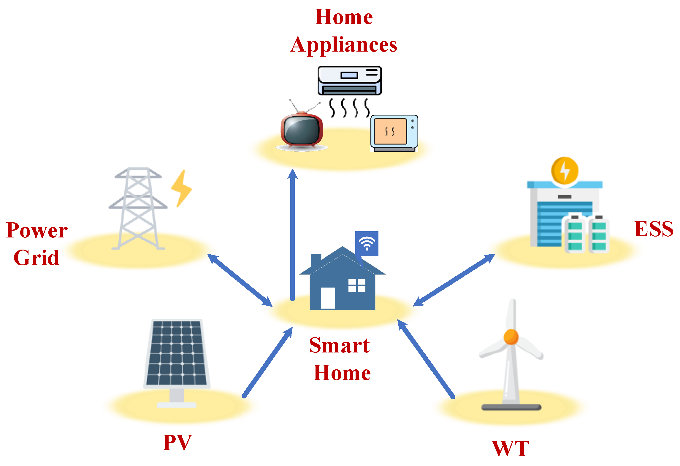
• The suggested HEMS integrates diverse energy resources, such as PV, WT, ESS, and the upstream grid. In order to reduce economic costs, the capabilities of ESS in charging/discharging can shift the load demand into the low-tariff periods;
• A multi-objective model with three different objective functions is made to optimize electricity cost, PAR, and emissions simultaneously. The proposed model can balance the minimization of the proposed three goals together according to the user’s policies. To achieve this optimal balance, a detailed operation is provided for the appliance scheduling, charging/discharging status of ESS, the use of PV, and WT, and also the buying and selling energy in each interval;
• Different electricity prices for bought energy from PV, WT, and upstream are considered. Also, the bought energy from PV, WT, and upstream are specified separately;
• The impacts of diverse weight factors in the multi-objective problem to control the proposed three objective functions—electricity cost, PAR, and emissions—are considered for economic, technical, and environmental benefits. Multi-objective optimization using the weight method allows the users to set trade-offs among the energy costs, PAR, and emissions based on their policies;
• The Pareto-based multi-objective IGWO is considered to extract the possible solutions for the proposed HEMS.

The remaining sections of this paper are presented as follows. The suggested HEMS and problem formulation are illustrated in Section 2, which considers the three suggested objective functions: electricity cost, PAR, and emission, as well as constraints. The GWO and the suggested modification are presented in Section 3. Details of the system and simulation results are considered in Section 4. Finally, the main conclusion and plans are presented in Section 5.

2. Problem Formulation

Figure 1 shows a schematic representation of a HEMS which combines several components such as home appliances, ESS, PV, and WT to prepare a sustainable and efficient energy supply for households. HEMS collects data on the energy consumption of appliances, the state of charge (SoC) of ESS, the PV and WT generation, and electricity prices of PV, WT, and upstream grid. HEMS is integrated into the suggested scheme to provide optimal operation of ESS via control signals based on the information analyzed. In addition, the suggested HEMS allows users to buy and sell energy in a flexible manner with the upstream grid. The smart meter is used to facilitate the communication between HEMS and the SG which includes PV and WT. The amount of energy demand of smart homes is met by the PV, WT, and the upstream grid, and also the stored energy of the ESS. Another benefit of the DRP scheme is selling surplus energy to the upstream grid and generating revenue in this way.

Figure 1. Suggested smart home scheme.

The suggested HEMS scheme includes 24 time steps in a day (T = 24). The decision variables are shiftable appliance usage times, charging and discharging rate of ESS, bought power form PV, WT, and upstream. Three objective functions are defined to minimize cost, PAR, and emissions. Hence, first, the decision variable and constrains of each component are defined in Section 2.1, Section 2.2, Section 2.3, Section 2.4, Section 2.5, Section 2.6 and Section 2.7, and finally, the objective functions are introduced in Section 2.8.

2.1. Load Classification

Electrical appliances in smart homes are classified into three main classes based on their energy consumption and operation mode: interruptible, uninterruptible, and non-shiftable appliances [37]. Each class is described in the following.

2.1.1. Interruptible Appliances

Interruptible appliances are those whose usage time can be changed and which can also be turned off and on during use in order to change the usage time. The total used power of interruptible appliances is specified as below:

$$P_{IA}\left(t\right)={\sum }_{k\in IA}P{R}_k\ast U_k,$$

(1)

where $IA$ shows a set of interruptible appliances; $P_{IA}\left(t\right)$ indicates the total used power of interruptible appliances at time t; $k$ is the number of interruptible appliances; $P{R}_k$ shows the power rating of each interruptible appliance; and $U_k\left(t\right)$ shows the on/off state of each interruptible appliance within period $T$ as follows:

$$U_k=\left\{\begin{array}{c}0 if appliance is OFF\\ 1 if appliance is ON\end{array}\right.,$$

(2)

2.1.2. Uninterruptible Appliances

The time period for using uninterrupted appliances can be changed to another time period, and their operation is continuous and cannot be disconnected during use. The total used power of uninterruptible appliances can be obtained by Equation (3) as follows:

$$P_{UIA}\left(t\right)={\sum }_{l\in UIA}P{R}_l\left(t\right)\ast U_l,$$

(3)

where UIA shows a set of uninterruptible appliances; $P_{UIA}\left(t\right)$ shows the total used power of uninterruptible appliances at time t; $l$ is the number of uninterruptible appliances; $P{R}_l$ is the power rating of each uninterruptible appliance; and $U_l$ is the on/off state of each uninterruptible appliance within the period $T$, and can be represented as

$$U_l=\left\{\begin{array}{c}0 if appliance is OFF\\ 1 if appliance is ON\end{array}\right.,$$

(4)

2.1.3. Non-Shiftable Appliances

The operating pattern of non-shiftable appliances is fixed and unchangeable. The total used power of non-shiftable appliances can be calculated by Equation (5) as

$$P_{NSA}\left(t\right)={\sum }_{q\in NSA}P{R}_q\left(t\right)\ast U_q,$$

(5)

where NSA is a set of non-shiftable appliances; $P_{NSA}\left(t\right)$ is the entire used power of non-shiftable appliances at time t; $q$ shows the number of non-shiftable appliances; $P{R}_q$ shows the power rating of each non-shiftable appliance; and $U_q$ displays the on/off state of each non-shiftable appliance within the period $T$, which is expressed as below:

$$U_q=\left\{\begin{array}{c}0 if appliance is OFF\\ 1 if appliance is ON\end{array}\right.,$$

(6)

Finally, the required total energy for home appliances is obtained as below:

$$P_{app}\left(t\right)=P_{IA}\left(t\right)+P_{UIA}\left(t\right)+P_{NSA}\left(t\right),$$

(7)

where $P_{app}\left(t\right)$ is the sum of required power for home appliances.

2.2. Grid Modeling

The proposed HEMS is able to buy and sell energy to the upstream grid. Utility companies typically limit the amount of electricity a home can exchange with the upstream grid due to distribution grid limitations or contractual agreements. Hence, the grid model can be formulated as below [38,39]:

$$0\le P_{G2H}\left(t\right)\le mod{e}_{G2H}\left(t\right).P_{G2H}^{max},$$

(8)

$$0\le P_{H2G}\left(t\right)\le mod{e}_{H2G}\left(t\right).P_{H2G}^{max},$$

(9)

where $P_{G2H}\left(t\right)$ and $P_{H2G}\left(t\right)$ show the grid-to-home (G2H) and home-to-grid (H2G) powers at period $t$, respectively; $P_{G2H}^{max}$ and $P_{H2G}^{max}$ show the maximum exchanged power between home and upstream grid; and $mod{e}_{H2G}\left(t\right)$ and $mod{e}_{G2H}\left(t\right)$ indicate the H2G and G2H modes at time step $t$, respectively, which are the binary variables.

In general, energy buying and selling cannot be carried out simultaneously, so these constraints are presented by Equation (10) below [38,39]:

$$0\le mod{e}_{G2H}\left(t\right)+mod{e}_{H2G}\left(t\right)\le 1,$$

(10)

2.3. PV System

The azimuth and slope of PV panels are impacted on their output power, which are used to define the solar radiation profile on them. $I^d\left(t\right)$ can be specified via the PVGIS which includes the database of solar radiation [40]. $P_{PV}^d\left(t\right)$ is the output power of PV of the $d^{th}$ day at time-step $t$, which can be calculated by Equation (11) as follows:

$$P_{PV}^d\left(t\right)=P_{PV}^{nominal}\left({\displaystyle \frac{I^d\left(t\right)}{I^T}}\right),$$

(11)

where $P_{PV}^{nominal}$ is the nominal power volume of the PV array; $I^T$ shows the incident radiation at the standard test conditions and its amount is $1 \mathrm{k}\mathrm{W}{\mathrm{m}}^{-2}$.

2.4. WT Model

The output power of WT is modeled according to the various velocities of wind, which is presented as follows [41]:

$$P_{WT}\left(v\right)=\left\{\begin{array}{c}{P}_r v_r<v\le v_0\\ P_r\ast g\left(v\right) v_i<v\le v_r\\ 0 v\le v_i or v>v_0\end{array}\right.,$$

(12)

where $P\left(v\right)$ shows the power curve of WT, which fluctuates based on wind velocity; $P_r$ is the rated power; $v_o, v_r$, and $v_i$ are the cut-off speed, rated speed, and cut-in speed, respectively; g(v) represents an increasing coefficient from zero to one over a time interval that depends on the characteristics of the WT. When the wind speed is between the cut-off and rated speed, the WT’s output power reaches its maximum value.

2.5. ESS

To take advantage of the economic and technical advantages of ESSs, they are integrated into SGs and smart homes. Depending on the charging or discharging mode, the status of ESSs changes as an energy consumer or producer; hence, when the ESS is charged, it is considered as the energy consumer, and on the contrary, when it is in the discharging mode, it is considered as an energy resource. The rated power of the ESS represents the maximum amount of charging and discharging energy in the ESSs, which is shown below:

$$0\le P_{ESS}^{ch}\left(t\right)\le mod{e}_{ESS}^{ch}\left(t\right).P_{ESS}^{ch,max},$$

(13)

$$0\le P_{ESS}^{dis}\left(t\right)\le mod{e}_{ESS}^{dis}\left(t\right).P_{ESS}^{dis,max},$$

(14)

where $P_{ESS}^{ch}\left(t\right)$ and $P_{ESS}^{dis}\left(t\right)$ present the charging and discharging powers of the ESS at time step $t$, respectively; $P_{ESS}^{ch,max}$, and $P_{ESS}^{dis,max}$ show the maximum amount of charging and discharging power of the ESS, respectively; $mod{e}_{ESS}^{ch}\left(t\right)$ and $mod{e}_{ESS}^{dis}\left(t\right)$ represent the charging and discharging conditions of the ESS at time step $t$, respectively, which are the binary variables.

Given that the ESS can only be in one of the charging or discharging states, we have

$$0\le mod{e}_{ESS}^{ch}\left(t\right)+mod{e}_{ESS}^{dis}\left(t\right)\le 1,$$

(15)

The stored energy volume in the ESS is modeled by Equation (16) as follows [42,43]:

$${SoC}_{ESS}\left(t\right)={SoC}_{ESS}\left(t-1\right)+{\eta }_{ESS}.P_{ESS}^{ch}\left(t\right)-{\displaystyle \frac{P_{ESS}^{dis}\left(t\right)}{{\eta }_{ESS}}},$$

(16)

where ${SoC}_{ESS}\left(t\right)$ is the state of charge of ESS that is the volume of energy accumulated in the ESS at time step $t$; ${\eta }_{ESS}$ indicates the charging and discharging efficiency of the ESS. The maximum and minimum capacity of ESS is restricted by Equation (17):

$$\left(1-Do{D}_{ESS}\right).So{C}_{Ess}^{max}\le So{C}_{ESS}\le SO{C}_{ESS}^{max},$$

(17)

where $So{C}_{Ess}^{max}$ shows the maximum volume of the ESS; $Do{D}_{ESS}$ represents the ESS’s depth of discharge (DoD). Here, we assume that the SoC of ESS is minimum at the first time slot and also that it should be minimum at the end of the day [44].

2.6. Energy Balance

All the energy required to feed the loads as well as charge the ESS in the smart home must be provided in the suggested HEMS, so in order to have a balance between consumption and provided energy from the resources, we have [45,46]

$$P_{app}\left(t\right)+P_{ESS}^{Ch}=P_{PV}\left(t\right)+P_{WT}\left(t\right)+P_{G2H}\left(t\right)+P_{ESS}^{dis},$$

(18)

2.7. Selling Balance

When the amount of discharge energy of ESS is greater than the amount of energy required by the home appliances, energy is sold from the smart home to the upstream grid, so we have

$$\left\{\begin{array}{c}{P}_{H2G}\left(t\right)=P_{ESS}^{dis}\left(t\right)-P_{app}\left(t\right) if P_{ESS}^{dis}\left(t\right)>P_{app}\left(t\right) \\ P_{H2G}\left(t\right)=0 if P_{ESS}^{dis}\left(t\right)\le P_{app}\left(t\right)\end{array}\right.,$$

(19)

2.8. Objective Functions

In this subsection, the three main objectives such as electricity cost, PAR, and emission are presented, which must be minimized subject to the constraints of Equations (1)–(19).

2.8.1. Objective Function-1: Electricity Cost

To minimize electricity costs, the below objective is presented:

$$O{F}_1=\min cost={\sum }_{t=1}^{24}{P}_{PV}\left(t\right)\ast Pric{e}_{PV}+P_{WT}\left(t\right)\ast Pric{e}_{WT}+P_{G2H}\left(t\right)\ast Pric{e}_{G2H}\left(t\right)-P_{H2G}\left(t\right)\ast Pric{e}_{H2G},$$

(20)

where $Pric{e}_{PV}$, $Pric{e}_{WT}$, and $Pric{e}_{G2H}\left(t\right)$ are the electricity costs of power of PV, WT, and upstream, respectively; $Pric{e}_{H2G}$ shows the electricity cost of selling power from the smart home to SG.

2.8.2. Objective Function-2: PAR

To increase the stability of the grid, it is essential to minimize the PAR as a technical factor. The second objective function can be obtained mathematically by Equation (21):

$$O{F}_2=\min PAR={\displaystyle \frac{{(\max P_{demand}\left(t\right))}^2}{{\left(avg\left(P_{demand}\right(t\left)\right)\right)}^2}},$$

(21)

where $P_{demand}\left(t\right)$ is the required power demand for smart home at each interval $t$ that can be computed as follows:

$$P_{demand}\left(t\right)=P_{PV}\left(t\right)+P_{WT}\left(t\right)+P_{G2H}\left(t\right)+P_{ESS}^{Ch}-P_{ESS}^{dis}-P_{H2G}\left(t\right),$$

(22)

2.8.3. Objective Function-3: Pollution

The third objective function is defined to decrease pollution, hence the most serious pollutants such as $\mathrm{C}{\mathrm{O}}_2$, $\mathrm{S}{\mathrm{O}}_2$, and $\mathrm{N}{\mathrm{O}}_{\mathrm{x}}$ are considered, so we have

$$O{F}_3=\min pollution={\sum }_{t=1}^{24}Emissio{n}_{grid}\left(t\right)+Emissio{n}_{ESS}\left(t\right),$$

(23)

$$Emissio{n}_{grid}\left(t\right)=P_{G2H}\left(t\right)\ast [E_G^{c{o}_2}+E_G^{s{o}_2}+E_G^{N{O}_x}],$$

(24)

$$Emissio{n}_{ESS}\left(t\right)=P_{ESS}^{dis}\left(t\right)\ast [E_{ESS}^{c{o}_2}+E_{ESS}^{s{o}_2}+E_{ESS}^{N{O}_x}],$$

(25)

where $Emissio{n}_{grid}\left(t\right)$ and $Emissio{n}_{ESS}\left(t\right)$ define the pollutants’ emission in kg/MWh from the grid and ESS, respectively. The $\mathrm{C}{\mathrm{O}}_2$ emission from the grid and ESS are represented as $E_G^{c{o}_2}$ and $E_{ESS}^{c{o}_2}$, respectively. The ${\mathrm{S}\mathrm{O}}_2$ emission from the grid and ESS are shown as $E_G^{s{o}_2}$ and $E_{ESS}^{s{o}_2}$ respectively. $E_G^{N{O}_x}$ and $E_{ESS}^{N{O}_x}$ are the $\mathrm{N}{\mathrm{O}}_{\mathrm{x}}$ emission from the grid and ESS, respectively.

2.8.4. Multi-Objective: Weighting Factors

To solve the suggested multi-objective problem, the weighting ratio method is used to optimize the three mentioned objective functions, so we have

$$O{F}_{total}=w_1.O{F}_1+w_2.O{F}_2+w_3.O{F}_3,$$

(26)

where, $O{F}_{total}$ is the total objective function; $w_1$, $w_2$, and $w_3$ are the weighting ratio of $O{F}_1$, $O{F}_2$, and $O{F}_3$, respectively.

3. Grey Wolf Optimizer

One of the popular swarm intelligence optimization algorithms is GWO, which is inspired by the grey wolf pack in hunting [47]. The simulated wolves are used to iteratively amend solutions to a given problem using social hierarchy and mathematical modeling. To solve optimization problems, this method is used to find the best solutions. A GWO simulates how grey wolves hunt by tracking, encircling, and attacking prey when working together. Hence, by cooperating with the various kinds of wolves together, better solutions are found. In order to update and amend the solutions of the current process, the hunting behavior of the wolves is mathematically modeled. In this procedure, the first top best solutions are determined as alpha ($\alpha$), beta ($\beta$), and delta ($\delta$), respectively, and the rest solutions are specified as omega ($\omega$).

3.1. GWO Mathematical Formulation

Firstly, a population set is created in the domain of lower and upper bounds randomly, which are represented by grey wolves. Also, these wolves can be a potential solution for the optimization problem. Each wolf position is related to each candidate’s solutions in the search space. An objective function is utilized for the optimization problem to determine the fitness of each wolf. An assessment of the quality of a solution according to the goals of the problem is made through this function. A wolf with a better fitness score is considered a better solution. Equations (27) and (28) represent the model of encircling the prey:

$$\overrightarrow{D}=\left|C.X_p-\overrightarrow{X}\left(i\right)\right|,$$

(27)

$$\overrightarrow{X}(i+1)=\overrightarrow{X_p}\left(i\right)-A.\overrightarrow{D},$$

(28)

where $i$ shows the current iteration; $A$ and $C$ represent the coefficient vectors; $X_p$ and $\overrightarrow{X}$ show the position vector of the prey and the grey wolf, respectively. Thus, to compute the amounts of $A$ and $C$, Equations (29)–(31) are presented as follows:

$$A=2b{r}_1-b,$$

(29)

$$C=2r_2,$$

(30)

$$b=2(1-{\displaystyle \frac{i}{ite{r}_{max}}}),$$

(31)

where $r_1$ and $r_2$ represent the random numbers in the range of zero to one; $b$ is a coefficient between two and 0zerothat is linearly decreased from two to zero in each iteration; $ite{r}_{max}$ is the maximum iteration. In order to update the population, the first three best solutions are selected as alpha ($\overrightarrow{X_{\alpha }}$), beta ($\overrightarrow{X_{\beta }}$), and delta ($\overrightarrow{X_{\delta }}$) wolves, respectively, so we have

$$\overrightarrow{X_1}=\overrightarrow{X_{\alpha }}-A_1\overrightarrow{D_{\alpha }},$$

(32)

$$\overrightarrow{X_2}=\overrightarrow{X_{\beta }}-A_2\overrightarrow{D_{\beta }},$$

(33)

$$\overrightarrow{X_3}=\overrightarrow{X_{\delta }}-A_3\overrightarrow{D_{\delta }},$$

(34)

where $\overrightarrow{D_{\alpha }}$, $\overrightarrow{D_{\beta }}$, and $\overrightarrow{D_{\beta }}$ are obtained by Equations (35)–(37):

$$\overrightarrow{D_{\alpha }}=|C_1.\overrightarrow{X_{\alpha }}-\overrightarrow{X}|,$$

(35)

$$\overrightarrow{D_{\beta }}=|C_2.\overrightarrow{X_{\beta }}-\overrightarrow{X}|,$$

(36)

$$\overrightarrow{D_{\delta }}=\left|C_3.\overrightarrow{X_{\delta }}-\overrightarrow{X}\right|.$$

(37)

The positions of all populations are updated according to the positions of the first best solution that are selected as alpha, beta, and delta wolves.

This behavior is inspired by the way wolves in a pack follow leaders. The below mathematical equation is used to guide the movements of wolves’ pack and also balance the exploration of GWO:

$$\overrightarrow{X_H}\left(i+1\right)={\displaystyle \frac{\overrightarrow{X_1}+\overrightarrow{X_2}+\overrightarrow{X_3}}{3}}.$$

(38)

3.2. Improvement Procedure

In this section, an improvement step is added to the GWO to increase its efficiency in finding the optimal solution. The improvement is inspired by the competition between grey wolves to preserve their prey and the efforts of other wild animals, including hyenas, to steal all or part of the prey. Assuming that the attacking group consists of three wild animals attempting to steal and separate a portion of the prey, we have

$$\overrightarrow{R_1}=r_3(X_p-\overrightarrow{X_{R_1}}(i\left)\right),$$

(39)

$$\overrightarrow{R_2}=r_4(X_p-\overrightarrow{X_{R_2}}(i\left)\right),$$

(40)

$$\overrightarrow{R_3}=r_5(X_p-\overrightarrow{X_{R_5}}(i\left)\right),$$

(41)

where $r_3$, $r_4$, and $r_5$ represent the random numbers in the range of zero to one; $\overrightarrow{X_{R_1}}\left(i\right)$, $\overrightarrow{X_{R_2}}\left(i\right)$, and $\overrightarrow{X_{R_3}}\left(i\right)$ are three wild robber animals that are selected randomly in the population. So, separating and stealing a piece of prey is modeled as follows:

$$\overrightarrow{X_R}(i+1)=\overrightarrow{X_R}\left(i\right)-b_R.(\overrightarrow{R_1}+\overrightarrow{R_2}+\overrightarrow{R_3}),$$

(42)

$$b_R=1-{\displaystyle \frac{i}{ite{r}_{max}}},$$

(43)

where $b_R$ is a coefficient between one and zero that is linearly decreased from one to zero in each iteration.

So, assuming a 50% chance for grey wolves to keep the prey they have killed and a 50% chance for the robber, we have

$$\overrightarrow{X}{\displaystyle (i+1)}=\left\{\begin{array}{c}\overrightarrow{X_H}(i+1) if chance>0.5\\ \overrightarrow{X_R}(i+1) if chance\le 0.5\end{array}\right.,$$

(44)

where $chance$ is a random number between zero and one.

The pseudocode of the suggested IGWO to solve the proposed optimization problem is described in Table 1.

Table 1. Pseudo code of the suggested IGWO algorithm.

Start IGWO Algorithm
Input initial variables and constraints such as demand of non-shiftable loads, power rating and usage time of shiftable appliances, energy price of PV, WT, selling and upstream, available power of RERs, charging and discharging rate of ESS, SoC of ESS, emission details for each resource, maximum iteration, number of populations, weighting ratios, etc.
Generate the initial population randomly.
Calculate the total objective function based on Equation (26) subject to the constraints of Equations (1)–(19).
	For $iteration=1:ite{r}_{max}$:
		For each population:
			Select the current population as prey $X_p$;
GWO Phase			Select the best three populations as the alpha ${\displaystyle \left(\overrightarrow{X_{\alpha }}\right)}$, beta ${\displaystyle \left(\overrightarrow{X_{\beta }}\right)}$, and delta ${\displaystyle \left(\overrightarrow{X_{\delta }}\right)}$ wolves, respectively;
			Update the GWO parameters (A, C, b) based on Equations (29)–(31);
			Calculate the first new population ($\overrightarrow{X_H}$) by Equations (32)–(38);
Improvement Phase			Select three populations by random as the wild robber animals $(\overrightarrow{X_{R_1}}{\displaystyle (i)}$, $\overrightarrow{X_{R_2}}{\displaystyle (i)}$, and $\overrightarrow{X_{R_3}}{\displaystyle (i)})$;
			Update the improvement parameters $b_R$ (Equation (43)) and $chance$;
			Calculate the second new population ($\overrightarrow{X_R}$) by Equations (39)–(42);
			Update the new population by Equation (44):
			$if Chance\le 0.5$
				$\overrightarrow{X}(i+1)=\overrightarrow{X_R}$,  else
				$\overrightarrow{X}(i+1)=\overrightarrow{X_H}$
			End if
			Calculate the total objective function for new population $\overrightarrow{X}(i+1)$ based on Equation (26) subject to the constraints of Equations (1)–(19);
			If the new total objective function is lower than the total objective function of current population
				Replace the current population by the new population
			End if
	End for
	Chose the best member as the solution
End IGWO Algorithm

4. Simulation Results

In this section, the suggested SHEM and IGWO are analyzed and validated by considering the energy price of PV, WT, and upstream grid, price of sold energy, energy consumption, and ESS for smart homes. The simulations are implemented for one day with a one-hour time step; hence, HEMS and appliance scheduling are considered in 24 intervals. The IGWO is used to solve the HEMS problem. The simulations are carried out on a 64-bit Intel (R) Core (TM) i7-4600 CPU at 2.1 GHz with 12 GB RAM.

4.1. Input Data

As shown in Figure 1, the smart home consists of ESS and different kinds of appliances such as shiftable and non-shiftable loads, which are connected to an SG that includes PV and WT. An IGWO is used to solve the proposed SHEM system and schedule the appliances in the smart home to decrease the electricity cost, PAR, and emissions simultaneously. The availability of PV and WT powers, the prices of power of PV, WT, and upstream grid, and the emissions of resources, and also the preferred time window, power rating, and operation period for each appliance are specified as the inputs of IGWO for optimizing the proposed objective functions.

Depending on how consumers use the appliances, the time window and interval are framed. Smart homes periodically receive tariffs from the SG and schedule appliances accordingly based on maximum power availability.

The operation period, preferred time window, and power rating of different kinds of appliances such as interruptible, uninterruptible, and non-shiftable appliances are given in Table 2. Table 3 shows the details of the hourly electricity tariff of the upstream grid [48]. Table 4 shows the available power of PV and WT for a day. The electricity prices of PV and WT are 5 cents and 4 cents per kWh, respectively, and also the energy sales rate from the smart home to the grid is set at 4.5 cents per kWh [41]. Table 5 illustrates the emission coefficient (kg/kWh) of diverse pollutants for upstream, ESS, PV, and WT [49]. The details of ESS are presented in Table 6.

Table 2. Details of home appliances.

Category of Appliance	No.	Appliances	Starting Time (h)	Ending Time (h)	Duration of Operation (h)	Power Rating (kW)
Non-shiftable	1	Lighting	18	24	7	0.1
	2	Illumination	20	24	5	0.5
	3	Security Camera	1	24	24	0.2
	4	Refrigerator	1	24	24	0.2
Uninterruptible	5	Washing machine	9	12	2	1.8
	6	Rice cooker	11	15	1	2.1
	7	Dishwasher	9	17	1	1.7
	8	Microwave	7	9	1	1.7
	9	Cooker hood	17	19	1	0.2
	10	Oven	15	19	2	2.5
	11	TV	19	24	5	0.3
	12	Blender	9	18	2	0.3
	13	Vacuum cleaner	7	20	2	1
	14	Music player	7	9	1	0.2
	15	Iron	9	20	2	2.7
	16	Other occasional loads	1	24	5	3
Interruptible	17	Air conditioner-1	14	24	7	2.7
	18	Air conditioner-2	1	8	4	1.6
	19	Water Heater	1	24	4	1.7
	20	Water Pump	1	24	8	1
	21	Laptop	9	23	6	0.1

Table 3. Details of hourly electricity tariff of the upstream grid.

Hour	1	2	3	4	5	6	7	8	9	10	11	12
Cost (Cents/kWh)	3.26	3.08	2.9	2.68	2.62	2.61	2.56	2.52	2.3	2.47	2.32	2.3
Hour	13	14	15	16	17	18	19	20	21	22	23	24
Cost (Cents/kWh)	2.05	2.1	2.41	2.51	2.45	2.33	2.48	3.14	3.5	4.6	5.5	5.06

Table 4. Availability power of PV and WT for a day.

Hour	1	2	3	4	5	6	7	8	9	10	11	12
PV (kW)	0	0	0	0	0	0	0	0.85	2.4	3.4	4	3.65
WT (kW)	3.3	3.1	3.6	4	4	3.8	3.6	3.55	3.65	3.85	4.05	4.2
Hour	13	14	15	16	17	18	19	20	21	22	23	24
PV (kW)	3.25	3	3.35	2.5	1.3	0.15	0	0	0	0	0	0
WT (kW)	4.9	5.3	5.25	5.1	4.85	4.7	4.4	4.2	4.05	3.9	3.75	3.6

Table 5. Emission coefficient of diverse resources.

Resource	$\mathbf{C}{\mathbf{O}}_2$ (kg/kWh)	$\mathbf{S}{\mathbf{O}}_2$ (kg/kWh)	$\mathbf{N}{\mathbf{O}}_{\mathbf{x}}$ (kg/kWh)
Grid	0.95	5 × 10−4	0.0021
ESS	0.01	2 × 10−7	1 × 10−6
WT	0	0	0
PV	0	0	0

Table 6. ESS parameters.

Parameters	${\mathit{P}}_{\mathit{E}\mathit{S}\mathit{S}}^{\mathit{C}\mathit{h}}$ (kW)	${\mathit{P}}_{\mathit{E}\mathit{S}\mathit{S}}^{\mathit{d}\mathit{i}\mathit{s}}$ (kW)	$\mathit{S}\mathit{o}{\mathit{C}}_{\mathit{E}\mathit{S}\mathit{S}}^{\mathit{m}\mathit{i}\mathit{n}}$ (kWh)	$\mathit{S}\mathit{o}{\mathit{C}}_{\mathit{E}\mathit{S}\mathit{S}}^{\mathit{m}\mathit{a}\mathit{x}}$ (kWh)	${\mathit{\eta }}_{\mathit{E}\mathit{S}\mathit{S}}$
Value	3	−3	2	8	1

4.2. Case Studies

The energy demand of smart homes is fed by the PV, WT, ESS, and upstream, and the SHEM system is performed and discussed for four different case studies in this subsection. In the first three case studies, the availability of PV, WT, and ESS is investigated, and then in the fourth case that consists of all PV, WT, and ESS simultaneously, the weighting factor of objective functions is considered and analyzed to show the impact of each objective. To solve the proposed optimization problem, GWO, IGWO [50], and the suggested IGWO algorithms are used and compared in order to schedule the appliances. When the ESS is in the discharging mode and the residential consumer is lower than the discharging rate, after the power demand on home appliances is fed by the ESS, the surplus power is sold to the upstream grid.

To show the performance and effectiveness of the suggested layout in optimizing the electricity cost, PAR, and emission, four different cases are considered. In all four cases, the smart home appliances remain the same, but their scheduling varies due to the power availability of RERs and diverse weighting factors in the objective function. The four cases are summarized below:

• Case-1: Appliance scheduling with PV and ESS;
• Case-2: Appliance scheduling with WT and ESS;
• Case-3: Appliance scheduling with PV, WT, and ESS;
• Case-4: Appliance scheduling with PV, WT, and ESS under different weighting factors.

For the first three cases, the weighting factors are $w_1=1$, $w_2=100$, and $w_3=50$. Also, to show the possible solutions, the Pareto front of a multi-objective IGWO is presented. The maximum iteration for the proposed optimization algorithm is 1000, and 20 independent runs are performed for GWO and IGWO to show the performance of each algorithm and compare them together based on four indexes such as best result, worst result, average of results, and standard deviation.

4.2.1. Case 1: Appliance Scheduling with PV and ESS

In this case study, it is assumed that only the PV and ESS are available in the SG, and the proposed HEMS is performed to schedule the appliances. Table 7 shows the performance of GWO, IGWO [50], and suggested IGWO in solving the proposed SHEM system for Case 1. As can be seen, the suggested IGWO has better performance to solve the proposed optimization problem. In order to minimize the total objective function, the best results of the suggested IGWO, IGWO [50], and GWO are 3555.999, 3577.209, and 3562.798, respectively. The suggested IGWO is reduced by 21.21 and 6.799 in comparison to IGWO [50] and GWO, respectively. Also, the average results for suggested IGWO, IGWO [50], and GWO are 3563.778, 3599.282, and 3601.793, respectively, which is 35.504 and 38.015 lower than IGWO [50] and GWO, respectively. Standard deviation of results shows the robustness and proficiency of IGWO in finding the best results, which is 6.117, that is, 4.492 and 37.266 less than the IGWO [50] (10.609) and GWO (43.483), respectively. Finally, the entire electricity cost, PAR, and emission for the best result of the suggested IGWO in Case 1 are 337.535 (cents), 1.359, and 61.651 (kg/kWh), respectively.

Table 7. Suggested SHEM system over 20 independent simulation runs: Case 1.

Results	Total Objective Function			Electricity Cost (Cents)			PAR			Emission (kg/kWh)
	IGWO	GWO	IGWO [50]	IGWO	GWO	IGWO [50]	IGWO	GWO	IGWO [50]	IGWO	GWO	IGWO [50]
Best result	3555.999	3562.798	3577.209	337.535	326.908	333.920	1.359	1.470	1.609	61.651	61.778	61.648
Worst result	3580.379	3716.024	3610.669	227.897	327.833	322.855	1.514	1.378	1.790	61.821	65.007	62.175
Average of results	3563.778	3601.793	3599.282	337.353	335.565	338.163	1.403	1.499	1.729	61.722	62.327	61.764
Standard deviation of results	6.117	43.483	10.609	4.216	6.177	8.901	0.050	0.093	0.060	0.063	0.960	0.161

Figure 2a shows the convergence curves of GWO, IGWO [50], and the suggested IGWO for the best result that is presented in Table 7. The convergence curve of IGWO shows the performance of the suggested modification in improving the results in each iteration. Finally, a better result is found in comparison to GWO and IGWO [50].

Figure 2. Case 1: (a) Convergence curve [50]; (b) Appliance scheduling; (c) Power supplied by the grid, PV, WT, entire bought power, and total loads; (d) SoC of ESS with charging/discharging status; (e) Pareto front of multi-objective IGWO.

The power demand of scheduled appliances with the proposed HEMS is shown in Figure 2b. Figure 2c shows the bought power from PV, upstream, and power demand for total loads. As can be seen, despite the cost of PV being more than upstream, when the PV is available (8 to 18 h), its power is bought to reduce emissions. When the total bought power is greater than the total loads, the ESS is charged (for example, 1 to 4 h), and on the contrary, when the total bought power is lesser than the total loads, the ESS is discharged to feed the loads (for example, 5 and 7 h). The SoC of ESS and the charging/discharging rate are shown in Figure 2d. The possible solution set is extracted by the Pareto front of the multi-objective IGWO and shown in Figure 2e.

4.2.2. Case 2: Appliance Scheduling with WT and ESS

In this case study, it is assumed that only the WT and ESS are available in the SG, and the suggested HEMS is performed to schedule the appliances. Table 8 shows the performance of GWO, IGWO [50], and the suggested IGWO in solving the proposed SHEM system for Case 2. As shown in Table 8, the proposed IGWO has better performance to solve the proposed optimization problem. In order to minimize the total objective function, the best results of the suggested IGWO, IGWO [50], and GWO are 852.1946, 1416.018, and 1240.372, respectively. The suggested IGWO is reduced by 563.823 and 388.1774 in comparison to IGWO [50] and GWO, respectively. Also, the average of results for the suggested IGWO, IGWO [50], and GWO are 1057.414, 1535.612, and 1577.466, respectively, which is 478.198 and 520.052 lower than IGWO [50] and GWO, respectively; hence, the proposed improvement reduces the total objective function by about 31.14% and 32.97% in comparison to IGWO [50] and GWO, respectively. Standard deviation of results shows the robustness and proficiency of IGWO in finding the best results, which it is 93.198 and about 47.02% less than the GWO (175.903), but it is about 33.87% more than the IGWO [50] (61.634). Finally, the entire electricity cost, PAR, and emission for the best result of the suggested IGWO in Case 2 are 364.556 (Cents), 1.341, and 7.070 (kg/kWh), respectively. Availability of WT instead of PV is considered in Case 2; electricity cost and PAR are increased by 11.5% and 1.32%, respectively, and emission is reduced by 88.5%.

Table 8. Suggested SHEM system over 20 independent simulation runs: Case 2.

Results	Total Objective Function			Electricity Cost (Cents)			PAR			Emission (kg/kWh)
	IGWO	GWO	IGWO [50]	IGWO	GWO	IGWO [50]	IGWO	GWO	IGWO [50]	IGWO	GWO	IGWO [50]
Best result	852.1946	1240.372	1416.018	364.556	351.484	347.850	1.341	1.661	1.764	7.070	14.457	17.835
Worst result	1223.883	1888.883	1651.453	360.388	350.360	344.290	1.543	1.599	2.056	14.182	27.572	22.032
Average of results	1057.414	1577.466	1535.612	359.796	346.232	347.009	0.089	1.616	1.839	11.081	21.392	20.092
Standard deviation of results	93.198	175.903	61.634	2.532	4.397	3.494	0.089	0.103	0.164	1.805	3.578	1.113

Figure 3a shows the convergence curves of GWO, IGWO [50], and the suggested IGWO for the best result which is presented in Table 8. The convergence curve of IGWO shows the performance of the suggested modification in improving the results in each iteration. Finally, a better result is found in comparison to GWO.

Figure 3. Case 2: (a) Convergence curve [50]; (b) Appliance scheduling; (c) Power supplied by the grid; PV, WT, entire bought power and total loads; (d) SoC of ESS with charging/discharging status; (e) Sold energy to upstream; (f) Pareto front of multi-objective IGWO.

The power demand of scheduled appliances with the proposed HEMS is shown in Figure 3b. Figure 3c shows the bought power from WT, upstream, and the power demand of total loads. As can be seen, despite the cost of WT being greater than upstream in most hours, the power is bought from WT to reduce emissions. When the total bought power is greater than the total loads, the ESS is charged, and on the contrary, when the total bought power is lesser than the total loads, the ESS is discharged to feed the loads. The SoC of ESS and charging/discharging rate are shown in Figure 3d. As can be seen, it is charged in low price time and discharged in high price time (for example, 23 and 24 h when the upstream price is more than 5 cents). Figure 3e shows the sold power to the SG in the 14th time slots. When the ESS is in the discharge mode, and the total load is lesser than the discharging rate, the surplus power is sold to the SG. The possible solution set is extracted by the Pareto front of the multi-objective IGWO and shown in Figure 3f.

4.2.3. Case 3: Appliance Scheduling with PV, WT, and ESS

In this case study, the RERs such as PV, WT, and also ESS are available in the SG, and the suggested HEMS is performed to schedule the appliances. Table 9 shows the performance of GWO, IGWO [50], and the suggested IGWO in solving the proposed SHEM system for Case 3. As shown in Table 9, the suggested IGWO has better performance to find the best solution. To minimize the total objective function, the best results of the suggested IGWO, GWO, and IGWO [50] are 819.833, 1158.683, and 1033.290, respectively. The suggested IGWO is reduced by 338.85 (about 29.24%) and 213.457 (about 20.66%) in comparison to GWO and IGWO [50], respectively.

Table 9. Suggested SHEM system over 20 independent simulation runs: Case 3.

Results	Total Objective Function			Electricity Cost (Cents)			PAR			Emission (kg/kWh)
	IGWO	GWO	IGWO [50]	IGWO	GWO	IGWO [50]	IGWO	GWO	IGWO [50]	IGWO	GWO	IGWO [50]
Best result	819.833	1158.683	1033.290	375.865	368.226	376.505	1.731	1.648	1.857	5.417	12.512	9.423
Worst result	1076.138	1829.079	1276.016	370.592	353.669	374.393	1.670	1.785	2.296	10.771	25.938	13.440
Average of results	933.996	1320.535	1196.382	379.872	365.570	376.201	1.708	1.737	1.992	7.666	15.625	12.419
Standard deviation of results	70.417	195.049	63.329	5.181	5.973	3.656	0.146	0.113	0.155	1.546	3.889	1.185

Also, the average of results for the suggested IGWO, GWO, and IGWO [50] are 933.996, 1320.535, and 1196.382, respectively, which is 386.539 and 262.386 lower than GWO and IGWO [50], respectively, which means the proposed improvement reduces the total objective function by about 29.27% and 21.93%% in comparison to GWO and IGWO [50], respectively. Standard deviation of results shows the robustness and proficiency of IGWO in finding the best results, which is 70.417 and about 63.89% lesser than the GWO, but it is about 11.19% greater than the IGWO [50]. Finally, the entire electricity cost, PAR, and emission for the best result of the suggested IGWO in Case 3 are 375.865 (cents), 1.731, and 5.417 (kg/kWh), respectively.

Figure 4a depicts the convergence curves of GWO and IGWO for the best result that is presented in Table 9. The convergence curve of IGWO shows the performance of the suggested modification in improving the results in each iteration. Finally, a better result is found in comparison to GWO. The power demand of scheduled appliances with the proposed HEMS is shown in Figure 4b. Figure 4c shows the bought power from WT, upstream, and the power demand of total loads. As can be seen in Figure 4c, most of the bought power is when both PV and WT are available. When the total bought power is greater than the total loads, the ESS is charged (for example, in 1 to 3 h), and on the contrary, when the total bought power is lesser than the total loads (for example, in 22 to 24 h), the ESS is discharged to feed the loads. The SoC of ESS and charging/discharging rate are shown in Figure 4d. The possible solution set is extracted by the Pareto front of the multi-objective IGWO and shown in Figure 4e.

Figure 4. Case 3: (a) Convergence curve [50]; (b) Appliance scheduling; (c) Power supplied by the grid, PV, WT, entire bought power and total loads; (d) SoC of ESS with charging/discharging status; (e) Pareto front of multi-objective IGWO.

By comparing the solution set that is shown in Figure 2e, Figure 3f and Figure 4e and the results presented in Table 7, Table 8 and Table 9 which are obtained by weighting factors, it is obvious that by adjusting the weighting factors for reaching specific goals, the algorithm can obtain the results which are not extracted by the Pareto front method.

4.2.4. Case 4: Appliance Scheduling with PV, WT, and ESS Under Different Weighting Factors

In this case study, the suggested HEMS is performed to schedule the appliances under different weighting factors to show the impacts of each objective function, while PV, WT, and ESS are investigated in the SG simultaneously. Table 10 shows the performance of GWO and IGWO to solve the proposed SHEM system for Case 4 under different weighting factors. As shown in Table 10, the proposed IGWO has better performance to find the best solution, has better result in worst results, and also the average of results is lower than that of GWO under different weighting factors. Furthermore, the standard deviation of IGWO is lower than that of GWO, which shows the robustness and proficiency of IGWO in finding the results. Table 11 shows the exchanged power between smart home and SG-based best results which is shown in Table 10.

Table 10. Suggested SHEM system over 20 independent simulation runs: Case 4.

${\mathit{w}}_1$	${\mathit{w}}_2$	${\mathit{w}}_3$	Index	Algorithm	Objective Functions
					Total Objective Function	Cost (Cents)	PAR	Emission (kg/kWh)
1	0	0	Best Result	IGWO	198.972	198.972	3.169	99.955
				GWO	210.937	210.938	4.004	92.118
			Worst Result	IGWO	217.522	217.522	3.315	93.238
				GWO	221.4659	221.465	3.529	89.574
			Average	IGWO	205.236	205.236	3.469	98.269
				GWO	215.114	214.114	3.450	91.792
			Standard deviation	IGWO	3.897	3.897	0.366	1.517
				GWO	2.974	2.974	0.271	1.446
1	50	0	Best Result	IGWO	302.997	237.622	1.307	90.732
				GWO	302.629	229.486	1.463	90.318
			Worst Result	IGWO	319.436	245.105	1.487	84.549
				GWO	319.731	255.238	1.290	83.146
			Average	IGWO	311.287	244.722	1.331	86.203
				GWO	310.884	242.990	1.358	87.154
			Standard deviation	IGWO	4.006	3.857	0.055	3.042
				GWO	4.411	6.401	0.073	2.185
1	100	0	Best Result	IGWO	375.365	255.011	1.204	78.648
				GWO	376.306	245.579	1.307	84.224
			Worst Result	IGWO	389.823	258.283	1.315	79.557
				GWO	396.711	260.101	1.366	82.585
			Average	IGWO	380.540	252.817	1.277	82.417
				GWO	382.306	254.003	1.283	84.394
			Standard deviation	IGWO	3.640	2.736	0.029	2.409
				GWO	5.414	4.957	0.028	2.057
1	50	50	Best Result	IGWO	721.616	373.921	1.897	5.057
				GWO	1069.730	365.749	1.762	12.317
			Worst Result	IGWO	964.632	373.618	1.509	10.311
				GWO	1667.915	360.775	1.995	24.148
			Average	IGWO	837.454	377.825	1.723	7.469
				GWO	1303.952	364.788	1.868	16.915
			Standard deviation	IGWO	79.048	4.359	0.205	1.710
				GWO	193.985	8.616	0.151	3.971
1	50	100	Best Result	IGWO	985.592	388.967	1.689	5.121
				GWO	1695.385	369.159	2.050	12.238
			Worst Result	IGWO	1313.239	376.227	1.756	8.492
				GWO	2694.618	357.418	1.593	22.575
			Average	IGWO	1157.094	381.367	1.846	6.834
				GWO	2070.552	364.776	1.971	16.072
			Standard deviation	IGWO	114.022	3.467	0.139	1.149
				GWO	269.422	4.299	0.207	2.743
1	10	2	Best Result	IGWO	392.442	308.739	1.532	34.189
				GWO	398.335	304.544	1.326	40.268
			Worst Result	IGWO	405.717	300.565	1.702	44.066
				GWO	412.698	291.871	1.791	51.459
			Average	IGWO	396.916	312.090	1.558	34.621
				GWO	403.633	287.937	1.701	49.345
			Standard deviation	IGWO	3.293	8.144	0.104	5.066
				GWO	2.880	8.479	0.133	4.526

Table 11. Exchanged power between smart home and SG based on best results which is mentioned in Table 10.

${\mathit{w}}_1$	${\mathit{w}}_2$	${\mathit{w}}_3$	Method	Bought Power (kW)				Sold Power (kW)
				WT	PV	Upstream	Total
1	0	0	IGWO	1.2481	0.0525	104.739	106.0395	13.5395
			GWO	2.3198	0.4883	96.5865	99.3945	6.8945
1	50	0	IGWO	1.4854	0.0518	95.1434	96.6805	4.1805
			GWO	3.6041	0.6748	94.6819	98.9608	6.4608
1	100	0	IGWO	9.5097	0.5013	82.4890	92.5000	0
			GWO	5.8236	0.5491	88.3323	94.7050	2.2050
1	50	50	IGWO	78.2795	8.9984	5.2222	92.5000	0
			GWO	76.1656	3.5132	12.8212	92.5000	0
1	50	100	IGWO	65.9061	21.2942	5.2997	92.5000	0
			GWO	68.8895	10.8388	12.7717	92.5000	0
1	10	2	IGWO	59.6819	0.1303	35.7459	95.5582	3.0582
			GWO	49.0290	1.2671	42.2038	92.5000	0

When the weighting factors of PAR and emission are zero ($w_2=0$, and $w_3=0$), it means that the SHEM system is solved in a single objective mode, and the goal is the reduction in electricity cost; hence, without considering the PAR and emissions, the electricity cost is reduced to 198.972 cents, but the PAR and emissions are increased to 3.169 and 99.955 (kg/kWh) for the best solution of IGWO, respectively, due to the electricity price of upstream being lower than the electricity price of PV and WT. Hence, as can be seen in Table 11, the bought power from WT, PV, and upstream is 1.2481 kW, 0.0525 kW, and 104.739 kW, respectively, and also the smart home sells 13.5395 kW to the upstream, which means power is bought at a low price time and sold to the upstream at a high price time to diminish the electricity cost for the smart home.

When the weighting factors of emission is zero ($w_3=0$), it means that the SHEM system is solved in a multi-objective mode with two objectives, and the goals are minimizing the electricity cost and PAR. Hence, without considering the emissions, the electricity cost and PAR are optimized to 237.622 cents and 1.307, respectively, for weighting factors $w_1=1$ and $w_2=50$, but the emissions are as high as 90.732 (kg/kWh) for the best solution of IGWO due to the electricity price of upstream being lower than the electricity price of PV and WT. By increasing the weighting factor of the second objective function PAR from 50 to 100, the PAR is reduced from 1.307 to 1.204 (7.88% reduction), but the electricity cost is increased from 237.622 cents to 255.011 (7.32% increase).

By considering all three objective functions, the emissions are reduced, too, and as can be seen in Table 11, most of the bought power is prepared by PV and WT; for example, for $w_1=1$, $w_2=50$, and $w_3=50$, the bought power from WT, PV, and upstream is 78.2795 kW, 8.9984 kW, and 5.2222 kW, respectively, and also the electricity cost, PAR, and emission are 373.921 cents, 1.897, and 5.057 (kg/kWh) for the best results, respectively. Also, by reducing the weighting factor to $w_1=1$, $w_2=10$, and $w_3=2$, the bought power from WT, PV, and upstream is 59.6819 kW, 0.1303 kW, and 35.7459 kW, respectively, and the smart home sells 3.0582 kW to the SG. Furthermore, the electricity cost, PAR, and emission are 308.739 cents, 1.532, and 34.189 (kg/kWh) for the best results, respectively. It can be concluded that the objectives can be adjusted by tuning the weighting factor based on the policies of smart homes.

5. Conclusions

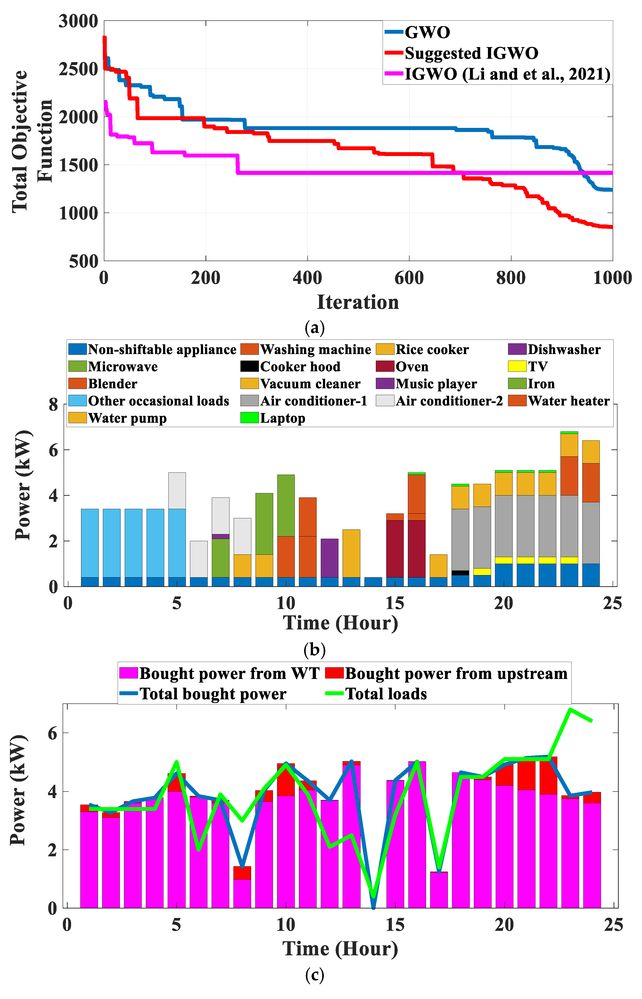
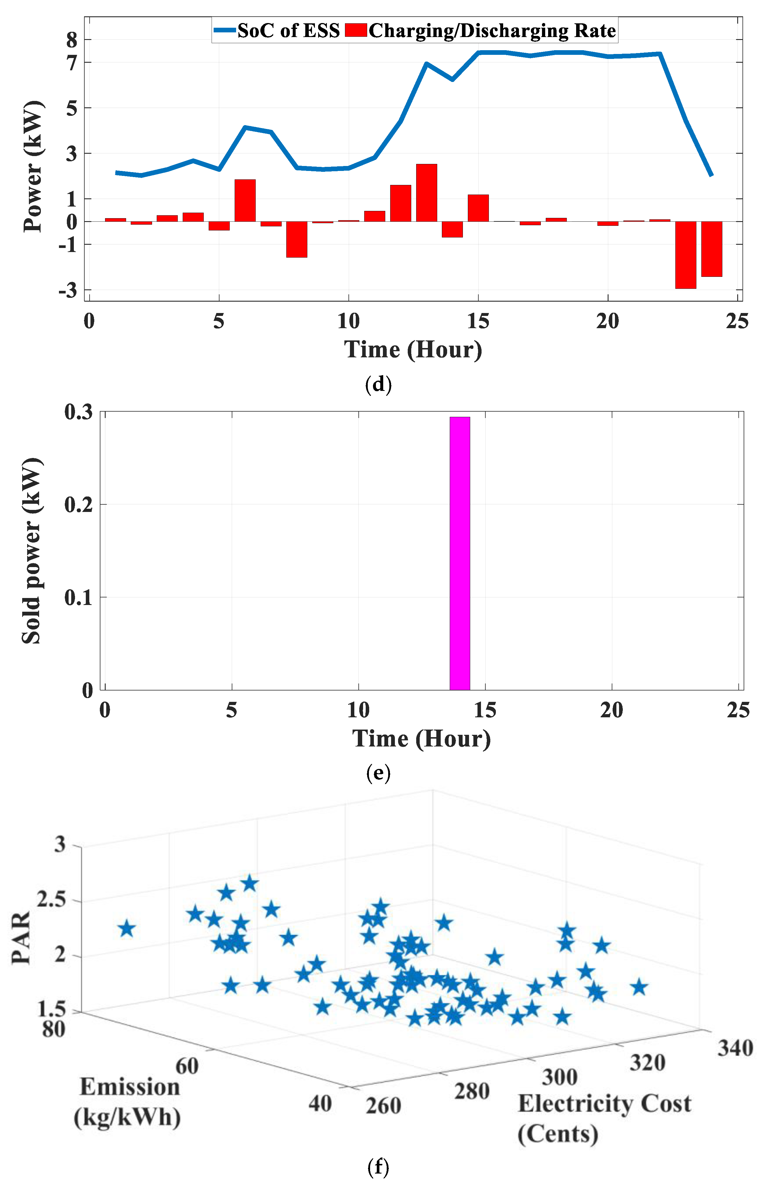
In this study, a novel modification GWO is suggested to solve the SHEM system, which uses the appliance scheduling scheme in smart homes to raise energy efficiency and decrease energy costs, PAR, and emissions in SGs. The developed HEMS model is played as an active prosumer in the energy market and is considered in an SG consisting of PV, WT, and ESS, which is connected to the upstream. Also, the electricity cost of PV, WT, and ToU tariffs for the upstream are considered in the proposed HEMS model. Furthermore, the selling energy from the smart home to SG is considered in the HEMS model: the surplus energy of the ESS is sold to the SG when the home loads are lower than the discharging rate of the ESS. The proposed SHEM system is performed in three cases with the availability of WT and PV in the SG and in one case with different weighting factors to show the impacts of each objective function of the SHEM system. An improved GWO is used to solve the proposed optimization problem. The suggested improvement is inspired by the competition between grey wolves to preserve their prey and the efforts of other wild animals, including hyenas, to steal all or part of the prey. The results in all cases show that the proposed IGWO improves the performance of GWO in finding the best solutions, and also it is more robust and effective with lower standard deviation and average of best results in comparison to GWO. For example, in Case 3, the proposed improvement reduces the total objective function by about 29.27%, and also the standard deviation of results is reduced by 63.89% in comparison to the GWO. For the first three cases, it is shown that by penetrating the PV and WT in SG, emissions are reduced significantly. Also, the goals can be adjusted by weighting factors that can be selected according to the policies of smart homes. By considering only electricity cost as the objective function, the cost is reduced to 198.972 cents, and most of the energy is prepared via the upstream due to the cost of PV and WT being higher than the upstream electricity tariffs in most hours. In addition, by adjusting the weighting factor based on the goals of smart homes, the prepared energy is divided between the resources. Furthermore, the proposed optimization problem is solved by the Pareto front-based multi-objective IGWO to show the possible solution set.

To extend this work, we plan to consider thermal loads, inverter-based air conditioners, and rooftop PV systems for smart homes, and then extend the system to an SG which includes combined-heat power systems, micro-turbines, electric vehicles, parking slots, and heat pumps. Furthermore, the water–energy nexus structure will be considered in the smart energy management system. The uncertainty of generation units, electric vehicles, etc., could be modeled in the optimization problem. Also, to reduce the computation burden and number of variables in the optimization problem, a cloud-fog architecture will be considered.

References

- El-Afifi, M.I.; Sedhom, B.E.; Eladl, A.A.; Elgamal, M.; Siano, P. Demand side management strategy for smart building using multi-objective hybrid optimization technique. Results Eng. 2024, 22, 102265. [Google Scholar] [CrossRef]
- El-Afifi, M.I.; Sedhom, B.E.; Padmanaban, S.; Eladl, A.A. A review of IoT-enabled smart energy hub systems: Rising, applications, challenges, and future prospects. Renew. Energy Focus 2024, 51, 100634. [Google Scholar] [CrossRef]
- Kober, T.; Schiffer, H.W.; Densing, M.; Panos, E. Global energy perspectives to 2060–WEC’s World Energy Scenarios 2019. Energy Strategy Rev. 2020, 31, 100523. [Google Scholar] [CrossRef]
- Amer, A.; Shaban, K.; Gaouda, A.; Massoud, A. Home energy management system embedded with a multi-objective demand response optimization model to benefit customers and operators. Energies 2021, 14, 257. [Google Scholar] [CrossRef]
- Raza, A.; Li, J.; Adnan, M.; Ahmad, I. Optimal load forecasting and scheduling strategies for smart homes peer-to-peer energy networks: A comprehensive survey with critical simulation analysis. Results Eng. 2024, 22, 102188. [Google Scholar] [CrossRef]
- Panah, P.G.; Bornapour, S.M.; Nosratabadi, S.M.; Guerrero, J.M. Hesitant fuzzy for conflicting criteria in multi-objective deployment of electric vehicle charging stations. Sustain. Cities Soc. 2022, 85, 104054. [Google Scholar] [CrossRef]
- Korab, R.; Połomski, M.; Naczyński, T. Optimal Scheduling of Energy Storage and Shiftable Loads in Grid-Connected Residential Buildings with Photovoltaic Micro-Installations. Energies 2024, 17, 5264. [Google Scholar] [CrossRef]
- Iqbal, S.; Sarfraz, M.; Ayyub, M.; Tariq, M.; Chakrabortty, R.K.; Ryan, M.J.; Alamri, B. A comprehensive review on residential demand side management strategies in smart grid environment. Sustainability 2021, 13, 7170. [Google Scholar] [CrossRef]
- Ali, S.; Khan, I.; Jan, S.; Hafeez, G. An optimization based power usage scheduling strategy using photovoltaic-battery system for demand-side management in smart grid. Energies 2021, 14, 2201. [Google Scholar] [CrossRef]
- Zhang, N.; Ochoa, L.F.; Kirschen, D.S. Investigating the impact of demand side management on residential customers. In Proceedings of the 2011 2nd IEEE PES International Conference and Exhibition on Innovative Smart Grid Technologies, Manchester, UK, 5–7 December 2011; IEEE: New York, NY, USA; pp. 1–6. [Google Scholar]
- Tsagarakis, G.; Thomson, R.C.; Collin, A.J.; Harrison, G.P.; Kiprakis, A.E.; McLaughlin, S. Assessment of the cost and environmental impact of residential demand-side management. IEEE Trans. Ind. Appl. 2016, 52, 2486–2495. [Google Scholar] [CrossRef]
- Moradzadeh, B.; Tomsovic, K. Two-stage residential energy management considering network operational constraints. IEEE Trans. Smart Grid 2013, 4, 2339–2346. [Google Scholar] [CrossRef]
- Kinhekar, N.; Padhy, N.P.; Gupta, H.O. Demand side management for residential consumers. In Proceedings of the 2013 IEEE Power & Energy Society General Meeting, Vancouver, BC, Canada, 21–25 July 2013; IEEE: New York, NY, USA; pp. 1–5. [Google Scholar]
- Rastegar, M.; Fotuhi-Firuzabad, M.; Zareipour, H. Home energy management incorporating operational priority of appliances. Int. J. Electr. Power Energy Syst. 2016, 74, 286–292. [Google Scholar] [CrossRef]
- Lokeshgupta, B.; Sivasubramani, S. Multi-objective home energy management with battery energy storage systems. Sustain. Cities Soc. 2019, 47, 101458. [Google Scholar] [CrossRef]
- Javadi, M.S.; Nezhad, A.E.; Nardelli, P.H.; Gough, M.; Lotfi, M.; Santos, S.; Catalão, J.P. Self-scheduling model for home energy management systems considering the end-users discomfort index within price-based demand response programs. Sustain. Cities Soc. 2021, 68, 102792. [Google Scholar] [CrossRef]
- Arun, S.L.; Selvan, M.P. Intelligent residential energy management system for dynamic demand response in smart buildings. IEEE Syst. J. 2017, 12, 1329–1340. [Google Scholar] [CrossRef]
- Carli, R.; Dotoli, M. Decentralized control for residential energy management of a smart users’ microgrid with renewable energy exchange. IEEE/CAA J. Autom. Sin. 2019, 6, 641–656. [Google Scholar] [CrossRef]
- Dinh, H.T.; Yun, J.; Kim, D.M.; Lee, K.H.; Kim, D. A home energy management system with renewable energy and energy storage utilizing main grid and electricity selling. IEEE Access 2020, 8, 49436–49450. [Google Scholar] [CrossRef]
- Rahim, S.; Javaid, N.; Ahmad, A.; Khan, S.A.; Khan, Z.A.; Alrajeh, N.; Qasim, U. Exploiting heuristic algorithms to efficiently utilize energy management controllers with renewable energy sources. Energy Build. 2016, 129, 452–470. [Google Scholar] [CrossRef]
- Shewale, A.; Mokhade, A.; Funde, N.; Bokde, N.D. An overview of demand response in smart grid and optimization techniques for efficient residential appliance scheduling problem. Energies 2020, 13, 4266. [Google Scholar] [CrossRef]
- Javaid, N.; Hussain, S.M.; Ullah, I.; Noor, M.A.; Abdul, W.; Almogren, A.; Alamri, A. Demand side management in nearly zero energy buildings using heuristic optimizations. Energies 2017, 10, 1131. [Google Scholar] [CrossRef]
- Omrany, H.; Chang, R.; Soebarto, V.; Zhang, Y.; Ghaffarianhoseini, A.; Zuo, J. A bibliometric review of net zero energy building research 1995–2022. Energy Build. 2022, 262, 111996. [Google Scholar] [CrossRef]
- Marzband, M.; Alavi, H.; Ghazimirsaeid, S.S.; Uppal, H.; Fernando, T. Optimal energy management system based on stochastic approach for a home Microgrid with integrated responsive load demand and energy storage. Sustain. Cities Soc. 2017, 28, 256–264. [Google Scholar] [CrossRef]
- Molla, T.; Khan, B.; Moges, B.; Alhelou, H.H.; Zamani, R.; Siano, P. Integrated optimization of smart home appliances with cost-effective energy management system. CSEE J. Power Energy Syst. 2019, 5, 249–258. [Google Scholar] [CrossRef]
- Imran, A.; Hafeez, G.; Khan, I.; Usman, M.; Shafiq, Z.; Qazi, A.B.; Khalid, A.; Thoben, K.D. Heuristic-based programable controller for efficient energy management under renewable energy sources and energy storage system in smart grid. IEEE Access 2020, 8, 139587–139608. [Google Scholar] [CrossRef]
- Rocha, H.R.; Honorato, I.H.; Fiorotti, R.; Celeste, W.C.; Silvestre, L.J.; Silva, J.A. An Artificial Intelligence based scheduling algorithm for demand-side energy management in Smart Homes. Appl. Energy 2021, 282, 116145. [Google Scholar] [CrossRef]
- Georgiou, G.S.; Christodoulides, P.; Kalogirou, S.A. Optimizing the energy storage schedule of a battery in a PV grid-connected nZEB using linear programming. Energy 2020, 208, 118177. [Google Scholar] [CrossRef]
- Mouassa, S.; Bouktir, T.; Jurado, F. Scheduling of smart home appliances for optimal energy management in smart grid using Harris-hawks optimization algorithm. Optim. Eng. 2021, 22, 1625–1652. [Google Scholar] [CrossRef]
- Zadehbagheri, M.; Abbasi, A.R. Energy cost optimization in distribution network considering hybrid electric vehicle and photovoltaic using modified whale optimization algorithm. J. Supercomput. 2023, 79, 14427–14456. [Google Scholar] [CrossRef]
- Guo, D.; Li, J.; Zhang, S.; Liu, R.; Sun, F.; Zhang, H.; Ma, P.; Li, J. Cooperative operation strategy of electric vehicle and photovoltaic power station considering carbon reduction benefit under dynamic electricity price. Environ. Sci. Pollut. Res. 2023, 30, 92922–92936. [Google Scholar] [CrossRef] [PubMed]
- Dehghani, M.; Bornapour, S.M. Smart Homes Energy Management: Optimal Multi-Objective Appliance Scheduling Model Considering Electrical Energy Storage and Renewable Energy Resources. Heliyon 2025, 11, e42417. [Google Scholar] [CrossRef]
- Rajagopalan, A.; Nagarajan, K.; Montoya, O.D.; Dhanasekaran, S.; Kareem, I.A.; Perumal, A.S.; Lakshmaiya, N.; Paramasivam, P. Multi-objective optimal scheduling of a microgrid using oppositional gradient-based grey wolf optimizer. Energies 2022, 15, 9024. [Google Scholar] [CrossRef]
- Chen, H.; Gao, L.; Zhang, Z. Multi-objective optimal scheduling of a microgrid with uncertainties of renewable power generation considering user satisfaction. Int. J. Electr. Power Energy Syst. 2021, 131, 107142. [Google Scholar] [CrossRef]
- Nammouchi, A.; Aupke, P.; D’andreagiovanni, F.; Ghazzai, H.; Theocharis, A.; Kassler, A. Robust opportunistic optimal energy management of a mixed microgrid under asymmetrical uncertainties. Sustain. Energy Grids Netw. 2023, 36, 101184. [Google Scholar] [CrossRef]
- Vidan, M.; D’Andreagiovanni, F.; Pandžić, H. Individual thermal generator and battery storage bidding strategies based on robust optimization. IEEE Access 2021, 9, 66829–66838. [Google Scholar] [CrossRef]
- Mahmood, Z.; Cheng, B.; Butt, N.A.; Rehman, G.U.; Zubair, M.; Badshah, A.; Aslam, M. Efficient scheduling of home energy management controller (hemc) using heuristic optimization techniques. Sustainability 2023, 15, 1378. [Google Scholar] [CrossRef]
- Shewale, A.; Mokhade, A.; Funde, N.; Bokde, N.D. A survey of efficient demand-side management techniques for the residential appliance scheduling problem in smart homes. Energies 2022, 15, 2863. [Google Scholar] [CrossRef]
- Panah, P.G.; Hooshmand, R.A.; Gholipour, M.; Bornapour, M. Urban microgrid ancillary service provision using plugin electric vehicle and waste-to-energy CHP. J. Energy Storage 2020, 29, 101413. [Google Scholar] [CrossRef]
- Dinh, H.T.; Kim, D. An optimal energy-saving home energy management supporting user comfort and electricity selling with different prices. IEEE Access 2021, 9, 9235–9249. [Google Scholar] [CrossRef]
- Chakraborty, A.; Ray, S. Multi-objective energy management using a smart charging technique of a microgrid with the charging impact of plug-in hybrid electric vehicles. Sustain. Cities Soc. 2024, 117, 105923. [Google Scholar] [CrossRef]
- Shokri, M.; Niknam, T.; Sarvarizade-Kouhpaye, M.; Pourbehzadi, M.; Javidi, G.; Sheybani, E.; Dehghani, M. A Novel Optimal Planning and Operation of Smart Cities by Simultaneously Considering Electric Vehicles, Photovoltaics, Heat Pumps, and Batteries. Processes 2024, 12, 1816. [Google Scholar] [CrossRef]
- Al Muala, Z.A.; Bany Issa, M.A.; Bello Bugallo, P.M. Integrating Life Cycle Principles in Home Energy Management Systems: Optimal Load PV–Battery–Electric Vehicle Scheduling. Batteries 2024, 10, 138. [Google Scholar] [CrossRef]
- Tostado-Véliz, M.; Gurung, S.; Jurado, F. Efficient solution of many-objective Home Energy Management systems. Int. J. Electr. Power Energy Syst. 2022, 136, 107666. [Google Scholar] [CrossRef]
- Huy, T.H.; Dinh, H.T.; Kim, D. Multi-objective framework for a home energy management system with the integration of solar energy and an electric vehicle using an augmented ε-constraint method and lexicographic optimization. Sustain. Cities Soc. 2023, 88, 104289. [Google Scholar] [CrossRef]
- Akbarizadeh, M.; Niknam, T.; Dehghani, M.; Pourbehzadi, M.; Javidi, G.; Sheybani, E. Multi-Objective Strategic Offering of Networked Energy Hubs in the Day-Ahead Energy Market according to Uncertainty Modelling. Energy 2024, 314, 134288. [Google Scholar] [CrossRef]
- Negi, G.; Kumar, A.; Pant, S.; Ram, M. GWO: A review and applications. Int. J. Syst. Assur. Eng. Manag. 2021, 12, 1–8. [Google Scholar] [CrossRef]
- Kanakadhurga, D.; Prabaharan, N. Smart home energy management using demand response with uncertainty analysis of electric vehicle in the presence of renewable energy sources. Appl. Energy 2024, 364, 123062. [Google Scholar] [CrossRef]
- Sedighizadeh, M.; Fazlhashemi, S.S.; Javadi, H.; Taghvaei, M. Multi-objective day-ahead energy management of a microgrid considering responsive loads and uncertainty of the electric vehicles. J. Clean. Prod. 2020, 267, 121562. [Google Scholar] [CrossRef]
- Li, Y.; Lin, X.; Liu, J. An improved gray wolf optimization algorithm to solve engineering problems. Sustainability 2021, 13, 3208. [Google Scholar] [CrossRef]
Disclaimer/Publisher’s Note: The statements, opinions and data contained in all publications are solely those of the individual author(s) and contributor(s) and not of MDPI and/or the editor(s). MDPI and/or the editor(s) disclaim responsibility for any injury to people or property resulting from any ideas, methods, instructions or products referred to in the content. |
© 2025 by the authors. Licensee MDPI, Basel, Switzerland. This article is an open access article distributed under the terms and conditions of the Creative Commons Attribution (CC BY) license (https://creativecommons.org/licenses/by/4.0/).