Collaborative Forecasting of Multiple Energy Loads in Integrated Energy Systems Based on Feature Extraction and Deep Learning

Abstract

Accurate load forecasting is crucial for the safe, stable, and economical operation of integrated energy systems. However, directly applying single models to predict coupled cooling, heating, and electric loads under complex influencing factors often yields unsatisfactory results. This paper proposes a collaborative load forecasting method based on feature extraction and deep learning. First, the complete ensemble empirical mode decomposition with adaptive noise algorithm decomposes load data, and a dynamic time warping-based k-medoids clustering algorithm reconstructs subsequences aligned with system load components. Second, a correlation analysis identifies the key influencing factors for model input. Then, a multi-task parallel learning framework combining a regression convolutional neural network and long short-term memory networks is developed to predict reconstructed subsequences. Case studies demonstrate that the proposed model achieves mean absolute percentage errors (MAPE) of 2.24%, 2.75%, and 1.69% for electricity, cooling, and heating loads on summer workdays, with mean accuracy (MA) values of 97.76%, 97.25%, and 98.31%, respectively. For winter workdays, the MAPE values are 2.92%, 1.66%, and 2.87%, with MA values of 97.08%, 98.34%, and 97.13%. Compared to traditional single-task models, the weighted mean accuracy (WMA) improves by 2.01% and 2.33% in summer and winter, respectively, validating its superiority. This method provides a high-precision tool for the planning and operation of integrated energy systems.

1. Introduction

Integrated energy systems, which coordinate energy production, transmission, storage, and consumption to achieve coupling and optimization of electricity, heating, cooling, and gas flows, have emerged as critical platforms for improving energy efficiency and advancing low-carbon transitions [1,2]. A typical structure of an integrated energy system is illustrated in Figure 1. Compared to traditional single-energy systems, integrated energy systems face significant challenges in load forecasting, including strong coupling of multi-dimensional variables, pronounced nonlinear dynamics, and complex external influencing factors [3]. Accurately predicting collaborative variations of cooling, heating, and electrical loads is essential for ensuring the secure and economic operation of integrated energy systems, yet it remains a persistent research challenge.

Figure 1. The typical structure of an integrated energy system.

Early studies primarily employed statistical models (e.g., ARIMA, multiple linear regression) and classical machine learning methods (e.g., support vector machines, random forests) for load forecasting. For instance, Ding et al. [4] utilized neural networks for short-term electrical load prediction, but their model neglected the coupling characteristics of multi-energy flows, limiting its applicability to integrated energy system scenarios. As the complexity of integrated energy systems grows, the limitations of traditional methods in feature extraction and nonlinear relationship modeling have become increasingly apparent [5]. On the one hand, statistical models rely on linear assumptions and struggle to capture nonlinear correlations between loads and external factors, such as weather and socioeconomic conditions. On the other hand, single machine learning models exhibit inadequate adaptability to high-dimensional heterogeneous data and fail to exploit synergies among multiple tasks, resulting in reduced prediction accuracy.

In recent years, deep learning techniques have been widely applied to load forecasting for integrated energy systems due to their powerful data mining capabilities. For example, Gasparin et al. [6] adopted LSTM networks to model temporal features of electrical loads, but their approach overlooked the coupling effects of cooling and heating loads, leading to suboptimal performance in multi-energy collaborative prediction. Additionally, data decomposition methods (e.g., wavelet decomposition, empirical mode decomposition) have been introduced to enhance feature extraction. Chen et al. [7] employed wavelet decomposition to remove noise from load data; however, the selection of wavelet basis functions significantly impacts decomposition results and may introduce artificial biases. Deng et al. [8] combined EEMD with GRU for load forecasting, but conventional EMD algorithms suffer from mode mixing, causing decomposed subsequences to retain redundant information and degrade subsequent modeling accuracy.

Overall, although significant progress has been made in the field of load forecasting for integrated energy systems, several critical limitations remain. Firstly, traditional data decomposition methods are susceptible to modal aliasing and biases in the selection of basic functions, resulting in decomposed sub-sequences that contain redundant noise, which constrains the interpretability of features [9]. Secondly, most studies employ a single model to handle multi-variate load forecasting tasks, overlooking the dynamic coupling mechanisms between cooling, heating, and electrical loads, and lacking a differentiated modeling strategy for the characteristics of load components [10]. Furthermore, existing multi-task learning approaches exhibit deficiencies in the joint modeling of spatial and temporal features, failing to adequately integrate the spatial characteristics of influencing factors with the temporal dependencies of load sequences [11].

To address these challenges, this paper proposes a collaborative prediction method for cooling, heating, and electrical loads in integrated energy systems based on feature extraction and deep learning. The key innovations include the following:

Data Decomposition and Clustering Reconstruction: The complete ensemble empirical mode decomposition with adaptive noise (CEEMDAN) algorithm is adopted to eliminate mode mixing. Combined with dynamic time warping-based k-medoids clustering, the load data are decomposed into reconstructed subsequences aligned with system composition, enhancing feature interpretability.

Multi-Factor Correlation Quantification: Pearson correlation coefficients and gray relational analysis are employed to quantify linear relationships among loads and nonlinear associations between loads and external factors, respectively, enabling the selection of critical input features.

Multi-Task Collaborative Prediction: A hybrid RCNN–LSTM model is designed, where RCNN extracts spatial features from influencing factors, LSTM captures temporal dependencies of loads, and a multi-task learning mechanism facilitates parallel prediction of cooling, heating, and electrical loads, effectively leveraging multi-energy coupling information.

The remainder of this paper is organized as follows: Section 2 analyzes the correlation mechanisms between integrated energy system loads and influencing factors; Section 3 details the CEEMDAN and clustering-based feature extraction method; Section 4 constructs the RCNN–LSTM multi-task prediction model; Section 5 validates the model’s effectiveness through real-world case studies; and Section 6 concludes the paper and outlines future research directions.

2. Correlation Analysis Between Loads and Influencing Factors in Integrated Energy Systems

This section aims to study the correlation analysis method between load and external influencing factors. It quantitatively calculates the correlation between multiple loads and external influencing factors, screens factors closely related to load changes, and provides guarantees for subsequent load forecasting.

The actual measurement data of the integrated energy system may have a small amount of data anomalies, so it is necessary to preprocess the data before conducting a correlation analysis. This article refers to [12] and sequentially performs data preprocessing measures, such as missing data filling, outlier data replacement, and data smoothing on the original data.

2.1. Correlation Analysis Between Loads

In integrated energy systems, cooling, heating, and electric loads exhibit dynamic coupling through energy conversion technologies and user consumption behaviors. Electrically driven devices, such as heat pumps or electric chillers, enable bidirectional conversion between electric and heating/cooling loads. Combined heat and power (CHP) units establish thermo-electric interdependencies via “heat-led” (thermal priority) or “electricity-led” (electrical priority) operational modes. Demand-side multi-energy complementarity induces spatiotemporal substitution effects across loads; for instance, tariff incentives may trigger operational mode shifts between electric chillers and absorption chillers, thereby altering the electricity-cooling load ratio. Such multi-energy flow coupling characteristics necessitate that load forecasting models take into account the correlation between different types of loads.

The Pearson correlation coefficient allows for the quantitative analysis of the strength of the linear correlation between two variables. Select one of the cooling, heating, and electric loads and represent it as $X={[x_1,x_2,\cdot \cdot \cdot ,x_n]}^{{\rm T}}$, and select another of the cooling, heating, and electric loads and represent it as $Y={[y_1,y_2,\cdot \cdot \cdot ,y_n]}^{{\rm T}}$. The formula for calculating the Pearson correlation coefficient is shown in Equation (1).

$$r={\displaystyle \frac{{\displaystyle {\sum }_{i=1}^n(x_i-\overline{x})(y_i-\overline{y})}}{\sqrt{{\displaystyle {\sum }_{i=1}^n{(x_i-\overline{x})}^2{\displaystyle {\sum }_{i=1}^n{(y_i-\overline{y})}^2}}}}}$$

(1)

In Equation (1), $\overline{x}$ and $\overline{y}$ are the average values of X and Y, respectively. r has a range of [−1,1], and as $\left|r\right|$ approaches 1, the correlation between x and y increases. Conversely, as $\left|r\right|$ approaches 0, the correlation between x and y decreases. Generally, when $\left|r\right|\ge 0.4$, it can be considered that there is a certain degree of linear correlation between two variables [13].

After obtaining r, a significance test is required. Firstly, establish the null hypothesis, assuming that there is no correlation between two variables, and then use the t-test. The construction of the statistic is as follows.

$$t=\left|r\right|\sqrt{{\displaystyle \frac{n-2}{1-r^2}}}$$

(2)

Based on the given significance level $\alpha$ and degree of freedom, use the t-test table to find the critical value of $t_{\alpha /2}(n-2)$. If $\left|t\right|>t_{\alpha /2}$, then the null hypothesis is rejected, indicating a linear correlation between the two variables [14].

2.2. Correlation Analysis Between Load and External Factors

The relationship between load and external factors, such as socio-economic, meteorological, and market factors, is often complex and nonlinear. The Pearson correlation coefficient is typically used to measure the linear relationship between variables and cannot reflect the nonlinear relationship well. Additionally, this method cannot measure the correlation between multiple variables accurately. Therefore, this article analyzes the correlation between load and external influencing factors using the gray relationship analysis (GRA) [15]. GRA transforms the discrete behavioral observations of system factors into segmented continuous lines and then constructs a model to measure the degree of correlation based on the geometric characteristics of the lines. The closer the geometric shape of the polyline, the greater the correlation between the corresponding sequences, and vice versa. GRA can greatly reduce the losses caused by information asymmetry. Additionally, this method requires minimal data, has low computational complexity, and runs quickly.

In GRA, the formulas for the correlation coefficient and the correlation degree are shown in Equations (3) and (4), respectively.

$${\xi }_i={\displaystyle \frac{\frac{\min }{i}\frac{\min }{k}\left|x_o(k)-x_i(k)\right|+\rho \frac{\max }{i}\frac{\max }{k}\left|x_o(k)-x_i(k)\right|}{\left|x_o(k)-x_i(k)\right|+\rho \frac{\max }{i}\frac{\max }{k}\left|x_o(k)-x_i(k)\right|}}$$

(3)

$${\gamma }_i={\displaystyle \frac{1}{n}}{\displaystyle \sum _{k=1}^n{\xi }_i(k)}$$

(4)

In Equation (4), $x_o(k)$ is the sequence of load influencing factors, $x_i(k)$ is the load sequence, and $\rho$ is the resolution coefficient, usually taken as 0.5.

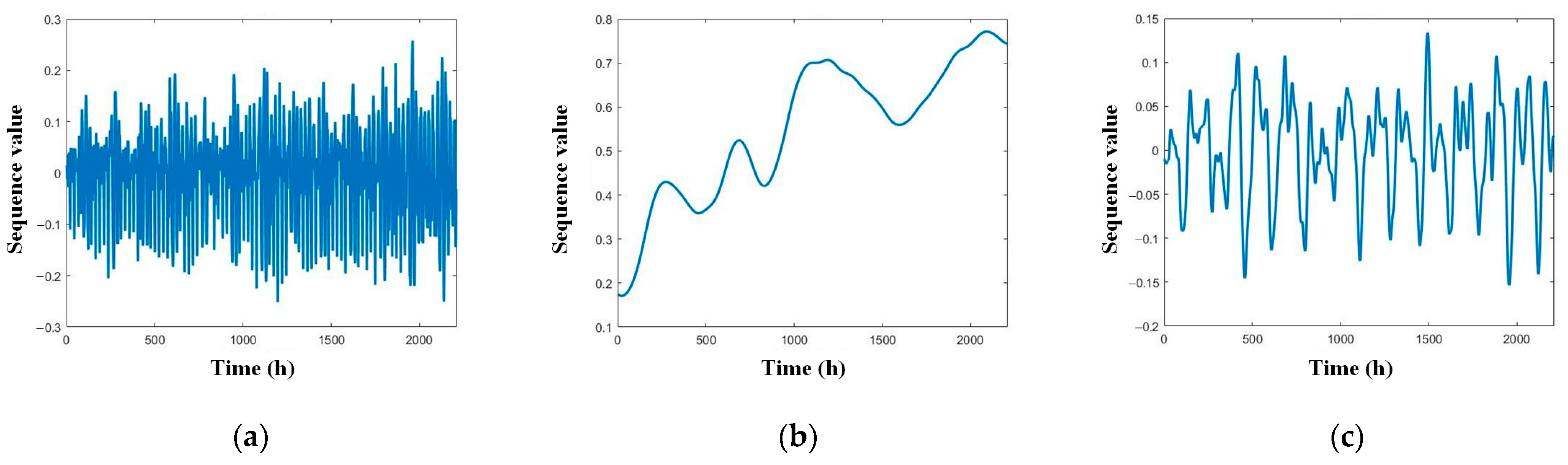
3. Load Feature Extraction Based on Data Decomposition and Clustering

This article proposes a method for extracting load features based on data decomposition and clustering. The method combines the CEEMDAN with the k-medoids clustering based on DTW to construct the feature extraction model, and it plays a pivotal role in mitigating the non-stationarity of load data and decomposing complex load sequences into physically meaningful subsequences, thereby enabling differentiated modeling.

3.1. Theory Related to Data Decomposition

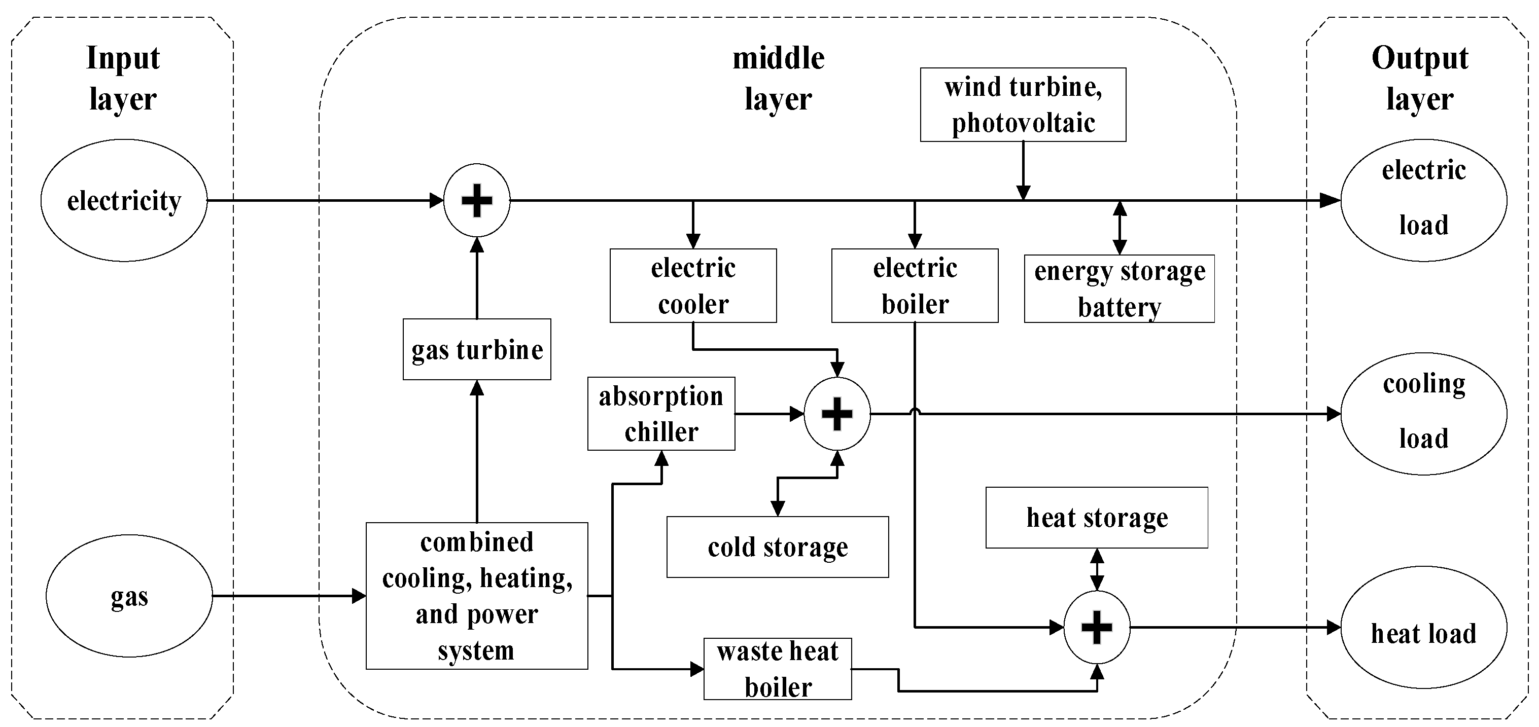
3.1.1. Composition of System Loads

This article divides the system load into four components: typical load component, meteorological sensitive load component, abnormal event load component, and random load component. These categories are based on external factors, such as society, meteorology, and market.

(a) Typical load component: This component is not affected by meteorological factors and shows linear and periodic changes. Its linear variation characterizes the daily average load, while periodic variation is mostly reflected in the point change characteristics over a period of one day or one week. This type of load component reflects the periodicity and multiple coupling of the overall load.

(b) Meteorological sensitive load component: This component is related to meteorological factors, such as temperature, humidity, wind speed, and solar radiation, and is a concentrated reflection of the connection between the overall load and external meteorological factors.

(c) Abnormal event load component: This component is a typical uncertainty component. System failures, related policies, and other abnormal events are important factors that cause the load to deviate significantly from typical load characteristics. This type of load component is a concentrated manifestation of the connection between the overall load and external social and market factors.

(d) Random load components: It is often difficult to obtain the influencing factors associated with this component through simple correlation analysis, and it is generally analyzed through methods such as chaotic time series models and signal decomposition. This type of load component is a concentrated reflection of the randomness of the overall load.

3.1.2. Complete Ensemble Empirical Mode Decomposition with Adaptive Noise

The CEEMDAN algorithm performs time-frequency analysis and processing on nonlinear and non-stationary signals. It also extracts data features and generates a series of intrinsic mode functions with different local features. In integrated energy system load forecasting, it decomposes the load into different load components for targeted analysis and achieves more accurate prediction results. The specific steps of the CEEMDAN algorithm are as follows.

(a) Add white noise ${\epsilon }^m(t)$ to the original load sequence $x(t)$

$$x^m(t)=x(t)+{\epsilon }^m(t),m=1,2,\cdots ,n$$

(5)

In Equation (5), n is the number of times white noise is added.

(b) Perform modal decomposition on $x^m(t)$, obtain several components, and then take the average to obtain the first intrinsic mode function component $IM{F}_1(t)$.

$$IM{F}_1(t)={\displaystyle \frac{1}{n}}{\displaystyle \sum _{i=1}^{n}IM{F}_{ij}(t)}$$

(6)

Subtract $IM{F}_1(t)$ from the original load sequence $x(t)$ to obtain the first remainder.

$$r_1(t)=x(t)-IM{F}_1(t)$$

(7)

(c) Sum $r_1(t)$ and the modal decomposition results of white noise sequence, then perform modal decomposition on the sum results and take the average to obtain $IM{F}_2(t)$.

$$IM{F}_2(t)={\displaystyle \frac{1}{n}}{\displaystyle \sum _{i=1}^{n}EM{D}_1(r_1(t)+EM{D}_1({\epsilon }^i(t)))}$$

(8)

Subtract $IM{F}_2(t)$ from $r_1(t)$ to obtain the second remainder.

$$r_2(t)=r_1(t)-IM{F}_2(t)$$

(9)

(d) Repeat steps (b) and (c) until the remainder cannot be further decomposed, and finally obtain the remainder and each component.

$$r_i(t)=r_{i-1}(t)-IM{F}_i(t)$$

(10)

$$IM{F}_{i+1}(t)={\displaystyle \frac{1}{n}}{\displaystyle \sum _{i=1}^{n}EM{D}_1(r_i(t)+EM{D}_i({\epsilon }^i(t)))}$$

(11)

The obtained remainder and components can be fully reconstructed to obtain the original load data, as shown below.

$$x(t)={\displaystyle \sum _{i=1}^{n}IM{F}_i(t)}+r(t)$$

(12)

3.2. K-Medoids Clustering Based on Dynamic Time Warping

3.2.1. Algorithmic Process

This article proposes a k-medoids clustering algorithm based on dynamic time warping, which is mainly used for correlated load subsequences. This method reduces the random errors introduced by modeling each subsequence in subsequent predictions. The specific steps are as follows. Firstly, set the clustering center by initializing k sample points from the load series. Secondly, based on DTW, allocate each sample point to the nearest clustering center. Thirdly, form a new cluster set and calculate the corresponding new cluster center. Finally, repeat the steps above until the cluster center is fixed.

3.2.2. Evaluation Index of Clustering Algorithm

This article utilizes silhouette coefficients (SC) as the evaluation index, and the formula is shown in Equation (13).

$$SC(i)={\displaystyle \frac{b(i)-a(i)}{\max [a(i),b(i)]}}=\left\{\begin{array}{l}1-{\displaystyle \frac{a(i)}{b(i)}},a(i)<b(i)\\ 0\hspace{1em}\hspace{1em}\hspace{1em},a(i)=b(i)\\ {\displaystyle \frac{a(i)}{b(i)}}-1,a(i)>b(i)\end{array}\right.$$

(13)

In Equation (13), $a(i)$ is the average distance from data $i$ to other data within the class, and $b(i)$ is the average distance from data $i$ to all other types of data. When $SC$ is at a maximum, the clustering effect is the best.

4. Load Forecasting Model

4.1. Load Forecasting Based on Multi-Task Learning

For the problem of multiple load forecasting, it is common practice to convert the loads into multiple individual forecasting problems. However, this method often overlooks the coupling between multiple loads, making it difficult to ensure prediction accuracy. In contrast, if multi-task learning (MTL) is used, it can create a unified training set that facilitates parameter and model space sharing [16].

This article adopts an MTL network based on hard parameter sharing [17]. This allows for sharing the hidden layer of the network across multiple tasks, embedding the data representations of various tasks into the same semantic space to learn common features. The use of hard parameter sharing helps to decrease the risks of overfitting and improve the model’s ability to generalize.

4.2. Deep Learning Theory

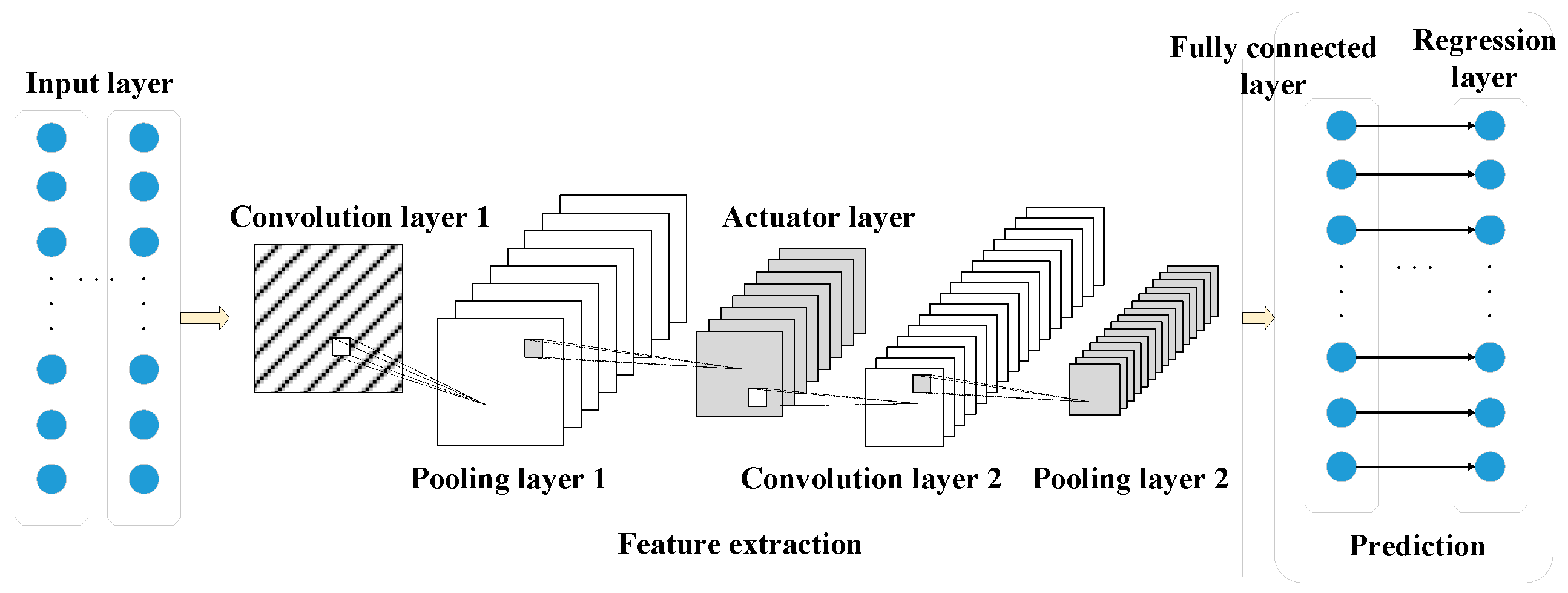
4.2.1. Regression Convolutional Neural Network

A convolutional neural network (CNN) is a type of feedforward neural network that includes convolution calculations. It uses a set of filtering matrices to perform convolution operations on the input raw data and extract data features. The structure of RCNN, which is a CNN used for regression problems, is shown in Figure 2.

Figure 2. Structure of RCNN.

In multiple load forecasting, compared to other neural networks, RCNN can effectively reduce the number of training parameters and network complexity, while possessing strong robustness and high error tolerance.

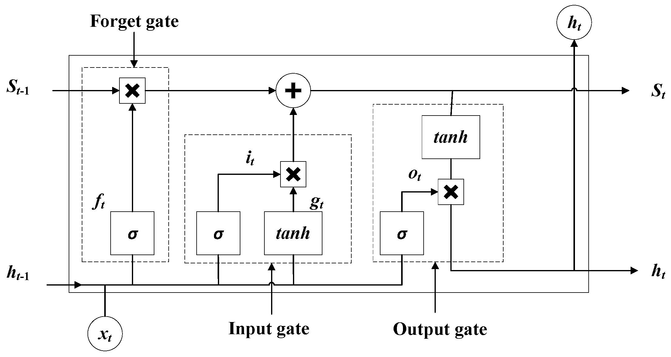
4.2.2. Long Short-Term Memory Network

LSTM is a special type of recurrent neural network (RNN). By employing gated mechanisms and a cell state, LSTM addresses the vanishing gradient problem inherent in traditional RNNs and enables effective modeling of long-term dependencies [18]. The structure of LSTM is shown in Figure 3.

Figure 3. Structure of LSTM.

In multiple load forecasting, compared to other neural networks, LSTM shows excellent performance in learning load series information with long-term dependencies.

4.3. Collaborative Forecasting Model of Multiple Loads

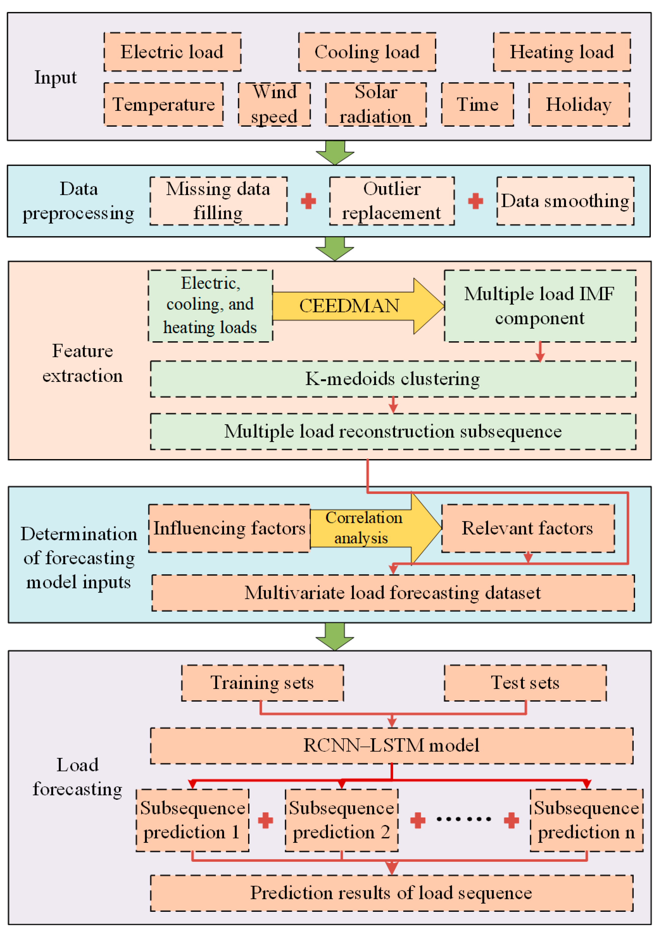
4.3.1. Construction of Forecasting Model

Based on MTL and combining the advantages of RCNN and LSTM, a model combining RCNN and LSTM, known as RCNN–LSTM, was created. The structure of RCNN–LSTM is shown in Figure 4.

Figure 4. Structure of RCNN–LSTM.

To enhance the feature extraction efficiency of RCNN, the structure is optimized. On the basis of the structure shown in Figure 1, an additional convolutional layer and pooling layer are added, and in order to prevent overfitting of the features, random inactivation is used for model optimization. In addition, given LSTM’s superior predictive ability, the fully connected layer and regression layer in RCNN are removed. To improve the prediction accuracy of LSTM, the AdaBelief algorithm [19] is used to optimize the weight update speed of LSTM. This algorithm can achieve relatively fast and stable convergence and ensure the generalization ability of the data.

4.3.2. Evaluation Index

In load forecasting models, the mean absolute percentage error (MAPE) and mean accuracy (MA) are usually used as evaluation indexes. The formulas are as follows.

$$MAPE={\displaystyle \frac{1}{n}}{\displaystyle \sum _{i=1}^n\left|\frac{x(i)-y(i)}{x(i)}\right|\times 100\%}$$

(14)

$$MA=1-MAPE$$

(15)

In Equation (14), $x(i)$ is the i-th actual value and $y(i)$ is the i-th predicted value.

In order to evaluate the overall accuracy of the model, this article introduces the weighted mean accuracy (WMA) based on multiple loads. The formula is as follows.

$$WMA={\alpha }_{1}M{A}_1+\cdot \cdot \cdot +{\alpha }_{k}M{A}_k$$

(16)

In Equation (16), k is the number of load types and ${\alpha }_k$ represents the weight of the load.

In the data sample of this article, the electric and cooling loads are of similar magnitudes, whereas the heat load is one magnitude lower than the electric and cooling loads. Consequently, the weights for cold, heat, and electric loads are set to 0.4, 0.4, and 0.2, respectively [20].

4.3.3. Forecasting Process

The overall framework of the collaborative forecasting method of multiple loads in an integrated energy system based on feature extraction and deep learning proposed in this article is shown in Figure 5.

Figure 5. General framework of the forecasting model.

The specific process is as follows.

(a) Data preprocessing: Fill missing data, replace outliers, and smooth data for load data.

(b) Feature extraction for multiple load: Use CEEMDAN to decompose the multiple load series and obtain IMFs. Then, k-medoids clustering based on DTW is used to cluster the IMFs, resulting in reconstruction subsequences.

(c) Determine prediction model inputs: Firstly, the data must be normalized. Then, distinguish the types of influencing factors. Use the Pearson correlation coefficient to calculate the correlation between multiple loads, and GRA to calculate the correlation between loads and external factors. Finally, select influencing factors with correlation coefficients greater than 0.4, and load reconstruction subsequences as inputs for the prediction model.

(d) Load forecasting: Firstly, set the parameters of RCNN. The input of RCNN is the influencing factors obtained through correlation analysis, and its output, along with the load reconstruction subsequence, is used as the input to LSTM. Then, set the parameters of LSTM. Perform multi-task forecasting on the reconstruction subsequences of multiple loads and obtain the results.

5. Case Study

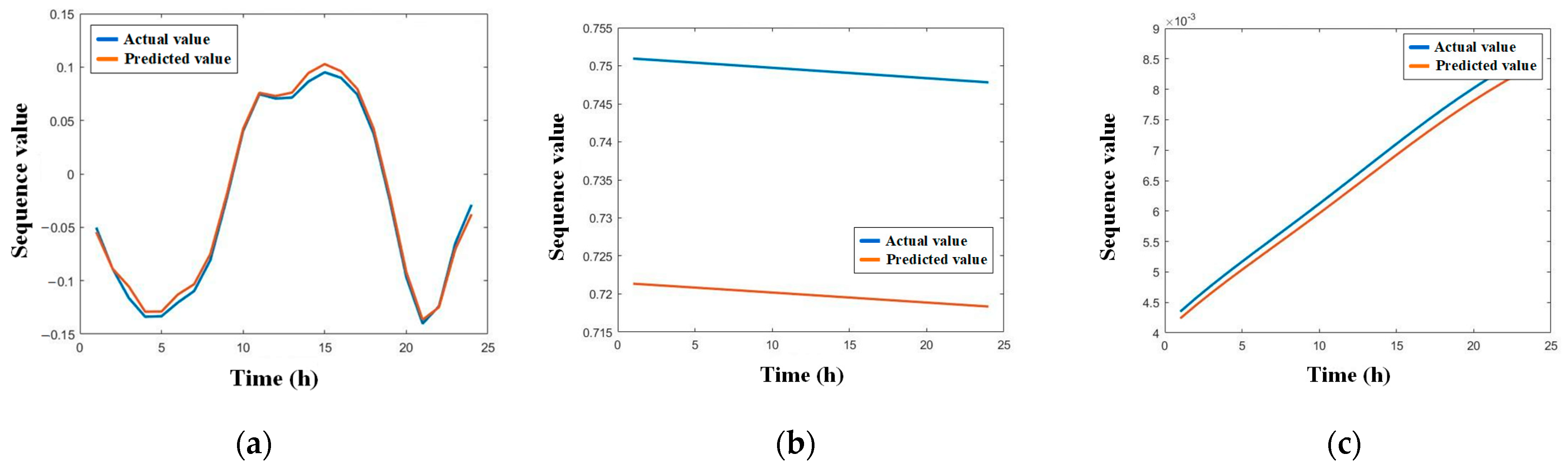
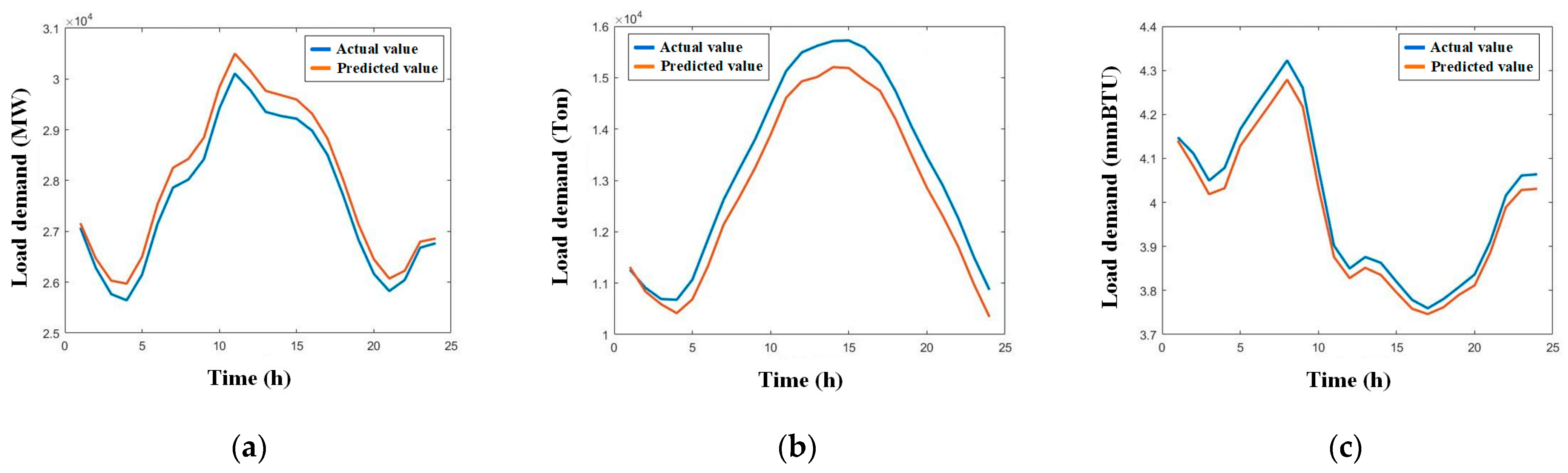
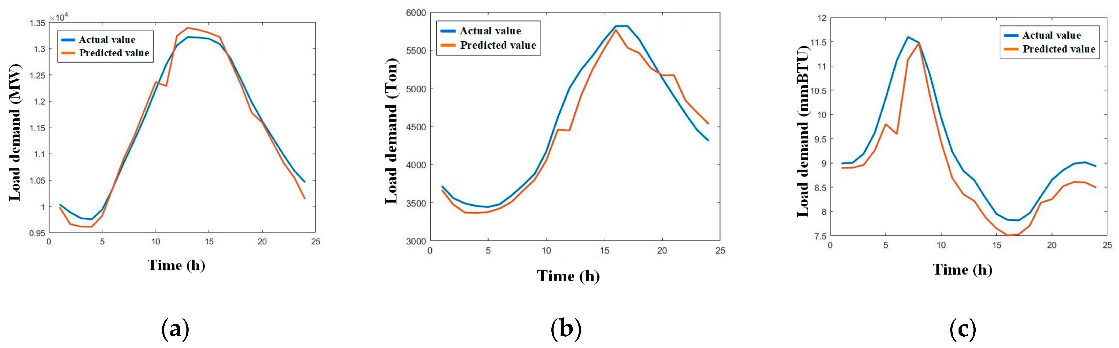
5.1. Prediction Example

The multiple load data used in this article are from the Tempe campus of Arizona State University, and the meteorological data are from the National Renewable Energy Laboratory in the United States [21].

Cooling, heating, and electric load data from June 2022 to August 2022 and December 2022 to February 2023, as well as data on factors such as temperature and wind speed were selected as training samples, with a sampling interval of 1 h. The corresponding data of a typical summer working day on 5 August, a summer rest day on 6 August, a winter working day on 27 January, and a winter rest day on 28 January were selected as the test samples.

RCNN adopts a convolutional neural network model with a convolution kernel size of 3, a sliding step size of 1, three convolution layers, and three downsampling layers. A moderate convolution kernel size can effectively capture local features of data, a small stride ensures the continuity and fineness of feature extraction, and a three-layer structure of convolution and downsampling balances the complexity and generalization ability of the model. Additionally, one hidden layer was implemented for LSTM, and gradient training was performed employing the AdaBelief algorithm. Training proceeded for a maximum of 100 iterations at an initial learning rate of 0.001. The decay rates for estimating first-order moments and second-order moments are 0.99 and 0.999, respectively.

After data preprocessing, CEEMDAN was used to decompose the load series. The parameters were set as a signal-to-noise ratio of 0.2, number of noise additions of 100, and maximum number of iterations of 100. Taking the summer electric load data as an example, the results of the data decomposition are shown in Figure 6.

Figure 6. Decomposition results of summer electric load.

After completing data decomposition, the k-medoids algorithm was used based on DTW to cluster the IMFs. Through comprehensive analysis of clustering evaluation indicators, the optimal number of clusters k was determined to be 3. Table 1 shows the composition of each reconstruction subsequence.

Table 1. Components of the reconstruction subsequence of electric load.

Load Series	Composition of Reconstruction Subsequence
C1	IMF1, IMF2, IMF3, IMF4
C2	IMF9, IMF10, IMF11, RES
C3	IMF5, IMF6, IMF7, IMF8

The summer electric load reconstruction subsequence is shown in Figure 7.

Figure 7. Reconstruction subsequence of summer electric load. (a) C1; (b) C2; (c) C3.

According to the system load composition proposed in this article, in the reconstruction subsequence of summer electric load, C1 is a high-frequency component with no significant change pattern, corresponding to the random load component. C2 exhibits the characteristic of trend changes, corresponding to the meteorological sensitive load component and the abnormal event load component. C3 has a certain periodicity, corresponding to the typical load component.

After obtaining the reconstruction subsequence, a correlation analysis was performed on its influencing factors to identify those with high correlation. Table 2 shows the correlation coefficients between each reconstruction subsequence and its influencing factors, using the summer electric load subsequence as an example.

Table 2. Correlation coefficients between summer electric load reconstruction sequences and influencing factors.

Load Series	Cooling Load	Heating Load	Wind Speed	Solar Radiation	Temp	Time	Holiday
C1	0.760	0.340	0.356	0.333	0.376	0.233	0.333
C2	0.785	0.413	0.446	0.648	0.689	0.656	0.569
C3	0.816	0.372	0.340	0.334	0.303	0.434	0.334

The influencing factors with correlation coefficients greater than 0.4 were selected as inputs to the prediction model, and they are shown in Table 3.

Table 3. Influencing factors corresponding to each reconstruction subsequence.

Load Series	Influencing Factor
C1	Cooling load
C2	Cooling load, heating load, wind speed, solar radiation, temp, time, holiday
C3	Cooling load, time

5.2. Analysis of Results

After completing the model training, the actual load data were selected as the test set. Taking typical summer days as an example, the load reconstruction subsequence and related influencing factors were input into the prediction model to obtain multivariate load prediction results. The reconstruction subsequence prediction results of a summer work day are shown in Figure 8.

Figure 8. Results of reconstruction subsequence prediction of summer working day electric loads. (a) Reconstruction subsequence 1; (b) reconstruction subsequence 2; (c) reconstruction subsequence 3.

After superimposing the prediction results of each reconstruction subsequence, inverse normalization was performed to obtain the load forecasting results. The multiple-load forecasting results for summer working days and rest days are shown in Figure 9 and Figure 10, respectively.

Figure 9. Multiple load forecasting results for summer working day. (a) Electric load; (b) cooling load; (c) heating load.

Figure 10. Multiple load forecasting results for summer rest day. (a) Electric load; (b) cooling load; (c) heating load.

The evaluation indexes are shown in Table 4.

Table 4. Evaluation indexes for prediction results in summer working day and rest day.

Season	Date Type	Load Type	MAPE/%	MA/%	WMA/%
Summer	Working day	Cooling	2.24	97.76	97.67
		Heating	2.75	97.25
		Electric	1.69	98.31
	Rest day	Cooling	2.40	97.60	97.32
		Heating	3.21	96.79
		Electric	2.16	97.84

Table 4 shows that the model has high prediction accuracy for multiple summer loads under different day types. However, the prediction accuracy for electric and cooling loads is lower than that for heating loads. This is due to the strong coupling between electric and cooling loads in summer. During summer, electric loads are affected by the fluctuation of cooling loads. On the other hand, the heating load is relatively stable, so its prediction accuracy is the highest.

The multiple-load forecasting results for winter working days and rest days are shown in Figure 11 and Figure 12, respectively.

Figure 11. Multiple load forecasting results for winter working day. (a) Electric load; (b) cooling load; (c) heating load.

Figure 12. Multiple load forecasting results for winter rest day. (a) Electric load; (b) cooling load; (c) heating load.

The evaluation indexes are shown in Table 5.

Table 5. Evaluation indexes for prediction results in winter working day and rest day.

Season	Date Type	Load Type	MAPE/%	MA/%	WMA/%
Winter	Working day	Cooling	2.92	97.08	97.60
		Heating	1.66	98.34
		Electric	2.87	97.13
	Rest day	Cooling	2.08	97.92	97.79
		Heating	1.88	98.12
		Electric	3.12	96.88

Table 5 shows that the winter model prediction results are similar to those of the summer. The model has high prediction accuracy for multiple winter loads under different day types, but the accuracy is lower for electric and heating loads compared to cooling loads. This is due to the strong coupling between electric and heating loads in winter. During winter, the electric load is affected by the fluctuation of the heating load. On the other hand, the cooling load is relatively stable in winter, resulting in higher prediction accuracy.

To verify the effectiveness of the model described in this article, it was compared to scenarios where cooling, heating, and electric loads were predicted separately, as well as a scenario where load forecasting was performed without data decomposition and clustering reconstruction. The results are presented in Table 6.

Table 6. Results of each prediction scenario.

Season	Date Type	Load Type	MAPE/%
			Proposed Model	Scenario 1	Scenario 2
Summer	Working day	Cooling	2.2420	9.3546	4.6862
		Heating	2.7489	7.6739	4.2642
		Electric	1.6882	9.6367	5.1323
	Rest day	Cooling	2.4010	9.5923	5.5553
		Heating	3.2114	8.6851	4.6650
		Electric	2.1628	9.2516	4.9009
Winter	Working day	Cooling	2.9202	9.3546	3.4080
		Heating	1.6633	7.6739	3.6309
		Electric	2.8721	9.6367	5.7045
	Rest day	Cooling	2.0787	8.5504	4.7295
		Heating	1.8837	7.8862	5.0586
		Electric	3.1156	8.7932	4.6766

From Table 6, it can be seen that compared with load forecasting scenarios where cooling, heating, and electric loads are predicted separately and without data decomposition and clustering reconstruction, the model proposed in this article has higher prediction accuracy. This indicates that the quantitative analysis steps of the correlation between multiple loads and the load feature extraction steps based on data decomposition and clustering reconstruction can both reduce the error of load forecasting and improve the prediction accuracy.

To verify the feasibility and effectiveness of the proposed model, a comparison was conducted between it and the models referenced in [12,22,23,24]. The results are presented in Table 7.

Table 7. Comparison results of different prediction models.

Index	Proposed Model	WPD–RNN [12]	RCNN–SVR [22]	GRU–ELM [23]	ARIMA [24]
WMA/%	97.342	95.678	96.750	94.262	72.593

To verify the adaptability of the model proposed in this article to multi-task learning, a comparison was made between the model proposed in this paper and the models proposed in [25,26] using a multi-task learning mechanism. The results are shown in Table 8.

Table 8. Comparison results of different multi-task learning prediction models.

Index	Proposed Model	IGTCN–GRU [25]	MMoE–LSTM [26]
WMA/%	97.342	97.063	96.160

In summary, the model in this article is feasible and efficient and can effectively improve the accuracy of load prediction.

6. Conclusions

This article proposes a collaborative forecasting method of multiple loads in an integrated energy system based on feature extraction and deep learning. The main contributions are summarized as follows. Firstly, a load feature extraction method based on data decomposition and clustering is proposed. This method uses CEEMDAN for load data decomposition and uses the k-medoids clustering based on DTW to cluster IMFs into reconstruction subsequences. The results of the example show that this method can effectively improve prediction accuracy. Secondly, a correlation analysis method for load-influencing factors is proposed. To achieve this, the Pearson correlation coefficient and GRA were applied to examine the linear and non-linear relationships among the data. This methodology aims to quantify the correlation between different factors and loads. The results of this study demonstrate the method’s effectiveness in enhancing load forecasting outcomes. Finally, a prediction model for collaborative load forecasting that employs RCNN–LSTM and MTL is proposed. Influencing factors are extracted using RCNN for feature extraction, and LSTM is selected as the prediction model. MTL is used to output the predicted values for each load reconstruction subsequence, which is then integrated to produce the final results. The results of practical examples indicate that MTL is effective, and the model demonstrates high accuracy when forecasting multiple loads in integrated energy systems. Future research may consider adopting more advanced deep learning models and exploring other methods that can achieve feature extraction, with a view to further improve the efficiency and accuracy of load forecasting in integrated energy systems.

References

- Yu, X.D.; Xv, X.D. A Brief Review to Integrated Energy System and Energy Internet. Trans. China Electrotech. Soc. 2016, 31, 1–13. [Google Scholar]
- Sun, D.; Liu, Z.; Shao, J.; Lin, Z. Review on low carbon planning and operation of integrated energy systems. Energy Sci. Eng. 2022, 10, 3201–3215. [Google Scholar] [CrossRef]
- Zhu, J.; Dong, H.; Zheng, W.; Li, S.; Huang, Y.; Xi, L. Review and prospect of data-driven techniques for load forecasting in integrated energy systems. Appl. Energy 2022, 321, 119269. [Google Scholar] [CrossRef]
- Ding, N.; Benoit, C.; Foggia, G.; Besanger, Y.; Wurtz, F. Neural network-based model design for short-term load forecast in distribution systems. IEEE Trans. Power Syst. 2016, 31, 72–81. [Google Scholar] [CrossRef]
- Cheng, H.; Hu, X.; Wang, L.; Liu, Y.; Yu, Q. Review on research of regional integrated energy system planning. Autom. Electr. Power Syst. 2019, 43, 2–13. [Google Scholar]
- Zhou, N.; Liao, J.; Wang, Q.; Li, C.; Li, J. Analysis and prospect of deep learning application in smart grid. Autom. Electr. Power Syst. 2019, 43, 180–191. [Google Scholar]
- Chen, H.; Wang, J.; Tang, B.; Xiao, K.; Li, J. An integrated approach to planetary gearbox fault diagnosis using deep belief networks. Meas. Sci. Technol. 2017, 28, 180–191. [Google Scholar] [CrossRef]
- Deng, D.Y.; Li, J.; Teng, Y.; Huang, Q. Short-term electric load forecasting based on EEMD-GRU-MLR. Power Syst. Technol. 2020, 44, 593–602. [Google Scholar]
- Zhang, Y.M.; Sun, M.; Ji, X.Q. Short-term load forecasting of integrated energy system based on modal decomposition and multi-task learning model. High Volt. Eng. 2025, 51, 1–18. [Google Scholar]
- Zhu, J.; Dong, H.; Li, S.; Chen, Z.; Luo, T. Review of Data-driven Load Forecasting for Integrated Energy System. Proc. Chin. Soc. Electr. Eng. 2021, 41, 7905–7924. [Google Scholar]
- Shi, J.Q.; Tan, T.; Guo, J. Multi-Task Learning Based on Deep Architecture for Various Types of Load Forecasting in Regional Energy System Integration. Power Syst. Technol. 2018, 42, 698–707. [Google Scholar]
- Luo, F.; Zhang, X.; Yang, X.; Yao, Z.; Zhu, L.; Qian, M. Load analysis and prediction of integrated energy distribution system based on deep learning. High Volt. Eng. 2021, 47, 23–32. [Google Scholar]
- Xiao, Y.; Zhao, Y.; Tu, Z.; Qian, B.; Chang, R. Topology checking method for low voltage distribution network based on improved Pearson correlation coefficient. Power Syst. Prot. Control. 2019, 47, 37–43. [Google Scholar]
- Zhao, H.L.; Zhang, D.D.; Huang, S.; Mo, S.; Wei, H. Analysis on the Relation Between Cloud-to-ground Lightning Density and Lightning Trip Rate in Hainan Province Based on Pearson Correlation Coefficient. High Volt. Appar. 2019, 55, 186–192. [Google Scholar]
- Yang, N.; Li, H.; Yuan, J.; Li, S.; Wang, X. Medium-and long-term load forecasting method considering grey correlation degree analysis. Proc. CSU-EPSA 2018, 30, 108–114. [Google Scholar]
- Aguiar-Pérez, J.M.; Pérez-Juárez, M.Á. An Insight of Deep Learning Based Demand Forecasting in Smart Grids. Sensors 2023, 23, 1467. [Google Scholar] [CrossRef] [PubMed]
- Lu, Z.; Jie, G.; Lu, M. Short-term load forecasting for integrated energy system based on coupling features and multi-task learning. Autom. Electr. Power Syst. 2022, 46, 58–66. [Google Scholar]
- Cho, K.; Van Merriënboer, B.; Gulcehre, C.; Bahdanau, D.; Bougares, F.; Schwenk, H.; Bengio, Y. Learning Phrase Representations using RNN Encoder-Decoder for Statistical Machine Translation. arXiv 2014, arXiv:1406.1078. [Google Scholar]
- Zhuang, J.; Tang, T.; Ding, Y.; Tatikonda, S.C.; Dvornek, N.; Papademetris, X.; Duncan, J. AdaBelief optimizer: Adapting stepsizes by the belief in observed gradients. In Proceedings of the Neural Information Processing Systems (NeurIPS), Virtual, 6–12 December 2020; Volume 33. [Google Scholar]
- Li, R.; Sun, F.; Ding, X.; Han, Y.; Liu, Y.P.; Yan, J.R. Ultra short-term load forecasting for user-level integrated energy system considering multi-energy spatio-temporal coupling. Power Syst. Technol. 2020, 44, 4121–4131. [Google Scholar]
- Ye, J.H.; Cao, J.; Yang, L.; Luo, F.Z. Ultra short-term load forecasting of user level integrated energy system based on variational mode decomposition and multi-model fusion. Power Syst. Technol. 2022, 46, 2610–2622. [Google Scholar]
- Zhu, L.; Wang, X.; Ma, J.; Chen, Q.; Qi, X. Short-term load forecast of integrated energy system based on wavelet packet decomposition and recurrent neural network. Electr. Power Constr. 2020, 41, 131–138. [Google Scholar]
- Sun, X.; Li, J.; Zeng, B.; Gong, D.; Lian, Z. Small-sample day-ahead power load forecasting of integrated energy system based on feature transfer learning. IET Control Theory A 2021, 38, 63–72. [Google Scholar]
- Li, N.; Jiang, Y.; Huang, S.; Mao, L. Short-Term Load Forecasting Based on ARIMA Transfer Function Model. Power Syst. Technol. 2009, 33, 93–97+103. [Google Scholar]
- Tan, M.; Hu, C.; Chen, J.; Wang, L.; Li, Z. Multi-node load forecasting based on multi-task learning with modal feature extraction. Eng. Appl. Artif. Intel. 2022, 112, 104856. [Google Scholar] [CrossRef]
- Wu, C.; Yao, J.; Xue, G.; Wang, J.; Wu, Y.; He, K. Load forecasting of integrated energy system based on MMoE multi-task learning and LSTM. Electr. Power Autom. Equip. 2022, 42, 33–39. [Google Scholar]
Disclaimer/Publisher’s Note: The statements, opinions and data contained in all publications are solely those of the individual author(s) and contributor(s) and not of MDPI and/or the editor(s). MDPI and/or the editor(s) disclaim responsibility for any injury to people or property resulting from any ideas, methods, instructions or products referred to in the content. |
© 2025 by the authors. Licensee MDPI, Basel, Switzerland. This article is an open access article distributed under the terms and conditions of the Creative Commons Attribution (CC BY) license (https://creativecommons.org/licenses/by/4.0/).