Abstract
Energy efficiency in road lighting is increasingly critical for sustainable urban development, yet numerical indicators essential for objective evaluation are often misunderstood or misapplied. This paper addresses fundamental misconceptions in interpreting the Power Density Indicator (PDI), a key metric for assessing lighting system efficiency. Through analysis of Romanian street lighting modernization projects and extensive literature review, we demonstrate widespread misunderstanding of PDI’s properties, including inappropriate summation across streets and failure to recognize its independence from road class. We present a comprehensive methodology for PDI interpretation and optimization through spatial visualization of Luminous Intensity Distribution Curves (LIDCs) using MATLAB’s MESH function. The theoretical framework derives minimum achievable PDI values as a function of LED-specific efficacy and system utilance. Case studies from 181 streets in Romanian cities reveal significant optimization potential. Finally, we demonstrate, through computational simulation, the theoretical ideal: a perfectly adapted LIDC achieving unitary utilance, confirming that minimum PDI depends solely on LED efficacy and optical efficiency. These findings provide practical guidance for designers to optimize energy efficiency while meeting photometric requirements.
1. Introduction
The transition to LED technology in road lighting presents unprecedented opportunities for energy efficiency and sustainable development. However, technological advancement alone does not guarantee optimal outcomes. The proper use of standardized numerical indicators is essential for objective evaluation, comparison, and optimization of lighting installations.
EN 13201-5 [1] introduced numerical indicators for road lighting energy performance, analogous to the Lighting Energy Numerical Index (LENI) established by EN 15193 in 2007 for building lighting [2]. These indicators—particularly the Power Density Indicator (PDI, denoted Dp) and Annual Energy Consumption Indicator (AECI, denoted DE)—were developed to enable meaningful comparisons and classifications. Despite their standardization, these indicators are frequently omitted from energy efficiency studies or applied incorrectly, undermining the goal of sustainable lighting design.
This paper originated from observations during extensive street lighting modernization tenders in Romania, where the Ministry of Environment mandated PDI calculations that violated fundamental properties of the indicator. Specifically, projects were required to calculate PDI for entire localities by summing PDI values across individual streets—a mathematical impossibility since PDI is an intensive property, not an extensive one. This fundamental misunderstanding prompted a systematic investigation of how PDI and related indicators are interpreted in practice.
Through literature review, we identified a pattern of similar misconceptions across published research. Some studies present energy efficiency improvements without any numerical indicators [3,4,5]. Others use indicators but with critical ambiguities that prevent meaningful comparison [6,7,8]. Even papers specifically focused on PDI demonstrate incomplete understanding of its relationship with system design parameters [9,10,11,12,13]. Most significantly, the influence of Luminous Intensity Distribution Curves (LIDCs) on energy efficiency is rarely considered systematically.
This paper addresses these gaps through three contributions: (1) clarification of PDI interpretation and its independence from geometric factors, (2) development of visualization methods to understand complete spatial LIDC characteristics beyond traditional meridian planes, and (3) derivation of theoretical minimum PDI values achievable with optimized luminaire design. We demonstrate these concepts through case studies of Romanian street lighting projects and computational validation using DIALux EVO 13.1 simulations.
2. Literature Review
The literature reveals three categories of issues in applying energy efficiency indicators to road lighting: complete absence of numerical metrics, use of indicators with insufficient detail for comparison, and fundamental misunderstanding of indicator properties.
2.1. Absence of Standardized Numerical Indicators
Multiple studies present street lighting modernization under the imperative of energy efficiency while omitting quantitative metrics entirely. Zdunic [3] discusses avoiding oversizing based on the outdated belief that “more light is better” but provides no energy density values. Similarly, Omran et al. [4] report absolute energy consumption reductions without normalizing by illuminated area or illuminance level, despite EN 15193 having established such indicators for interior lighting by 2007 [2].
Anthopoulou and Doulos [5] present a case study of the Egnatia Odos highway lighting upgrade. Although EN 13201-5 appears in their bibliography, they report only global energy savings without calculating PDI or AECI. This pattern—citing relevant standards without applying their quantitative framework—appears repeatedly in the literature.
The absence of standardized indicators prevents objective assessment of whether claimed efficiency improvements represent genuine optimization or merely fortuitous energy reduction accompanying LED adoption. Without normalized metrics, it is impossible to distinguish a well-designed efficient system from an inefficient LED installation that happens to consume less energy than the high-pressure sodium system it replaced.
2.2. Incomplete or Ambiguous Application of Indicators
A second category of papers uses energy metrics but with insufficient specificity for meaningful interpretation. Dimitrakis et al. [6] compare LED, high-pressure sodium (HPS), and metal halide lamp (MHL) technologies, citing EN 13201 but omitting Part 5. They express energy efficiency in kW/km without specifying road width or class, making comparisons impossible. Ciobanu and Pentiuc [7] exhibit the same pattern: citing EN 13201 while omitting Part 5 and its quantitative framework.
Panchev [8] calculates PDI = 0.021 W/(lx·m2) but discusses the value primarily in terms of street cross-section rather than recognizing PDI’s normalization properties. The paper reports AECI = 2.67 kWh/m2 versus EN 13201-5’s reference value of 2.4–2.5 kWh/m2 for class M2, but does not explain the discrepancy. Notably, if we reverse-calculate PDI from their AECI using Equation (1) with and Eav = 30 lx:
2.3. Fundamental Misunderstanding of PDI Properties
The most concerning issues involve papers specifically addressing PDI but demonstrating incomplete understanding of its fundamental characteristics. Gasparovsky [11] states that “mounting height and arm length affect the indicators only indirectly.” This reveals a critical misunderstanding: for a given luminaire, changing mounting height and arm length fundamentally alters utilance (the ratio of flux received by the street surface to flux emitted by the lamp), which directly determines PDI. There is nothing indirect about this relationship.
The same author [11] analyzes PDI values for road classes M3 and M5 without recognizing that PDI must be identical for both classes when properly calculated. Since PDI is normalized by average illuminance Eaverage, the road class cancels out. Furthermore, Ref. [11] shows PDI increasing for streets narrower than 7 m—a pattern left unexplained despite its clear indication of decreasing utilance in narrow geometries.
Gasparovsky and Dubnicka [12] assert: “If the required lighting class changes during the night and/or through the seasons… the PDI should be calculated separately for each lighting class.” This is fundamentally incorrect. Dimming reduces both average illumination and effective power consumption proportionally, leaving PDI unchanged. This misconception may stem from early LED dimming technology (circa 2014) when 50% illumination reduction achieved only 30% power reduction, but modern LED dimming maintains constant PDI across dimming levels.
In a more recent work, Gasparovsky et al. [13] seek typical PDI values and recognize LED efficacy’s importance (noting EN 13201-5 values were obtained with 100–105 lm/W LEDs). However, they analyze PDI across road classes M1-M6 without noticing that these values should be equal. They also examine PDI “variation” alongside AECI, though AECI obviously increases several-fold from M6 to M1 while PDI should remain constant. Most significantly, they do not consider how LIDC characteristics influence achievable PDI values, nor do they observe that PDI decreases with increasing illuminated surface area (higher utilance) when sidewalks are included.
Aghemo et al. [9] present data showing PDI varying between 10 and 55 mW/(lx·m2), with pedestrian areas reaching 20–175 mW/(lx·m2). They note this pattern but do not explain it. The high PDI in narrow pedestrian alleys results from low utilance—much of the luminous flux necessarily illuminates adjacent areas for adequate surrounding ratio, reducing the fraction reaching the designated surface.
Tomczuk et al. [14] base their PDI analysis on measurements rather than calculations, which should provide higher-confidence results. However, they report extreme values (6, 8, 10, 56, 64, 66 mW/(lx·m2)) without interpreting this wide range. The order-of-magnitude variation suggests fundamentally different installation efficiencies that merit systematic investigation.
These patterns reveal incomplete understanding of PDI’s fundamental properties: it is intensive (not additive), independent of road class (when properly normalized), constant across dimming levels (with modern LEDs), and directly dependent on utilance. Most importantly, the literature rarely connects PDI systematically to the spatial characteristics of LIDC that determine utilance.
2.4. The Missing Link: Luminous Intensity Distribution Curves
When energy efficiency [15] is discussed, LED specific efficacy (lm/W) receives appropriate attention, but the crucial role of luminous intensity distribution is systematically neglected [16]. This gap is particularly striking given that LIDC characteristics directly determine utilance and therefore PDI.
Bayer et al. [17] apply genetic algorithms to optimize road lighting design, but their geometry (3 m road width, 40 m pole spacing) creates unacceptable longitudinal illuminance variation despite nearly uniform transverse distribution. They miss the fundamental problem: finding LIDC that creates uniform illumination across the entire road surface. While constant illumination would not produce constant luminance (due to non-diffuse asphalt reflection), this theoretical ideal reveals how optimal LIDC should be structured.
Tomczuk et al. [14] discuss pedestrian crossing illumination but inadequately emphasize the importance of LIDC. Their Figure 8 shows a conventional distribution without explaining its suitability (or lack thereof) for maximizing vertical illuminance at pedestrian crossings. A sideways-directed distribution would better achieve this goal, yet the connection between specific LIDC characteristics and vertical illumination optimization remains unexplored.
Wannapasert et al. [18] evaluate LED luminaires for two-lane roadways in 2024, still focusing primarily on HPS-to-LED conversion. Although they cite EN 13201, PDI is not discussed. More critically, luminaire variants are described only by nominal power (60 W to 140 W) with no LIDC information—the very parameter that determines whether a given power level represents efficient or wasteful design.
Zseller and Samu [19] explicitly address LIDC optimization, seeking “arbitrary luminous intensity distribution” through metaheuristic algorithms. They define a merit function (their Equation (3)) for optimization, but despite citing EN 13201, they omit the PDI criterion. More fundamentally, they pursue computational optimization without performing the simpler reverse calculation: given required road luminance distribution, what LIDC is necessary? This direct geometric approach provides physical insight that purely algorithmic optimization may miss.
The incomplete treatment of LIDC in the literature motivated our approach: systematic visualization of complete spatial LIDC characteristics (not merely two meridian planes), reverse calculation of ideal distributions for specified illumination patterns, and explicit connection between LIDC properties and achievable PDI values through the utilance relationship.
3. Methodology
This research employs three complementary approaches: theoretical analysis, computational visualization, and simulation-based validation. Each method addresses specific aspects of PDI optimization and LIDC characterization.
3.1. LIDC Analysis and Visualization
We derive minimum achievable PDI values through systematic analysis of EN 13201-5 equation structure, progressively decomposing the PDI expression to reveal its dependence on fundamental system parameters: LED specific efficacy, luminaire optical efficiency, and system utilance. This decomposition exposes the theoretical limits of PDI optimization and identifies which parameters designers can control.
Conventional LIDC representation shows only C0–C180° and C90–C270° meridian planes, where C is photometric azimuth. This two-dimensional representation is fundamentally insufficient for understanding spatial flux distribution. We developed MATLAB-R2024b based three-dimensional visualization using MESH functions applied to luminous intensity vectors in spherical coordinates. LDT and IES file formats were parsed to extract complete angular distribution data, which was then transformed for spatial rendering.
The MESH representation treats luminous intensity magnitudes at each angular position as vertices of a three-dimensional surface. This geometric locus of LIDC vector endpoints reveals flux distribution characteristics invisible in conventional two-plane projections, particularly the diagonal concentration of flux that critically affects utilance.
3.2. Ideal LIDC Calculation
To establish optimization targets, we computed ideal LIDC through reverse photometric calculation. For specified constant illumination levels on roadway (20 lx) and sidewalk (10 lx), we determined the required luminous intensity at each angular position. This inverse problem was solved in MATLAB using geometric relationships between source position, target points, and photometric fundamentals.
The calculated ideal distribution serves two purposes: (1) it demonstrates the theoretical utilance limit of unity, and (2) it provides a quantitative target for evaluating real luminaire performance. The resulting LDT file was visualized using both SCATTER3 and MESH functions to reveal the required spatial flux distribution characteristics.
3.3. Case Study Analysis
PDI values from actual street lighting modernization projects in Satu Mare (114 streets) and Iasi (67 streets) were extracted from DIALux calculations. These values were ordered and plotted to reveal patterns in design quality and identify outliers requiring design revision. This approach provides practical validation of whether current design practices achieve near-optimal efficiency or leave substantial room for improvement.
3.4. Computational Validation
The ideal LIDC was imported into DIALux EVO and simulated for a representative street geometry (7 m width, 40 m pole spacing, 12 m mounting height, −1 m overhang). Simulation results validate both the unity utilance achievement and the minimum PDI calculation. The isolux curves and numerical results (average illuminance, uniformity, threshold increment, PDI) were extracted to confirm theoretical predictions.
4. Theoretical Framework: Minimum Achievable PDI
The Power Density Indicator quantifies energy efficiency independent of road geometry or lighting class. Understanding its theoretical minimum requires systematic decomposition of its defining equation from EN 13201-5.
4.1. PDI Definition and Decomposition
EN 13201-5 defines PDI as the ratio of total power to total luminous flux on the calculation surface (Equation (2)):
where Pi represents individual luminaire power, Ei represents illuminance at point i, and Ai represents area of element i. The denominator constitutes the useful flux emitted by luminaire:
The useful luminous flux is the fraction of total luminaire flux emitted by a luminaire that reaches the working plane, expressed through utilance U (a dimensionless coefficient less than unity):
The total luminaire flux results from LED flux Φ multiplied by optical efficiency of the luminaire :
We recognize the LED specific efficiency expressed in lm/W:
4.2. Minimum PDI and Design Implications
For an ideal installation where utilance U approaches unity (all emitted flux reaches the target surface), PDI achieves its minimum value:
This expression reveals several critical insights:
- PDI has a technological minimum value which we must aim for in the design process.
- For given LED and optical efficiencies, PDI optimization reduces to maximizing utilance through optimal LIDC design.
- Minimum PDI provides a reference value for evaluating any actual installation; actual PDI/minimum PDI quantifies how far a design is from theoretical optimum.
- Different street geometries can achieve the same minimum PDI if utilance is optimized through appropriate LIDC selection.
Consider a practical example: for = 125 lm/W and R_LO = 90%, it will result PDImin = 8.8 mW/(lx·m2).
5. Advanced Visualization of Luminous Intensity Distribution
Comprehensive understanding of LIDC requires moving beyond conventional two-plane representation to full spatial visualization. This section presents progressive refinement of visualization methods, revealing flux distribution characteristics essential for utilance optimization.
5.1. Limitations of Conventional Representation
Figure 1 shows a typical LIDC visualization from LDT Editor (DIAL), presenting only C0–C180 (longitudinal) and C90–C270 (transverse) meridian planes. This representation is fundamentally insufficient. Figure 2 demonstrates this limitation by adding the C45–C225 (diagonal) plane, which exhibits significantly higher luminous intensity than the values visible in the two conventional planes.
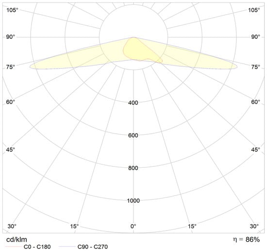
Figure 1.
Typical example luminous intensity curves for street lighting luminaire, obtained by LDT Editor by DIAL.
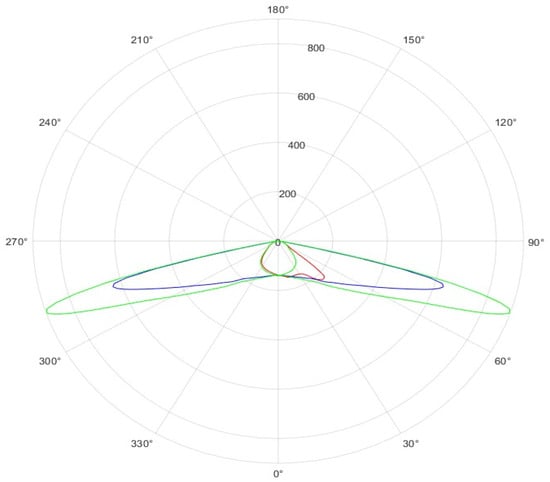
Figure 2.
LIDC from Figure 1, with an additional plane C45–C225 (green), plane C0–C180 (red), plane C90–C270 (blue) obtained in MATLAB from reading an LDT file (cd/klm).
This diagonal concentration of flux critically affects how luminaires perform in actual installations, yet it remains invisible in standard representations. Without understanding complete spatial distribution, designers cannot reliably predict system utilance or optimize PDI.
5.2. Three-Dimensional MESH Representation
MATLAB’s MESH function provides comprehensive spatial visualization. Luminous intensity vectors I(θ,φ) at all angular positions form vertices of a three-dimensional surface—the geometric locus of LIDC endpoints. Figure 3 shows this representation oriented to reproduce the C90–C270 contour familiar from conventional plots.
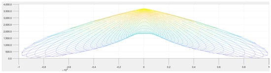
Figure 3.
MESH representation (from MATLAB) for the luminous intensity curves of the luminaire in Figure 1. The units of the orthogonal axes come from the light intensity values in polar coordinates, in cd. The axes and colors are only for suggesting the spatial distribution, and no light intensity values can be read.
The MESH object is fully rotatable, enabling examination from arbitrary viewing angles. Figure 4 shows the same distribution from a different perspective, revealing the complete envelope of flux distribution. Figure 5 presents the view perpendicular to the C0–C180 plane, completing the comprehensive spatial characterization.
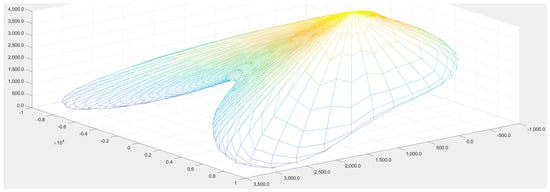
Figure 4.
MESH representation (from MATLAB) for the luminous intensity curves of the luminaire in Figure 1 from a different perspective. The units of the orthogonal axes come from the light intensity values in polar coordinates, in cd. The axes and colors are only for suggesting the spatial distribution, and no light intensity values can be read.
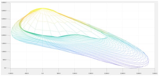
Figure 5.
MESH representation viewed perpendicularly on plane front-rear C0–C180, with red in Figure 1. The units of the orthogonal axes come from the light intensity values in polar coordinates, in cd. The axes and colors are only for suggesting the spatial distribution, and no light intensity values can be read.
Only through such complete visualization can we form an intuitive understanding of flux distribution patterns: not merely lateral (as suggested by C90–C270 dominance), but strongly diagonal, with significant implications for illumination uniformity and utilance in rectangular street geometries.
This visualization methodology applies equally to existing luminaires (analyzing actual LIDC from manufacturer data) and ideal distributions (validating computational designs). The following sections apply these tools to both cases.
Of course, the graphics in MATLAB can be rotated and studied for various angles, so that we can obtain a complete picture of the light flux distribution, an additional image being the one in Figure 4:
It can be “looked” at from all angles, including viewing C0–C180 plane, as in Figure 5:
6. Results
6.1. Case Study: PDI Analysis in Romanian Cities
Analysis of modernization projects in two Romanian cities reveals substantial variation in design quality and identifies systematic optimization opportunities. These real-world data validate that current design practices often fall short of theoretical optimum.
6.1.1. Satu Mare City Analysis
Figure 6 presents PDI values for 114 streets, ordered from lowest to highest. The distribution reveals generally competent design for most streets, with PDI clustered below 40 mW/(lx·m2). However, a significant tail extends to much higher values on the right side of the distribution.
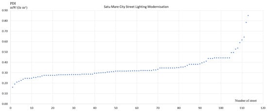
Figure 6.
PDI in mW/(lx·m2) for 114 streets in Satu Mare City.
The high-PDI outliers require case-by-case evaluation. If these represent narrow, short streets with inherently low utilance geometries, the situation may be acceptable—narrow streets inevitably require higher PDI due to geometric constraints. However, if wide boulevards appear among high-PDI cases, design revision is mandatory. Upon correction of these outliers, an average PDI around 30 mW/(lx·m2) is achievable, representing good (though not optimal) performance.
6.1.2. Iasi City Analysis
Figure 7 shows PDI distribution for 67 streets in Iasi. The pattern differs markedly from Satu Mare, suggesting different designers or luminaire families. Most PDI values exceed 40 mW/(lx·m2), with some approaching 60 mW/(lx·m2).
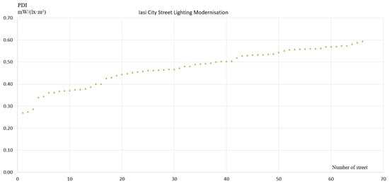
Figure 7.
PDI in mW/(lx·m2) for 67 streets in Iasi City.
Comparing the two cities, Satu Mare’s design is clearly superior, achieving systematically lower PDI values. The Iasi results demonstrate that LED technology adoption alone does not guarantee efficient design. Without explicit PDI optimization during design, even modern installations may operate far from theoretical optimum.
These case studies quantify the gap between typical current practice and achievable performance. As a detail, specific efficiency expressed in lm/W used in Satu Mare and in Iasi was almost the same, 135 lm/W.
6.2. Ideal LIDC: Computational Design and Visualization
To establish the theoretical target for LIDC optimization, we computed the ideal distribution required to achieve specified constant illumination levels: 20 lx on roadway, 10 lx on sidewalks. This reverse calculation determines luminous intensity requirements at each angular position.
6.2.1. SCATTER Visualization
Figure 8 presents the calculated ideal LIDC using MATLAB’s SCATTER function. Each point represents the magnitude of a luminous intensity vector at its angular position after transformation from spherical to Cartesian coordinates. Two lines extend from the source to representative intensity vector endpoints, providing spatial context.
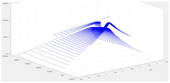
Figure 8.
An example for ideal luminous intensity vectors.
While this representation accurately depicts the data, it lacks intuitive interpretability. The three-dimensional point cloud does not immediately reveal how this distribution relates to conventional LIDC patterns familiar to lighting designers.
6.2.2. MESH Visualization of Ideal Distribution
Figure 9 applies the MESH function to the same ideal LIDC data, viewed perpendicular to the C90›C270 plane. The continuous surface representation immediately reveals familiar street lighting characteristics: strong lateral concentration with controlled longitudinal distribution.
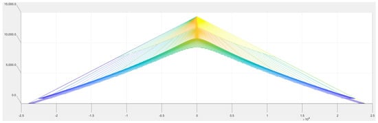
Figure 9.
MESH representation for the ideal luminous intensity vectors, viewed perpendicularly on plane C90–C270. The units of the orthogonal axes come from the light intensity values in polar coordinates, in cd. The axes and colors are only for suggesting the spatial distribution, and no light intensity values can be read.
Figure 10 shows the same MESH from a different viewing angle, optimized to reveal how the distribution addresses the specific street cross-section with sidewalks on both sides. The flux directed toward the sidewalk across the road is clearly visible, as is the distribution covering the sidewalk behind the luminaire.
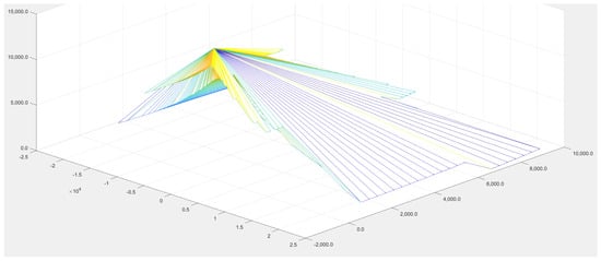
Figure 10.
MESH representation for the ideal luminous intensity vectors for a particular cross-section and pathways. The units of the orthogonal axes come from the light intensity values in polar coordinates, in cd The axes and colors are only for suggesting the spatial distribution, and no light intensity values can be read.
An important observation emerges from these visualizations: even at 1° angular resolution (both in elevation angle β and azimuth plane C), the resulting MESH surface exhibits some irregularity. This suggests that even finer angular resolution may be necessary for certain analyses, consistent with observations by previous researchers [19] regarding the dependence of calculation accuracy on angular step size.
The ideal LIDC demonstrates that perfect adaptation to a specific street geometry is theoretically possible, directing flux exactly where needed with no wasted light. This establishes the reference case for understanding real luminaire limitations and optimization potential.
6.3. Computational Validation: DIALux EVO Simulation
To validate both the ideal LIDC calculation and the minimum PDI theoretical framework, we imported the calculated distribution into DIALux EVO and simulated a representative street geometry.
6.3.1. Simulation Configuration
The test case specifies: 7 m street width, 40 m pole spacing, 12 m mounting height, −1 m overhang (luminaire positioned 1 m into the street from the curb line). The ideal LIDC from Figure 10 was converted to standard LDT format and imported into DIALux as a virtual luminaire.
6.3.2. Isolux Curve Analysis
Figure 11 presents isolux curves for the simulated installation. At first glance, the high density of contours might suggest poor uniformity. However, examining the contour values reveals that all isolux lines cluster tightly around 20 lx—exactly the target illuminance used in the LIDC calculation. This apparent non-uniformity in the graphical representation reflects the visualization scale rather than actual photometric performance.
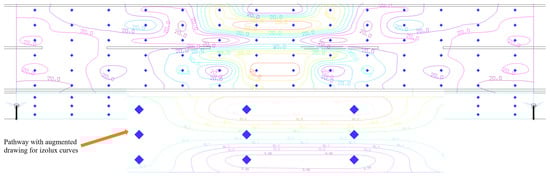
Figure 11.
The izolux curves for simulation for ideal luminaire with LIDC from Figure 10, perfectly adapted for the street and pathways considered as the study case. The color of lines are with specific meaning, different colors are used only for better visualization.
6.3.3. Quantitative Results
Figure 12 shows DIALux numerical results, which validate all theoretical predictions:
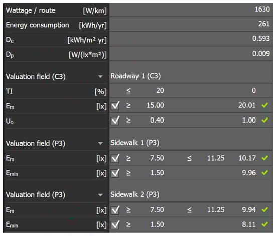
Figure 12.
Numerical results for study case simulation, with virtual perfect luminaire from Figure 10.
- Threshold Increment TI = 0, confirming that all flux is directed toward the roadway with no wasted upward light contributing to glare
- Average illuminance Em
- Overall uniformity U0
- Power Density Indicator Dp
The simulated PDI validates Equation (7) from the theoretical framework. For the specified LED efficacy (125 lm/W) and luminaire optical efficiency (90%), we predicted PDI in Section 4.2 as 8.8 mW/(lx·m2). The simulation yields PDI (named DP in DIALux) = 9 mW/(lx·m2), confirming the theoretical framework within rounding uncertainty.
Most remarkably, the simulation achieves unity uniformity—perfect constancy of illumination across the calculation surface. While no real luminaire can achieve this ideal, the simulation establishes the theoretical performance limit and quantifies the gap between actual installations and the physically achievable optimum.
7. Discussion
The results demonstrate substantial gaps between current practice, typical design, and theoretical optimum. These gaps have important implications for sustainable lighting design and the role of numerical indicators in achieving energy efficiency.
7.1. The Gap Between Practice and Potential
The case studies reveal PDI values of 30–50 mW/(lx·m2) in typical current installations. Theoretical minimum PDI for modern components (125 lm/W LEDs, 90% optical efficiency) is 8.8 mW/(lx·m2). This represents a 3–6× gap between typical and optimal performance.
Some of this gap is unavoidable. Real street geometries include features that prevent unity utilance: sidewalks requiring different illumination levels, surrounding areas needing adequate surround ratio illumination, and practical constraints on mounting heights and spacing. However, our case study comparison (Satu Mare versus Iasi) demonstrates that substantial variation exists among current designs, proving that significant optimization opportunities remain even within real-world constraints.
The literature review revealed that many published studies report even higher PDI values without recognizing them as problematic. The 66 mW/(lx·m2) measurement reported by Tomczuk et al. [14] represents 7.4× the theoretical minimum. While this may deliberately reflect narrow-beam luminaires used for specific applications, such extreme inefficiency requires explicit justification rather than being reported without comment.
Energy efficiency is not merely about LED adoption. A poorly designed LED installation operating at PDI = 50 mW/(lx·m2) wastes 5–6× more energy than theoretically necessary, negating much of LED’s technological efficiency advantage. Sustainable lighting requires both efficient sources and optimized optical design.
7.2. The Critical Role of LIDC in PDI Optimization
The ideal LIDC calculation and visualization (Figure 9 and Figure 10) demonstrate that luminous intensity distribution is not merely a photometric detail but the primary determinant of system efficiency. For given LED efficacy and optical efficiency, PDI is entirely determined by utilance, which depends solely on how well the LIDC matches the specific street geometry.
This explains several patterns observed in the literature. Gasparovsky et al. [11,13] noted PDI increasing for narrow streets and varying among installations without identifying the cause. The mechanism is now clear: narrow geometries inherently reduce utilance unless LIDC is specifically optimized for that geometry. Wide streets with multiple lanes favor high utilance, making PDI optimization easier—as evidenced by better performance in the Tayjasanant study [15], despite a lack of explicit optimization.
The three-dimensional MESH visualizations reveal why conventional two-plane LIDC representation is insufficient for utilance prediction. Diagonal flux concentration (Figure 2) can dramatically affect actual illumination patterns in rectangular street grids, yet remains invisible in C0–C180 and C90–C270 plots. Designers selecting luminaires based solely on these conventional plots cannot reliably predict system efficiency.
The resolution dependence noted in our ideal LIDC (visible irregularity at 1° steps) confirms observations by previous researchers [19] that fine angular resolution matters for accuracy. However, we can now specify why: LIDC details directly affect calculated utilance and therefore, PDI. A measurement or calculation accuracy of 20% in PDI [19] represents the difference between excellent and mediocre efficiency.
These findings suggest a revised design workflow: rather than selecting available luminaires and adjusting pole spacing/mounting height, designers should first identify the LIDC characteristics required for high utilance in the specific geometry, then select the closest available product, and finally optimize installation parameters. This LIDC-first approach reverses conventional practice but better addresses the fundamental efficiency determinant.
7.3. PDI Independence and Design Implications
The theoretical derivation (Equation (6)) confirms PDI’s independence from geometric and operational parameters that designers might assume would affect efficiency:
- PDI is independent of road class (M1–M6), contrary to assumptions in several reviewed papers [11,13].
- PDI is independent of road width per se; width affects PDI only through its influence on utilance via the LIDC-geometry matching.
- PDI is constant across dimming levels (with modern LED drivers), correcting the misconception in [12].
- PDI is intensive, not extensive; it cannot be summed across streets, contrary to the Romanian Ministry requirement that motivated this research.
This independence makes PDI particularly valuable for comparative evaluation. Unlike AECI (which correctly varies with road class and operational schedule), PDI isolates the pure efficiency of flux delivery to the target surface. Two installations can achieve identical photometric performance (meeting the same road class requirements) with different PDI values, revealing which design more efficiently delivers light where needed.
However, PDI’s independence requires correct interpretation. The frequent observation that PDI varies across installations [9,11,14] does not contradict its theoretical independence—it reveals variation in design quality and LIDC-geometry matching. PDI should be constant for a given technology level (LED efficacy, optical efficiency); deviations indicate optimization opportunity.
The implication for policy and specifications: Rather than prescribing specific luminaire types or installation geometries, standards and procurement requirements should specify maximum PDI values. This performance-based approach allows designers flexibility in achieving efficiency through LIDC optimization while ensuring genuinely efficient outcomes.
7.4. Limitations and Future Work
Several limitations constrain this work’s scope and suggest directions for extension. First, the ideal LIDC calculation assumed constant illumination targets. Real requirements specify luminance distribution rather than illuminance, and road surface reflection is non-Lambertian. Extending the optimization to luminance with realistic reflection models would address this limitation.
Second, the case studies analyzed projects that have were already designed and awaiting implementation. Prospective studies applying the LIDC-first design approach would quantify achievable improvements over conventional practice. Such studies should compare: (1) conventional approach (select luminaire, adjust installation), (2) LIDC-first approach (identify required LIDC, select closest product), and (3) theoretical optimum (ideal LIDC simulation).
Third, the ideal LIDC represents a single point in design space. Mapping the trade-off surface between utilance and other performance metrics (uniformity, glare control, surround ratio) would provide designers with quantitative guidance on acceptable compromises. Some reduction from unity utilance is necessary for practical performance; quantifying this trade-off space would be valuable.
Fourth, manufacturing constraints limit achievable LIDC characteristics. Not all theoretically optimal distributions can be realized with practical optical designs at acceptable cost. Collaboration with luminaire manufacturers to identify practically achievable distributions close to theoretical optimum would bridge the gap between academic analysis and implementable solutions.
Finally, the MESH visualization methodology could be extended beyond analysis to become a design tool. Interactive manipulation of MESH surfaces with real-time PDI calculation would provide designers with immediate feedback on how LIDC modifications affect efficiency. Such tools could accelerate optimization and improve design intuition.
8. Conclusions
This research addresses fundamental gaps in understanding and applying energy efficiency indicators for road lighting. Through theoretical analysis, advanced visualization, and computational validation, we establish both the proper interpretation of PDI and practical methods for optimization.
The Power Density Indicator is not merely a calculation requirement but an actionable design metric directly reflecting system efficiency. Its theoretical minimum, PDI, is found in Equation (7) but it must also be read from Equation (6).
The literature review revealed widespread misunderstandings: PDI treated as additive (it is intensive), varying with road class (it should not), changing with dimming (constant for modern LEDs), and analyzed without connection to LIDC (the primary determinant). These misconceptions lead to suboptimal designs that waste energy despite LED adoption. Case studies of 181 streets in Romanian cities confirm that current practice achieves 30–50 mW/(lx·m2), representing 3–6× theoretical minimum, with substantial variation demonstrating optimization opportunity.
The critical finding is PDI’s direct dependence on utilance, which is determined by LIDC-geometry matching. This mechanistic understanding explains observed patterns: narrow streets exhibiting high PDI (low utilance unless specifically optimized), wide multi-lane roads naturally favoring low PDI (inherently higher utilance), and substantial performance variation among installations (reflecting different LIDC-geometry matches). Three-dimensional MESH visualization reveals complete spatial LIDC characteristics invisible in conventional two-plane representation, particularly diagonal flux concentration that critically affects utilance.
Computational validation through ideal LIDC design demonstrates theoretical limits: unity utilance is achievable with perfectly adapted distribution, yielding PDI = 8.8 mW/(lx·m2) for relative modern components (125 lm/W LEDs, 90% optics) and perfect uniformity (U0 = 1, in Figure 12).
The practical implication is a revised design methodology: prioritize LIDC characteristics required for high utilance in the specific geometry, select the closest available luminaire, and then optimize installation parameters. This LIDC-first approach reverses conventional practice but addresses the fundamental efficiency determinant. Specifications should prescribe maximum PDI rather than specific luminaire types, enabling performance-based optimization.
Sustainable lighting requires both efficient sources and optimized optical design. LED adoption without PDI optimization wastes 3–6× more energy than necessary, negating much technological advantage. Proper application of standardized indicators, comprehensive LIDC visualization, and systematic utilance optimization can close this gap, achieving genuine, rather than superficial, energy efficiency in road lighting systems.
Author Contributions
Conceptualization, C.D.G. and I.F.; methodology, C.D.G. and I.F.; software, C.D.G.; validation, C.D.G. and I.F.; formal analysis, C.D.G. and I.F.; investigation, C.D.G.; resources, C.D.G.; data curation, C.D.G.; writing—original draft preparation, C.D.G. and I.F.; writing—review and editing, C.D.G. and I.F.; visualization, C.D.G.; supervision, C.D.G. and I.F. All authors have read and agreed to the published version of the manuscript.
Funding
This research received no external funding.
Data Availability Statement
The datasets presented in this article are not readily available because the data are part of an ongoing study with time limitations. Requests to access the datasets should be directed to C.D.G.
Conflicts of Interest
The authors declare no conflicts of interest.
Abbreviations
The following abbreviations are used in this manuscript:
| LDIC | Light Intensity Distribution Curves |
| PDI | Power Density Indicator |
| LDT | Light Distribution Data File |
| IES | Light Distribution Data File from Illuminating Engineering Society |
| AECI | Annual Energy Consumption Indicator |
References
- EN 13201-5:2015; Road Lighting—Part 5: Energy Performance Indicators. European Standard: Brussels, Belgium, 2015.
- EN 15193:2007; Energy Performance of Buildings—Energy Requirements for Lighting. European Standard: Brussels, Belgium, 2007.
- Zdunic, G. Public Lighting–Road to Energy Efficiency. In Proceedings of the 2015 5th International Youth Conference on Energy (IYCE), Pisa, Italy, 27–30 May 2015. [Google Scholar]
- Omran, M.M.; Aziz, V.; Youssef, K. Energy Efficient Lighting System. In Proceedings of the 2019 21st International Middle East Power Systems Conference (MEPCON), Cairo, Egypt, 17–19 December 2019. [Google Scholar]
- Anthopoulou, E.; Doulos, L. The effect of the continuous energy efficient upgrading of LED street lighting technology: The case study of Egnatia Odos. In Proceedings of the 2019 Second Balkan Junior Conference on Lighting (Balkan Light Junior), Plovdiv, Bulgaria, 19–21 September 2019. [Google Scholar]
- Dimitrakis, A.; Madias, E.-N.D.; Kotsenos, A.; Topalis, F.V. A New Approach to Street Lighting Design through Led Technology and Optical System Optimization. In Proceedings of the 2025 Tenth Conference on Lighting (Lighting), Sozopol, Bulgaria, 4–6 June 2025. [Google Scholar]
- Ciobanu, I.; Pentiuc, R.D. Analysis on the possibility of using retrofit solutions for increasing the energy efficiency of public lighting systems. In Proceedings of the 2016 International Conference on Applied and Theoretical Electricity (ICATE), Craiova, Romania, 6–8 October 2016. [Google Scholar]
- Panchev, H. Research and analysis of lighting and energy performance of the street lighting segment of the highway. In Proceedings of the 2021 13th Electrical Engineering Faculty Conference (BulEF), Varna, Bulgaria, 8–11 September 2021. [Google Scholar]
- Aghemo, C.; Pellegrino, A.; Fisanotti, D.; Piccablotto, G.; Taraglio, R.; Paruzzo, A.; Roscio, G. Environmental and Energy Performance of Public Lighting Installations: Results of a Measurement Campaign. In Proceedings of the 2018 IEEE International Conference on Environment and Electrical Engineering and 2018 IEEE Industrial and Commercial Power Systems Europe (EEEIC/I&CPS Europe), Palermo, Italy, 12–15 June 2018. [Google Scholar]
- Avotins, A.; Adrian, L.R.; Porins, R.; Apse-Apsitis, P.; Ribickis, L. Smart City Street Lighting System Quality and Control Issues To Increase Energy Efficiency and Safety. Balt. J. Road Bridge Eng. 2021, 16, 28–57. [Google Scholar] [CrossRef]
- Gasparovsky, D. Case-studies of the assessment of energy performance of road lighting. In Proceedings of the 2016 IEEE Lighting Conference of the Visegrad Countries (Lumen V4), Karpacz, Poland, 13–16 September 2016. [Google Scholar]
- Gasparovsky, D.; Dubnicka, R.; Janiga, P.; Barcik, M. Energy performance numerical indicators of public lighting. In Proceedings of the 2014 15th International Scientific Conference on Electric Power Engineering (EPE), Brno-Bystrc, Czech Republic, 12–14 May 2014. [Google Scholar]
- Gasparovsky, D.; Janiga, P.; Raditschova, J. Typical Values of Energy Performance Indicators in Road Lighting. Adv. Electr. Electron. Eng. 2021, 19, 134. [Google Scholar] [CrossRef]
- Tomczuk, P.; Wytrykowska, A.; Chrzanowicz, M. Analysis of Luminance Contrast Values at Illuminated Pedestrian Crossings in Urban Conditions. Energies 2023, 16, 8031. [Google Scholar] [CrossRef]
- Tayjasanant, T.; Unhavaithaya, Y.; Unhavaithaya, P.; Chamchoy, C.; Pattanapakdee, K.; Amaralikit, T.; Tepboon, P. LED Luminaires Selection for Thailand Typical Roadway Construction and Road Lighting Hierarchy. In Proceedings of the 2023 IEEE Sustainable Smart Lighting World Conference & Expo (LS18), Mumbai, India, 8–10 June 2023. [Google Scholar]
- Sujatha, V.; Sridevi, V.; Sumitha, S.; Vidhya, N.; Amirtha, M.; Dakshinamoorthi, D. Illuminating the Future: A Smart Street Light Controlling and Monitoring System Using Internet of Things Enabled Smart Sensors. In Proceedings of the International Conference on Science Technology Engineering and Mathematics, Chennai, India, 16–19 November 2024. [Google Scholar]
- Bayer, R.; Brejcha, M.; Pelánová, Z.; Zálešák, J. Road lighting design by means of genetic algorithm. In Proceedings of the 2015 16th International Scientific Conference on Electric Power Engineering (EPE), Kouty nad Desnou, Czech Republic, 20–22 May 2015. [Google Scholar]
- Wannapasert, P.; Ananwattanaporn, S.; Ngaopitakkul, A. Evaluation of Light-Emitting Diode Luminaire For Two-Lanes Roadway Lighting System. In Proceedings of the 2024 11th International Conference on Power and Energy Systems Engineering (CPESE), Nara, Japan, 6–8 September 2024. [Google Scholar]
- Zseller, V.; Samu, K. Metaheuristic of Arbitrary Luminous Intensity Distribution for Roadway Lighting Luminaires. Int. J. Simul. Model. 2023, 22, 369–380. [Google Scholar] [CrossRef]
Disclaimer/Publisher’s Note: The statements, opinions and data contained in all publications are solely those of the individual author(s) and contributor(s) and not of MDPI and/or the editor(s). MDPI and/or the editor(s) disclaim responsibility for any injury to people or property resulting from any ideas, methods, instructions or products referred to in the content. |
© 2025 by the authors. Licensee MDPI, Basel, Switzerland. This article is an open access article distributed under the terms and conditions of the Creative Commons Attribution (CC BY) license (https://creativecommons.org/licenses/by/4.0/).