Digitalization, Energy and GHG Emissions: A Path Analysis of the Impact

Abstract

The transition to a carbon-neutral society represents one of the most pressing global challenges of the 21st century, requiring a radical transformation in how energy is produced, consumed, and managed. Digitalization has emerged as a pivotal driver in energy transition, offering innovative Pathways to enhance energy efficiency and penetrate renewable energy that should lead to reduced GHG emissions. The aim of the research was to develop a model for the evaluation of digitalization impact on GHG emissions where energy serves as a mediating factor. The data of 27 European Union Member States was employed for the investigation covering the period 2014–2023. Principal Component Analysis was utilized to calculate the composite indicators of digitalization and energy. A comprehensive and systematic analysis of the complex interactions of digitalization, energy and GHG emissions was performed using a path analysis. The findings emphasized the critical role of the rebound effect of digitalization as the advantages associated with energy efficiency and the integration of renewable energy, facilitated by digitalization, are overweighted by increased energy consumption. The research ultimately contributes to a deeper understanding of how digitalization can be measured, guided, and optimized to support sustainable energy and mitigation of climate change.

1. Introduction

To address the urgent issue of climate change, the European Union has established objectives aimed at creating a climate-neutral society by the year 2050. The ambitious goal of net-zero carbon emissions aligns with the Paris Agreement on climate change and the United Nations’ Sustainable Development Goals (SDGs). SDG 13—Climate action seeks to actualize the commitment to the United Nations Framework Convention on Climate Change, aiming to attain climate-neutrality by the mid-21st century, thereby constraining the increase in global temperatures to below 2 °C, with an aspirational target of 1.5 °C [1]. Furthermore, it seeks to improve the resilience and adaptive capabilities of nations in response to climate-induced natural hazards and the ensuing calamities.

Digitalization has presently emerged as a powerful tool with the potential to significantly contribute to tackling climate change. Digital technologies such as artificial intelligence, Internet of Things (IoT), blockchain, and big data analytics can help to solve climate change issues in different ways: by improving energy efficiency, fostering renewable energy and optimizing energy consumption. The nexus between digitalization, energy and climate mitigation is in line with several SDGs, including SDG 7 “Affordable and Clean Energy”, SDG 9 “Industry, innovation and infrastructure” and SDG 13 “Climate Action”.

Many authors emphasize the advantages of innovative digital technologies, as they enable more complex and flexible energy management [2,3], while simultaneously reducing energy consumption, improving data integration, operational efficiency, and automation across various sectors. Smart energy systems utilize digital technologies to facilitate real-time monitoring of energy usage [4]. Digitalization offers insights that boost operational effectiveness and support the transition towards alternative energy sources, which are critical for reducing the carbon footprint [5]. Digital technologies facilitate innovations in production processes, intelligent design, and logistics, which optimize energy usage and strengthen the efficiency of supply chain [6]. By increasing the proportion of renewable energy in the energy market, digital technologies contribute to optimizing the energy structure, which further reduces carbon emissions [7]. In this way, digitalization contributes to climate change mitigation.

Nevertheless, the other authors emphasize substantially increased energy consumption due to the needs of data centers, artificial intelligence computations, and communication infrastructures. The rebound effects are notable, as while digital technologies can improve efficiency in some areas, they also require substantial energy and carbon-intensive materials, leading to increased overall emissions [8,9]. The reduced costs due to energy efficiency gains may encourage increased energy demand and pollution of environment [10]. Increased digitalization can also lead to higher consumption of carbon-intensive products if not managed properly [11]. Thus, energy functions as the intermediary variable connecting digitalization with climate outcomes, influencing the extent to which technological innovations can be converted into either sustainable practices or increased emissions [12]. A comprehensive understanding of these interconnections is essential for formulating policies that effectively steer the digital transition towards achieving global decarbonization objectives. This impacts a call for new measurement approaches for European Union.

However, recent studies are more oriented to various countries such as China [13,14,15], India [16], South Korea [17], Romania [18], Germany [19], and Italy [20], and use different levels of analysis: region, city, sector, company. Other researchers investigate ASEAN countries [21,22] or countries globally [3,23]. The European Union as a whole region was investigated by [6,24,25,26].

Ref. [25] evaluates the socioeconomic and resource-efficient implications of digital transformation within the public sector across the European region. Refs. [24,26] conduct an empirical analysis of the interrelationship between digital transformation and, specifically, energy security. Ref. [6] examines the investigations of digitalization on energy efficiency within the European Union. The authors in [6] limit the measurement of digitalization by Digital Economy and Society Index (DESI) and its subindexes, and they measure energy efficiency using only the indicator of energy productivity. It is notable that previous studies are lacking the complete sets of digitalization and energy indicators or are related to specific spheres of energy and with no investigation of how digitalization can impact GHG emissions through energy.

Our study addresses this gap in an original way by providing a model for the measurement of the impact of digitalization on GHG emissions in the European Union, where energy serves as a mediating factor. The paper also identifies a complex set of indicators for digitalization and an energy measurement system.

To develop a robust and empirically grounded framework, Principal Component Analysis (PCA) is employed as a research method for identifying underlying dimensions and grouping interrelated variables of digitalization and energy. PCA is used to reduce the number of initial indicators and to calculate the composite ones. Finally, Path Analysis is performed to find direct and indirect effects between digitalization, energy and GHG emissions in EU.

Research results can be beneficial for policymakers, energy managers, and stakeholders to monitor and assess the effectiveness of digitalization. The research ultimately contributes to a deeper understanding of how digital transformation can be measured, guided, and optimized to support sustainable energy and net-zero future.

This paper is combined of five sections, with the following structure: Section 1 is an introduction; Section 2 provides a review of the state-of-the-art research on the topic and is dedicated to the development of research hypotheses; Section 3 describes the data and methodology employed; Section 4 provides and discusses the main results of PCA and Path Analysis; Section 5 concludes the key findings of the study and addresses the limitations as well as outlines the potential areas for further investigation.

2. Theoretical Background and Hypotheses Development

2.1. Literature Review

Measuring the impacts of digitalization on energy efficiency and GHG emissions is a complex task, and, currently, there is no standardized approach to doing it. A recent literature analysis revealed that the authors use different levels of analysis, such as firm [17,18], industry [8,15,20], province or region [7,11,14], and country [13,21,22] when investigating issues related to the topic. Also, their investigations are related to different countries and regions of interest that lead the country-specific or region-specific data, and different models of investigation are also selected.

Recent studies were directed at countries such as China [13,14,15], India [16], South Korea [17], Romania [18], Germany [19], and Italy [20], or whole regions like ASEAN countries [21,22] and the European Union [6,24,25,26], or investigated countries globally [3,23]. For instance, ref. [15] utilized Structural Path Analysis and a Two-Way Fixed Effects Model to scrutinize the impact of industrial chain digitization on energy intensity within the manufacturing sector. Ref. [17] explored the efficiency of South Korean energy enterprises implementing digital technology, employing Stochastic Frontier Analysis and Regression Analysis for this endeavor. At the country level, ref. [23] applied Structural Equation Modeling to investigate the impact of robotics usage on environmental outcomes, utilizing data from 74 countries and regions, while [13] assessed environmental sustainability in China through the application of Dynamic Ordinary Least Squares, Fully Modified Ordinary Least Squares, and Canonical Cointegration Regression methods and [6] employed the Generalized Method of Moments system to investigate the European Twin Transition across EU Member States.

The conclusions drawn by various authors have revealed important interrelations among digitalization, energy, and GHG emissions, which are elaborated upon in detail and subsequently utilized for the formulation of hypotheses in the forthcoming subsections of this article.

2.2. Digitalization Impact on Energy Consumption, Efficiency and Renewables

Digital technologies, such as artificial intelligence, Internet of Things (IoT), blockchain, and big data analytics, have emerged as a pivotal driver in energy transition, offering innovative pathways to enhance energy efficiency and penetrate renewable energy that should lead to reduced GHG emissions.

Digitalization improves energy efficiency via automation, continuous monitoring, and systematic optimization. Ref. [3] contend that digital industrial systems contribute to a reduction in energy intensity. The implementation of smart grids and Internet of Things (IoT) augments flexibility and reliability by facilitating real-time equilibrium between supply and demand [2,27,28]. Furthermore, data analysis augmented by artificial intelligence enables the early detection of faults and the scheduling of maintenance, thereby reducing waste and minimizing downtime [29,30].

Moreover, digitalization propels the integration of renewable energy sources. Ref. [31] assert that blockchain-enabled systems foster transparent peer-to-peer energy trading, while [32] posit that digital platforms engender competitive markets for renewable energy. Ref. [2] illustrate that digital forecasting techniques and smart grid coordination mitigate intermittency and stabilize the contributions of renewable energy sources. In a similar way, ref. [33] underscore that digital innovation stimulates investment in sustainable technologies, thereby nurturing a synergistic interplay between digital advancement and energy efficiency.

Despite these advancements, digitalization markedly amplifies electricity demand. Ref. [34] indicate that information and communication technology (ICT) infrastructure constitutes a rapidly escalating share of energy consumption. Ref. [35] emphasize that the processes associated with the implementation of energy digitalization are characterized by substantial embodied emissions. Ref. [9] highlight the complex and potentially varying impacts of digital technologies on energy efficiency in manufacturing, as while some technologies can lead to reduced energy intensity, others may increase energy demand, underscoring the importance of a refined understanding of how different digital technologies impact energy consumption.

This study aims to evaluate the direct implications (whether beneficial or adverse) of digitalization on energy, leading to the formulation of the subsequent hypothesis:

H1: 

Digitalization has direct effects (positive or negative) on energy consumption, energy efficiency and energy structure.

2.3. Energy Consumption, Efficiency and Renewable Energy Impact on GHG Emissions

The enhancement of energy efficiency and the implementation of renewable energy sources remain pivotal in the mitigation of GHG emissions. Ref. [2] demonstrate that advancements in technology and digitalization contribute to improved system efficacy, thereby attenuating emissions intensity. The incorporation of renewable energy sources further reduces air pollutants and carbon emissions [30,36]. Additionally, structural transformation serves to bolster sustainability. Ref. [12] underscore that the utilization of digital technologies within smart cities and industrial sectors enhances climate resilience. Corresponding investigations by [28] indicate that the implementation of efficient energy systems promotes economic development with diminished carbon reliance.

Nevertheless, other researchers highlight the negative impact of energy consumption as energy systems continue to be significant contributors to greenhouse gas emissions. Ref. [35] assert that fossil fuels persist as the predominant source of global energy supply. It is notable that even renewable energy systems entail lifecycle emissions, particularly during their production and maintenance phases. Also, due to improved energy efficiency the decreased costs of energy services, and these services’ demands tend to increase, which can offset the efficiency gains [37]. Thus, the rebound effect can further undermine the enduring benefits associated with enhancements in efficiency [8,11]. These discussions culminate in the subsequent hypothesis:

H2: 

Energy consumption, energy efficiency and energy structure have direct effects (positive or negative) on climate change.

2.4. Digitalization Impact on GHG Emissions Through Energy

Digitalization plays a pivotal role in promoting the dissemination of renewable energy resources and fostering energy democratization [31,32]. The adoption of digital technologies supports ongoing reductions at the cost of renewable energy generation. By increasing the share of renewable energy in the energy market, digital technologies contribute to optimizing the energy structure. This shift gradually displaces fossil fuel power generation, thereby lowering the energy demand on both the supply and demand sides.

Conversely, digitalization possesses the potential to indirectly intensify greenhouse gas emissions when it is integrated with fossil fuel-dependent systems. Ref. [35] highlight that the energy consumption associated with information and communication technologies significantly increases overall carbon dioxide emissions within economies reliant on fossil fuels. The rebound effects are notable, as while digital technologies can improve efficiency in some areas, they also require substantial energy and carbon-intensive materials, leading to increased overall emissions [8]. Firms adopt more efficient technologies, and the reduced costs may encourage greater usage; ultimately, this leads to increased energy demand and pollution of the environment [10]. In conclusion, it can be asserted that digitalization is anticipated to exert an indirect impact on GHG emissions through modifications in energy efficiency, consumption and energy structure, which culminates in the subsequent hypothesis:

H3: 

Digitalization has indirect effects (positive or negative) on GHG emissions as energy is a mediating factor.

The final theoretical research model, including all the components of impact, as well as the hypotheses developed, is presented in Figure 1:

3. Materials and Methods

3.1. Variable Selection and Data Sources

For monitoring the situation in the European Union and finding the most important linkages between digitalization, energy and GHG emissions indicators, the data of 27 EU Member States were collected from the Eurostat database for the period 2014–2023. The data period was selected in accordance with the data availability for most countries and indicators under the investigation. Indicators from Eurostat tables of sustainable development indicators (Goal 7—Affordable and clean energy; Goal 9—Industry, innovation and infrastructure; Goal 13—Climate action) as well as Environment and Energy; Science, Technology, Digital Society tables were collected for the investigation. The selection of indicators was based on the literature review and is described more in detail in the next three subsections. The absolute values of indicators were divided by GDP or capita. Following [38], our study uses country-level data as the data at the individual level in the studied countries is not publicly available in a comparable form. However, the key indicators for 2021 and 2022 were missing for all the countries; thus, this data period was not included in analysis. The descriptive statistics of the indicators, as well as their coding used in the research, are presented in Appendix A.

3.1.1. Dependent Variable

Domestic net greenhouse gas emissions (GHG emissions) that measure total national emissions of greenhouse gases, including carbon dioxide (CO₂), methane (CH₄), nitrous oxide (N₂O), and the so-called F-gases from all sectors of the GHG emission inventories [39] are used in this study, as this indicator is a European Union policy indicator, included in the EU Sustainable Development Goals for monitoring progress towards SDG 13 on climate action. This study follows [23] and uses GHG emissions measured as tons per capita, considering the complex impacts of digitalization and energy on climate change.

3.1.2. Independent Variables

Measurement of digitalization is a very complex task. Following the previous studies, the digitalization indicators used in this research include connectivity [37,40,41]-, human capital [42,43,44]-, and digital business activity [6,24,26]-related indicators. We expand our investigation to also include technological development indicators [15,17,45] for a more complex view of digital economy level in a country. The final list of 18 indicators related to different areas of digitalization is presented in

Table 1. Digitalization variables.

Digitalization Area	Variable	Measurement
Connectivity:
	Level of internet access by households	Percentage of households
	Mobile broadband internet traffic	Within the country; gigabytes per capita
Human capital:
	Employed ICT specialists	Percentage of total employment
	Female ICT specialists	Percentage of employed ICT specialists
	Employed persons with ICT education	Persons per capita
	Employed ICT specialists with tertiary education	Levels 5–8; persons per capita
	Students enrolled in tertiary education	Persons per capita
	Total number of people receiving education	Pre-primary to tertiary education, persons per capita
Digital business:
	Business enterprise R&D expenditure in high-tech sectors/GDP	All NACE activities, percentage of GDP
	Enterprises with a website	10 persons employed or more, percentage of enterprises
	Social media	10 persons employed or more, percentage of enterprises
	Cloud/cloud computing utilization	10 persons employed or more, percentage of enterprises
	Enterprises with e-commerce trading activities	10 persons employed or more, percentage of enterprises
	E-Commerce turnover	10 persons employed or more, percentage of turnover
	E-Commerce web sales: This indicates the sales made specifically through websites.	10 persons employed or more, percentage of enterprises
Technological development:
	Number of patent applications	Patent applications to the EPO, per million inhabitants
	Ratio of R&D expenditure in GDP	All sectors, percentage of GDP
	Persons employed in science and technology	Employed HRST, from 25 to 64 years, persons per capita

. These are the theoretically proposed grouping areas of digitalization variables, and they will be finally regrouped in factor analysis.

3.1.3. Mediating Variables

Energy consumption, efficiency and energy structure are the key groups of energy indicators that serve as mediators between digitalization and GHG emissions.

Energy efficiency and consumption indicators. Energy productivity, calculated as the ratio of GDP to total energy consumption, is chosen as an energy efficiency indicator as it is included in EU Sustainable Development Goals indicators [6] and is used to monitor progress towards SDG 7 on affordable and clean energy and SDG 12 on ensuring sustainable consumption and production patterns [46]. This indicator is widely used in the recent literature [6,13,25]. The other indicators in this group are related to energy consumption [26,47,48] and energy intensity [13,49,50], which is measured as the amount of energy consumed per unit of GDP, and it is the opposite indicator to energy productivity as it measures the energy inefficiency of the economy.

Energy structure indicators. Share of renewable energy consumption is the most common indicator for energy structure that represents the proportion of energy used from renewable energy sources [21,26,48]. Energy structure indicators also include natural gas consumption [37,51,52], as well as indicators of fossil fuels [45] in energy structure. The full list of energy indicators is provided in

Table 2. Energy variables.

Energy Indicators Area	Variable	Measurement
Energy consumption and efficiency:
	Energy productivity	The ratio of GDP to total energy consumption, Euro per kilogram of oil equivalent (KGOE)
	Energy consumption per capita	Primary consumption, ton of oil equivalent (TOE) per capita
	Electricity production/GDP	Gross production, kilogram of oil equivalent/EUR
	Electricity consumption/GDP	Final electricity consumption, kWh/EUR
	Residential electricity consumption/GDP	Final consumption, households, kWh/EUR
	Industrial electricity consumption/GDP	Final consumption, industry sector, kWh/EUR
Energy structure:
	Share of renewable energy consumption	Share of energy from renewable sources, percentage
	Final natural gas consumption/GDP	Megajoule/EUR
	Final oil and petroleum consumption/GDP	Kilogram/EUR
	Final solid fossil fuels consumption/GDP	Kilogram/EUR
	Share of fossil fuels in gross available energy	Percentage
	Share of solid fossil fuels in final energy consumption	Percentage

.

3.2. Research Methods

3.2.1. Principal Component Analysis

Principal Component Analysis (PCA) is a technique aimed at diminishing the dimensionality of data; to achieve this objective, it systematically transforms correlated variables into a new, smaller set called principal components [53]. According to [54], recent research has validated the superiority of the PCA-based weighting technique for the computation of composite indicators, due to its data-centric nature and its capacity to mitigate the arbitrary and subjective weighting assigned to various indicators. For example, ref. [38] employed PCA in their research to identify the latent dimensions of internet utilization, thus facilitating a reduction in the dimensionality of the dataset and categorizing variables into pertinent factors. Furthermore, PCA facilitates the development of composite indices that encapsulate the aggregate level, which can subsequently be employed to draw comparisons among various nations and regions, thereby enabling policymakers to discern optimal practices and identify areas that need to be improved [53].

PCA was used in our study to group digitalization and energy indicators and reduce dimensionality, as well as to avoid further multicollinearity of indicators. It helped to reduce the number of initial indicators and to calculate the composite ones that are required for Path Analysis when having a limited number of observations.

3.2.2. Path Analysis

Path Analysis is a model that is based on multiple linear regression equations. It disaggregates the correlation observed between independent and dependent variables into both direct and indirect effects, thereby elucidating the intricate interrelationships among the independent variables, intermediate variables, and dependent variables [55]. Thus, it is an effective technique for modeling causal relationships among multiple variables concurrently, as well as encompassing mediators [56]. As our investigation aims to measure the direct and indirect effects between digitalization, energy and GHG emissions, Path Analysis is a powerful tool for this purpose. Moreover, a comprehensively realized Path diagram serves as a framework that can be employed to guide subsequent analysis, rather than an algebraic model in statistics [57].

Path Analysis was chosen for our investigation because it provides a coherent and theoretically grounded framework for examining both direct and indirect relationships among the key constructs. This makes it well-suited to our aim of uncovering the mechanisms linking digitalization, energy use, and GHG emissions. In addition, refs. [58,59] emphasize that Path Analysis is appropriate and robust for mediation research even when sample sizes are relatively small, provided that the model remains parsimonious and theoretically justified.

In our investigation, Path Analysis is based on the system of equations that will be developed after the calculation of composite indicators in PCA. These equations will be used to measure: (1) direct effects of digitalization on energy; (2) direct effects of energy on climate change; (3) indirect effects of digitalization on GHG emissions. The results of this analysis will lead to the acceptance or rejection of our theoretical hypotheses.

4. Results and Discussion

4.1. PCA

Principal Component Analysis (PCA) was performed to calculate composite indicators of digitalization and energy to avoid multicollinearity and to reduce the number of parameters that will be used in Path Analysis. Before conducting PCA, several diagnostic procedures were performed to ensure that the data met the key statistical assumptions for multivariate analysis. First, the univariate normality of all variables was assessed using the Shapiro–Wilk test. Because PCA is based on the covariance (or correlation) structure, substantial departures from normality can bias the estimation of principal components. The Shapiro–Wilk statistic was calculated for each variable to test the null hypothesis of normal distribution. Variables with p-values below 0.05 were considered to deviate from normality. Although PCA has generally robust-to-moderate non-normality, this step provided an important diagnostic for identifying variables that did not meet the normality assumption and were therefore logarithmically transformed to achieve normality. Logarithmic transformation was applied to the following variables: Energy productivity (log_E13), Gross electricity production/GDP (log_E3), Residential electricity consumption/GDP (log_E5), Industrial electricity consumption/GDP (log_E6), Share of renewable energy consumption (log_E7), Employed ICT specialists (log_D4), Total number of people receiving education (log_D10), Business enterprise R&D expenditure in high-tech sectors/GDP (log_D11), and Number of patent applications (log_D19).

After addressing issues of univariate non-normality, the dataset was further examined for multivariate outliers, which can disproportionately affect covariance estimates and, consequently, the orientation of principal components. For this purpose, the Minimum Covariance Determinant (MCD) method [60] was employed. In this study, the detection was performed using the leverage diagnostics option, which identifies influential cases based on robust leverage values. According to the results, Ireland was identified as a multivariate outlier for PCA, so it was removed from the dataset.

In PCA, each principal component (factor) is expressed as a linear combination of the observed variables weighted by their respective coefficients. The general form of the $i$-th component is

$${\mathrm{Factor}}_i={\alpha }_{1i}{X}_1+{\alpha }_{2i}{X}_2+{\alpha }_{3i}{X}_3+\dots +{\alpha }_{pi}{X}_p$$

(1)

where ${\mathrm{Factor}}_i$ is the i-th principal component (factor score), $X_j$ represents the original observed variable j, ${\alpha }_{ji}$ denotes the coefficient (loading weight) of the variable $X_j$ for component i, and p is the total number of variables.

To select variables suitable for the Principal Component Analysis (PCA), we examined the overall Kaiser’s Measure of Sampling Adequacy (MSA). This measure indicates whether the analyzed data are appropriate for applying factor analysis. If the value of this measure is below 0.6, the correlations between variable pairs cannot be explained by other variables, and factor analysis is therefore not applicable. In our final models, the overall MSA value exceeded 0.7 for all the years under study, which confirms that the available data are suitable for conducting factor analysis.

In addition, we examined the individual MSA for each variable, which indicates whether a variable should be included in the factor analysis. If the value of this measure is below 0.5, the variable is recommended to be excluded. Therefore, only those variables with an MSA value greater than 0.5 were included in the analysis. Based on these criteria, separate PCAs were conducted for the energy and digitalization parts.

To determine how many factors could be retained, the eigenvalues of the correlation matrix were evaluated. According to the Kaiser criterion, only the factors with eigenvalues greater than 1 were retained for further analysis. For both the energy and digitalization parts, two factors were extracted, indicating that the data structure could be effectively represented by two latent dimensions in each case. Furthermore, we examined the proportion of total variance explained by the extracted factors and the Final Communality Estimates, which indicate the proportion of each variable’s variance explained by the retained factors (i.e., the common variance). The obtained results demonstrated that the extracted factors accounted for a substantial share of the total variance (all cases more than 0.5), confirming the adequacy and interpretability of the factor solutions.

PCA was conducted using the maximum likelihood (ML) extraction method, which allows estimation of the underlying factor structure that best reproduces the observed covariance matrix. This method was chosen because it provides statistical measures of model fit and enables the evaluation of factor loadings’ significance, offering greater inferential flexibility compared to others. To enhance the interpretability of the extracted components, orthogonal Varimax rotation was applied. The Varimax procedure maximizes the variance of squared loadings within each component, thereby achieving a simpler and more interpretable factor structure where each variable tends to load highly on one factor and minimally on others.

The rotated factor loadings represent the correlations between the observed variables and the extracted components, showing how strongly each variable contributes to a particular factor. Loadings close to ±1 indicate a strong association, while loadings near 0 suggest little or no relationship. For interpretation purposes, rotated loadings in our case were used. Typically, loadings with absolute values above 0.70 are considered very strong, 0.50–0.69 as moderate, and 0.30–0.49 as weak but meaningful contributions [61]. Each factor was interpreted and named based on the variables with the highest loadings, assuming that such variables share a common conceptual dimension.

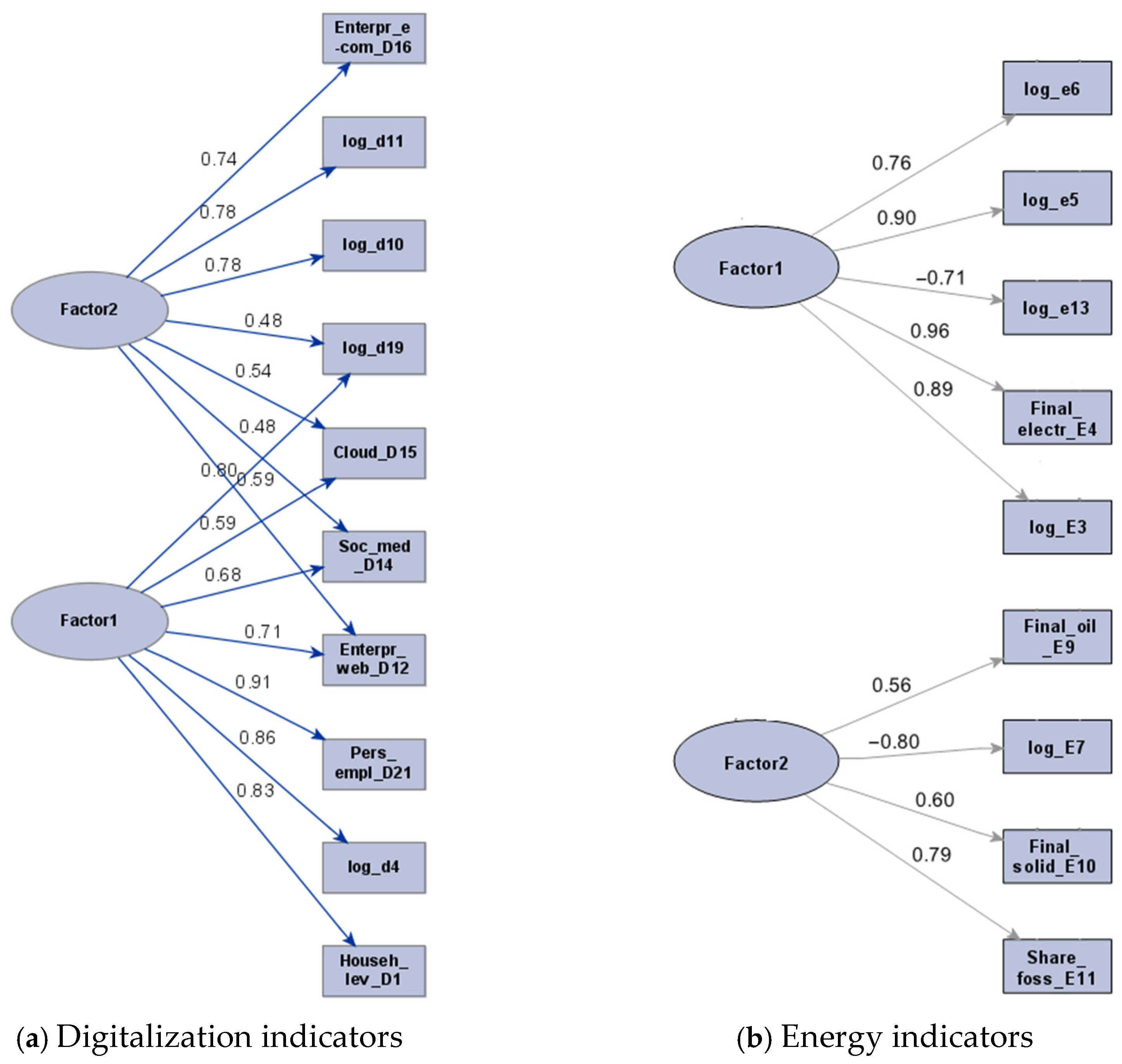
The graphical results of PCA for digitalization (a) and energy (b) indicators for 2023 are presented in Figure 2.

4.1.1. Digitalization Indicators

A Varimax-rotated PCA was applied to identify the structure of digitalization indicators. Given the scope of this paper, a detailed discussion is provided only for the PCA results of the year 2023. The analysis revealed two distinct factors that together represent the main dimensions of digitalization:

Factor 1:

$$\begin{array}{cc}\hfill pca1\_D=0.831& ·\mathrm{Househ}\_\mathrm{lev}\_\mathrm{D}1+0.855·\log \_\mathrm{d}4+0.213·\log \_\mathrm{d}10+0.219\hfill \\ & ·\log \_\mathrm{d}11+0.708·\mathrm{Enterpr}\_\mathrm{web}\_\mathrm{D}12+0.677·\mathrm{Soc}\_\mathrm{med}\_\mathrm{D}14\hfill \\ & +0.585·\mathrm{Cloud}\_\mathrm{D}15+0.227·\mathrm{Enterpr}\_\mathrm{e}\_\mathrm{com}\_\mathrm{D}16+0.798\hfill \\ & ·\log \_\mathrm{d}19+0.905·\mathrm{Pers}\_\mathrm{empl}\_\mathrm{D}21\hfill \end{array}$$

(2)

Factor 2:

$$\begin{array}{cc}\hfill pca2\_D=0.137& ·\mathrm{Househ}\_\mathrm{lev}\_\mathrm{D}1+0.276·\log \_\mathrm{d}4+0.775·\log \_\mathrm{d}10+0.777\hfill \\ & ·\log \_\mathrm{d}11+0.591·\mathrm{Enterpr}\_\mathrm{web}\_\mathrm{D}12+0.479·\mathrm{Soc}\_\mathrm{med}\_\mathrm{D}14\hfill \\ & +0.542·\mathrm{Cloud}\_\mathrm{D}15+0.739·\mathrm{Enterpr}\_\mathrm{e}\_\mathrm{com}\_\mathrm{D}16+0.483\hfill \\ & ·\log \_\mathrm{d}19+0.202·\mathrm{Pers}\_\mathrm{empl}\_\mathrm{D}21\hfill \end{array}$$

(3)

The quality criteria of the final PCA model indicate its adequacy and reliability. These criteria are presented in the tables below, including the overall and individual MSA values (

Table 3. Overall and individual MSA values for digitalization.

Kaiser’s Measure of Sampling Adequacy: Overall MSA = 0.77977976
Househ_lev_D1	log_d4	log_d10	log_d11	Enterpr_web_D12	Soc_med_D14
0.86480415	0.82775107	0.79170842	0.67959937	0.80805834	0.69488831
Cloud_D15	Enterpr_e_com_D16	log_d19	Pers_empl_D21
0.83039955	0.70540887	0.73400206	0.86562785

), the number of extracted factors (

Table 4. Number of extracted factors for digitalization.

Eigenvalues of the Correlation Matrix: Total = 10 Average = 1
	Eigenvalue	Difference	Proportion	Cumulative
1	6.22807314	5.13899338	0.6228	0.6228
2	1.08907976	0.26870895	0.1089	0.7317
3	0.82037081	0.33137278	0.0820	0.8138

) and the final communality estimates (

Table 5. Final communality estimates for digitalization.

Final Communality Estimates: Total = 7.317153
Househ_lev_D1	log_d4	log_d10	log_d11	Enterpr_web_D12	Soc_med_D14
0.70913474	0.80745649	0.64633221	0.65229051	0.85120497	0.68800117
Cloud_D15	Enterpr_e_com_D16	log_d19	Pers_empl_D21
0.63596734	0.59684666	0.86970796	0.86021084

), which show an acceptable level of variance explained. In determining the number of factors to retain, we followed the commonly applied eigenvalue-greater-than-one rule (Kaiser criterion), complemented by a theoretical assessment of the interpretability of the extracted components. This approach ensured that the retained PCA factors were both statistically sound and meaningful for subsequent Path Analysis.

PCA confirmed two factors of digitalization indicators. The developed composite indicators (factors) of digitalization are presented in Figure 2a. In general, the goal of the PCA used in our study was to reduce the number of initial indicators that are required for Path Analysis when having a limited number of observations, as well as to calculate the PCA-based weighted composite ones and mitigate the subjective weighting techniques. It should be highlighted that some of the digitalization indicators, such as Cloud computing, Social media or Enterprises with a website are overlapped between both factors; thus, both factors have relatively high loadings on these indicators. However, the first factor has the highest loadings on indicators of (1) connectivity: Internet access level by households (0.83), (2) the human capital required for successful digital business: Employed ICT specialists (0.86), Persons employed in science and technology (0.91) and (3) the extent to which businesses use digital tools: Enterprises with a website (0.71); Social media (0.68); Cloud/Cloud computing utilization (0.59). According to the framework of EC Digital Economy and Society Index (DESI) that was used in the studies of [6,24], our first factor contains the data that are related to the three different dimensions of DESI: (1) Connectivity (Internet access level by households), (2) Human capital (Employed ICT specialists, Persons employed in science and technology) and (3) Digital technologies for business (Enterprises with a website; Social media; Cloud/Cloud computing utilization). Following this framework, we combine the name for our first factor from all the three dimensions and call it “Connectivity, human capital and digital technologies for business” (pca1_D).

The second factor is more general, related to the education (Total number of people receiving education (0.78)) and technological development level of a country (Business enterprise R&D expenditure in high-tech sectors (0.78); Enterprises with e-commerce trading activities (0.74) and Total number of patent applications (0.48)). We follow [47] who named education-related indicators Education level. For the second group of related indicators, we align with the framework of [62], who referred to patent application-related indicators as technological effect, and [15], who classified R&D expenditure-related indicators as technological progress; collectively, we refer to this assemblage of indicators as technological development level. Furthermore, Enterprises with e-commerce trading activities are also included into the technological development level group, as this measure pertains to the exchange of goods or services through digital technologies. In conclusion, we call the second factor of PCA “Education and technological development level” (pca2_D).

4.1.2. Energy Indicators

Similarly to the digitalization dimension, two factors were extracted for the energy dimension. For brevity, only the PCA results based on the 2023 data are presented and discussed in detail with retained factors.

Factor 1:

$$\begin{array}{cc}\hfill pca1\_E=(-0.711)& ·\log \_\mathrm{e}13+0.886·\log \_\mathrm{E}3+0.962·\mathrm{Final}\_\mathrm{electr}\_\mathrm{E}4+0.904\hfill \\ & ·\log \_\mathrm{e}5+0.764·\log \_\mathrm{e}6+0.329·\log \_\mathrm{E}7+0.467\hfill \\ & ·\mathrm{Final}\_\mathrm{oil}\_\mathrm{and}\_\mathrm{petr}\_\mathrm{E}9+0.287·\mathrm{Final}\_\mathrm{solid}\_\mathrm{fosil}\_\mathrm{E}10-0.466\hfill \\ & ·\mathrm{Share}\_\mathrm{foss}\_\mathrm{E}11\hfill \end{array}$$

(4)

Factor 2:

$$\begin{array}{cc}\hfill pca2\_E=(-0.434)& ·\log \_\mathrm{e}13-0.026·\log \_\mathrm{E}3+0.023·\mathrm{Final}\_\mathrm{electr}\_\mathrm{E}4-0.073\hfill \\ & ·\log \_\mathrm{e}5-0.151·\log \_\mathrm{e}6-0.795·\log \_\mathrm{E}7+0.564\hfill \\ & ·\mathrm{Final}\_\mathrm{oil}\_\mathrm{and}\_\mathrm{petr}\_\mathrm{E}9+0.599·\mathrm{Final}\_\mathrm{solid}\_\mathrm{fosil}\_\mathrm{E}10+0.789\hfill \\ & ·\mathrm{Share}\_\mathrm{foss}\_\mathrm{E}11\hfill \end{array}$$

(5)

The final PCA model for the energy indicators was found to be adequate and reliable, as shown in the tables below presenting the overall and individual MSA values (

Table 6. Overall and individual MSA values for energy.

Kaiser’s Measure of Sampling Adequacy: Overall MSA = 0.69642425
log_e13	log_E3	Final_electr_E4	log_e5	log_e6	log_E7
0.79544382	0.73010168	0.78920231	0.65975973	0.69471193	0.62587033
Final_oil_and_petr_E9	Final_solid_fosil_E10	Share_foss_E11
0.65999052	0.45660366	0.65889012

), the number of extracted factors (

Table 7. Number of extracted factors for energy.

Eigenvalues of the Correlation Matrix: Total = 9 Average = 1
	Eigenvalue	Difference	Proportion	Cumulative
1	4.24542264	2.09855330	0.4717	0.4717
2	2.14686933	1.25192797	0.2385	0.7103
3	0.89494137	0.32622903	0.0994	0.8097

) and final communality estimates (

Table 8. Final communality estimates for energy.

Final Communality Estimates: Total = 6.392292
log_e13	log_E3	Final_electr_E4	log_e5	log_e6	log_E7
0.69428607	0.78586411	0.92535757	0.82315864	0.60676204	0.74064292
Final_oil_and_petr_E9	Final_solid_fosil_E10	Share_foss_E11
0.53633991	0.44086745	0.83901325

). According to the Kaiser criterion (eigenvalues > 1), two components were retained for further analysis. The variable Final_solid_fosil_E10 was retained in the model even though its individual MSA value was at the threshold, as the overall quality and adequacy of the PCA model remained higher when this variable was included.

PCA confirmed two groups (factors) of energy indicators that clearly separated (Figure 2b). The first group represents energy intensity (pca1_E), and the second group is dedicated to energy structure (pca2_E). The negative values of the indicators mean that the factor is inversely proportional to the variable. The energy intensity group contains an indicator of energy productivity (with the loading of −0.71)—the ratio of GDP to total energy consumption, as well as electricity production and electricity consumption intensity indicators. energy productivity is inverse to all other indicators of Energy intensity factor, as the more energy is consumed, the lower the value this indicator has. In that way, the energy intensity factor is inverse to energy efficiency. This factor has the highest loadings on Final electricity consumption/GDP (0.96), Residential electricity consumption/GDP (0.90), and Gross electricity production/GDP (0.90).

The factor of energy structure includes the Share of renewable energy as well as fossil fuel-related indicators. In the same way—Share of renewable energy here is inverse to all other indicators of the energy structure factor, as it measures the proportion of energy from renewable sources in total energy, while other indicators of this group measure proportions of fossil fuel-related energy. Thus, the factor of energy structure is dedicated to measuring the fossil fuel-based energy structure, which is opposite to renewable energy. This factor has the highest loadings on Share of renewable energy consumption (−0.80) and Share of fossil fuels in gross available energy (0.79).

As the analysis revealed that there are only two factors of energy indicators, the individual indicator Primary energy consumption per capita (E2), which was not suitable for factor analysis, is used to represent the energy consumption in this study. Primary energy consumption per capita [24,26,47] measures energy needs and covers the energy consumption by end users such as industry, transport, and households [63]; thus, it is a suitable representative for energy consumption of a country.

4.2. Path Analysis

The linear equations for the Path Analysis were developed in accordance with the theoretical hypotheses, forming the conceptual basis for the structural model. After the theoretical framework had been defined, the structure of the equations was specified to ensure consistency between the theoretical model and statistical identifiability. In Path Analysis, the structure of equations is determined by the number of estimated parameters to ensure that the model remains identified. The final model represents a case of an over-identified model, where the number of estimated parameters is smaller than the number of moments. The number of moments is calculated as k(k + 1)/2, where k is the number of observed variables. The difference between the number of moments and the number of estimated parameters represents the model’s degrees of freedom (df). In this study, the Path model was constructed so that df > 0, ensuring that the model is over-identified and that its fit can be statistically evaluated. In such a case, it is possible to assess not only the parameter estimates themselves but also the overall quality of the model by comparing the estimated covariance matrix with the empirical covariance matrix. Although including additional variables would be theoretically desirable, doing so would have reduced the model’s degrees of freedom to zero, resulting in a just-identified model where fit cannot be statistically assessed. Therefore, the current, more parsimonious model was retained to preserve over-identification, enable empirical evaluation of model fit, and ensure stable estimation given the small sample size.

After evaluating all quality and suitability criteria, only the equations demonstrating the most meaningful and theoretically justified relationships were included in the Path model. Given the structure of the available data and the small sample size, the number of regressors had to be deliberately kept limited to ensure that the Path model would remain identifiable and retain positive degrees of freedom. We used the adjusted coefficient of determination (Appendix B) as a diagnostic tool to verify that each equation contributed sufficient explanatory power, since equations with very low R² values would undermine model fit. For these reasons, only relations with the highest adjusted R² values and clear theoretical relevance were selected for inclusion in the model.

In certain cases, variables with statistically non-significant p-values were retained in the regression equations, as their inclusion was theoretically substantiated and consistent with the conceptual framework of the study. This approach is also justified by the small sample size, where p-values may lack sufficient power to detect existing effects. Ref. [64] highlights that in mediation models, the primary focus should be placed on the magnitudes of the direct and indirect effects rather than on p-values, further supporting the suitability of this approach for the aims of our study.

Regression analysis (Appendix B) has shown that GHG emissions (

Table A2. Regression of GHG emissions with independent energy variables.

Dependent Variable: GHG_Climate_change = Primary_Energy_E2 pca2_E pca1_E
Root MSE					1.42865
R-Square					0.5264
Dependent Mean					6.43043
Adj R-Sq					0.4517
Coeff Var					22.21706
Parameter Estimates
Variable	DF	Parameter Estimate	Standard Error	t Value	Pr > |t|
Intercept	1	−0.29872	1.55644	−0.19	0.8498
Primary_Energy_E2	1	2.60104	0.59632	4.36	0.0003
pca2_E	1	0.62154	0.39656	1.57	0.1335
pca1_E	1	−0.41912	0.38315	−1.09	0.2877

) can be predicted using the data of energy intensity and energy structure composite indicators, as well as the individual indicator of energy consumption (Adj. R-Sq = 0.4517). However, GHG emissions regression with predictors of digitalization (

Table A3. Regression of GHG emissions with independent digitalization variables.

Dependent Variable: GHG_Climate_change = pca1_D pca2_D
Root MSE					1.77658
R-Square					0.2291
Dependent Mean					6.43043
Adj R-Sq					0.1521
Coeff Var					27.62772
Parameter Estimates
Variable	DF	Parameter Estimate	Standard Error	t Value	Pr > |t|
Intercept	1	6.62442	0.38438	17.23	<0.0001
pca1_D	1	0.80848	0.50091	1.61	0.1222
pca2_D	1	0.65858	0.50485	1.3	0.2069

) had a very low value of Adj. R-Sq (0.1521); thus, the direct effects of Digitalization on GHG emissions were not included in the final model. Regression analysis also revealed that energy intensity (Adj. R-Sq = 0.5132) (

Table A4. Regression of energy intensity.

Dependent Variable: pca1_E = pca2_D pca1_D
Root MSE					0.60182
R-Square					0.5575
Dependent Mean					−0.01686
Adj R-Sq					0.5132
Coeff Var					−3569.80214
Parameter Estimates
Variable	DF	Parameter Estimate	Standard Error	t Value	Pr > |t|
Intercept	1	−0.16707	0.13021	−1.28	0.2141
pca2_D	1	−0.34575	0.17102	−2.02	0.0568
pca1_D	1	−0.6529	0.16968	−3.85	0.0010

) and energy consumption (Adj. R-Sq = 0.2683) (

Table A5. Regression of energy consumption.

Dependent Variable: Primary_Energy_E2 = pca2_D pca1_D
Root MSE					0.44399
R-Square					0.3348
Dependent Mean					2.54565
Adj R-Sq					0.2683
Coeff Var					17.44117
Parameter Estimates
Variable	DF	Parameter Estimate	Standard Error	t Value	Pr > |t|
Intercept	1	2.59687	0.09606	27.03	<0.0001
pca2_D	1	0.27899	0.12617	2.21	0.0388
pca1_D	1	0.19627	0.12518	1.57	0.1326

) can be predicted using the composite indicators of Connectivity, human capital and digital technologies for business as well as Education and technological development level, while these were not suitable predictors for the energy structure (Adj. R-Sq = 0.0510) (

Table A6. Regression of energy structure.

Dependent Variable: pca2_E = pca2_D pca1_D
Root MSE					0.81783
R-Square					0.1372
Dependent Mean					0.16208
Adj R-Sq					0.051
Coeff Var					504.59292
Parameter Estimates
Variable	DF	Parameter Estimate	Standard Error	t Value	Pr > |t|
Intercept	1	0.11658	0.17694	0.66	0.5175
pca2_D	1	−0.31993	0.2324	−1.38	0.1838
pca1_D	1	−0.16256	0.23059	−0.7	0.4890

).

In parallel, by adjusting the regression equations of the Path Analysis model according to the theoretical hypotheses and the requirements of model identifiability, a corresponding regression analysis model equation was constructed and tested to verify whether it met all regression model assumptions. This procedure was carried out to ensure the reliability of the regression equations and to prevent poor model quality in the Path Analysis. For this purpose, potential outliers were examined, and cases of Sweden, Finland, and Luxembourg were identified as strong outliers and, therefore, were excluded from the analysis to ensure the robustness and reliability of the estimated Path coefficients. All these countries had extremely high technological development levels according to their indicators, while Sweden and Finland were also extremely good in terms of renewable energy. During the estimation of the Path Analysis models, these countries proved to be highly influential observations that exerted an unusually strong impact on the estimated coefficients. Influence diagnostics (e.g., leverage and residual patterns) showed that their presence substantially distorted the regression relationships. As is well-established, Path Analysis and OLS-based regression models become unreliable when dominated by such influential cases, because parameter estimates become unstable and the mediation structure is compromised.

Additionally, the multicollinearity of the independent variables in the equations was examined using the variance factor (VIF), which quantifies how much the variance of a regression coefficient is increased due to collinearity among predictors. All calculated VIF values were below 4, indicating an acceptable level of multicollinearity. In addition, the absence of autocorrelation in the regression residuals was tested using the Durbin–Watson (D) statistic. The obtained D value was approximately 2, and the corresponding p-value was not statistically significant, indicating that neither positive nor negative autocorrelation was present in the residuals. In addition, the heteroscedasticity of the regression model residuals was examined using the test of first- and second-moment specification, which indicated adequate model properties and confirmed that the assumption of homoscedasticity was satisfied. Moreover, the normality of residuals (Shapiro–Wilk test) and the equality of their means to zero (t-test) were tested, confirming that the residuals met the assumptions of normal distribution and zero-mean. The corresponding hypotheses regarding the normality and zero-mean value of residuals were verified and not rejected, indicating that the model satisfies the classical linear regression assumptions. The results of the regression analysis and the assessment of its assumptions for 2023 are provided in Appendix C, supporting the adequacy of the model specification.

This led to the following structural linear equations with standardized coefficients of the final Path Analysis model (

Table 9. Path Analysis model.

No.	Model Equation
1	GHG_Climate_change = b1 × Primary_Energy_E2 + b2 × pca2_E + b3 × pca1_E + e1
2	pca1_E = b5 × pca1_D + b6 × pca2_D + e2
3	Primary_Energy_E2 = b4 × pca1_D + b7 × pca2_D + e3

).

The codes of composite and single indicators used in the Path Analysis model are given in

Table 10. Path Analysis model indicators.

Code	Name	Single/Composite
GHG_Climate_change	GHG emissions	Single
pca1_D	Connectivity, human capital and digital technologies for business	Composite
Pca2_D	Education and technological development level	Composite
E2	Energy consumption	Single
Pca1_E	Energy intensity	Composite
Pca2_E	Energy structure (fossil fuel-based)	Composite

.

The coefficients b₁ to b₇ in Table 9 represent the direct standardized effects among variables in the Path Analysis model, where each b quantifies the direct influence of one variable on another while controlling for all other relationships in the model. The standardized effects generally range in magnitude from −1 to +1, representing the full possible span of relationships from strongly negative to strongly positive.

According to the conventions proposed by [65], standardized effect sizes of around 0.10 are considered small, those of around 0.30 are moderate, and those of 0.50 or greater are large in practical significance. Negative (inverse) coefficients indicate that as one variable increases, the other tends to decrease, suggesting an opposing or reversing relationship between them. The closer a negative value is to −1, the stronger the inverse association. In contrast, positive coefficients imply that increases in one variable are associated with increases in another, with values near +1 representing a powerful direct connection. Occasionally, standardized coefficients greater than 1 can appear when variables share very high correlations or when measurement error inflates relationships. Such coefficients do not indicate a computational mistake, but they should be interpreted cautiously as indicators of exceptionally strong relationships.

In this investigation, we focus exclusively on standardized effects, as they allow for the direct comparison of the relative strength and direction of relationships across variables measured on different scales. Standardization removes the influence of measurement units, making it possible to evaluate which Path exert the strongest impact within the overall model. Because all coefficients are expressed on the same standardized scale, the direct, indirect, and total effects can be meaningfully compared to assessing the relative contribution of each pathway to the dependent variable. This comparability enables a clearer understanding of how much of the total influence is transmitted through mediating variables versus direct causal links.

The formulas used to calculate the indirect standardized effects are presented in

Table 11. Calculation of indirect standardized effects.

Effect Type	Path	Formula
Indirect Effect pca1_D → GHG_Climate_change	pca1_D → Primary_Energy_E2 → GHG_Climate_change + pca1_D → pca1_E → GHG_Climate_change	(b4 × b1) + (b5 × b3)
Indirect Effect pca2_D → GHG_Climate_change	pca2_D → Primary_Energy_E2 → GHG_Climate_change + pca2_D → pca1_E → GHG_Climate_change	(b7 × b1) + (b6 × b3)

.

Furthermore, the goodness of fit of the Path Analysis model was evaluated for each year of the study (from 2014 to 2023, excluding 2021 and 2022 due to insufficient data). The models were estimated using the maximum likelihood (ML) method, with an identical structure across years, including three endogenous and six exogenous variables and a total of nineteen parameters. The key fit indices assessed were the Chi-square (χ²) statistic and its probability (p-value), the Goodness-of-Fit Index (GFI) and its adjusted version (AGFI), the Root Mean Square Residual (RMR/SRMR), the Root Mean Square Error of Approximation (RMSEA) with its 90% confidence interval, and the Comparative Fit Index (CFI), Normed Fit Index (NFI), and Non-Normed Fit Index (NNFI).

Across all years, Chi-square test p-values were greater than 0.05, indicating that the models did not significantly differ from the observed data and could therefore be considered an acceptable fit. Other indices generally supported this conclusion: most GFI values exceeded 0.90, SRMR values remained below 0.08, CFI was not less than 0.9, and RMSEA confidence interval [0; 0.05], suggesting a satisfactory overall model fit.

However, the number of observations was relatively small, which limits the reliability and generalizability of the fit indices. With such sample sizes, fit statistics can become unstable, and goodness-of-fit measures may either overestimate or underestimate the true model quality [58]. For this reason, we focused on the magnitude of effects, rather than on p-values or fit indices. All interpretations are therefore based on the estimated direct and indirect effects. Nevertheless, the overall fit indices across the analyzed years indicate that the specified Path model provides a reasonably good fit to the available data (a detailed summary of fit indices for each year is presented in Appendix D).

For each year, both the direct and indirect standardized effects were calculated to evaluate the structure and strength of relationships among the model variables over time. To assess the stability of the estimated coefficients, the bootstrap method was applied, generating 1000 resamples of similar size. For each resample, both the Path model coefficients and the corresponding effect estimates were recalculated, and their confidence intervals were estimated. 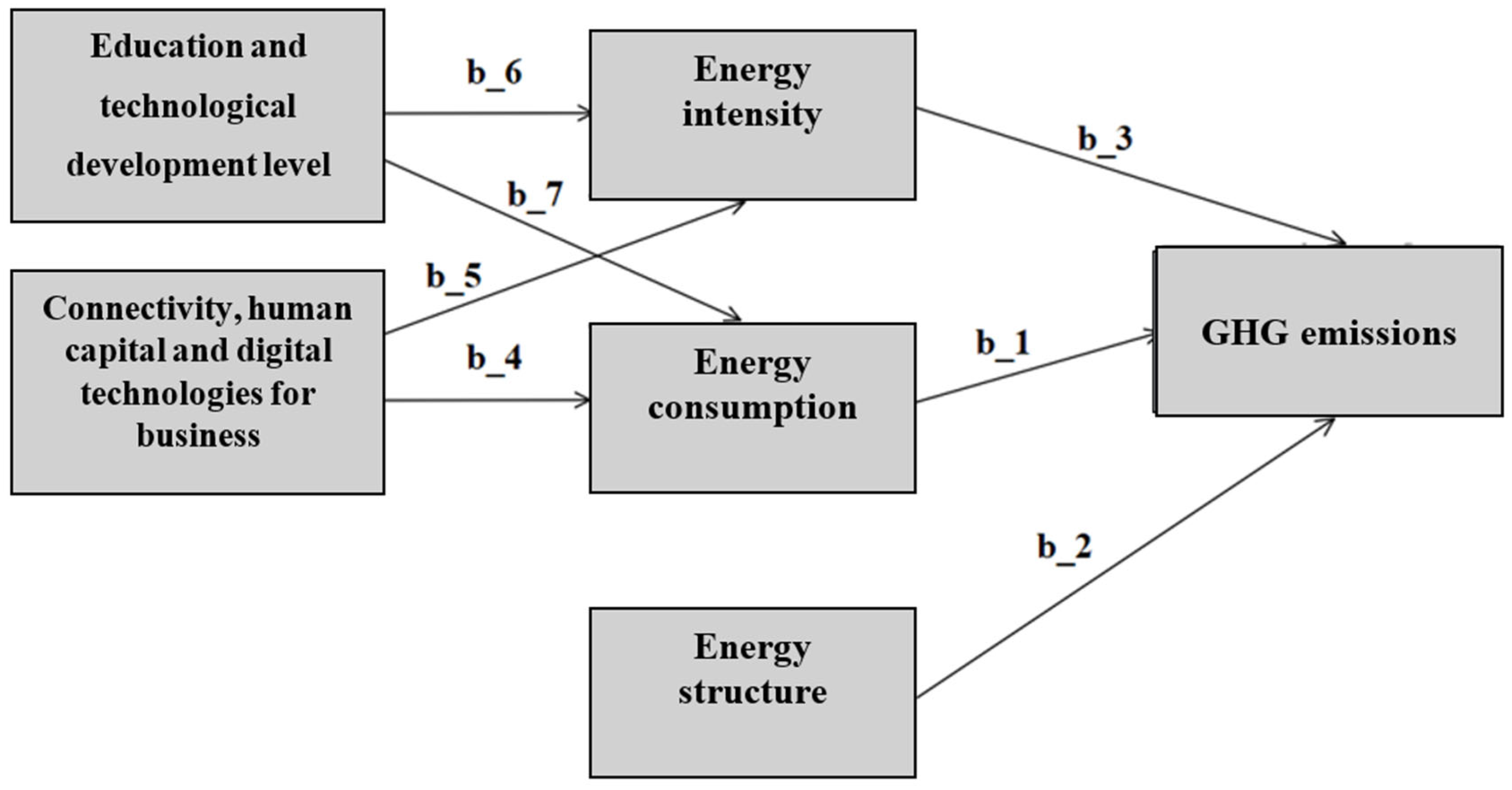The summarized results of all Path Analysis effects are presented in Appendix E, while the Path Analysis model diagram with the corresponding coefficients is shown in Figure 3.

In the following sections, we provide a more detailed discussion of the direct and indirect effects observed throughout all investigated years.

4.2.1. Direct Effects

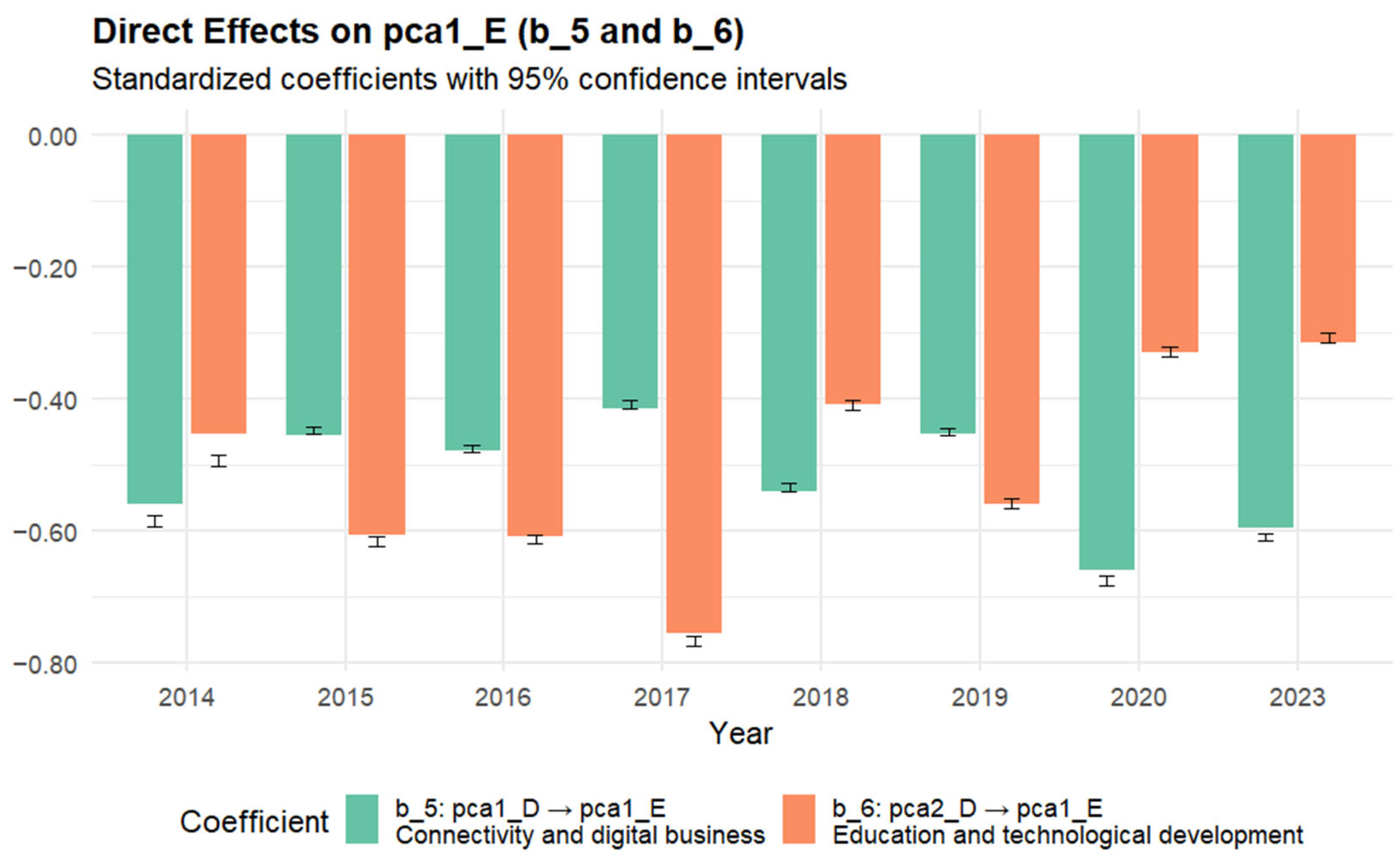
Both digitalization components, Connectivity, human capital and digital technologies for business (parameter b₅), as well as Education and technological development level (parameter b₆), had direct effects on energy intensity composite indicator (Appendix E). As parameter values are negative, this means that the higher the digitalization level is, the lower the energy intensity we have. Thus, digitalization has positive direct effects on energy efficiency. Digitalization improves energy efficiency via automation, continuous monitoring, and systematic optimization. This is in line with [3], who investigated the impact of digitalization on haze pollution and emphasized that digitalization contributes to a reduction in energy intensity. Figure 4 illustrates the estimated sample coefficients, shown as the bar height, along with the bootstrapped 95% confidence intervals of the mean coefficient estimates, with the bootstrapped mean value located at the center of the interval.

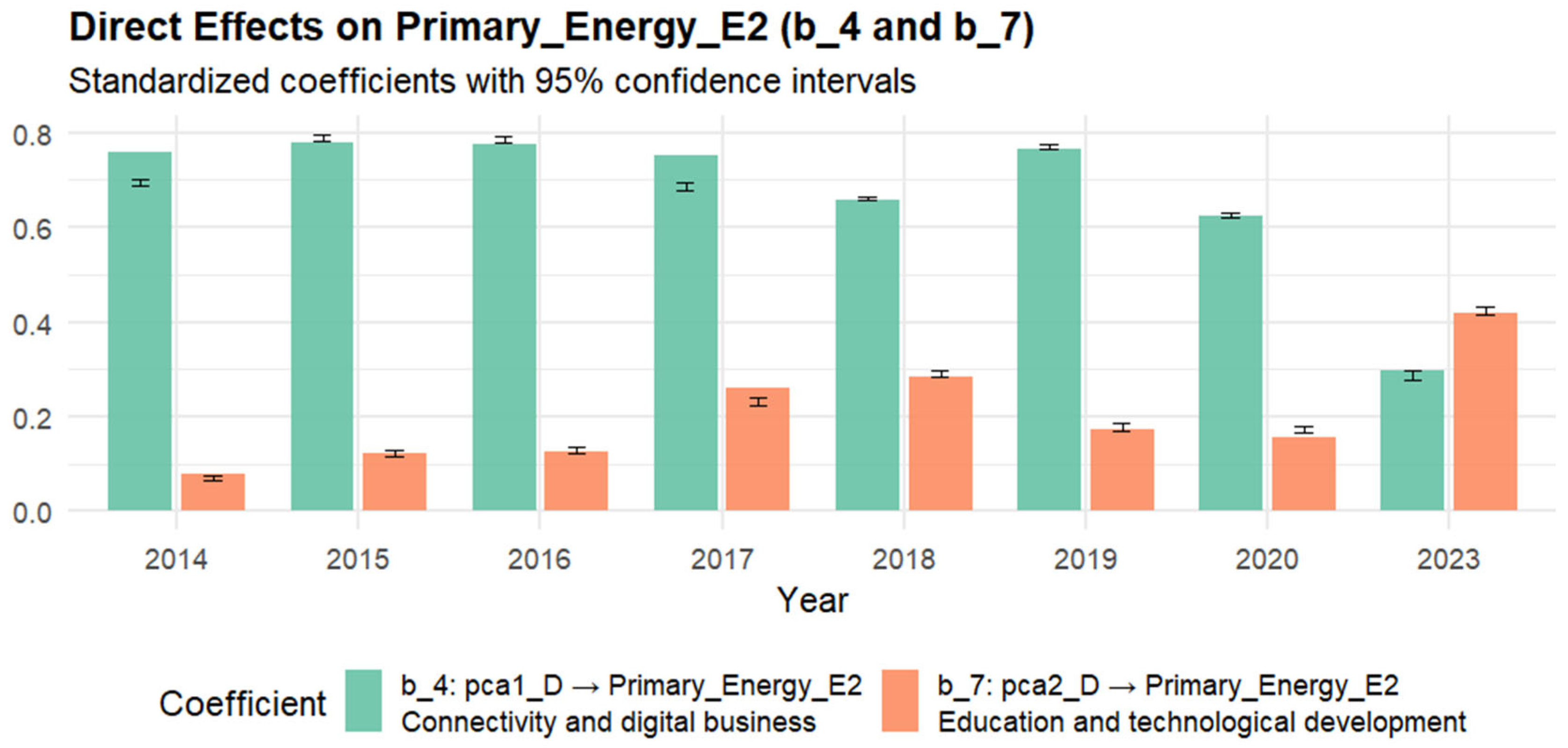
The positive direct effects of Connectivity, human capital and digital technologies for business (parameter b₄) were determined on energy consumption in 2014–2023, while the Education and technological development level (parameter b₇) was not significant for the years 2014–2020, but it became significant and even higher than Connectivity, human capital and digital technologies for business in 2023 (Appendix E). This shift could reflect a transition from digital expansion in data centers, devices, and networks that require energy to smart transformation when education and sustainable technology matter more. Nevertheless, both digitalization factors had positive direct effects on energy consumption in 2023 (the higher the level of digitalization is, the more energy is consumed).

This can be explained by the two main effects: First, it is in line with [35], who emphasized that the implementation of energy digitalization requires a lot of computational power and is associated with high energy consumption; and second, it can be explained by consumer behavior. Since improvements in energy efficiency led to a reduction in the marginal costs of energy services, it can be anticipated that the utilization of such services will increase, consequently offsetting some of the expected reduction in energy consumption. This phenomenon is commonly referred to as the direct rebound effect [66]. However, even if there is no direct rebound effect, there exist numerous additional factors that may contribute to the economy-wide reduction in energy consumption being less pronounced. For instance, the financial savings accrued from reduced energy consumption may be allocated towards the acquisition of alternative goods and services that similarly necessitate energy for their provision. Depending on the context in which energy efficiency improvement is realized, these so-called indirect rebound effects may manifest in various forms, including increases in the output of certain sectors, transitions towards more energy-intensive goods and services, and increases in energy consumption attributable to decreased energy prices and accelerated economic growth [66]. The comprehensive rebound effect resulting from an improvement in energy efficiency encapsulates the aggregation of these direct and indirect effects.

Figure 5 displays the estimated coefficients together with the bootstrapped 95% confidence interval for parameters b₄ and b₇.

As the regression analysis has shown that there is no linear relation between digitalization and energy structure (Appendix B), the direct effects of digitalization on energy structure were not tested in Path Analysis. On the other hand, the literature review suggested that digital technologies can be a powerful tool for fostering renewable energy as digital forecasting techniques and smart grid coordination mitigate intermittency and stabilize the contributions of renewable energy sources [2], blockchain-enabled systems foster transparent peer-to-peer energy trading [31] and digital platforms engender competitive markets for renewable energy [32]. However, the insignificant linear relationship between digitalization and energy structure may reflect nonlinear or lagged effects as renewable integration requires years of investment and the integration of renewable technologies to the existing power grids requires substantial upgrades, such as smart meters, advanced sensors, real-time data platforms, and digital control systems. These upgrades involve high costs, complex coordination among utilities, and technical challenges; thus, grid integration progresses slowly, limiting its immediate impact of digitalization on the overall energy structure. Also, it could be influenced by national energy policies, pricing systems and regulatory frameworks and require more governmental initiatives for pushing renewable energy forward. All these obstacles can weaken any direct statistical relationship between digitalization and changes in the national energy structure.

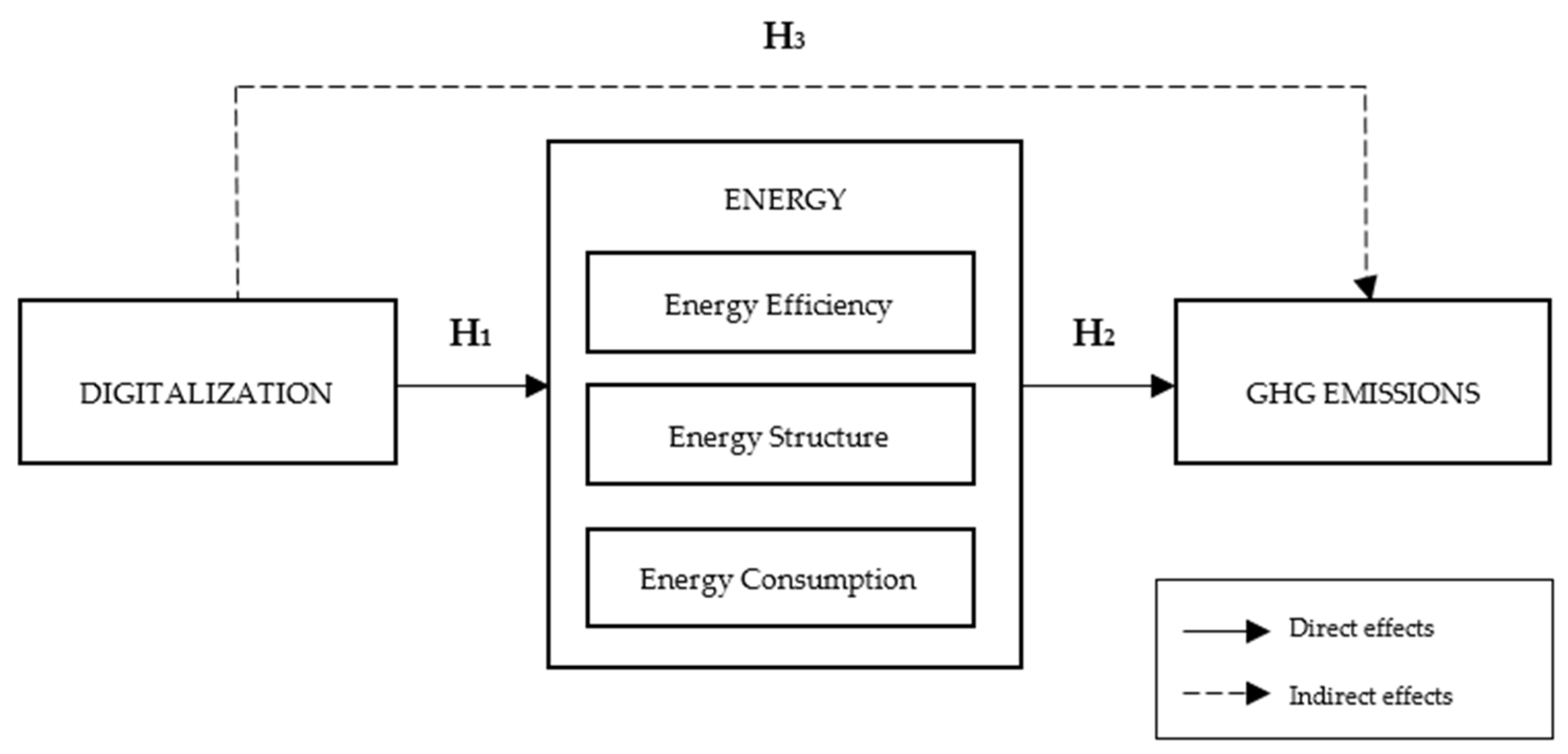
To summarize, the hypothesis “H1: Digitalization has direct effects (positive or negative) on energy consumption, energy efficiency and energy structure” was partially confirmed as digitalization had direct effects on energy intensity and energy consumption, but there was no significant impact of digitalization on energy structure.

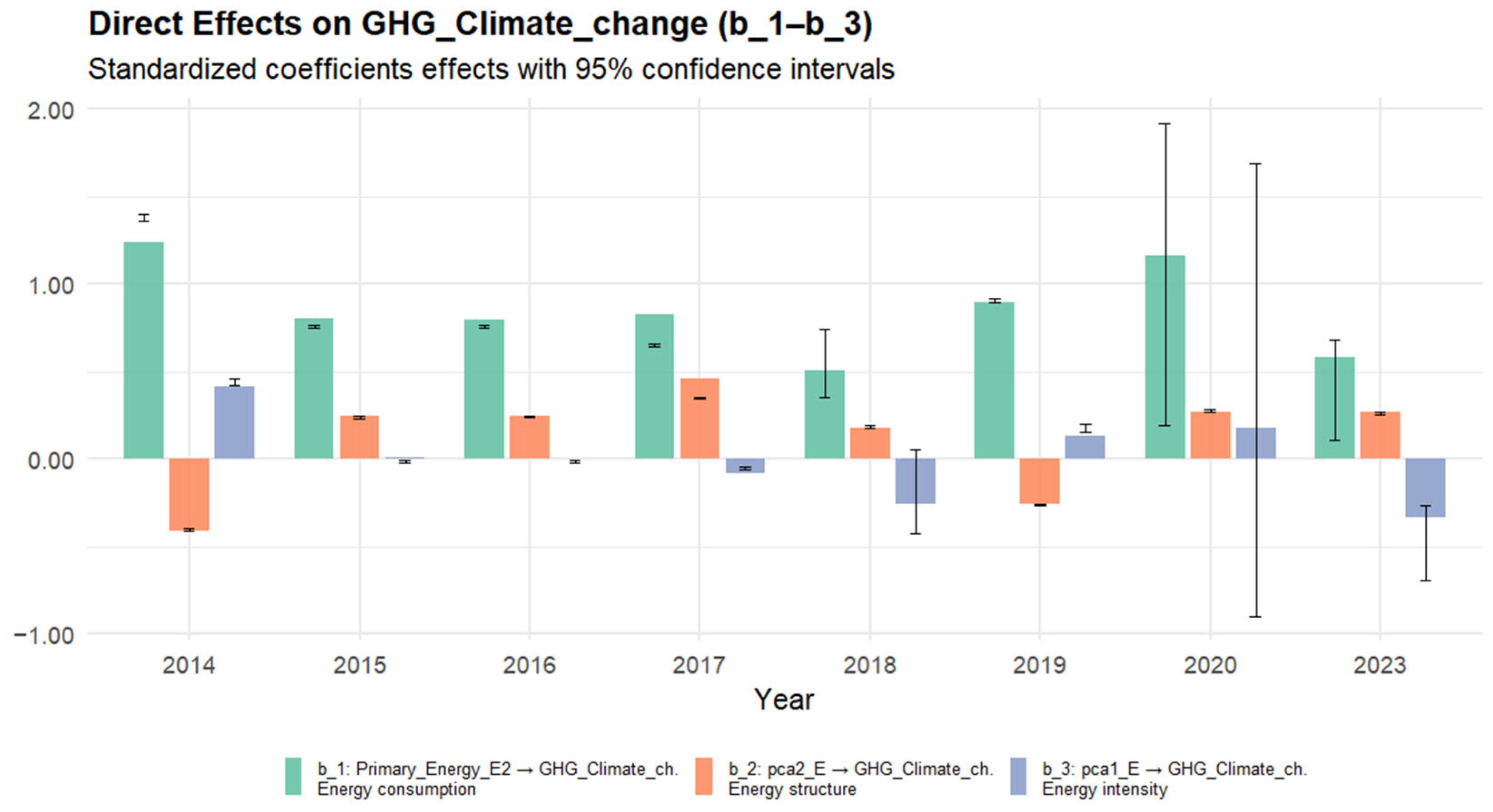
The Path Analysis has revealed that direct effects of energy intensity (parameter b₃) on GHG emissions were not significant (Appendix E). Thus, our research did not confirm the conclusions of [2], who emphasized that significant improvements in the efficiency of energy production, distribution, and consumption not only optimizes the use of resources but also enables the reduction in greenhouse gas emissions.

Despite this, the positive direct effects of energy consumption (parameter b₁) on GHG emissions were detected (Appendix E). This means that the higher the energy consumption is, the more GHGs are emitted. Thus, the effects of energy efficiency on GHG emissions are not as important as the rebound effects of energy consumption, and this is in line with [9], who highlights the complex and potentially varying impacts of digital technologies on energy efficiency in manufacturing, as while some technologies can lead to reduced energy intensity, others may increase energy demand.

Energy structure (parameter b₂) has significant effects on GHG emissions (Appendix E). During most of the period of analysis, the effects are positive, meaning that the more fossil fuel-based energy structure there is, the more GHG are emitted. Thus, a renewable energy-based energy structure helps to reduce the amount of GHG emissions and adds its value to climate change mitigation. It confirms the positive repercussions of renewable energy consumption on environmental outcomes [36]; thus, structural transformation serves to bolster sustainability. It is highlighted that in some years (2014, 2018), parameter b₂ is negative, and that generally means that even renewable energy systems entail lifecycle emissions, particularly during their production and maintenance phases.

In conclusion, the hypothesis “H2: energy consumption, energy efficiency and energy structure have direct effects (positive or negative) on GHG emissions” was partially confirmed. However, it is notable that the effects of energy consumption on GHG emissions are much higher than those of Energy structure, as b₁ > b₂ in all the year models (Figure 6); thus, the rebound effect of energy consumption undermines the benefits associated with renewable energy.

4.2.2. Indirect Effects

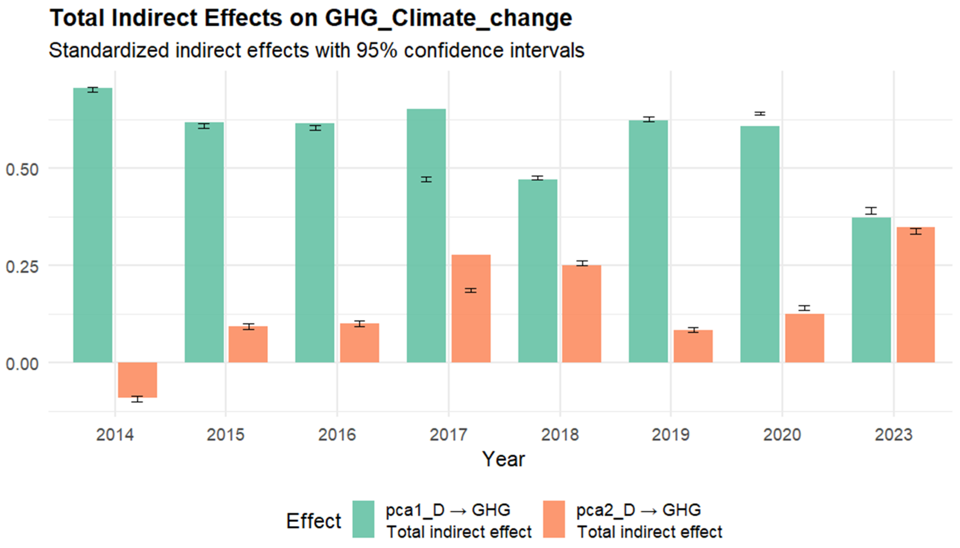
The indirect impacts of digitalization on GHG emissions were also evaluated. Connectivity, human capital and digital technologies for business had significant positive indirect effects on GHG emissions, while the effects of Education and technological development level were not significant for the period of 2014–2020 and became significant in 2023 (Appendix E). Thus, the hypothesis “H3: Digitalization has indirect effects on GHG emissions, as energy is a mediating factor” was confirmed.

The indirect effects of digitalization on GHG emissions are illustrated in Figure 7. The positive effects mean that the higher the level of digitalization is, the more GHGs are emitted. These indirect effects can be explained by the mediating effect of energy consumption: The higher the digitalization level, the more energy is consumed, and this leads to higher GHG emissions. These findings are in line with other authors [8,10], who stated that while digital technologies can improve efficiency in some areas, they also require substantial energy and carbon-intensive materials, leading to increased overall emissions [8]; also, due to improvements in digitalization, the costs are reduced, and this leads to increased energy demand and pollution of the environment [10]. Our study has shown that the rebound effect plays a crucial role here, as energy efficiency and renewable energy penetration benefits gained because of digitalization are outweighed by increased energy consumption and this results in higher GHG emissions.

5. Conclusions

GHG emissions can be influenced by digitalization, and energy efficiency plays a crucial role as a mediator in this relationship. A complex measurement framework for digitalization and energy indicators has been established, leading to the development of composite digitalization indicators encompassing Connectivity, human capital and digital technologies for business alongside Education and technological development level, while energy indicators have been categorized as energy intensity, energy structure and energy consumption.

The Path Analysis model developed for the European Union Member States has confirmed the direct and indirect effects between digitalization, energy and GHG emissions components. Both digitalization components exerted direct effects on energy intensity and energy consumption, thereby demonstrating that digitalization has the potential to contribute positively to the improvements in energy efficiency, but at the same time, it can lead to increased energy consumption that underscores the importance of the rebound effect. However, no significant impact of digitalization on energy structure was detected, indicating that more inclusion of digital strategies in the penetration of renewable energy is required, as it remains an ongoing process within the EU Member States. The direct effects of energy intensity on GHG emissions were not significant as energy efficiency was undervalued in relation to energy consumption and energy structure. The positive direct effects of energy consumption on GHG emissions have been observed, indicating that the increase in energy consumption correlates with a rise in GHG. While the energy structure has also significant effects on GHG emissions, the impacts associated with energy consumption were markedly more pronounced. The positive indirect effects of digitalization on GHG emissions were observed, highlighting that a heightened degree of digitalization correlates with increased GHG emissions. Our research has demonstrated that the rebound effect is pivotal in this dynamic, as the advantages associated with energy efficiency and the integration of renewable energy, which are facilitated by digitalization, are outweighed by the rise in energy consumption.

Policy implications. The model for the multidimensional evaluation of relations between digitalization, energy and GHG emissions was developed for monitoring the situation in the European Union as a distinct geopolitical entity. The findings of this research can be beneficial for EU policymakers, energy managers, and stakeholders to monitor and assess the effectiveness of digitalization, while guiding its trajectory to optimize its contributions to energy efficiency and structure.

The integration of digital technologies requires collaborative efforts among stakeholders. Emphasizing financial incentives and regulatory frameworks can enhance the effectiveness of energy-efficient practices. Policymakers and industry stakeholders are encouraged to design digitalization policies that consider the direct and indirect impacts of digitalization to achieve better environmental outcomes. The findings suggest that policymakers should consider connectivity, human capital and digital technologies for business, as well as high-level education and technological development progress as critical components in their energy management strategy.

There is a need for policymakers to focus on promoting the ICT sector to enhance energy efficiency. By investing in digital technologies, the government can facilitate better energy management and contribute to environmental sustainability. However, there is a tendency to focus on the positive impacts of ICTs, such as enhanced energy efficiency, while often neglecting the negative impacts, including the energy consumption of ICTs themselves. This gap in policy awareness suggests a need for a more integrated approach to understanding the full spectrum of ICT impacts on energy efficiency and environmental sustainability. Policymakers need to be cautious about the implications of increased digitalization. They should consider strategies to minimize the rebound effect to ensure that improvements in energy efficiency do not lead to greater overall energy consumption.

There is also a need to ensure the continuous development of ITC professional skills, as simply having ICT specialists does not necessarily improve energy efficiency in firms. Professional development for ITC specialists should be initiated by governments and included in lifelong-learning programs or provided by firms so that these specialists can effectively participate in the digital transformation process. Digitalization will not automatically lead to improvements in energy efficiency, as achieving these benefits requires active management and strategic integration of digital technologies into existing processes.

Digital technologies for business can significantly improve energy efficiency; however, energy consumption associated with data centers and Cloud computing can lead to increased overall energy use and highlights the need for careful implementation to ensure that the gains in operational efficiency do not lead to unintended environmental impacts. Companies need to focus on reducing their energy footprint to align better with ESG principles. To effectively leverage digital technologies for energy efficiency, it is important to integrate energy optimization measures within companies and across supply chains. This integration is crucial for enhancing decision-making and achieving corporate environmental sustainability goals.

While digital technologies are effective in directly promoting energy efficiency, their impact on GHG emissions is indirect. This indicates that the overall environmental impact still requires additional strategies. High-level education and the ability to effectively participate in technological progress is crucial here. Prioritizing research and development efforts to advance low-carbon technologies in the industrial sector is crucial. There is a need for integrated carbon management strategies that consider both sector-specific and supply-chain-wide measures. This approach can help identify carbon abatement potentials and support the low-carbon transition.

Limitations and future research directions. Nevertheless, this model faces several limitations. Firstly, it uses a relatively small dataset, as comparable information can only be collected at the country level of EU Member States. Secondly, the model does not include control variables such as economic development, industrial structure, income per capita, policy environment or economic structure, which can be important influencing factors. Thirdly, the countries having extremely high technological development levels (Sweden, Finland, Luxembourg, Ireland) were identified as strong outliers and therefore, were excluded from the model to ensure the robustness and reliability of the estimated Path coefficients. Consequently, prospective research endeavors could expand the scope of interest to incorporate additional countries globally, categorizing them according to their levels of technological development and necessarily including the control variables to avoid the omission of possible influencing factors. Expanded research, including a bigger dataset and a more complete panel structure, would allow highly digitalized countries to be included without being identified as outliers in dynamic or FE/RE models. Also, the utilization of panel-data approaches or dynamic modeling techniques would provide stronger causal identification, particularly with respect to temporal evolution, simultaneity, and endogeneity.