Short-Term Residential Load Forecasting Based on Generative Diffusion Models and Attention Mechanisms

Abstract

Accurate short-term prediction of residential power consumption is imperative for efficient energy system management. However, the complexity of high-resolution load data, nonlinear dynamics of load fluctuation, and external factor interactions pose challenges to traditional load forecasting methods. This work introduces a diffusion model-based and attention mechanism-enhanced temporal forecasting framework to address the volatility and uncertainty in load patterns. The proposed model enhances the noise robustness via diffusion processes, captures multi-scale temporal features through temporal convolutional networks, and adaptively focuses on critical time steps using attention mechanisms. Further, a dynamically weighted loss function is designed to improve both the prediction accuracy and latent representation quality. Experiments on multiple real-world residential load datasets show that the proposed model always outperforms benchmarks, reducing on average the mean absolute error (MAE) by 47.4%, symmetric mean absolute percentage error (SMAPE) by 39.7%, and mean absolute percentage error (MAPE) by 57.6%. It also achieves the superior root mean square error (RMSE) and Pearson correlation coefficient (PCC) performance, validating its effectiveness for high-resolution and multi-modal load forecasting.

1. Introduction

Accurate short-term residential load forecasting (STRLF) has become increasingly critical in modern power system optimization, particularly in the context of rapid urbanization and the pervasive integration of energy-intensive smart appliances [1]. The exponential growth of smart home devices has led to unprecedented levels of granularity and availability in residential energy consumption data. By 2024, for instance, over 1.06 billion smart meters had been deployed worldwide, enabling real-time monitoring of household electricity usage at minute-level resolution. While this surge in data availability provides rich information for more accurate forecasting, it also introduces substantial challenges. The complexity, high dimensionality, and non-stationary nature of high-resolution load data significantly increase the difficulty of modeling, particularly when capturing the intricate temporal dependencies inherent in household energy consumption patterns. Load patterns are influenced by multiple factors, including household activities, appliance usage, and weather variations [2]. Notably, residential load volatility is especially pronounced during peak hours, where fluctuations can exceed 40% within a 15 min window [3]. These characteristics highlight the pressing need for advanced STRLF approaches, as conventional forecasting methods struggle to handle such high volatility and complex nonlinearity [4]. Consequently, resilient and adaptive prediction models are required, capable of comprehensively incorporating atmospheric variables, household behavior patterns, and terminal utilization trends. This challenge also emphasizes the need to extract meaningful features from large-scale datasets while accurately modeling their dynamic interactions. Designing an efficient forecasting framework that addresses these challenges is thus imperative, not only to manage short-term residential load fluctuations but also to adapt to high-resolution data with time-series noise, information redundancy, and external variable variations.

The increasing penetration of renewable generation and distributed energy resources (DERs) has fundamentally reshaped modern grid management and scheduling paradigms. For example, solar photovoltaic systems alone contributed 4.5% of global electricity generation in 2022. However, the inherent intermittency of solar power introduces significant uncertainty into load forecasting, as outputs fluctuate with cloud cover and other environmental factors [5]. This uncertainty underscores the need for STRLF models that can rapidly adapt to fluctuations in power supply and accommodate unstable energy inputs, particularly in grids with high renewable energy penetration where balancing supply and demand is highly complex. Additionally, the emergence of demand response programs introduces further complexity. Utilities have increasingly implemented dynamic pricing schemes to incentivize consumers to shift electricity usage across different time periods, thereby optimizing grid operation [6]. Such load-shifting behaviors, driven by price variations, exhibit nonlinear characteristics, presenting additional challenges for forecasting models to accurately capture behavioral changes and predict load fluctuations. Traditional statistical approaches, including autoregressive integrated moving average (ARIMA) and support vector regression models, often fall short in these contexts due to their limited ability to capture nonlinear temporal relationships and multivariate interactions, leading to reduced performance on high-dimensional, time-varying consumption datasets. In addition, recent studies have highlighted that neural network-based methods, such as long short-term memory (LSTM) and random forest ensembles, can significantly outperform conventional statistical approaches in complicated smart grid environments, achieving higher accuracy and robustness in forecasting [7].

Deep learning techniques can offer promising solutions for the STRLF. Transformer-based architectures, which excel at capturing long-range dependencies, have shown significant potential for various time-series forecasting tasks. However, their quadratic computational complexity often imposes substantial computational and memory costs, limiting their applicability on large-scale datasets [8]. Generative diffusion models, on the other hand, have demonstrated notable robustness to noise, particularly when handling corrupted or degraded data. They can effectively reduce mean absolute error (MAE) and improve overall forecasting accuracy [9,10,11]. Despite these advantages, diffusion models alone are insufficient for temporal feature alignment and multi-scale consistency, especially when load variations are influenced by complex, multidimensional external factors. To address similar challenges, Zheng et al. have also proposed an attention-enhanced feature engineering strategy with stacked gated recurrent units (GRUs), achieving over 27% accuracy improvement for electric vehicle charging stations by mitigating big data fluctuations and capturing multi-sequence correlations [12]. In addition, Liu et al. have introduced a coupled forecasting framework based on Gaussian implicit spatio-temporal blocks with attention, demonstrating its superiority in capturing multivariate residential load dependencies and reducing prediction errors [13]. Hybrid models that combine temporal convolutional networks (TCNs) with attention mechanisms have also shown efficacy in capturing both short-term and long-term dependencies in time-series data [14]. Nevertheless, such hybrid models still struggle with multi-scale temporal alignment, particularly in scenarios like next-day load fluctuations induced by appliance usage cycles, where variations occur across multiple time scales.

Furthermore, growing attention has been directed toward the integration of electric vehicles (EVs) and renewable energy sources into forecasting frameworks. Rizi et al. have demonstrated that deep learning-based net load forecasting, considering both distributed renewable energy and EV charging strategies, could greatly enhance the power system flexibility, achieving over 50% improvement in flexibility metrics [15]. These insights emphasize the critical role of advanced forecasting models not only in improving predictive accuracy but also in supporting system-level operational objectives such as flexibility and stability.

To address the challenges of data sparsity, nonlinear dynamics, and high uncertainty in STRLF, we propose a novel framework named Diffusion-based and Attention-enhanced Temporal Modeling (DATeM). It improves forecasting accuracy through multi-feature fusion and noise suppression, while simultaneously strengthening temporal dependency modeling to ensure stability and generalization under complex load patterns. The primary contributions of this work are summarized as follows:

• A diffusion-based uncertainty modeling strategy is introduced to reconstruct reliable input features from noisy and missing data. The forward diffusion process simulates data degradation, while the reverse process iteratively restores features, enhancing model robustness and adaptability to uncertainty in load patterns.
• A TCN-based sequence encoder is developed to efficiently model high-dimensional, variable-length sequences. Leveraging TCN’s parallelism and stable gradient propagation, the encoder enhances temporal feature extraction while maintaining computational efficiency.
• An attention-augmented GRU decoder is designed to facilitate multi-scale temporal modeling. Integrating attention mechanisms assists the GRU in capturing long-sequence dependencies, thereby improving both prediction accuracy and generalization.
• Extensive experiments on real-world residential load datasets, evaluated using MAE, root mean square error (RMSE), and Pearson correlation coefficient (CORR), demonstrate that the proposed DATeM framework outperforms existing methods in terms of accuracy, robustness, and practical applicability.

In this study, we focus on short-term residential load forecasting, aiming to accurately predict the household power consumption in the near future. More specifically, the forecasting task is defined as predicting the residential load for the next 30 min based on the previous 240 min of multi-source inputs, including historical load, photovoltaic generation, battery charging/discharging power, and meteorological variables such as temperature, solar irradiance, and wind speed. These data are collected from the StoreNet dataset with a 1 min resolution, allowing us to fully capture the fine-grained temporal dynamics of household energy behavior.

The remainder is organized as follows: Section 2 reviews existing works in STRLF, Section 3 presents an overview of the proposed DATeM framework, Section 4 exhibits the theoretical basis for each module, Section 5 describes data sources, experiment setup, and results while comparing DATeM with benchmark methods, and Section 6 concludes the work, respectively.

2. Related Work

The residential load forecasting at short-term horizons has become increasingly critical for the ower system optimization. With the proliferation of smart meters and extensive integration of renewable energy sources, the complexity and stochasticity of residential load data are greatly increased, with higher demands on the robustness and adaptability of forecasting models.

Early studies typically focus on statistical learning methods through linear assumptions and probabilistic modeling. Yu et al. proposed a ridge regression framework based on the sparse coding, enhancing the next-day and next-week total load forecasting accuracy by sparsifying features [16]. However, its linear assumption struggles to capture the complicated nonlinear dynamics of user behaviors. To lower the computational complexity, Stephen et al. developed a predictor combining Markovian transitions with behavioral theories, thereby eliminating the need for environmental data and historical demands, but it was constrained by the generalization ability of classification models [17]. To achieve the temporal alignment, Teeraratkul et al. proposed a dynamic time warping method, which optimizes the energy consumption pattern alignment and reduces the number of representative groups by 50%, yet cannot well maintain the computational efficiency for high-dimensional data [18]. Due to Gaussian process (GP)’s probabilistic modeling capabilities, Xie et al. constructed an integrated GP framework, incorporating both multi-source data and adaptive communication control to improve the hourly forecasting efficiency in DER scenarios [19]. Van et al. pointed out that while the dynamic GP reduces computational burdens by updating hyperparameters via the moving window, it degrades the ability to capture peak loads [20]. Meanwhile, traditional time series methods such as ARIMA models are constantly improved. Lu et al. employed the recursive forgetting factor least squares (RFFLS) approach to simplify the parameter estimation, validating its real-time forecasting adaptability on data from the real world [21]. However, its inherent linearity remains insufficient to handle highly stochastic disturbances.

Recently, deep learning methods have significantly enhanced the capability of nonlinear time series modeling. Kong et al. were among the first to apply long short-term memory (LSTM) networks to household-level load forecasting [22], with gating mechanisms effectively capturing short-term fluctuation patterns, thereby surpassing traditional methods in accuracy on public datasets. Building upon sequence-to-sequence (Seq2Seq) learning, Xu et al. incorporated a dedicated temporal attention module to better model distant dependencies, where the encoder–decoder structure integrates periodic features, thereby leading to the improved multi-step sequence forecasting accuracy [23]. Convolutional neural networks (CNNs) have also been used in the time series domain. Cheng et al. designed a CNN-squeeze-and-excitation module that combines the micro-meteorological data with multi-channel inputs, demonstrating its multi-factor analyzing capability across eight community datasets [24]. Meanwhile, Zuo et al. validated the advantages of TCN in the community battery system load forecasting, where the dilated causal convolution structure improves the training efficiency by 90% compared to LSTM in single-step forecasting while maintaining the accuracy in multi-step forecasting by expanding the receptive field [25]. In terms of the spatial dependency modeling, Lin et al. proposed a graph neural network (GCN) framework that captures inter-household latent correlations without requiring prior geographical knowledge, outperforming baseline models in both aggregate and individual load forecasting tasks [26]. However, despite some advancements in the accuracy and efficiency, the above methods still face challenges in the uncertainty quantification and dynamic adaptation of STRLF.

To adapt to uncertainties introduced by renewable energy penetration and abrupt changes in user behaviors, there have been some interests in probabilistic modeling and real-time adaptation. Tajalli et al. proposed a multi-agent system for the cloud-fog computing collaboration, using the distributed deep learning to generate prediction intervals for stochastic sources (e.g., wind and solar energy), achieving low-latency responses through the fog computing, but relying on a complicated communication architecture [27]. Regarding the uncertainty quantification for aggregators, Dab et al. developed a model-driven method based on the probability density function generation, determining flexibility requirements through confidence intervals, with experiment results where the additive Gaussian process reduces the forecasting error by 26% compared to the Prophet model [28]. The integration of non-intrusive load monitoring (NILM) with the forecasting has also emerged. Langevin et al. designed a two-stage framework that the first stage uses a variational autoencoder (VAE) to disaggregate the total load into appliance-level data, and the second stage combines VAE with TCN to perform the forecasting [29]. In particular, on the UK-DALE dataset, the proposed approach improves the MAE and mean absolute percentage error (MAPE) by 16% and 19%, respectively, since the deep generative architecture further advances the probabilistic modeling. Khodayar et al. used LSTM to acquire non-discrete probability profiles for grid parameters, outperforming traditional point estimation methods in reliability metrics such as continuous ranked probability score within a 68-node system [30]. Despite the above advancements, existing methods still face challenges of model rigidity and high computational overhead in the dynamic environment, necessitating the lightweight and adaptive framework for real-time forecasting and uncertainty-aware optimization.

As mentioned above, while existing works have made progress in the statistical learning, artificial intelligence and uncertainty quantification, the following limitations remain:

• Traditional statistical methods rely on linear assumptions and manual feature engineering, which are intractable for modeling high-dimensional nonlinear load dynamics.
• Deep learning methods improve the forecasting accuracy but primarily focus on deterministic outputs, lacking the end-to-end probabilistic modeling capability.
• Uncertainty quantification and dynamic adaptation techniques are typically isolated, lacking the effective integration with multi-scale temporal feature extraction.

Therefore, the proposed forecasting model tries to enhance the feature robustness through the diffusion process, encode temporal patterns via multi-scale TCN, and decode dynamic dependencies with the attention-based GRU, thereby achieving the unified noise suppression, multi-scale modeling and real-time adaptation in high-resolution load forecasting and providing a reliable solution for highly volatile scenarios.

3. Framework Overview

The developed deep neural forecasting framework aims to improve both the prediction precision and operability in STRLF, comprising three core components as the data collection, model optimization, and practical application, as illustrated in Figure 1. Each component plays a crucial role in enhancing forecasting accuracy, reliability, and operational feasibility.

Figure 1. Distributed residential load forecasting framework and local training process. It illustrates the distributed architecture of residential load forecasting (left) and the local training process (right), encompassing the data collection, preprocessing, TCN-based temporal feature extraction, diffusion modeling, attention-based decoding and backpropagation optimization, respectively.

First, the data collection is conducted by deploying smart meters and temperature-humidity sensors in residential homes. Smart meters are responsible for recording the household electricity consumption at the frequency of one minute, including the real-time power consumption, historical load, and power and voltage data, thus providing rich information for capturing household load patterns. In addition, the environmental data collected by temperature-humidity sensors (e.g., indoor and outdoor temperature and humidity) can reflect the impact of weather changes on the household electricity usage, especially during seasonal transitions or extreme weather conditions, which is crucial for the subsequent model training and optimization. Data fusion is performed on the collected data, encompassing feature fusion and data normalization. Feature fusion enhances data interpretability and reduces model dimensionality, whilst data normalization ensures consistency in data distribution, thereby guaranteeing stability throughout the model training process. By integrating all these diverse data sources, the inherent relationship between the household electricity usage and environmental factors can be analyzed, providing sufficient input for the subsequent deep learning models. In particular, the household electricity data is denoted as ${\mathbf{L}}_t\in {\mathbb{R}}^d$, where d is the feature dimension and t represents the time step, while the environmental data (such as temperature and humidity) is denoted as ${\mathbf{E}}_t\in {\mathbb{R}}^m$, where m is the dimension of environmental data. The input vector ${\mathbf{X}}_t$ is concatenated as

$${\mathbf{X}}_t=\left[{\mathbf{L}}_t,{\mathbf{E}}_t\right],$$

(1)

which will be next input into the neural network for training and prediction.

Next, when the data is processed by the neural network for training and inference, we use an architecture that combines diffusion models, TCN, and attention-enhanced GRU decoders to cope with the challenges brought by high-dimensional features, nonlinear dynamics and long-term dependencies in the household load data. In the encoding phase, the proposed model uses TCN as the encoder for processing the high-dimensional and variable-length sequence data. In particular, the TCN generates hidden states ${\mathbf{z}}_0$ through convolution operations, i.e., $z_0=\mathrm{TCN}\left({\mathbf{X}}_t\right)$, which extract features from time series data through convolution operations and activation functions. Especially for handling the long sequence data, TCNs are more efficient than traditional recurrent neural networks (RNNs) or LSTMs while avoiding the gradient vanishing issue. More especially, the TCN could enhance the model’s temporal perception by using the multi-layer convolution, better capturing the temporal feature of load data.

Then, the diffusion model iteratively optimizes the forward and backward processes, enabling the reconstruction of reliable input features from noisy or incomplete data. It extracts features consistent with the characteristics of household load data and enhances the model’s robustness to noise and outliers, not only refining the input features but also improving the prediction accuracy and reliability under high uncertainties. The forward and backward processes of diffusion models are described as

$$q\left({\mathbf{z}}_t\right|{\mathbf{z}}_{t-1})=\mathcal{N}\left({\mathbf{z}}_t;{\mathbf{z}}_{t-1},{\beta }_t\mathbf{I}\right),$$

(2)

and

$$p\left({\mathbf{z}}_{t-1}\right|{\mathbf{z}}_t)=\mathcal{N}\left({\mathbf{z}}_{t-1};{\mathbf{z}}_t-{\alpha }_{t}f\left({\mathbf{z}}_t\right),{\sigma }_t\mathbf{I}\right),$$

(3)

respectively, where ${\mathbf{z}}_t$ is the intermediate representation in the diffusion process, ${\beta }_t$ is the noise variance adjustment parameter, $f\left({\mathbf{z}}_t\right)$ denotes the noise removal function learned during the training, and ${\alpha }_t$ and ${\sigma }_t$ are hyperparameters controlling the backward process, respectively. Through the above steps, the diffusion model effectively eliminates the noise from input data and recovers clean input features via the reverse process.

Finally, to further enhance the decoder’s performance, we introduce an attention-enhanced GRU decoder, which integrates attention mechanisms with GRU, automatically focuses on the most relevant temporal features, improves the feature selection capability, and thus enhances the capability of GRU in learning long-term sequential relationships. In particular, the GRU component employs reset and update gates to adaptively balance historical information and instantaneous fluctuations, allowing the decoder to capture rapid local variations commonly found in residential load profiles. By combining the denoised latent representation produced by the diffusion model with external weather-related features, the decoder can incorporate both contextual factors and short-term disturbances during the state-updating process. This design enables the decoder to extract stable temporal dependencies while remaining sensitive to abrupt changes, thereby improving forecasting robustness and precision. The final prediction result is expressed as ${\widehat{y}}_s=\mathrm{Model}\left({\mathbf{X}}_{\mathrm{input},t}\right)$. With the accurate load prediction, household users can adjust their electricity usage habits, avoid peak periods, optimize energy consumption and thus reduce electricity costs. Power companies, on the other hand, can optimize the grid resource allocation and enhance the grid stability through improved forecasting results, which is particularly crucial in the background of sustainable and renewable resources, since the load prediction is significant for optimizing the demand response and energy scheduling.

4. Diffusion-Attention Temporal Modeling

The proposed DATeM is a dwelling-level short-term load estimation framework based on the TCN, the diffusion probabilistic model (DPM) and the attention mechanism. In particular, it extracts the latent representation of the feature embedding sequence through the TCN encoder, enhances the robustness of latent representation using the diffusion process, and dynamically focuses on key information through the attention decoder to generate high-precision load prediction results. The workflow can be grouped into four stages as follows:

• Feature extraction: The latent representation of the input sequence is extracted through the TCN encoder.
• Diffusion enhancement: Noise perturbation is applied to the latent representation, and the denoising process is conducted.
• Dynamic decoding: The prediction result is generated based on the attention mechanism.
• Weight adaptation: An adaptive loss weighting mechanism is integrated to concurrently enhance both the forecasting precision and latent feature discriminability.

In particular, the pseudocode is expressed in Algorithm 1. Starting from the input sequence $\mathbf{X}\in {\mathbb{R}}^{B\times L\times d}$, the latent representation ${\mathbf{z}}_0=E\left[\mathbf{X}\right]$ is first extracted through the TCN encoder, which effectively encodes long-term contextual relationships and fine-grained local features through the integration of dilated causal convolutions and stacked residual layers. Next, the latent representation ${\mathbf{z}}_0$ is enhanced in the robustness through the diffusion process; in particular, the diffusion step t is randomly sampled, and Gaussian noise $ϵ\sim \mathcal{N}\left(\mathbf{0},\mathbf{I}\right)$ is added, generating the noisy latent representation ${\mathbf{z}}_t=\sqrt{{\overline{\alpha }}_t}{\mathbf{z}}_0+\sqrt{1-{\overline{\alpha }}_t}ϵ$. The noise ${ϵ}_{\theta }=M\left(z_t,t\right)$ is then predicted using the diffusion model M. Then, based on the denoised latent representation ${\mathbf{z}}_t$, the attention decoder dynamically focuses on crucial features extracted from the encoder’s output using a multi-head attention framework and generates the prediction result $\widehat{\mathbf{Y}}=D\left({\widehat{\mathbf{z}}}_0\right)$ by combining it with GRU. Finally, the dynamic weighted loss function is utilized to optimize both the prediction precision and quality of latent representation, where the prediction loss $L_{\mathrm{MSE}}=\parallel \mathbf{Y}-\widehat{\mathbf{Y}}{\parallel }^2$ is the mean squared error loss, the diffusion loss ${\mathcal{L}}_{\mathrm{Diff}}={\parallel \mathit{ϵ}-{\mathit{ϵ}}_{\mathit{\theta }}\parallel }^2$ is the loss associated with the diffusion model, and $\lambda$ is the dynamic weight, ensuring that the model adaptively balances the contributions of both losses during the training.

Algorithm 1 DATeM training

Require: Dataset X, encoder E, decoder D, and diffusion model M 1: Initialize parameters ${\mathit{\theta }}_E$, ${\mathit{\theta }}_D$ and ${\mathit{\theta }}_M\leftarrow$ Xavier Initialization 2: for epoch $=1$ to MaxEpoch do 3:     for each $(\mathbf{X},\mathbf{Y})$ in DataLoader(X) do 4:         Forward pass: 5:            $z_0\leftarrow E\left[\mathbf{X}\right]$ 6:            $t\sim Uniform\left\{1,\dots ,T\right\}$ 7:            $\mathit{ϵ}\sim \mathcal{N}\left(\mathbf{0},\mathbf{I}\right)$ 8:            ${\mathbf{z}}_t\leftarrow \sqrt{{\overline{\alpha }}_t}{\mathbf{z}}_0+\sqrt{1-{\overline{\alpha }}_t}\mathit{ϵ}$ 9:            ${\mathit{ϵ}}_{\mathit{\theta }}\leftarrow M\left({\mathbf{z}}_t,t\right)$ 10:          $\widehat{\mathbf{Y}}\leftarrow D\left({\widehat{\mathbf{z}}}_0,\mathbf{Y}\right)$ 11:         Loss computing: 12:          ${\mathcal{L}}_{\mathrm{Diff}}\leftarrow \parallel \mathit{ϵ}-{\mathit{ϵ}}_{\mathit{\theta }}{\parallel }^2$ 13:          ${\mathcal{L}}_{\mathrm{MSE}}\leftarrow \parallel \mathbf{Y}-\widehat{\mathbf{Y}}{\parallel }^2$ 14:          ${\mathcal{L}}_{\mathrm{total}}\leftarrow (1-\lambda ){\mathcal{L}}_{\mathrm{Diff}}+\lambda {\mathcal{L}}_{\mathrm{MSE}}$ 15:         Backward and update: 16:          Update ${\mathit{\theta }}_E$, ${\mathit{\theta }}_D$ and ${\mathit{\theta }}_M$ using AdamW($\nabla {\mathcal{L}}_{\mathrm{total}}$) 17:     end for 18: end for

4.1. TCN Encoder

The TCN encoder serves as the feature extraction module, using dilated causal convolutions and residual connections to capture long-range temporal dependencies while ensuring stable training, thereby bringing robust latent representations of load sequences. The TCN encoder specializes in its parallel processing and multi-scale feature extraction capabilities. As shown in Figure 2, TCN employs a causal dilated convolution architecture, wherein dilated convolutions exponentially expand the receptive field without increasing kernel size. This enables the network to capture long-term sequence dependencies with shallow depth. Concurrently, causal convolutions ensure all outputs depend solely on past information, rigorously preserving the causal structure of time series data. Concurrently, the convolutional operations exhibit high parallelism across the entire sequence dimension. Compared to RNN, GRU, and LSTM architectures that necessitate stepwise recursion, TCN achieves significantly higher computational speed on GPUs alongside enhanced training stability. This combination realizes both low computational cost and robust long-sequence modeling capabilities. In addition, its residual connection design alleviates the gradient vanishing issue, making it appropriate for the robust feature extraction from high-resolution data [31].

Figure 2. Architecture of TCN encoder. It comprises dilated causal convolutions, residual connections and a multi-layer convolutional structure, to capture multi-scale temporal features in the load data while alleviating the vanishing gradient issue, thereby enhancing the model’s capability in modeling long-sequence data.

In particular, given an input sequence ${\mathbf{X}}^{\left(0\right)}\in {\mathbb{R}}^{B\times L\times d}$, where B represents the batch size, L denotes the input sequence length, and d refers to the feature dimension of the input, respectively. The dilated convolution operation at the l-th layer is defined as

$${\mathbf{H}}^{\left(l\right)}=\sigma \left(\sum _{i=0}^{k-1}{\mathbf{W}}^{\left(l\right)}\left[i\right]·{\mathbf{X}}_{\left[:,t-D·i\right]}^{\left(l-1\right)}+{\mathbf{b}}^{\left(l\right)}\right),$$

(4)

where ${\mathbf{W}}^{\left(l\right)}\in {\mathbb{R}}^{k\times d_{\mathrm{in}}\times d_{\mathrm{out}}}$ represents the learnable convolution kernel, $D=2^{l-1}$ is the dilation rate, enabling the exponential expansion of the receptive field, and $\sigma \left(·\right)$ is the ReLU activation function, respectively. The term ${\mathbf{X}}_{[:,t-D·i]}^{(l-1)}$ represents the temporal truncation operation in causal convolution, ensuring only access to the historical information. Note that there exists the exponential growth of dilation rate $D=2^{l-1}$. When the network depth reaches six layers, the theoretical receptive field expands to $32\left(k-1\right)+1$; for instance, with a kernel size of $k=3$, the final receptive field reaches 189 time steps, fully covering the daily periodicity of power load data. Further, the stability of deep network training is ensured through a residual architecture, where each layer’s output is combined using residual and skip connections, i.e.,

$${\mathbf{X}}^{\left(l\right)}=\mathrm{LayerNorm}\left({\mathbf{H}}^{\left(l\right)}+{\mathcal{F}}_{\mathrm{skip}}\left({\mathbf{X}}^{\left(l-1\right)}\right)\right),$$

(5)

where the dimension matching function ${\mathcal{F}}_{\mathrm{skip}}$ is implemented using a $1\times 1$ convolution for the feature projection, and $\mathrm{LayerNorm}\left(·\right)$ represents the layer normalization along feature dimensions. Finally, the residual TCN is constituted by ResNet, for alleviating the vanishing gradient.

4.2. Latent Space Diffusion Process

The latent space diffusion process is introduced to enhance the stability and generalization of load forecasting by modeling the uncertainty in the latent representation. Through progressive noise injection and reverse denoising, the diffusion mechanism reduces the influence of local volatility, external dependencies and measurement noise, ensuring that the extracted features remain robust and informative for the downstream prediction.

In the STRLF, load sequences typically exhibit complicated nonlinear characteristics, i.e., the following:

• Local volatility: The load may fluctuate sharply over short periods due to sudden weather changes, appliance operations, and other factors.
• External dependence: The load is significantly influenced by external factors such as temperature, humidity and holidays.
• Noise interference: Raw load data often contains measurement errors and outliers, and traditional deterministic models (e.g., RNNs and TCNs) have to struggle with errors and outliers.

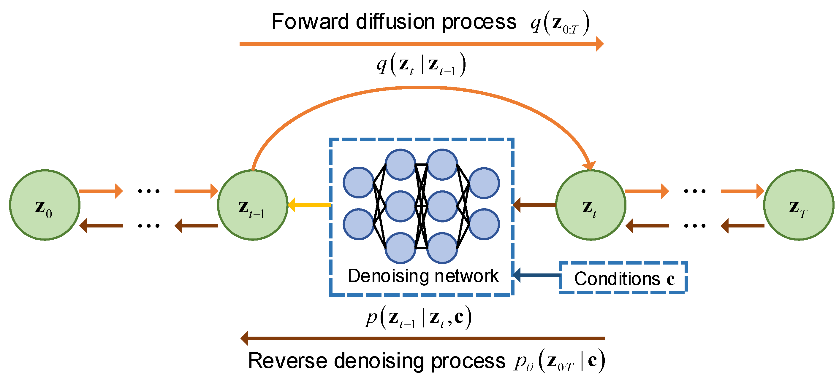
Thus, we introduce the latent space diffusion process illustrated in Figure 3, through using the probabilistic modeling to augment the model’s stability and generalization power [9,10,11,32].

Figure 3. Forward and reverse processes of diffusion probabilistic model.

The diffusion process essentially uses a progressive perturbation to the latent representation, which can be formulated as a Markov chain. In particular, the noise injection process is defined as a Markov chain as

$$q\left({\mathbf{z}}_{1:T}|{\mathbf{z}}_0\right)=\prod _{t=1}^{T}q\left({\mathbf{z}}_t|{\mathbf{z}}_{t-1}\right),$$

(6)

where the single-step diffusion kernel is given by

$$q\left({\mathbf{z}}_t|{\mathbf{z}}_{t-1}\right)=\mathcal{N}\left({\mathbf{z}}_t;\sqrt{1-{\overline{\beta }}_t}{\mathbf{z}}_{t-1},{\beta }_t\mathbf{I}\right).$$

(7)

Next, the closed-form solution for the cumulative diffusion process is expressed as

$${\mathbf{z}}_t=\sqrt{{\overline{\alpha }}_t}{\mathbf{z}}_0+\sqrt{1-{\overline{\alpha }}_t}\mathit{ϵ},\mathit{ϵ}\sim \mathcal{N}\left(\mathbf{0},\mathbf{I}\right),$$

(8)

where ${\alpha }_t\triangleq 1-{\beta }_t$ and ${\overline{\alpha }}_t\triangleq {\prod }_{s=1}^t{\alpha }_s$. By using the cosine scheduling strategy ${\beta }_t=\mathrm{clip}\left(0.5\left(1-cos\left(\pi t/\phantom{\pi tT}T\right)\right),0.999\right)$, we inject noises in the early training stage to enhance the robustness while slowing down the noise accumulation in later stages to preserve the useful information. The reverse denoising process is to learn a parameterized transition kernel, and the parameterized reverse process is defined as

$$p_{\theta }\left({\widehat{\mathbf{z}}}_{0:T}\right)=p\left({\mathbf{z}}_T\right){\prod }_{t=1}^T\left({\mathbf{z}}_{t-1}|{\mathbf{z}}_t\right),$$

(9)

where the reverse transition kernel is

$$p_{\theta }\left({\mathbf{z}}_{t-1}|{\mathbf{z}}_t\right)=\mathcal{N}\left({\mathbf{z}}_{t-1};{\mathit{\mu }}_{\mathit{\theta }}\left({\mathbf{z}}_t,t\right),{\sigma }_t^2\mathbf{I}\right).$$

(10)

In particular, ${\mathit{\mu }}_{\mathit{\theta }}$ is inspired by the score matching theory, which reformulates the denoising task as an estimation of noise component $\mathit{ϵ}$, i.e.,

$${\mathit{\mu }}_{\mathit{\theta }}\left({\mathbf{z}}_t,t\right)={\displaystyle \frac{1}{\sqrt{{\alpha }_t}}}\left({\mathbf{z}}_t-{\displaystyle \frac{{\beta }_t}{\sqrt{1-{\overline{\alpha }}_t}}}{\mathit{ϵ}}_{\mathit{\theta }}\left({\mathbf{z}}_t,t\right)\right),$$

(11)

where the variance is fixed as ${\sigma }_t^2={\displaystyle \frac{1-{\overline{\alpha }}_{t-1}}{1-{\overline{\alpha }}_t}}{\beta }_t$. (11) explicitly sets the training objective of model to the noise prediction, which offers better numerical stability compared to direct mean prediction.

Finally, the noise prediction network is implemented using a multilayer perceptron to approximate ${\mathit{ϵ}}_{\mathit{\theta }}$, i.e.,

$$\begin{array}{cc}\hfill & {\mathbf{h}}_0={\mathbf{z}}_t\oplus \mathrm{Emb}\left(t\right),\hfill \\ \hfill & {\mathbf{h}}_1=\sigma ({\mathbf{W}}_1{\mathbf{h}}_0+{\mathbf{b}}_1),\hfill \\ \hfill & {\mathbf{h}}_2=\sigma ({\mathbf{W}}_2{\mathbf{h}}_1+{\mathbf{b}}_2),\hfill \\ \hfill & {\mathbf{h}}_3=\sigma ({\mathbf{W}}_3{\mathbf{h}}_2+{\mathbf{b}}_3),\hfill \\ \hfill & {\mathit{ϵ}}_{\theta }({\mathbf{z}}_t,t)={\mathbf{W}}_4{\mathbf{h}}_3,\hfill \end{array}$$

(12)

where $\mathrm{Emb}\left(t\right)\in {\mathbb{R}}^{d_e}$ represents the learnable time-step embedding, ⊕ denotes the feature concatenation operation, and $\sigma (·)$ represents the sigmoid activation function, respectively.

Beyond its denoising capability, the diffusion module constructs a smooth and structured latent representation by learning the dominant temporal patterns through iterative noising and denoising. It forces the model to capture stable patterns, e.g., daily periodicity and renewable-related fluctuations, rather than transient spikes or random anomalies. Thus, the latent variable ${\mathbf{z}}_0$ provided to subsequent modules carries cleaner and more representative temporal information.

4.3. Attention Decoder

In this part, the multi-head scaled dot-product attention mechanism is presented first, followed by the GRU updating scheme.

4.3.1. Multi-Head Scaled Dot-Product Attention

The multi-head attention mechanism is incorporated into the decoder to highlight key temporal dependencies in the short-term load forecasting. By learning correlations between different time steps and focusing on multiple representation subspaces simultaneously, the attention module enables the model to capture local variations influenced by external factors and thus improve the prediction precision.

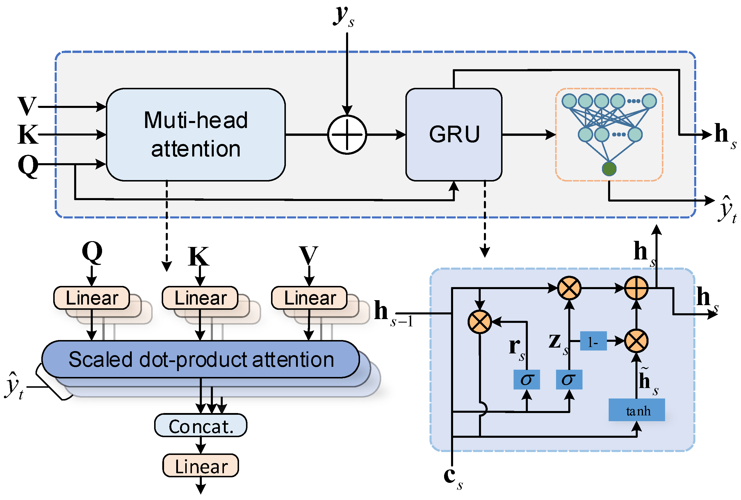
The load sequences of STRLF typically exhibit strong local dependencies and change rapidly. For instance, the load in upcoming hours can be significantly influenced by factors such as weather, temperature and holiday status. To better capture these local dependencies, we introduce the multi-head dot-product attention mechanism as shown in Figure 4, causing the decoder to dynamically focus on the key information from the encoder’s output and thereby improving the prediction accuracy [14,23,33]. The attention mechanism obtains the correlation between $\mathbf{Q}$ (Query), $\mathbf{K}$ (Key) and $\mathbf{V}$ (Value), dynamically assigning weights onto important information. Specifically, during the decoding phase, we use the scaled dot-product attention to achieve the encoder–decoder alignment, defined as

$$\mathrm{Attention}\left(\mathbf{Q},\mathbf{K},\mathbf{V}\right)=\mathrm{Softmax}\left({\displaystyle \frac{\mathbf{Q}{\mathbf{K}}^{\mathrm{T}}}{\sqrt{d_k}}}\right)\mathbf{V},$$

(13)

which is further extended to the multi-head mechanism as

$$\mathrm{MultiHead}\left(\mathbf{Q},\mathbf{K},\mathbf{V}\right)=\mathrm{Concat}\left(\mathrm{hea}{\mathrm{d}}_1,\dots ,\mathrm{hea}{\mathrm{d}}_h\right){\mathbf{W}}^O,$$

(14)

in which each head is expressed as

$$\mathrm{hea}{\mathrm{d}}_i=\mathrm{Attention}\left({\mathbf{QW}}_i^Q,{\mathbf{KW}}_i^K,{\mathbf{VW}}_i^V\right).$$

(15)

The multi-head extension mechanism allows the model to focus on the relevant information in different representation subspaces. In the practical implementation, the head number is set as $h=8$, and the dimension per head is $d_k=d_v=h_{\mathrm{total}}/h$, with $h_{\mathrm{total}}$ as the encoder output dimension.

Figure 4. The attention decoder. The decoder architecture in the figure is based on a multi-head dot-product attention mechanism and a Gated Recurrent Unit. The multi-head attention mechanism dynamically focuses on the key information from the encoder’s output, while the GRU’s adaptive state update mechanism effectively captures the local dependencies and rapid variations in the load sequence.

The attention mechanism further improves prediction accuracy by adaptively highlighting the most relevant temporal positions and external variables. It allows the decoder to selectively focus on critical intervals, e.g., peak-load transitions, sudden PV changes, or battery dispatch events, while suppressing the irrelevant. When combined with the diffusion-generated latent representation, the attention performs a second-stage refinement, i.e., the diffusion suppresses noises at the feature level, and the attention extracts important features at the sequence level. The complementary interaction enables the model to obtain accuracy gains beyond denoising alone.

4.3.2. State Updating of GRU

We next design a GRU-based state updating mechanism that balances the historical and instantaneous information through reset and update gates. By further integrating diffusion outputs and weather features via attention, the decoder can capture local fluctuations while leveraging contextual factors, thereby improving the forecasting robustness and accuracy.

To effectively model local dependencies, we use GRU as the core component of the decoder, as shown in Figure 4. The GRU, by introducing the reset and update gates, enables the adaptive control of historical information and dynamically balances the relationship between local trends and historical records [31]. Its dynamic expressions are as

$${\mathbf{r}}_s=\sigma \left({\mathbf{W}}_r·\left[{\mathbf{h}}_{s-1},{\mathbf{c}}_s\right]+{\mathbf{b}}_r\right),$$

(16)

$${\mathbf{z}}_s=\sigma \left({\mathbf{W}}_z·\left[{\mathbf{h}}_{s-1},{\mathbf{c}}_s\right]+{\mathbf{b}}_z\right),$$

(17)

$${\tilde{\mathbf{h}}}_s=tanh\left({\mathbf{W}}_h\left[{\mathbf{r}}_s\otimes {\mathbf{h}}_{s-1},{\mathbf{c}}_s\right]+{\mathbf{b}}_h\right)$$

(18)

and

$${\mathbf{h}}_s=\left(1-{\mathbf{z}}_s\right)\otimes {\mathbf{h}}_{s-1}+{\mathbf{z}}_s\otimes {\tilde{\mathbf{h}}}_s,$$

(19)

where ${\mathbf{r}}_s$ is the reset gate, ${\mathbf{z}}_s$ is the update gate, ${\tilde{\mathbf{h}}}_s$ is the candidate hidden state, and ${\mathbf{h}}_s$ is the current hidden state, respectively. Specifically, the reset gate ${\mathbf{r}}_s$ determines the contribution of historical information in the current state update. When ${\mathbf{r}}_s$ is close to 0, the model tends to ignore historical information, focusing on the current input and context; when ${\mathbf{r}}_s$ approaches 1, the historical information is fully retained. It is especially suitable for handling abrupt changes in the load sequence. On the other hand, the update gate ${\mathbf{z}}_s$ controls the fusion ratio of new and old states. When ${\mathbf{z}}_s$ is close to 0, the model tends to retain the historical state; when ${\mathbf{z}}_s$ approaches 1, the model assigns the higher attention to present input features. This dynamic adjustment can adaptively balance long-term dependencies and short-term fluctuations. Further, the candidate hidden state ${\tilde{\mathbf{h}}}_s$ integrates the current input and part of historical information, where ${\mathbf{r}}_s\odot {\mathbf{h}}_{s-1}$ represents the historical information filtered by the reset gate, and ${\mathbf{c}}_s$ provides the contextual information of the present time step. The final hidden state ${\mathbf{h}}_s$ is a convex combination of the historical state ${\mathbf{h}}_{s-1}$ and the candidate state ${\tilde{\mathbf{h}}}_s$, integrated as interpolating along the geodesic connecting ${\mathbf{h}}_{s-1}$ and ${\tilde{\mathbf{h}}}_s$ in the hidden state space, with the interpolation weight determined by the update gate ${\mathbf{z}}_s$. The context vector ${\mathbf{c}}_s=[{\mathit{\kappa }}_s,{\mathbf{y}}_s]$ is dynamically aggregated through the multi-head attention mechanism, ${\mathit{\kappa }}_s$ is the output of the multi-layer attention module and the decoder input is ${\mathbf{y}}_s$ at the current temporal step. In particular, the dynamic aggregation of the diffusion module output using the multi-head attention mechanism is expressed as

$${\mathit{\kappa }}_s=\mathrm{MultiHead}\left({\mathbf{h}}_{s-1},{\widehat{\mathbf{z}}}_0,{\widehat{\mathbf{z}}}_0\right),$$

(20)

where the previous time step’s hidden state ${\mathbf{h}}_{s-1}$ is used as the query vector, and the final output ${\mathbf{z}}_T$ of the diffusion module is taken as both the key and value, causing the model to focus on relevant information in different representation subspaces. Further, the decoder receives future weather prediction data ${\mathbf{y}}_s$ corresponding to the load sequence to be predicted at each time step as auxiliary input. The data, obtained from meteorological prediction models or external weather data services, includes key meteorological variables such as temperature and humidity, to fully leverage external environmental factors and optimize the prediction performance.

4.4. Dynamic Weighted Loss

Proposed DATeM needs to optimize two key objectives, i.e., the prediction accuracy and quality of the latent representations. Traditional single loss functions are typically inadequate in balancing these objectives, causing the model to oscillate between overfitting and underfitting. Henceforth, we next propose a dynamic weighted loss function that adaptively adjusts the weights of prediction loss and diffusion loss. This loss function design not only enhances the model’s prediction performance but also improves the robustness of latent representations, thereby providing an efficient and robust framework for the STRLF. Specifically, the tailored dynamic weighted loss function is defined as

$${\mathcal{L}}_{\mathrm{total}}=\lambda {\mathcal{L}}_{\mathrm{MSE}}+\left(1-\lambda \right){\mathcal{L}}_{\mathrm{Diff}},$$

(21)

where ${\mathcal{L}}_{\mathrm{MSE}}$ and ${\mathcal{L}}_{\mathrm{Diff}}$ measure the prediction accuracy and latent representation quality, respectively, and $\lambda$ is the dynamic weight used to balance the contributions of two losses. In particular, the dynamic weight $\lambda$ is defined as

$$\lambda =exp\left(-\gamma ·{\mathcal{L}}_{\mathrm{Diff}}\right),$$

(22)

where $\gamma$ is the sensitivity parameter that controls the magnitude of weights. When the diffusion loss ${\mathcal{L}}_{\mathrm{Diff}}$ is large, it indicates the poor quality of latent representation, and thus $\lambda$ is small, causing the model to focus more on the diffusion loss to improve the robustness. Conversely, when the diffusion loss ${\mathcal{L}}_{\mathrm{Diff}}$ is small (indicating the accurate latent representation), $\lambda$ becomes large, and the model focuses more on the prediction loss to enhance the accuracy. It avoids the tedious manual tuning and allows objectives to be adaptively adjusted during the training, thus significantly improving the model’s generalization ability.

More especially, the prediction loss ${\mathcal{L}}_{\mathrm{MSE}}$ measures the difference between model output and true values, and uses mean squared error (MSE) as the loss function, i.e.,

$${\mathcal{L}}_{\mathrm{MSE}}={\displaystyle \frac{1}{B{S}_y}}\sum _{i=1}^B\sum _{s=1}^{S_y}{\left(y_{i,s}-{\widehat{y}}_{i,s}\right)}^2,$$

(23)

where B is the batch size, representing the sample number in each training step; $S_y$ is the prediction sequence length, indicating the number of future time steps for predicting; $y_{i,s}$ is the true value, representing the load at the s-th time step of the i-th sample, and ${\widehat{y}}_{i,s}$ is the predicted value, representing the model’s forecast for the load at the s-th time step of the i-th sample. The prediction loss is obtained based on the point-wise differences between the model output and true values, directly reflecting the prediction accuracy. Note in the STRLF that the prediction loss aims to capture the local trends and rapid changes in the load sequence, and the diffusion loss ${\mathcal{L}}_{\mathrm{Diff}}$ measures the precision of noise prediction in the diffusion model, using MSE as the loss as

$${\mathcal{L}}_{\mathrm{Diff}}={\displaystyle \frac{1}{BL}}\sum _{i=1}^B\sum _{j=1}^L\sum _{k=1}^h{\left({\mathit{ϵ}}_{i,j,k}-{ϵ}_{\mathit{\theta },i,j,k}\right)}^2,$$

(24)

where L is the sequence length, denoting the number of temporal points within the input sequence; h is the latent representation dimension, representing the feature dimension of encoder output; ${\mathit{ϵ}}_{i,j,k}$ is the true noise, representing the Gaussian noise added at the k-th feature dimension of the j-th time step of the i-th sample; and ${\mathit{ϵ}}_{\theta ,i,j,k}$ is the predicted noise, representing the diffusion model’s prediction of noise at the k-th feature dimension of the j-th time step of the i-th sample, respectively.

4.5. Training Convergence Analysis

In the STRLF, the convergence of the training process directly affects the model’s prediction performance and robustness. Proposed DATeM integrates temporal convolution networks, diffusion probabilistic models and attention mechanisms, with its training designed to ensure efficient and stable convergence. First, the dynamic weighted loss function smooths out gradient fluctuations during the training, thus significantly enhancing the stability of model convergence. In particular, the introduction of diffusion loss imposes an implicit regularization constraint in the latent representation space, which reduces the risk of overfitting. More especially, the dynamic weight adjusts the tradeoff between prediction loss and diffusion loss based on the size of diffusion loss, avoiding the tedious process of manual hyperparameter tuning. Second, the noise injection mechanism of the diffusion process helps the gradient smoothing of the loss function, thereby preventing the gradient explosion or vanishing. By gradually adding Gaussian noises, the diffusion process transforms the original data distribution into a simpler distribution and recovers the original distribution through reverse denoising. The probabilistic modeling approach not only enhances the robustness of latent representation but also significantly reduces gradient fluctuations during the training. Further, the parameter initialization plays a pivotal role in the training convergence.

In particular, we use the Xavier initialization strategy to initialize model parameters, ensure the stable variance of activation values during the forward propagation, and avoids the gradient explosion or vanishing issues. More especially, the weight matrix is initialized as

$$\mathbf{W}\sim \mathcal{N}\left(\mathbf{0},\sqrt{2/\phantom{2\left(d_{in}+d_{out}\right)}\left(d_{\mathrm{in}}+d_{\mathrm{out}}\right)}\mathbf{I}\right),$$

(25)

with the bias term initialized to zero. Finally, a learning rate scheduling strategy is used to further optimize the training convergence. We use a cosine annealing learning rate schedule, dynamically adjusting the learning rate to accelerate convergence. In particular, the learning rate ${\eta }_n$ gradually decays from the maximum value ${\eta }_{max}$ to the minimum value ${\eta }_{min}$ based on the cosine function, i.e.,

$${\eta }_t={\eta }_{min}+{\displaystyle \frac{1}{2}}\left({\eta }_{\max }-{\eta }_{min}\right)\left(1+cos\left(\pi n/\phantom{\pi nN}N\right)\right),$$

(26)

where n represents the current training step and N is the total number of training steps, respectively.

5. Experiments and Results

In this part, the dataset used is first presented, the experiment evaluation metrics are then introduced, and the proposed model is finally contrasted with other baseline forecasting methods.

5.1. Data

The StoreNet dataset originates from the measured data of 20 residential households in the Dingle Peninsula energy community in Ireland, covering minute-level energy and meteorological parameters of the year 2020. It provides a high-resolution, multimodal data foundation for the STRLF [34], recording the energy consumption, photovoltaic generation, battery storage operation and local atmospheric conditions (e.g., temperature, solar radiation, wind speed and rainfall) sampled at a 1 min interval. Its fine-grained characteristics allow the precise capturing of dynamic correlations between load transient fluctuations, sudden weather changes and renewable energy output variability. In particular, the energy sub-dataset includes key indicators such as household energy consumption (Consumption_Wh), photovoltaic generation (Production_Wh), battery charging and discharging (Charge_Wh, Discharge_Wh) and grid interactions (From_grid_Wh, Grid_feed_Wh), as shown in Table 1, which fully characterizes the energy supply-demand dynamics with the integration of distributed energy sources (such as photovoltaics and storage). In addition, the meteorological sub-dataset provides minute-level observations of temperature, solar radiation, wind speed and rainfall, as shown in Table 2. The positive correlation between temperature and cooling/heating demand, along with the direct impact of solar radiation on photovoltaic output, could provide a quantifiable basis for analyzing weather-sensitive load patterns.

Table 1. Feature description of residential load dataset (based on minute-level observation data collected in 2020).

Feature	Description
Date	Timestamps in 1 min intervals (Year 2020)
Production_Wh	Energy generation from PV (Watt-hours)
Consumption_Wh	Energy consumption (Watt-hours)
Charge_Wh	Battery energy storage charging (Watt-hours)
Discharge_Wh	Battery energy storage discharging (Watt-hours)
State-of-charge	Battery state of charge (%)
From grid_Wh	Energy taken from power grid (Watt-hours)
Grid feed_Wh	Energy delivered to power grid (Watt-hours)

Table 2. Feature description of residential meteorological dataset (based on minute-level meteorological observation data collected in 2020).

Feature	Description
Date	Timestamps in 1 min intervals (Year 2020)
Speed	Wind speed (knots)
Dir	Wind direction (degrees)
Drybulb	Drybulb temperature (degrees Celsius)
Cbl	CBL pressure (hPa)
Soltot	Solar radiation (J/cm2)
Rain	Rainfall (mm)

More specifically, the StoreNet dataset is characterized by the proven internal consistency (the Pearson correlation coefficient between power and energy measurements is 1.0), an extremely low data missing rate (with <1% missing values filled using the linear interpolation) and a high degree of alignment with real-world energy community operational scenarios. Its 1 min resolution surpasses the 15–30 min intervals commonly found in similar datasets, making the model better capture transient load fluctuations triggered by weather changes and responses from the energy storage system. Furthermore, the inclusion of battery state-of-charge data provides unique insights into the impact of energy storage buffering on the net load curve, typically absent in traditional residential datasets. Before analyzing, we have to align the energy and meteorological timestamps, aggregate the residential electricity consumption, and perform the seasonal normalization. Note that the dataset stems from an EU-funded demonstration project, and have undergone the strict quality control, validated through the comparison with Ireland standard load curve. Henceforth, the integration of high-resolution, multimodal features and real operational context makes the StoreNet dataset particularly appropriate for prediction models in DER scenarios.

To obtain a trainable dataset for the model, during the data preprocessing, the energy and meteorological timestamps are first aligned, and missing values are imputed through linear interpolation to maintain temporal continuity. A time series splitting strategy is employed, using the first 80% of data for training, the middle 10% for validation, and the final 10% for testing, covering seasonal changes and validating the model’s generalization ability on the unseen data. Let $\mathbf{X}\in {\mathbb{R}}^{B\times L\times d}$ be the input feature matrix, where B is the batch size, L is the historical time window length, and d is the feature dimension. Considering the balance between prediction performance, computational cost and temporal relation, $L=240$ (minutes) is selected, which reflects the load periodicity while ensuring the model’s high prediction accuracy alongside robust training stability and real-time capability. Based on the causal relationships between residential energy systems and the mechanisms governing electricity, alongside the effects of meteorological factors on both electricity consumption and generation, we thus select feature variables exhibiting direct or indirect causal relationships with “load variation”. The features include four types of energy variables (i.e., historical load, photovoltaic output and battery charging/discharging power) and three types of meteorological variables (temperature, solar irradiance and wind speed). Among them, $\mathbf{Battery}\_\mathbf{Power}\left(t\right)=\mathbf{Discharge}\_\mathbf{Wh}\left(t\right)-\mathbf{Charge}\_\mathbf{Wh}\left(t\right)$ are the positive and negative signs of battery discharging and charging, respectively, thereby preserving directional information about energy flow while reducing the feature dimensionality. All features are normalized to improve the training stability, i.e.,

$${\mathbf{X}}_{\mathrm{norm}}={\displaystyle \frac{\mathbf{X}-\mu }{\sigma }},$$

(27)

where $\mu$ and $\sigma$ respectively represent the mean and standard deviation of each feature. The target variable $\mathbf{Y}\in {\mathbb{R}}^{B\times T_s}$ represents the future energy consumption to be predicted, where $T_s$ is the prediction horizon, set to be 30 min, and $Y_{i,s}$ represents the energy consumption value of the i-th sample at future time s. The above design not only captures transient fluctuations in the residential load (e.g., energy storage system charging and discharging responses) but also reflects the long-term effects of weather conditions and renewable energy on load trends.

5.2. Evaluation

To quantify the effectiveness of proposed DATeM, we use some metrics to quantify the prediction accuracy and robustness. Widely used in time series forecasting tasks, these metrics offer insights into the model’s effectiveness in capturing the patterns of residential energy consumption. First, the MAPE reflects the average proportional deviation of predicted results from the true energy consumption values, providing a relative accuracy assessment, defined as

$$\mathrm{MAPE}={\displaystyle \frac{1}{N}}\sum _{i=1}^N\left|{\displaystyle \frac{Y_i-{\widehat{Y}}_i}{Y_i}}\right|,$$

(28)

where $Y_i$ is the actual energy consumption value at time i, ${\widehat{Y}}_i$ is the predicted value at time i, and N is the total number of prediction samples, respectively. MAPE measures the relative magnitude of prediction errors, making comparisons between different datasets or models intuitive. However, when the actual values approach zero, MAPE may lose interpretability. SMAPE is an improved version of MAPE, which reduces the asymmetry of MAPE by considering the absolute errors of both actual and predicted values, defined as

$$\mathrm{SMAPE}={\displaystyle \frac{1}{N}}\sum _{i=1}^N{\displaystyle \frac{|Y_i-{\widehat{Y}}_i|}{\left(\right|Y_i|+|{\widehat{Y}}_i\left|\right)/2}},$$

(29)

which remains effective when actual values approach zero, avoiding the division-by-zero issue occuring in MAPE, and is more robust in cases where the load data is small or fluctuates significantly. In addition, the MAE measures the average absolute deviation between the predicted values and actual energy consumption values, i.e.,

$$\mathrm{MAE}={\displaystyle \frac{1}{N}}\sum _{i=1}^N|Y_i-{\widehat{Y}}_i|,$$

(30)

which provides a direct measure of prediction accuracy, with smaller values indicating the higher prediction accuracy. Note that MAE is particularly suitable for evaluating the average magnitude of prediction errors.

In addition, RMSE is a quadratic scoring rule that measures the average magnitude of prediction errors and assigns higher weights to larger errors, defined as

$$\mathrm{RMSE}=\sqrt{{\displaystyle \frac{1}{N}}{\displaystyle \sum _{i=1}^N}{(Y_i-{\widehat{Y}}_i)}^2}.$$

(31)

Since RMSE is sensitive to outliers, it provides more detailed error information than MAE, particularly in cases where large errors are of particular concerns.

Further, to enhance the comparability of model evaluation, the relative root mean square error (RRSE) normalizes the RMSE, rendering it a scale-independent error metric, defined as

$$\mathrm{RRSE}={\displaystyle \frac{\sqrt{{\displaystyle \sum _{i=1}^N}{(Y_i-{\widehat{Y}}_i)}^2}}{\sqrt{{\displaystyle \sum _{i=1}^N}{(Y_i-\overline{Y})}^2}}},$$

(32)

where $\overline{Y}$ is the mean of actual energy consumption values. In particular, RRSE is appropriate for comparing the model performance across different datasets.

Finally, CORR measures the linear correlation between the predicted and actual values, i.e.,

$$\mathrm{CORR}={\displaystyle \frac{{\displaystyle \sum _{i=1}^N}(Y_i-\overline{Y})({\widehat{Y}}_i-\overline{\widehat{Y}})}{\sqrt{{\displaystyle \sum _{i=1}^N}{(Y_i-\overline{Y})}^2{\displaystyle \sum _{i=1}^N}{({\widehat{Y}}_i-\overline{\widehat{Y}})}^2}}},$$

(33)

where $\overline{Y}$ and $\overline{\widehat{Y}}$ represent the means of the actual and predicted values, respectively. CORR ranges from $[-1,1]$, and values closer to 1 indicate stronger linear correlation between the predictions and actual values. As mentioned above, these metrics complement each other and reflect the model’s prediction performance from different perspectives. MAPE, SMAPE, MAE and RMSE primarily measure the error magnitude, while RRSE and CORR focus on the relative performance and correlation of the model. As such, we ensure the comprehensive evaluation of the proposed DATeM model. The specific hyperparameter settings for the model are summarized in Table 3.

Table 3. Hyperparameter configuration for the model.

Hyperparameter	Value
Historical window length	240
Forecasting window length	30
Batch size	256
Learning Rate	0.0005
Epoch	40
Hidden dimension	64
Diffusion steps	5
GRU Layer	2
Denoising Layer	6

To further provide a fair comparison in terms of computational efficiency, we evaluate the runtime performance of all baseline models under identical hardware and training configurations. Specifically, we measure the total training time required for each model to reach convergence using the same dataset partition, batch size, and optimization settings. This comparison reflects not only the algorithmic complexity but also the practical deployment cost of each method in real residential energy management scenarios. The detailed runtime statistics are summarized in Table 4, which clearly shows the computational differences among the five models.

Table 4. Model runtime comparison.

Model	Average Time
Proposed	55 m 43 s
Proposed w/o attention	54 m 21 s
Proposed w/o diffusion	53 m 17 s
DeepAR [35]	106 m 41 s
TPA [36]	57 m 20 s

As presented in Table 4, the proposed DATeM model achieves a competitive runtime while maintaining significantly higher forecasting accuracy, demonstrating a favorable balance between predictive performance and computational cost.

5.3. Comparison

We then conduct evaluations to verify the superiority of the proposed DATeM model. In particular, the following procedures are listed as follows:

• Experiment setup and dataset partitioning strategy.
• Multi-metric performance comparison with baseline models.
• Statistical significance validation via Friedman test.
• Ablation study analyzing the contributions of key modules.

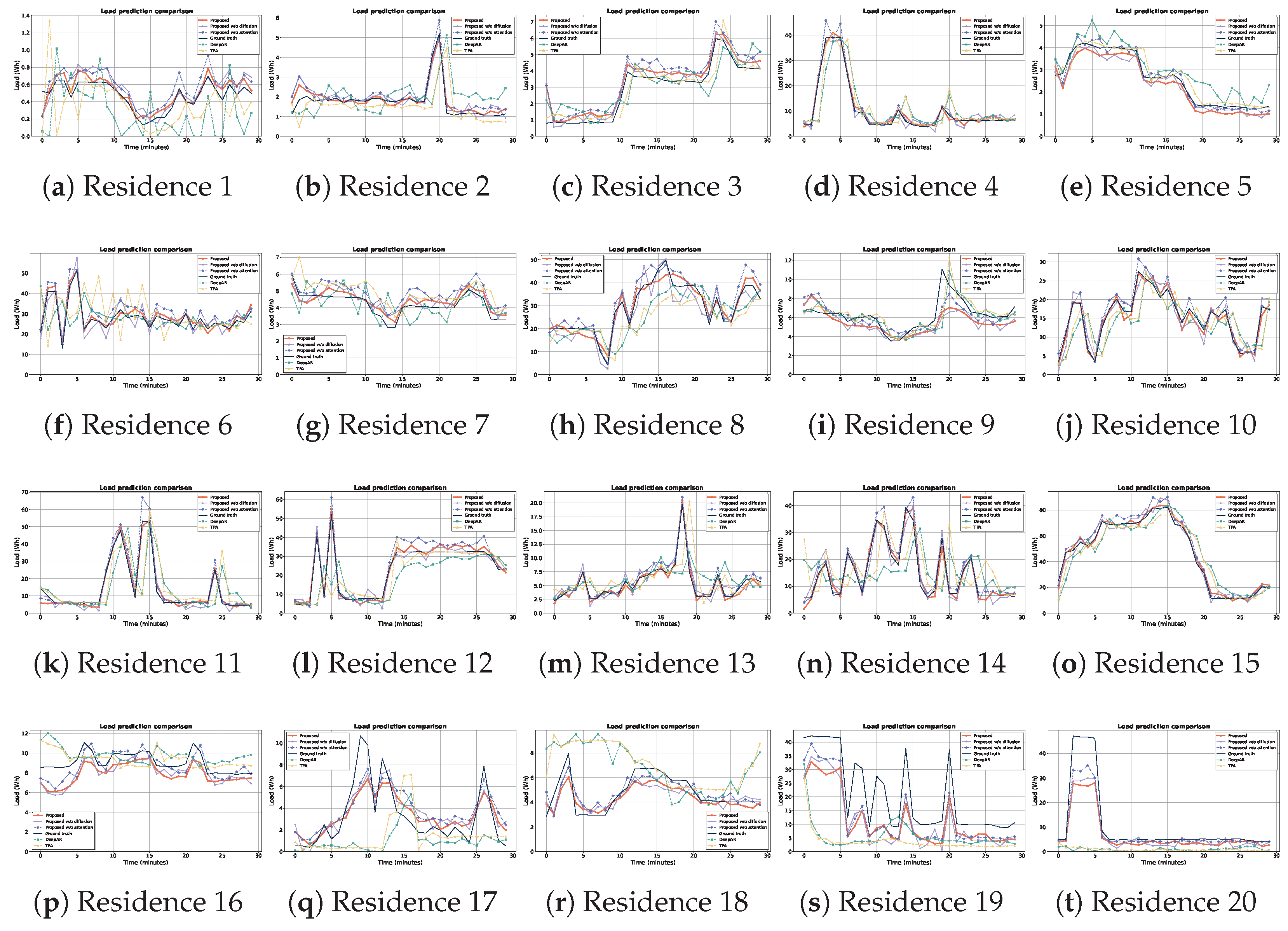
To ensure both comprehensive evaluation and computational efficiency, the 20 residential load datasets are divided into four groups according to seasonal characteristics, with each group containing 5 datasets. In particular, the data is grouped into spring, summer, autumn and winter categories. For the visualized comparison, a representative dataset from each group is randomly selected, as shown in Figure 5, which ensures both the seasonal diversity and experiment objectivity.

Figure 5. Dataset grouping and prediction comparison. Twenty residential load datasets are divided into four seasonal groups (spring, summer, autumn and winter), with five datasets per group. Prediction results are randomly selected to ensure the objectivity and test the model’s robustness across seasons.

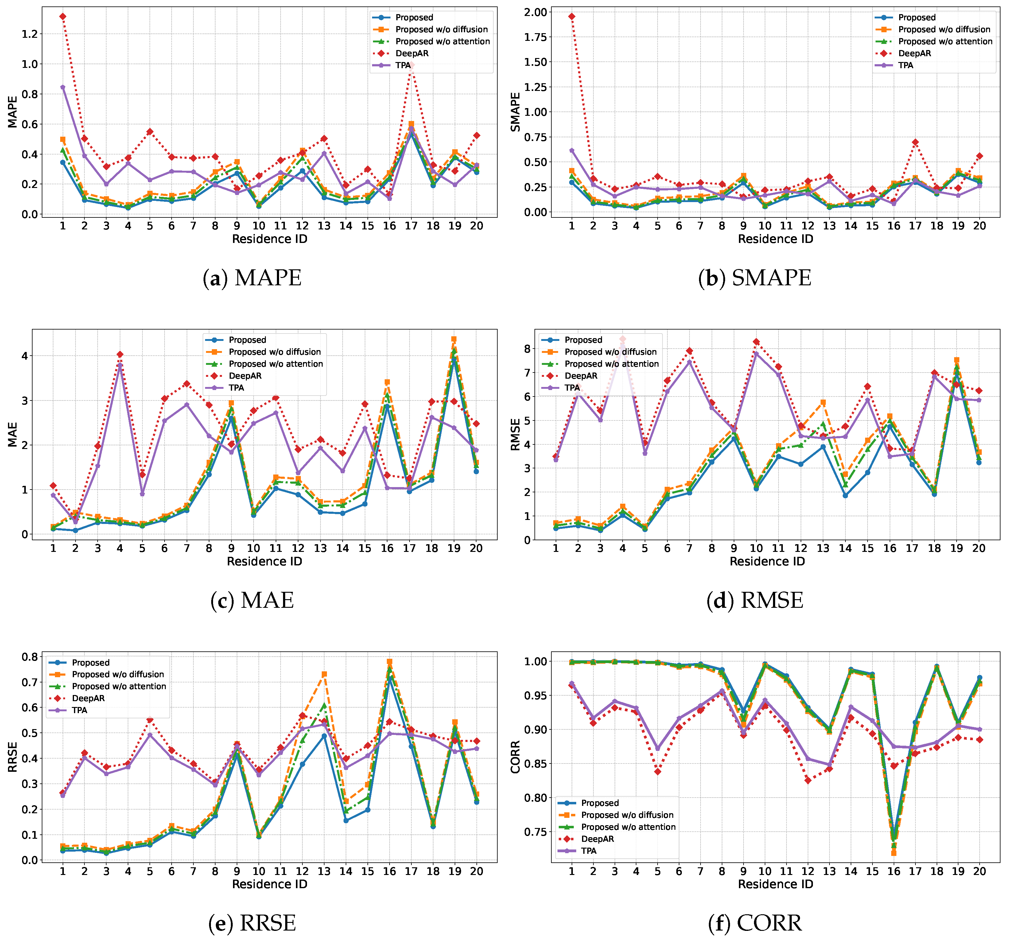
The proposed DATeM model is compared against several strong baselines across six widely adopted evaluation metrics, i.e., MAE, MAPE, SMAPE, RMSE, RRSE and CORR. Figure 6 compares six different metrics across all models for each household. Each curve represents one metric for a given model across different households, illustrating the fluctuation across households. Table 5 shows the values of six evaluation metrics for each model, each of which is averaged over 20 households. As illustrated in Figure 6 and Table 5, DATeM always achieves superior performance across all metrics. In terms of MAE, DATeM attains an average value of 1.0005, substantially outperforming DeepAR (2.2841) and TPA (1.9047). It indicates DATeM’s enhanced sensitivity in capturing fine-grained fluctuations, primarily attributed to the diffusion process’s denoising capability and the TCN encoder’s multi-scale feature extraction. Regarding SMAPE and MAPE, DATeM achieves 0.1589 and 0.1850, respectively, reducing over 57% compared to both DeepAR and TPA. These improvements demonstrate the model’s adaptability under varying load magnitudes and its ability to keep stable predictions even in the presence of seasonal fluctuations and local anomalies. Further, DATeM attains RMSE and RRSE values of 2.5743 and 0.2271, respectively, which are greatly lower than benchmark models. Considering that RMSE would penalize large errors more, the lower RMSE values confirm DATeM’s robustness against abrupt changes and extreme fluctuations, while the lower RRSE values indicate the normalized consistency. The CORR reaches 0.9602, greatly surpassing that of benchmarks. It demonstrates DATeM’s ability in capturing intrinsic temporal structures and long-term dependencies, benefiting from the collaboration between the TCN encoder and attention-augmented GRU decoder.

Figure 6. Performance comparison between proposed DATeM and baseline models. Metrics such as MAPE, SMAPE, MAE, RMSE, RRSE and CORR show that proposed DATeM model significantly outperforms baseline models in the STRLF.

Table 5. Performance evaluation of proposed DATeM against baseline models in the STRLF.

Model	MAE ↓	SMAPE ↓	MAPE ↓	RMSE ↓	RRSE ↓	CORR ↑
Proposed	1.0005	0.1589	0.1850	2.5743	0.2271	0.9602
Proposed w/o diffusion	1.2362	0.2029	0.2414	3.1392	0.2847	0.9543
Proposed w/o attention	1.1413	0.1818	0.2137	2.8925	0.2717	0.9572
DeepAR [35]	2.2841	0.3730	0.4322	5.7948	0.4394	0.8956
TPA [36]	1.9047	0.2220	0.2917	5.4501	0.4123	0.9083

Note: All metrics are calculated on the test set. Arrows indicate the desired direction (↓ lower is better and ↑ higher is better).

In particular, to statistically validate the performance, the Friedman test is further conducted across all households and metrics. As shown in Table 6, DATeM always ranks the highest across all evaluation dimensions, with statistically significant differences ($p<0.000001$) observed among all models. The average ranking of DATeM remains between 1.10 and 1.40, while other models rank much lower. The Friedman test results verify the superior accuracy, stability and generalization ability of DATeM across diverse residential scenarios.

Table 6. Friedman test statistics and average rankings of all models across six evaluation metrics.

	MAE ↓	SMAPE ↓	MAPE ↓	RMSE ↓	RRSE ↓	CORR ↑
Friedman Stat.	44.960	44.120	43.680	52.680	52.680	68.040
p-value	<$1\times {10}^{-6}$	<$1\times {10}^{-6}$	<$1\times {10}^{-6}$	<$1\times {10}^{-6}$	<$1\times {10}^{-6}$	<$1\times {10}^{-6}$
Proposed	1.30	1.40	1.40	1.20	1.20	1.10
Proposed w/o attention	2.45	2.50	2.40	2.30	2.30	2.10
Proposed w/o diffusion	3.45	3.55	3.50	3.45	3.50	3.15
DeepAR [35]	4.45	4.55	4.50	4.55	4.55	4.85
TPA [36]	3.35	3.00	3.20	3.50	3.45	3.80

Note: The values represent average rankings across 20 test datasets. Arrows indicate the desired direction of each metric (↓: lower is better; ↑: higher is better). CORR rankings are computed by reversing the sign of correlation coefficients.

To further understand the contributions of key modules, we conduct ablation experiments by individually removing the diffusion module and attention mechanism. When the diffusion module is removed (i.e., “Proposed w/o diffusion”), the model’s denoising capability substantially declines. The MAE rises to 1.2362 (+23.5%), the RMSE to 3.1392 (+21.9%) and the SMAPE to 0.2029 (+27.6%), while the CORR slightly decreases to 0.9543. As depicted in Figure 5, proposed w/o diffusion exhibits greater local fluctuations and overreactions to transient spikes, particularly during abrupt weather changes or appliance switching. The results verify that the diffusion module plays a critical role in filtering high-frequency disturbances, stabilizing temporal patterns, and enhancing generalization under noisy conditions. In contrast, removing the attention mechanism (“Proposed w/o attention”) incurs a moderate but consistent performance degradation. The MAE increases to 1.1413, RMSE to 2.8925, and MAPE to 0.2137, while CORR decreases slightly to 0.9572. The absence of attention impairs the model’s ability to selectively focus on salient time steps, weakening its responsiveness to local anomalies and rapid load transitions, especially in households with high appliance variability. Consequently, proposed w/o attention struggles to capture short-term dynamics despite retaining the denoising advantage from the diffusion module. Thus, the ablation results demonstrate that both the diffusion module and attention mechanism contribute complementary functionalities. The diffusion module primarily enhances the stability, denoising and resilience under noisy conditions, while the attention mechanism strengthens local temporal discrimination and adaptivity to complex load variations. The integrated design of DATeM enables simultaneous improvements across multiple performance dimensions, showing its effectiveness for the high-resolution and multimodal short-term residential load forecasting.

Although the experiments do not include additional transferability tests, the model inherently supports generalization to unseen households and operating conditions. The diffusion module learns smooth and stable latent structures that reflect universal load behavior patterns, including the daily periodicity, temperature-driven fluctuations, and photovoltaic-related variations. The patterns are common across households, enabling the model to maintain stable performance under distribution shifts. In addition, the attention dynamically adjusts weights based on input sequences, enabling the decoder to focus on critical moments or variables even when encountering unfamiliar load profiles. Together with the scale-insensitive temporal convolution of TCNs, the above advantages empower the DATeM model with robust transfer capabilities for the unseen data.

6. Conclusions

This work has presented an STRLF framework based on generative diffusion models and attention mechanisms, designed to address the complexity, nonlinear dynamics and high uncertainty in the high-resolution load data. By incorporating the diffusion process to enhance the noise robustness, TCN to extract multi-scale temporal features, and attention mechanisms to dynamically focus on key time steps, the proposed DATeM has demonstrated excellent forecasting performance across multiple real residential load datasets. Experiment results have shown that DATeM significantly outperforms existing models in key metrics such as MAE, SMAPE, MAPE, RMSE and CORR, validating its robustness and generalization ability in high-volatility scenarios. In particular, DATeM achieves an average MAE of 1.0005 on 20 residential load datasets, reducing MAE by 56.2% and 47.4% compared to DeepAR and TPA, respectively. SMAPE and MAPE are reduced by 28.4% and 36.6% compared to TPA. In addition, DATeM performs well in RMSE and CORR, further validating its superiority in the high-resolution and multimodal load data. Future works include the improvement of computational efficiency in the diffusion process, the exploration of lightweight models for the real-time prediction, and the extension of DATeM to broader energy forecasting scenarios, e.g., the large-scale grid load.

References

1. Seyedeh, F.; Ravinesh, D.; Mohammad, S.; Mauro, C.; Shahaboddin, S. Computational intelligence approaches for energy load forecasting in smart energy management grids: State of the art, future challenges, and research directions. Energies 2018, 11, 596. [Google Scholar] [CrossRef]
2. Dong, Q.; Huang, R.; Cui, C.; Towey, D.; Zhou, L.; Tian, J.; Wang, J. Short-term electricity-load forecasting by deep learning: A comprehensive survey. Eng. Appl. Artif. Intell. 2025, 154, 110980. [Google Scholar] [CrossRef]
3. Bohara, B.; Fernandez, R.I.; Gollapudi, V.; Li, X. Short-term aggregated residential load forecasting using bilstm and CNN-BiLSTM. In Proceedings of the IEEE International Conference on Innovation and Intelligence for Informatics, Computing, and Technologies (3ICT), Sakheer, Bahrain, 20–21 November 2022; pp. 37–43. [Google Scholar]
4. Sousa, J.C.; Bernardo, H. Benchmarking of load forecasting methods using residential smart meter data. Appl. Sci. 2022, 12, 9844. [Google Scholar] [CrossRef]
5. Paletta, Q.; Hu, A.; Arbod, G.; Lasenby, J. Eclipse: Envisioning cloud induced perturbations in solar energy. Appl. Energy 2022, 326, 119924. [Google Scholar] [CrossRef]
6. Hao, C.H.; Wesseh, P.K.; Wang, J.; Abudu, H.; Dogah, K.E.; Okorie, D.I.; Opoku, E.E.O. Dynamic pricing in consumer-centric electricity markets: A systematic review and thematic analysis. Energy Strateg. Rev. 2024, 52, 101349. [Google Scholar] [CrossRef]
7. Jha, N.; Prashar, D.; Rashid, M.; Gupta, S.K.; Saket, R.K. Electricity load forecasting and feature extraction in smart grid using neural networks. Comput. Electr. Eng. 2021, 96, 107479. [Google Scholar] [CrossRef]
8. Zhou, H.; Zhang, S.; Peng, J.; Zhanga, S.; Li, J.; Xiong, H.; Zhang, W. Informer: Beyond efficient transformer for long sequence time-series forecasting. In Proceedings of the AAAI Conference on Artificial Intelligence, Vancouver, BC, Canada, 2–9 February 2021; pp. 11106–11115. [Google Scholar]
9. Wang, Z.; Wen, Q.; Zhang, C.; Sun, L.; Wang, Y. Diffload: Uncertainty quantification in electrical load forecasting with the diffusion model. IEEE Trans. Power Syst. 2025, 40, 1777–1789. [Google Scholar] [CrossRef]
10. Yang, Y.; Jin, M.; Wen, H.; Zhang, C.; Liang, Y.; Ma, L.; Wang, Y.; Liu, C.; Yang, B.; Xu, Z.; et al. A survey on diffusion models for time series and spatio-temporal data. arXiv 2024, arXiv:2404.18886. [Google Scholar] [CrossRef]
11. Qian, C.; Xu, D.; Zhang, Y.; Bao, J.; Ma, X.; Wu, Z. Residential customer baseline load estimation based on conditional denoising diffusion probabilistic model. In Proceedings of the IEEE International Conference in Power Engineering Applications (ICPEA), Taiyuan, China, 4–5 March 2024; pp. 59–63. [Google Scholar]
12. Zheng, J.; Zhu, J.; Xi, H. Short-term energy consumption prediction of electric vehicle charging station using attentional feature engineering and multi-sequence stacked gated recurrent unit. Comput. Electr. Eng. 2023, 108, 108694. [Google Scholar] [CrossRef]
13. Liu, D.; Lin, X.; Liu, H.; Zhu, J.; Chen, H. A coupled framework for power load forecasting with Gaussian implicit spatio temporal block and attention mechanisms network. Comput. Electr. Eng. 2025, 123, 110263. [Google Scholar] [CrossRef]
14. Feng, Y.; Zhu, J.; Qiu, P.; Zhang, X.; Shuai, C. Short-term power load forecasting based on TCN-BiLSTM-Attention and multi-feature fusion. Arab. J. Sci. Eng. 2024, 50, 5475–5486. [Google Scholar] [CrossRef]
15. Rizi, E.T.; Rastegar, M.; Forootani, A. Power system flexibility analysis using net-load forecasting based on deep learning considering distributed energy sources and electric vehicles. Comput. Electr. Eng. 2024, 117, 109305. [Google Scholar] [CrossRef]
16. Yu, C.N.; Mirowski, P.; Ho, T.K. A sparse coding approach to household electricity demand forecasting in smart grids. IEEE Trans. Smart Grid 2017, 8, 738–748. [Google Scholar] [CrossRef]
17. Stephen, B.; Tang, X.; Harvey, P.R.; Galloway, S.; Jennett, K.I. Incorporating practice theory in sub-profile models for short term aggregated residential load forecasting. IEEE Trans. Smart Grid 2017, 8, 1591–1598. [Google Scholar] [CrossRef]
18. Teeraratkul, T.; O’Neill, D.; Lall, S. Shape-based approach to household electric load curve clustering and prediction. IEEE Trans. Smart Grid 2018, 9, 5196–5206. [Google Scholar] [CrossRef]
19. Xie, G.; Chen, X.; Weng, Y. An integrated Gaussian process modeling framework for residential load prediction. IEEE Trans. Power Syst. 2018, 33, 7238–7248. [Google Scholar] [CrossRef]
20. van der Meer, D.; Shepero, M.; Svensson, A.; Widén, J.; Munkhammar, J. Probabilistic forecasting of electricity consumption, photovoltaic power generation and net demand of an individual building using Gaussian processes. Appl. Energy 2018, 213, 195–207. [Google Scholar] [CrossRef]
21. Lu, J.; Zhang, X.; Sun, W. A real-time adaptive forecasting algorithm for electric power load. In Proceedings of the IEEE/PES Transmission & Distribution Conference & Exposition: Asia and Pacific, Dalian, China, 15–18 August 2005; pp. 1–5. [Google Scholar]
22. Kong, W.; Dong, Z.Y.; Jia, Y.; Hill, D.J.; Xu, Y.; Zhang, Y. Short-term residential load forecasting based on LSTM recurrent neural network. IEEE Trans. Smart Grid 2019, 10, 841–851. [Google Scholar] [CrossRef]
23. Xu, C.; Chen, G.; Zhou, X. Temporal pattern attention-based sequence to sequence model for multistep individual load forecasting. In Proceedings of the IECON 2020 the 46th Annual Conference of the IEEE Industrial Electronics Society, Singapore, 10–21 October 2020; pp. 1710–1714. [Google Scholar]
24. Cheng, L.; Zang, H.; Xu, Y.; Wei, Z.; Sun, G. Probabilistic residential load forecasting based on micrometeorological data and customer consumption pattern. IEEE Trans. Power Syst. 2021, 36, 3762–3775. [Google Scholar] [CrossRef]
25. Zuo, C.; Hu, W. Short-term load forecasting for community battery systems based on temporal convolutional networks. In Proceedings of the IEEE 2nd International Conference on Information Technology, Big Data and Artificial Intelligence (ICIBA), Chongqing, China, 17–19 December 2021; pp. 11–16. [Google Scholar]
26. Lin, W.; Wu, D.; Boulet, B. Spatial-temporal residential short-term load forecasting via graph neural networks. IEEE Trans. Smart Grid 2021, 12, 5373–5384. [Google Scholar] [CrossRef]
27. Tajalli, S.Z.; Kavousi-Fard, A.; Mardaneh, M.; Khosravi, A.; Razavi-Far, R. Uncertainty-aware management of smart grids using cloud-based LSTM-prediction interval. IEEE Trans. Cybern. 2022, 52, 9964–9977. [Google Scholar] [CrossRef] [PubMed]
28. Dab, K.; Nagarsheth, S.H.; Amara, F.; Henao, N.; Agbossou, K.; Dubé, Y. Uncertainty quantification in load forecasting for smart grids using non-parametric statistics. IEEE Access 2024, 12, 138000–138017. [Google Scholar] [CrossRef]
29. Langevin, A.; Cheriet, M.; Gagnon, G. Efficient deep generative model for short-term household load forecasting using non-intrusive load monitoring. Sustain. Energy Grids Netw. 2023, 34, 101006. [Google Scholar] [CrossRef]
30. Khodayar, M.; Wang, J. Probabilistic time-varying parameter identification for load modeling: A deep generative approach. IEEE Trans. Ind. Inform. 2021, 17, 1625–1636. [Google Scholar] [CrossRef]
31. Cho, K.; van Merrienboer, B.; Gulcehre, C.; Bahdanau, D.; Bougares, F.; Schwenk, H.; Bengio, Y. Learning phrase representations using RNN encoder-decoder for statistical machine translation. arXiv 2014, arXiv:1406.1078. [Google Scholar] [CrossRef]
32. Ho, J.; Jain, A.; Abbeel, P. Denoising diffusion probabilistic models. In Proceedings of the 34th International Conference on Neural Information Processing Systems, Virtual, 6–12 December 2020; pp. 6840–6851. [Google Scholar]
33. Vaswani, A.; Shazeer, N.; Parmar, N.; Uszkoreit, J.; Jones, L.; Gomez, A.N.; Kaiser, L.; Polosukhin, I. Attention is all you need. In Proceedings of the 31st International Conference on Neural Information Processing Systems, Los Angeles, CA, USA, 4–9 December 2017; pp. 6000–6010. [Google Scholar]
34. Trivedi, R.; Bahloul, M.; Saif, A.; Patra, S.; Khadem, S. Comprehensive dataset on electrical load profiles for energy community in Ireland. Sci. Data 2024, 11, 621. [Google Scholar] [CrossRef]
35. Cai, S.; Qian, J.; Zhang, Z.; Yu, Y.; Gu, X.; Yang, E. Short-term electrical load forecasting based on the DeepAR algorithm and industry-specific electricity consumption characteristics. In Proceedings of the 2023 7th International Conference on Electrical, Mechanical and Computer Engineering (ICEMCE), Xi’an, China, 20–22 October 2023; pp. 384–387. [Google Scholar]
36. Zhang, X.; Kong, X.; Yan, R.; Liu, Y.; Xia, P.; Sun, X.; Zeng, R.; Li, H. Data-driven cooling, heating and electrical load prediction for building integrated with electric vehicles considering occupant travel behavior. Energy 2023, 264, 126274. [Google Scholar] [CrossRef]
Disclaimer/Publisher’s Note: The statements, opinions and data contained in all publications are solely those of the individual author(s) and contributor(s) and not of MDPI and/or the editor(s). MDPI and/or the editor(s) disclaim responsibility for any injury to people or property resulting from any ideas, methods, instructions or products referred to in the content.
Article Metrics
Citations
Article Access Statistics
Article metric data becomes available approximately 24 hours after publication online.