Abstract
This paper addresses the long-standing question of understanding the origin and evolution of low-frequency unsteadiness interactions associated with shock waves impinging on a turbulent boundary layer in transonic flow (Mach: to ). To that end, high-speed experiments in a blowdown open-channel wind tunnel have been performed across a convergent–divergent nozzle for different expansion ratios (PR = 1.44, 1.6, and 1.81). Quantitative evaluation of the underlying spectral energy content has been obtained by processing time-resolved pressure transducer data and Schlieren images using the following spectral analysis methods: Fast Fourier Transform (FFT), Continuous Wavelet Transform (CWT), as well as coherence and time-lag evaluations. The images demonstrated the presence of increased normal shock-wave impact for PR = 1.44, whereas the latter were linked with increased oblique -foot impact. Hence, significant disparities associated with the overall stability, location, and amplitude of the shock waves, as well as quantitative assertions related to spectral energy segregation, have been inferred. A subsequent detailed spectral analysis revealed the presence of multiple discrete frequency peaks (magnitude and frequency of the peaks increasing with PR), with the lower peaks linked with large-scale shock-wave interactions and higher peaks associated with shear-layer instabilities and turbulence. Wavelet transform using the Morlet function illustrates the presence of varying intermittency, modulation in the temporal and frequency scales for different spectral events, and a pseudo-periodic spectral energy pulsation alternating between two frequency-specific events. Spectral analysis of the pixel densities related to different regions, called spatial FFT, highlights the increased influence of the feedback mechanism and coupled turbulence interactions for higher PR. Collation of the subsequent coherence analysis with the previous results underscores that lower PR is linked with shock-separation dynamics being tightly coupled, whereas at higher PR values, global instabilities, vortex shedding, and high-frequency shear-layer effects govern the overall interactions, redistributing the spectral energy across a wider spectral range. Complementing these experiments, time-resolved numerical simulations based on a transient 3D RANS framework were performed. The simulations successfully reproduced the main features of the shock motion, including the downstream migration of the mean position, the reduction in oscillation amplitude with increasing PR, and the division of the spectra into distinct frequency regions. This confirms that the adopted 3D RANS approach provides a suitable predictive framework for capturing the essential unsteady dynamics of shock–boundary layer interactions across both temporal and spatial scales. This novel combination of synchronized Schlieren imaging with pressure transducer data, followed by application of advanced spectral analysis techniques, FFT, CWT, spatial FFT, coherence analysis, and numerical evaluations, linked image-derived propagation and coherence results directly to wall pressure dynamics, providing critical insights into how PR variation governs the spectral energy content and shock-wave oscillation behavior for nozzles. Thus, for low PR flows dominated by normal shock structure, global instability of the separation zone governs the overall oscillations, whereas higher PR, linked with dominant -foot structure, demonstrates increased feedback from the shear-layer oscillations, separation region breathing, as well as global instabilities. It is envisaged that epistemic understanding related to the spectral dynamics of low-frequency oscillations at different PR values derived from this study could be useful for future nozzle design modifications aimed at achieving optimal nozzle performance. The study could further assist the implementation of appropriate flow control strategies to alleviate these instabilities and improve thrust performance.
1. Introduction
Air and water are essential substances for human life, widely utilized in technology as carriers of energy—whether potential, kinetic, or thermal—for hundreds, if not thousands, of years. While we have a proper understanding of many physical phenomena involving air and water, there is still much to explore. Transonic flows corresponding to high-speed aerospace applications frequently encounter shock waves, whether oblique or normal [1]. One of the most fundamental fluid mechanics phenomena in the aerospace domain, known since 1939 [2], and studied globally for more than 60 years, has been the complex interaction between these shock waves and the underlying boundary layer fluctuations [3,4,5,6]. These interactions, also called the Shock-wave Boundary Layer Interactions (SBLIs), have been established to occur across a wide range of internal and external flow applications [3], including transonic airfoils, supersonic inlets, control surfaces of high-speed aircraft, missile base flows, reaction control jets, over-expanded nozzles, and space launchers [6,7]. The presence of these non-linear interactions [8] leads to several adverse aerodynamic, thermal, and structural impacts clearly emphasized in Refs. [3,4,7,8], warranting the need to critically consider this phenomenon during the design and optimization phase. Owing to the ongoing progress in diagnosis and computational tools [4,9], amelioration of the potentially far-reaching consequences of SBLIs like fluid-flow fluctuations [9], aero-thermal loads [3], as well as buffeting at high angles [10,11] and implementation of flow control techniques [11] have been intensely studied within the academic and industrial sectors.
Interactions associated with SBLIs have been widely studied across various canonical geometries involving shock impingement, ramp flow, transonic flow over a bump, fins, as well as internal flow geometries, including inlets and nozzle flows [4,9]. These investigations primarily followed two methodologies: analysis of mean and unsteady measurements of flow parameters such as static pressure, heat transfer, shear stress, and non-intrusive measurements like Schlieren images, Particle Image Velocimetry (PIV), and many more, unfolding significantly varying flow-field structures across laminar, transition, and turbulent flows [9]. Apart from the incoming flow’s turbulence characteristics, unsteadiness related to SBLIs is further associated with the global instability of these interactions, which further varies between Free Shock Separation (FSS) and a Restricted Shock Separation (RSS) flow. Despite the diverse nature of these canonical flow features, investigations have revealed some common flow attributes associated with SBLIs [6,7,12]. The adverse pressure gradient imposed by the presence of shock waves leads to boundary layer thickening and subsequent separation of the flow. The interaction between shock waves and this boundary layer leads to several unsteady flow characteristics involving a wide range of temporal and spatial interactions. One of the most notable interactions is the origin and propagation of low-frequency unsteadiness appearing as streamwise oscillations of the separation shock [6]. These oscillations involve unsteadiness of the shock wave placed upstream of the recirculation zone, with the shock-wave oscillating at frequencies two to three orders of magnitude lower than the incoming turbulent-boundary-layer fluctuations and the recirculating zone [12,13,14].
The relevance of understanding these unsteady separation flow dynamics in relation to SBLIs for internal flows, including over-expanded nozzles, was emphasized by NASA in their 1996 research announcement [3]. The presence of SBLIs leads to the generation of oscillating -foot shock waves [15,16] over a length called the intermittent region (). The asymmetric structure of this low-frequency oscillating complex flow structure, along with the unsteadiness associated with the boundary layer, mixing layer, and the recirculation zone, leads to the generation of lateral forces, reduction in the output thrust, and degenerated structural integrity. Considering the impact of controlling this flow phenomenon on generating “quieter, shorter, lighter” nozzles [3] for future high-speed applications, a lot of research has been carried out to understand the flow physics related to these low-frequency oscillations [6,8,12,17], especially after the 2001 publication of a review article by Dolling in Ref. [3]. This reinvigorated interest was further supported by the synergistic growth of flow diagnosis tools and computational resources. Much of the earlier investigations made use of the experimental techniques to understand the driving mechanism [13,18,19]. The last decade witnessed the usage of high-fidelity numerical tools like DNS (Direct Numerical Simulations [6,20]) and LESs (Large Eddy Simulations [21]) to explore the phenomenology and obtain further visual insights that were previously not possible with experimental techniques. Notwithstanding these developments, there is a paucity of globally accepted physics governing the driving mechanism behind these large-scale, low-frequency shock pulsations. An analytical study by Plotkin in 1975 [22] inferred these oscillations to be analogous to a random-walk process driven by high-frequency upstream turbulent-boundary-layer fluctuations. Experimental studies carried out by Ganapathisubramani et al. in Ref. [13] indicated the increased influence of upstream low-frequency superstructures on the interaction unsteadiness, which was later contradicted by Piponniau et al. in Ref. [23]. A study carried out by Pirozzoli et al. credited the high-frequency low-scale unsteady interactions to the incoming acoustic feedback mechanism [20].
Despite the plethora of studies indicating the influence of upstream boundary layer momentum on the shock interactions, a number of studies emphasize the increased influence of the downstream driving mechanism. Large Eddy Simulations (LESs) by Touber et al. [24] illustrated that global instability associated with the separation bubble led to contraction and expansion of this separation bubble (“separation-bubble breathing”), which drives these unsteadiness interactions. Piponniau et al. [23] proposed a shear-layer recharge mechanism to be the source of streamwise oscillations. This model proposed the entrainment of separation region flow towards the high velocity shear layer, followed by a recharge feedback mechanism of the separation bubble mass through the reattachment point. This feedback mechanism leads to the large-scale shear-layer “flapping” and separation bubble scaling phenomena. The DNS study of Priebe et al. in 2012 [25] attributed this large-scale shear-layer flapping to near-wall fluctuations that seed the shear layer with appropriate flow structures, leading to unsteadiness of the shear-layer structure. Wu and Martin 2008 [26] presented a unique philosophy entailing an unsteadiness mechanism and proposed that both upstream and downstream flow fluctuations influence the large-scale shock-wave motion unsteadiness, with the former affecting the smaller-scale unsteadiness, whereas separation region pulsation determines the large-scale motions. These conclusions were further corroborated by Piponniau et al. [23] and Priebe et al. [25]. Wu and Martin further established the dependence of shock interaction unsteadiness on the underlying Mach number (), Reynolds number (), and shock incidence angle [27,28,29]. Clemens and Narayanaswamy in Ref. [7] concluded that both the upstream and downstream mechanisms influence the overall unsteadiness, with the former being dominant in the case of strongly separated flows, whereas a combination of the two mechanisms is observed for weak separation flows. Numerical investigations carried out by Touber and Sandham in 2011 [30] utilized Reynolds-Averaged Navier–Stokes (RANS) equations to study these interactions for a shock-reflection configuration and concluded that the large-scale oscillations are associated with the intrinsic properties of the coupled systems, with the upstream and downstream forcing mechanisms not being the only sources of fluctuations. A 2017 LES study segregated the unsteadiness associated with the shock system, separation bubble, and shear-layer interactions into two modes: a medium-frequency mode driven by shear-layer vortices and a low-frequency mode with separation-bubble breathing as the dominant forcing function [31]. Experimental observations compiled by Shanguang et al. [32] concluded that the instability associated with the separation bubble is the greatest source of large-scale shock-wave movement. As an addendum to justifying the relevance of downstream conditions, a Lagrangian framework was developed by Ligrani et al. [14] to post-process time-resolved shadowgraph images for analyzing the coherence of normal shock waves, using pixel-density calculations within different SBLI zones. The detailed coherence, spectral power, and time-lag calculations reinstated the prominent impact of the separation bubble and shear-layer flapping on the unsteadiness interactions. Although a detailed spectral analysis of DNS data presented by Bernardini et al. concluded the increased impact of separation-layer breathing on shock-wave unsteadiness, their results also indicated the influence of many other factors embedded within the shock-wave dynamics [6]. In fact, a doctoral study by Nguyen [33] concluded that apart from the aforementioned local flow features, shock motion related to FSS could be strongly linked to the shape of the exit section. In view of these assertions, it can be stated unequivocally that there is a lack of globally accepted understanding pertaining to large-scale shock-wave oscillations, and hence, requires further scrutiny.
With the increasing demand for high-speed applications [34], there is a need to critically examine the physics related to this phenomenon for nozzle geometry, while ensuing effects related to variation in flow parameters, humidity, as well as nozzle geometry. This internal flow problem is associated with exacerbated flow complexities due to multiple reflected shock-wave generation, separation in multiple regions, mixing layers, recirculation, and their interactions [16,35]. Notably, flow through an over-expanded transonic De Laval nozzle at elevated back pressure involves a supersonic-to-subsonic flow transition through shock-wave generation, increased flow separation together with shock-wave oscillations. These shock waves in the divergent section interact with the turbulent boundary layer, leading to complex asymmetric shock-wave oscillations. Several attempts have been made in the past to enhance understanding related to low-frequency oscillations (LFOs) within the context of high-speed flow through nozzles. Under the auspices of NASA Glenn Research Center, a 2009–2010 study by Johnson et al. made use of experimental campaigns to contemplate the complex multiple-shock-wave structure dynamics [35] and sources of instability related to LFO [36]. These studies recognized that separation strength, shear-layer instability, and asymmetric shock-wave structure had a prominent impact on the shock motion. Inferences drawn from a later LES numerical study by Olson and Lele [37] were found to be in concordance with Johnson et al.’s experimental observations [36]. A numerical study by Martelli et al. [38] reasoned that the self-sustaining shock-wave oscillations were related to the pressure differential between the downstream re-compression region and the nozzle exit (ambient).
In view of the above, the principal point of contention in this field is the ubiquitous lack of consensus related to the source of these shock-wave oscillations across all canonical problems, especially nozzle flows. Moreover, the research gap associated with fundamental understanding related to shock-wave oscillations within open flow separation interactions [7] linked with over-expanded nozzles further warranted the need for this research. Increased understanding related to these low-frequency shock-wave oscillations within nozzle configurations, while deliberating its dependence on the overall flow conditions and geometry, could pave the way for future technological advancements in nozzle design optimization. Insights associated with the underlying spectral energy distribution and transfer mechanisms of low-frequency oscillations at different pressure ratios would be helpful in implementing design modifications to the current state-of-the-art by making use of adaptive nozzle design or flow control strategies, aimed at curtailing the peak instabilities. Although significant progress has been made through experimental campaigns and high-fidelity simulations such as DNS and LES, these approaches are often constrained by technical limitations, high computational costs, or difficulties in accessing certain flow regions. As a result, there remains a clear need for modeling frameworks that can systematically explore parametric variations and what-if scenarios that are either impractical or prohibitively expensive to examine experimentally. In this regard, simplified but validated numerical approaches, particularly unsteady Reynolds-averaged Navier–Stokes (URANS) formulations, offer a pragmatic compromise. While not as detailed as DNS or LES, URANS-based models have shown the potential to reproduce essential flow features of SBLIs, including low-frequency unsteadiness. When benchmarked against experimental datasets, these models can provide valuable insights into the relative influence of upstream turbulence, coherent flow structures, and downstream separation bubble dynamics. In nozzle applications, this capability is particularly relevant, as the complex interaction of multiple shocks, recirculation zones, and asymmetric flow separation makes experimental isolation of individual mechanisms difficult. In view of the same, the experimental observations will be collated with results obtained using a numerically efficient URANS framework and capture low-frequency oscillations in over-expanded nozzle flows. While representing only an initial step towards more comprehensive modeling, the approach covered in this paper demonstrates that simplified models, when carefully validated, can complement experimental diagnostics and provide predictive understanding necessary for aerodynamic optimization and potential flow-control strategies in high-speed propulsion systems. Comprehensions on the physical principles inferred through this experimentally and numerically obtained spectral energy distribution and coherence estimates would also be helpful for advancement in other fluid dynamic systems, such as multiphase or chemical reactive flows. Furthermore, the ensuing unique combination of advanced spectral analysis, coherence, and time-lag estimations backed up by numerical evaluations, provides a critical step forward in spectral energy analysis of shock-wave oscillations. The integration of this causal framework with machine learning techniques like the one implemented by Hu et al. [39] and Kumar et al. in [40] provides a concrete and cutting-edge methodological exemplar for potential future research directions arising from the present work.
To that end, the current research aims to process, analyze, and evaluate the dynamic shock-wave oscillations within an asymmetric convergent–divergent nozzle operating at transonic speeds and enhance understanding related to the linked low-frequency unsteadiness. The research objectives are listed hereafter:
- Setting up an experimental setup to investigate shock-wave–boundary layer interactions and low-frequency shock-wave oscillations, allowing for systematic variation of parameters such as pressure ratio, humidity, nozzle expansion rate, and channel geometry.
- Establishing a synchronized experimental evaluation of a time-resolved large dataset of plan-view high-speed Schlieren images and pressure transducer readings, followed by preliminary numerical evaluations.
- Formulating a new analysis framework for such complex problems involving the collation of advanced spectral analysis using Fast Fourier Transform (FFT), wavelet transform [6] and coherence estimation [14] to comprehend the unsteady parameters linked with LFO within the context of FSS [12,15,16] of nozzle flow dynamics.
- Integrating high-fidelity computational techniques like URANS with spectral techniques and experimental evaluations to further enhance physical insights related to the coupled SBLIs.
- It was envisaged that the appropriate correlation of these results, carried out at different pressure ratios, would increase understanding related to spectral energy evolution and distribution, thereby helping create novel designs or flow-control strategies to improve thrust performance.
The current paper makes use of the following sections to analyze the flow physics of SBLIs. Section 2 provides details about the experimental and numerical set-up, including the deliberated flow conditions, implemented measurement systems, and the procedure(s) thereof. Section 3 corresponds to the results and discussion section, making use of time-resolved Schlieren images and pressure data to understand the governing flow physics. This section culminates in providing a brief overview of the numerical simulations carried out to capture the flow unsteadiness and underlying flow structure. The terminal section, that is, Section 4, presents some key conclusions drawn out from these experimental and numerical investigations.
Despite numerous studies on shock-wave oscillations in over-expanded nozzle flows, a clear consensus on the underlying physical mechanisms governing their low-frequency unsteadiness is still lacking. The present study addresses this research gap by employing a combination of experimental investigations and a validated numerical technique framework carried out at different PRs to systematically investigate the spectral energy distribution, coherence, and causal interactions governing low-frequency shock-wave oscillations in nozzle configurations. By integrating advanced spectral and time-lag analyses with experimental observations, this work aims to elucidate the energy transfer mechanisms governing these oscillations. The inferences will not only advance the fundamental understanding of shock-induced flow separation dynamics but also provide a foundation for future adaptive nozzle designs and flow control strategies, targeting stability enhancement in high-speed propulsion systems.
2. Methodology
2.1. Experimental Setup and Procedure
The laboratory located on the air test rig of the Department of Power Engineering and Turbomachinery of the Silesian University of Technology (SUT) was used to perform the experimental tests presented in this paper. This lab has been extensively engaged in carrying out state-of-the-art experimental investigations on nozzle flows [41,42] for many years. Tests in the current research were performed using the air vacuum experimental setup installed at SUT for analysis of high-speed aerodynamic flows (Figure 1). A schematic of the utilized experimental setup is presented in Figure 1d, whereas the components indicated in the schematic are described in Table 1. The blowdown experimental setup makes use of a Roots blower to maintain the required pressure in the gas chamber placed downstream of the inlet pipe, regulated by control valves to maintain the required PR. To make sure that stabilization and repeatability of inlet conditions are maintained across the experiments, a temperature–pressure-stabilized inlet chamber is installed upstream of the test section. The presented method of regulation ensures convenient, precise, and repeatable setting of the PR at which the stand operates. Apart from this, the setup makes use of triple measurement of the mass flow parameters using hot-wire anemometers upstream, downstream, and within the test section, to ensure a uniform and accurate determination of the flow characteristics related to the tested geometry. This also helps in detecting potential external leaks during the experiments.

Figure 1.
(a) Air vacuum experimental setup overview; (b) Test section consisting of the tested De Laval nozzle; (c) Schlieren visualization setup; (d) Schematic of the air vacuum system installed at SUT.

Table 1.
Components of the air vacuum system at SUT.
The test section size constrained by the maximum possible flow-rate (up to 0.2 kg/s) is fitted with a convergent–divergent De Laval planar nozzle to carry out the required flow measurements. Geometry related to the tested nozzle geometry and the fluid domain is notated in the top and front views presented in Figure 2a. This nozzle is a circular nozzle placed midway between the test sections. Dimensions related to the nozzle and domain geometry indicated in Figure 2a are provided in Table 2.
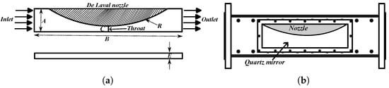
Figure 2.
(a) Nozzle profile and fluid domain specifications; (b) Test section.
Table 2.
Tested nozzle dimensions.
In order to support clear flow-field visualization across the visible and UV wavelength frequencies, the test section is fitted with a quartz shield (Figure 2b).
The experimental procedure was initiated by opening the motor-controlled valves (2, 3) to suck the ambient air through the inlet pipes (1), which were stored within the pressure chamber (5) meant for stabilizing the flow. The cut-off valve (4) meant to direct flow towards another test section was closed for the current experiments. Air from the pressure chamber was further directed towards the Roots blower (7) through the cut-off valve (6). The roots chamber further pumped the air towards the test section. Through the usage of a bypass duct and control valves (8–9), flow rate was regulated across the test section, leading to varied nozzle PR values across the nozzle. Beyond this, a temperature chamber (T) was used to maintain the desired temperature and humidity using a control valve (10). This air was further directed towards the test section (12) using the control valve (11). For testing, the bypass valve directed towards the test section was opened. This flow was maintained till fluctuations related to inlet flow parameters like pressure and temperature obtained a stable value. After the flow settled, a one-second window was selected to acquire the final data used for processing.
2.2. Experimental Measurement System
Two sets of measurement systems were installed while carrying out the experiments. The first system was used to measure the parameters related to the inlet conditions in order to ensure safe and repeatable operation of the stand. The second measurement system carried out measurements related to the nozzle flow. Data acquisition across the two systems was achieved using National Instruments’ NI/PXI-6255 module, which was connected to a measuring cluster. This cluster consisted of impulse tubes and screened cables connected to appropriate sensors and transducers to carry out the measurement of various flow parameters. Pressure measurement pertaining to the nozzle flow was accomplished using a series of pressure transducers (P1–P30) placed on the wall, as shown in Figure 3. The measurement system also consisted of three analog high-frequency pressure transducers (>10 kHz), synchronized with the Schlieren setup to capture in-sync instantaneous pressure and image data. The first high-frequency transducer, notated as P1AC, was placed close to the throat, P2AC was placed within the converging section, whereas P3AC was placed within the diverging section near the nozzle outlet (depicted in Figure 3).

Figure 3.
Pressure transducer ports for pressure measurement.
Considering the concurrence of shock-wave motion detection through Schlieren imagery and fast-response pressure measurements, as emphasized by Combs et al. in Ref. [43]), the current study implemented the basic knife-edge Schlieren technique to detect the density gradients associated with shock-wave oscillations [44]. The Schlieren setup presented in Figure 1c utilizes a pair of high focal length (200 cm) lenses (for increased sensitivity), a high-intensity–homogeneous LED spot illuminator, and a high-speed PHANTOM camera capable of recording videos at frame rates up to 100 thousand frames per second. The setup during the current study captured the frames at 6000 frames per second. The synchronized camera–illuminator system made use of a High Dynamic Range technique to appropriately measure changes in density, as well as light intensity variations within the flow.
The Schlieren technique relies on the deflection of point source light ( and ) across the knife edge. This deflection is dependent on the change in refractive index (n), which is further a function of density variation [44], as shown in Equation (1).
Here, L is the length along the optical axis, is the refractive index of the surrounding medium, and x, y are the axes along which a value is measured. The aforementioned light deflections ( and ) appear as varying gray-scale intensities across the Schlieren frame. Schlieren images for individual PR cases were obtained at 6000 frames per second, with each test spanning a duration of 1000 ms.
Data obtained from the Schlieren setup and actuators (described above) were managed using an in-house LabVIEW program. Subsequent to this preliminary data acquisition and manipulation stage, further processing of the data was carried out in MATLAB® Version 24.2 [45] to obtain the required shock-wave position and frequency spectrum plots.
2.3. Flow Conditions
As mentioned above, experimental studies were carried out for three different PRs. Specifications related to the three cases are listed in Table 3.
Table 3.
Investigated flow conditions.
Here, and are the total pressure and total temperature, whereas and are the test section outlet values, respectively. Ambient relative humidity was measured at ≈28% during these experiments. The variable PR was accomplished by varying the mass flow rate within the chamber, leading to higher PRs for increased mass flow rates. In order to represent a particular PR plot, results pertaining to the three PR cases will be represented as PR1.44, PR1.6, and PR1.81, respectively. Surface smoothness was achieved through appropriate surface machining and grinding, leading to minimal roughness, warranting minimal influence of roughness on the overall flow interactions. Further details regarding the measurement uncertainties associated with pressure and humidity measurements are provided in [41].
2.4. Digital Image Processing of Schlieren Frames
The Schlieren setup recorded a one-second plan-view video for the three cases. This video was sampled at 6000 frames/s (sampling rate: ) and processed using an in-house MATLAB® script to extract the location of the shock-wave front (which is also called the inviscid shock-wave component or Mach disk). Since the location of this primary shock wave determines the location of the entire shock-wave structure [46], it was assumed that understanding the unsteadiness related to its position would capture the low-frequency oscillations related to SBLIs, as elaborated earlier in Ref. [47].
The overall process of carrying out this detection is described in Figure 4, implemented using the image processing toolbox in MATLAB version 2024b. This process is initiated by converting the video into digitized frames captured at an interval of μs, in the form of time-resolved RGB matrices. These RGB images are converted into grayscale images. Shock waves are defined by thin lines of steep pressure or density gradients. The presence of these steep gradients is displayed as a sequence of bright and dark regions [17] in Schlieren images, leading to the formation of unequivocal pixel gradient lines within the frames. The implemented code aimed to detect these lines through the usage of an appropriate edge detection technique. However, before applying the required image segmentation, the frames were pre-processed to remove noise and carry out image contrast enhancement. This stage involved convolution of the images with high-frequency filters, leading to enhancement of edges, followed by contrast enhancement to make the shock-wave edges more prominent. The images were further moderately smoothed using a Gaussian filter (standard deviation, ) technique to suppress fine noise pixels within these images. Through these steps, shock-wave edges in the frames were enhanced, leading to an efficient shock-wave detection code.
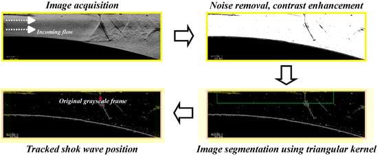
Figure 4.
Flow-chart to carry out digital image processing of Schlieren images to detect shock-wave position. Green box in the bottom-right image is a small pre-determined sliding rectangular kernel, wherein the segmentation was carried out to detect the position of shock waves.
In order to detect the location of these shock-wave edges, image segmentation using the Canny algorithm [48] was carried out. This has been utilized previously in numerous shock tracking investigations [47,49], due to their robustness and effectiveness in capturing abrupt changes in pixel intensity. In order to neglect the outlier edges detected within the segmented image, a sliding window-based shock detection method is utilized, wherein a small sliding rectangular kernel is applied across a predefined portion of the image to identify regions with maximum summed pixel values. The portion corresponding to the maximum summed pixel values is labeled as the location of the Mach disk. In order to avoid spurious edge detection, the kernel was moved only within the rectangular portion specified in Figure 4. This method is robust to noise, adaptable, and effective even if the shock-wave edges are not sharp. The shock-wave position obtained using the implemented technique was further processed to obtain the mean position of the shock wave with respect to the throat, which was further non-dimensionalized using the throat height. The mean shock-wave position was further used to normalize the time-resolved shock-wave position about the mean position. This normalized shock-wave position data and digitized time-resolved Schlieren images were further processed using spectral analysis tools described henceforth, to discern the underlying spectrum and correlation dynamics pertaining to different interaction regions. A brief uncertainty analysis on image-based shock-wave position data emphasized an uncertainty of less than , establishing the accuracy of the employed technique to capture the shock-wave position.
2.5. Spectral Analysis of Pressure Data and Shock-Position Data
FFT has been a preferred methodology to carry out unsteadiness analysis across several disciplines since 1965 [50], including spectral segregation with respect to SBLIs [7,14]. This method involves deciphering the magnitudes of dominant overtones within the flow unsteadiness by parlaying the time-resolved signal into discrete frequency amplitudes. To that end, this paper made use of FFT to evaluate the square root power spectra of the individual waves embedded in the signal as a function of frequency in the form of frequency spectrum and power-spectral density (PSD) plots. In the first stage, time-resolved pressure data were converted into the respective frequency spectrum plots. Further details regarding the adopted methodology can be gleaned from Ref. [17]. This process has been repeated for the three PR cases to provide an overview of how the dominant tones shift and vary with different PR values.
In a later section, FFT was implemented on shock-wave position data for the three PR cases to derive the pertinent PSD distribution plots. This was followed by a smoothing operation to identify the associated prominent frequency peaks. The averaging was carried out by using a variable moving average scheme across the spectrum, as listed in Table 4. The symbol represents the Nyquist frequency, which is Hz, and is the frequency resolution, which is 1 Hz.
Table 4.
Smoothening operation for PSD data obtained using shock-wave position data.
2.6. Spectral Analysis Using Wavelet Transform of Pressure Data
The spectral content from FFT analysis of a signal is a time-averaged overview of the underlying frequency spectrum [6]. Due to the underlying time-averaging of the localized features, FFT leads to the loss of critical temporal information about the underlying flow features localized in time. Its output could be considered to present an accurate picture of the associated frequency spectrum, if the flow is stationary or ergodically periodic, measured over a long time. However, flow related to SBLIs is complex and characterized by multi-scale, non-stationary fluctuations, and thus warrants the need to carry out spectral analysis that provides frequency segregation of the flow signature, as well as temporal evolution of these components. One such method being used across several applications [51], including SBLIs [6,32], is the Continuous Wavelet Transform (CWT). Due to its temporal resolution feature, CWT provides the ability to capture intermittency, as well as time-stamped modulation of the complex flow-field signal, providing a microscopic overview of the features involved.
The wavelet transform of a time-varying signal g(t) is given by:
where , , and are the mother function, wavelet scale, and time-translation parameters, respectively. The mother function is scaled and time-translated along the signal to enable visualization of the amplitude of different frequency components and also present the time evolution of these features. Further information regarding the process and elements involved can be gleaned by the readers from Ref. [52]. In a nutshell, the process involves convolving the narrow temporal window data with mother function variants generated by scaling in frequency and shifting in the time domain, and hence extracting the associated time-evolving frequency spectra. Out of the plethora of wavelets, the current paper makes use of the complex Morlet function, which is a time-limited modulation of a sinusoidal function with a Gaussian envelope [32], described in Equation (3).
where is the non-dimensional frequency. The Morlet transform has been attributed to produce arbitrarily high resolution in frequency, as well as the temporal domain, compared to other mother functions [6,51]. This mathematical tool was used to derive the time-evolving spectral plot of pressure data. The output from such a transformation is presented later as excerpts of the scalogram contour distribution plots in Section 3.5, wherein individual scalogram plots were derived by calculating the modulus of the Morlet transform, . Comparison of the individual scalogram plots will provide insights into the time evolution and spectral variation of underlying flow interactions located at different regions within the flow.
2.7. Spectral Analysis of Interaction Regions: Spatial FFT
Spectral analysis of the pressure data and shock-wave position data described heretofore provided an overview of unsteadiness associated with the global shock system. However, given the non-homogeneous characteristic of SBLIs, spectral analysis of pixel densities associated with the different regions, namely, separation region, upstream boundary layer, downstream boundary layer (beyond the reflection shock), separation shock, and Mach disk, would be imperative to capture the energy distribution between different interaction regions. Thus, time-sequence Schlieren images were extracted and processed to evaluate PSD pertaining to different regions for the three PR cases. This analysis, carried out using MATLAB version 2024b, implemented the Welch’s method [53] to carry out the spectral evaluations.
This process involved the selection of a particular image, followed by the selection of pixel points within the region being analyzed. The time-resolved grayscale values at these selected points are filtered using a low-pass fifth-order Butterworth filter with a cut-off frequency of 1 Hz less than to remove high-frequency noise, as well as the DC component within the pixel signals. This pixel-specific time-stamped filtered signal is further transformed into PSD using the windowed FFT method [53]. This windowed FFT made use of 1200 samples per segment, followed by the usage of a Hamming window to avoid spectral leakage. This windowed FFT leads to a reduction of random noise components while providing a smoother PSD plot at the expense of relatively lower-frequency resolution (5 Hz). The individual FFT plots are averaged for the different sets of FFT plots at every frequency. Analogous to PSD data pertaining to shock-position data discussed in Section 2.5, the averaged FFT data in this analysis was also smoothed using a variable moving average scheme elaborated in Table 5. This process of deliberating FFT plots associated with different spatial regions within the flow has been coined as ‘spatial FFT’.
Table 5.
Smoothening operation for PSD obtained using time-resolved pixel data at different region-specific pixel locations.
This process was repeated for five different pixel locations placed in close proximity to each other for a specific region. The output of averaged PSD plots from these pixel locations was ensemble-averaged to determine the overall PSD plot corresponding to different regions of the interaction. In the study, five pixels were selected on an image for a specific region. The time-resolved pixel intensities on these points were further divided into 9 segments, leading to the evaluation of 9 individual spectra for each pixel. Thus, a total of 45 individual spectra were calculated for a specific region. These 45 sets of PSD data were ensemble-averaged to determine the final PSD plot. This method leads to improved signal-to-noise ratio, especially in the regions of maximum density gradients like shock-wave structure, separation bubble, etc.
2.8. Coherence and Time-Lag Analysis of Pixel Intensities Corresponding to Different Regions
Coherence is a measure of correlation between two distinct signals as a function of frequency, and magnitude-squared coherence is a measure of this coherence. For instance, magnitude-squared coherence () values between time-sequence pixel intensities pertaining to regions and will be computed by Equations (4)–(6).
In these equations, is the cross power spectral density, and are the power spectral densities of the two signals, whereas is the square of magnitude spectrum at different frequencies within the frequency domain. The output of these equations is a set of values at different frequencies. A higher value of is indicative of increased correlation between the two signals at a specific frequency.
Another measure of correlation between two signals is termed the time lag (). A positive is indicative of value occurring before . It is calculated as follows:
where is the phase lag between the two signals at a specific frequency. This phase lag was calculated using the real and imaginary components of at different frequencies.
In the current numerical setup, these quantities have been evaluated by comparing time-resolved pixel intensities corresponding to inviscid normal-shock-wave location, downstream boundary-layer (downstream BL) pixels, downstream -foot pixels, upstream boundary-layer pixel (upstream BL) values, and separation-region pixel values. The identifiers corresponding to different regions are illustrated in Figure 5.

Figure 5.
Different interaction zones being explicitly analyzed for spectral distribution and correlation analysis.
Coherence and time lags pertaining to comparison between different regions were identified using the variables (Equation (4)), and (Equation (7)), respectively, with and being identifiers for the regions being compared, as shown in Figure 5. For instance, coherence and time lag between the shock-wave-region pixel (denoted by alphabet a) and downstream-boundary-layer pixel (denoted by alphabet b) values will be denoted as and , respectively. The complete process of estimating coherence and time-lag values, implemented through in-built MATLAB functions, is as follows: five pixel values from the respective regions indicated in Figure 5 were selected, time-sequence pixel intensities for the five pairs of signals were filtered using a fifth-order Butterworth filter, and saved as vectors. Magnitude-squared coherence and time-lag values were evaluated for every pair of pixels from the two regions. These five pairs of values were subsequently ensemble-averaged and smoothed to find the final set of coherence and time-lag values.
2.9. Numerical Methodology and Simulation Setup
To complement the experimental investigations of low-frequency oscillations, spectral signatures, and coherence of shock–boundary-layer interactions, a set of transient numerical simulations was carried out. While the experimental campaign provides direct access to time-resolved pressure signals, Schlieren imagery, and their spectral decomposition across frequency and spatial domains, numerical modeling offers a controlled framework for interrogating the underlying flow physics under identical operating conditions. In particular, the numerical simulations serve two objectives: first, to assess whether a computationally efficient RANS-based formulation can capture the large-scale unsteadiness observed experimentally; and second, to provide additional insight into flow-field quantities, thereby strengthening the interpretation of spectral analysis, wavelet decomposition, and coherence evaluations. Within this context, ANSYS Fluent 2024 [54] was employed to solve the three-dimensional, compressible Navier–Stokes equations within the Reynolds-Averaged (RANS) approach [55] for the nozzle configuration under consideration, with the modeling details summarized as follows.
The governing equations of continuity, momentum, and energy were spatially discretized using the finite volume method and solved using the pressure-based coupled algorithm, which simultaneously resolves pressure and velocity fields. To ensure stable pressure–velocity coupling on collocated grids, the Rhie–Chow momentum interpolation method [56] was employed, which constructs face velocities using a momentum-based correction to avoid checkerboarding artifacts and enhance numerical stability. Air was modeled as an ideal gas, with density computed from the equation of state, establishing a coupling between pressure and temperature. Convective terms in the density, momentum, and energy equations were discretized using the second-order upwind scheme, while the turbulence transport equations for turbulent kinetic energy (k) and specific dissipation rate () were discretized using the QUICK (Quadratic Upstream Interpolation for Convective Kinematics) scheme [57]. QUICK offers third-order spatial accuracy on structured meshes by blending central differencing and upwind biasing, improving gradient resolution while limiting numerical diffusion. Turbulence was modeled using the shear stress transport (SST) variant of the k– model [58], with the turbulence equations solved in a segregated fashion, independently from the coupled system of flow equations. Temporal discretization employed a bounded second-order implicit formulation to enhance accuracy and maintain stability in unsteady simulations. Molecular viscosity was held constant throughout the calculation.
A structured, multi-block mesh was generated using ANSYS Mesher to discretize the computational domain. The mesh is divided into three distinct zones: an inlet section, a central channel region, and an outlet section, as shown in Figure 6a. The entire mesh consists exclusively of hexahedral cells to maintain high numerical accuracy and low numerical diffusion, particularly important for resolving flow gradients in compressible regimes. The mesh is static (non-adaptive) and remains unchanged throughout the simulation. The central channel block, which encompasses the separation point and the Mach disk formation region, was refined to provide higher spatial resolution where flow features are most sensitive. A close-up of this section can be seen in Figure 6b. This refinement is symmetrically applied both upstream and downstream of the neck—the narrowest section of the geometry—to accurately resolve shock interactions, expansion waves, and flow instabilities. The structured topology supports the use of high-order spatial discretization schemes, further enhancing solution fidelity in critical areas. In the wall-normal direction, a structured boundary layer mesh is implemented along the entire channel region; its cross-section is shown in Figure 6c. The boundary layer consists of five hexahedral layers confined within a 1 mm wall-normal distance, and the first cell height adjacent to the wall is 75 μm. Although the boundary layer mesh was designed to provide some near-wall resolution, the preliminary mesh configuration results in a non-dimensional wall distance of approximately in the channel region. This coarser mesh was used in the early stages of the study to explore qualitative flow behavior and identify dominant flow features. For near-wall turbulence treatment, wall function based on correlation was employed, which allows for reasonable modeling accuracy even when the first cell lies in the buffer layer or lower log-layer. Despite the relatively coarse resolution near the wall, the simulations yielded promising results, capturing key flow structures and oscillatory phenomena consistent with expected characteristics, thereby validating the mesh for initial investigative purposes.

Figure 6.
(a) Overview of the structured multi-block mesh discretizing the computational domain, including the inlet (left), central channel region (middle), and outlet extension (right). Velocity vectors are shown at the inlet (blue arrows) and outlet (red arrows) boundaries to indicate flow direction. (b) Close-up view of the refined mesh in the central channel region near the narrowest section (neck), highlighting the hexahedral cell distribution optimized for resolving shock and flow features. (c) Cross-sectional view of the structured boundary layer mesh along the channel wall, showing the five hexahedral layers with the first cell height of 75 μm, designed for near-wall turbulence resolution.
A circular pressure inlet boundary condition was applied at the upstream end of the computational domain. The inlet, with a diameter of 0.15 m, is located 0.2 m upstream from the channel entrance and forms the base of a cylindrical extension that connects to the main channel. This upstream extension was introduced to allow the inflow to develop properly and to prevent the artificial influence of the boundary condition on the flow inside the channel. At the downstream end of the channel, a similar cylindrical extension is attached, serving as the outlet region. All surfaces of this outlet cylinder—except the one where the channel exits—are defined as pressure outlet boundaries. This configuration minimizes backflow or reflection effects at the outlet, ensuring that the downstream boundary does not adversely influence the internal flow within the channel. The static pressure and temperature values prescribed at the inlet boundary were carefully set to replicate the conditions experimentally measured at the entrance of the channel for the three pressure ratios investigated. This approach ensures that both the thermodynamic and flow conditions entering the domain closely resemble those observed in the physical experiments, thereby improving the fidelity and relevance of the numerical results. Similarly, the outlet boundary conditions, including static pressure and temperature, were assigned to match the corresponding experimental measurements, minimizing artificial reflections and ensuring a physically consistent flow development through the domain.
3. Results and Discussion
3.1. Analysis of Pressure and Mach Number Variation Within the Nozzle
Plots in Figure 7a illustrate the variation of static pressure (P) along the nozzle length for the three PR cases. The three plots demonstrate the presence of a “classic” trend associated with nozzle flow comprising expansion, sudden shock compression, and recovery [35]. The expansion occurs within the converging section, as well as some distance beyond the throat. However, due to the presence of overexpansion, shock waves are generated within the diverging section for all the cases, leading to a sudden increase in the P value between ports P17 and P22. It can also be seen that as PR increases, pressure measured at port P1 increases. This leads to P being higher for increased PR within the entire converging section. It can also be seen that the generation of shock-wave compression for the higher PR occurs at a later distance from the throat. This leads to the generation of a steeper pressure gradient for higher PR, which would further indicate the presence of increased flow separation for higher PR, leading to increased impact of flow separation on the shock-wave structure. The plot pertaining to PR1.81 demonstrates the presence of two spikes in p values, leading to the presence of two humps. This is characteristic of a -foot shock structure [59]. Due to the increased separation shock intensity for higher PR, the flow downstream of the first shock remains supersonic, leading to the development of expansion fans and compression shocks. Due to this, the pressure recovery is delayed significantly for higher PR. However, beyond these bumps, the value of P starts recovering. The convergence of p values at for all three cases, despite differences in the downstream compression shock position and the delayed onset of pressure recovery for higher PR, further indicates that a higher PR results in a stronger adverse pressure gradient, leading to increased flow separation intensity. This increased flow separation instability feeds the complex SBLI dynamics.
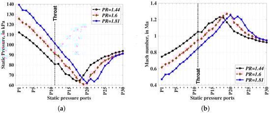
Figure 7.
Averaged streamwise variation of flow parameters for varying PR: (a) Static pressure variation, (b) Mach number variation.
Plots in Figure 7b present the Ma variation along the nozzle for three cases. These values were calculated by applying isentropic relations to the aforementioned p values. The value of Ma associated with the three cases increases within the converging section and up to a finite distance downstream of the throat, beyond which it starts to reduce due to the formation of shock waves, and ultimately converges to similar values at port P30. Ma reduction is steeper and occurs at a lower Ma for lower PR values, as they are dominated by inviscid normal shock-wave phenomena resulting in a steeper flow deceleration. It is also noticeable that the higher PR amounts to higher Ma values within the nozzle, followed by a slower deceleration beyond the shock wave. The higher amounts to increased bulk momentum of the incoming flow, which has a significant impact on the origin of SBLIs, and hence the underlying unsteady interactions. The presence of two bumps for PR1.81 is again indicative of an increased impact of the separation shock, leading to the formation of oblique shocks, and hence the gradual shock-induced deceleration.
3.2. Schlieren Image-Based Flow Structure Analysis of Nozzle Flow for Different Pressure Ratios
In order to shed more light on the large-scale oscillations of shock waves, this section presents a preliminary analysis of the comparison of the flow structure corresponding to the three wind tunnel conditions. This is achieved by comparing the time-sequence Schlieren images at four successive time samples ( to , where is the sampling rate of the images). The subfigures in Figure 8 illustrate the presence of varying SBLI dynamics leading to discrete Mach disk lengths, the -foot structure, and the accompanying flow separation region and coherent vortical structures linked thereto, which is on par with the physics elaborated in [46,59,60]. It was also noted that this complex shock-wave structure presented streamwise oscillations within the divergent section. The aim of this research was to carry out spectral characterization of these different events and enhance fundamental understanding related to these low-frequency shock-wave oscillations. As noted in the figures, shock-wave structures consist of an inviscid normal shock (also called the Mach disk) near the top surface (indicated as A in Figure 8b), a prominent -foot shock structure (indicated as B) comprising a leading separation shock (bright white line: C, Figure 8c) and a reflection wave (downstream dark line: D) linked with the lower region followed by shear-layer separation region (E). The two shock waves (C and D) merge with the Mach disk at the triple point (F). The varying intensities of these shock-wave structures lead to varying flow separation dynamics downstream.

Figure 8.
Time-sequence Schlieren images for different cases (a,d,g,j) PR; (b,e,h,k) PR; (c,f,i,l) PR. Dotted red ellipses are regions of interest.
The time-sequence images for PR1.44, that is, Figure 8a,d,g,j, indicate that the lower ratio leads to SBLIs being dominated by the inviscid Mach disk structure occurring closer to the throat. This led to increased and earlier pressure increment beyond the shock wave for PR1.44, as indicated earlier in Figure 7a. Owing to the thinner boundary layer at this portion, as well as the weaker shock wave, the effect pertaining to the shock-wave impinging on the boundary layer is minimal, and hence the -foot structure is visibly small-scale. It was also contemplated from the time-sequence images that this normal shock wave was more stable. Thus, the weaker shock wave at this PR leads to a more stable shock wave [12]. Due to the presence of this normal shock wave, downstream flow is dominated by subsonic flow aerodynamics and forms a fully separated shear-layer downstream. Due to the relatively lower velocity gradient between the shear layer and the post-shock core flow, density variations leading to Kelvin–Helmhotz (KH) instabilities are less intense, resulting in minimal density fluctuations downstream of the shock. The flow downstream is mainly dominated by non-linearities associated with shear-layer eddies. Notwithstanding these attributes, this case still presented streamwise oscillations of the shock-wave structure.
As PR increases to , this flow interaction becomes more complex, and the time-resolved images illustrate the presence of incipient separation [61], leading to the formation of FSS, wherein the flow downstream of the shock wave close to the surfaces lacks flow reattachment [15], and a prominent -foot structure originates. Due to the increased energy of higher PR flow, the shock wave originates at a later distance (Figure 8b) downstream of the throat, wherein the attached boundary layer is thicker. These observations are similar to the ones observed by Papamoschou [35]. Higher PR leads to increased momentum of the incoming flow, which results in a fuller profile, leading to a more downstream position of the SBLIs [7]. Furthermore, higher PR leads to the development of a stronger shock wave, resulting in an increased adverse pressure gradient that interacts with the underlying boundary layer to create a separation bubble upstream of the Mach disk that ultimately results in the formation of an oblique separation shock. The flow downstream of this oblique wave interacts with the shear layer. Due to the heightened velocity differences between these two regions, KH instability fluctuations are more intense in this case (Figure 8e: F). Figure 8e further indicates the origin of an additional stronger shock wave from the triple point, downstream of the separation shock, called the reflection shock (G). Its intensity increases as flow develops with time (compare Figure 8e: G and Figure 8h: H). This leads to increased KH interactions at the foot of the -foot structure. Moreover, Figure 8k shows the presence of a white line originating from the triple point, called the slip line (I), which is a result of slow-moving flow downstream of the normal shock interacting with the faster flow downstream of the reflection shock leading to increased flow intermixing, and hence the intense density variations appear as line originating at the triple point. Distance between the first separation shock and the trailing reflection shock is called the separation length scale [7] and is notated as . Notably, the shear-layer separation is exacerbated for this case, leading to increased density fluctuations downstream. Moreover, flapping of the shear layer was more appreciable at this PR.
As PR increased to PR1.81, -shock-wave intensity increased and occurred at a later distance from the throat. Due to the overall shock-wave intensity increment, flow separation downstream of the Mach disk is exacerbated, leading to increased interactions and the -foot structure becoming more intense. In fact, Figure 8c,f,i,l illustrate the presence of a small -structure even at the upper portion of the whole structure (See J in Figure 8i). Fluctuations pertaining to were observed to be more significant at this PR, which would indicate increased oscillations within the separation region, as well as global instability associated with vortex shedding. This subsequently leads to a more intense reflection shock for this case. Thus, increased PR led to increased interactions between the different regions related to SBLIs, which would indicate the increased influence of high-frequency KH instabilities associated with mixing between the core supersonic flow and shear layer, as well as the eddies associated with slip line formation (See K in Figure 8i,l). The increased flow interactions are corroborated by the presence of increased density fluctuations downstream of the separation shock for PR1.81. The increased influence of turbulent eddies on the overall flow pattern would indicate the presence of increased impact of high-frequency turbulent eddies on the frequency spectrum, which will be further emphasized using spectral analysis in a later section. Similarly to PR1.44, this case also exhibited the presence of low-frequency large-scale oscillations of the shock-wave structure with respect to the separation-shock foot. In a nutshell, the higher the PR, the more prominent the impact of separation and reflection shocks will be, leading to a more prominent shock-wave structure. An illustration depicting the evolution of flow structure as PR increases within the studied nozzle is provided in the schematics presented in Figure 9. The lower PR (Figure 9a) flow was dominated by normal shock component occurring at an earlier position within the nozzle, whereas the higher PR flow is dominated by a more complex -foot shock structure emanating at a latter distance, leading to increased flow inter-mixing, and hence a more complex downstream flow structure, including reflected shocks, slip lines, increased shear-layer separation and KH vortices.

Figure 9.
Schematic to illustrate the evolution of shock-wave structure as PR increases; (a) Flow structure at lower PR; (b) Flow structure at higher PR.
Thus, we can say that increasing the PR led to increased interactions between the different components, leading to a significant impact on the overall structure of these SBLIs. Moreover, these heightened complex interactions between the shock wave and underlying boundary layer led to the formation of shock trains (L in Figure 8l), a bigger separation region (M in Figure 8l), increased flapping of the shear layer (N), as well as increased vortices downstream of the shock wave, as indicated by the O region in Figure 8l. Large-scale low-frequency oscillations associated with nozzle flows were established for all the cases. In order to provide critical insights into these quasi-periodic oscillations and reconcile the causes of this unsteadiness, a detailed spectral analysis was carried out, which is illustrated in the following sections.
3.3. Spectral Analysis of Pressure Data Obtained Using High-Frequency Transducers
Critical understanding regarding the aforementioned unsteadiness was initiated by comparing the FFT plots of time-sequence pressure data obtained using the high-frequency transducers P1AC (Figure 10a) and P3AC (Figure 10b), with the former being closer to the throat, and the latter being further downstream of the throat (See Figure 3) and placed on the upper wall. An experimental study carried out by Bourgoing et al. [62] demonstrated the presence of similar frequency peaks across the upper and lower ends of an asymmetric wave. Moreover, it is well established that reflected shock waves generate an upward deflection of flow [6], which is the reason why shear layer and prominent -foot reflections on the lower surface will be measured by transducers placed on the opposite wall. Thus, deductions drawn from the spectral analysis of transducers placed on the upper wall will also be qualitatively similar to the lower surface flow. Through a succinct analysis of the underlying frequency components, FFT analysis leads to enhanced understanding related to oscillations that contribute significantly to the global energy spectra of unsteadiness interactions contained within the time-domain signals of pressure transducer data. Considering the number of samples being 6000 and a sampling rate () of 6000 per second, the resolution in the frequency domain was 1 Hz. As per the Nyquist criterion, the maximum frequency discernible through this sampling was , that is, 3 kHz. Considering the placement of transducers on the top-surface, the spectral plots obtained using the transducer data would be dependent on the fluctuations due to Mach disk gradient, shock-wave location, as well as reflected fluctuation from the lower surface interactions.

Figure 10.
Spectral power distribution for pressure data fluctuations at different pressure ratios at different locations (a) P1AC (b) P3AC.
For the three PR cases, Figure 10a shows that P1AC detects the presence of three distinct peaks associated with pressure oscillations and a fourth small pulsating peak between 985 and 1068 Hz. A 2020 experiment on the compression corner by Shanguang et al. demonstrated the presence of similar three peaks residing between 100 to 1000 Hz, which provides further context to the validity of these results. The first frequency peak lies between 242 and 293 Hz, the second between 501 and 569 Hz, and the third between 814 and 933 Hz. These ranges will be termed as frequency band −1 (FB1), frequency band −2 (FB2), and frequency band −3 (FB3), respectively. The most dominant frequency, which resides within the range of 500–600 Hz, is in concordance with the 0.4 kHz–2 kHz range, as estimated by Brusniak & Dolling, 1994 [63]. It is also evident that the corresponding frequency and power of these peaks increase significantly between PR1.44 and PR1.6. However, as the PR changes from 1.6 to 1.81, this frequency increment is markedly lower. In fact, the peak frequency value for FB1 reduces from PR1.6 to PR1.81. It was noted earlier that the flow associated with PR1.44 is dominated by the inviscid normal shock-wave structure, whereas the latter two were associated with increased separation shock impact leading to increased impact of the oblique shocks on the overall flow structure. Normal shock leads to exacerbated adverse pressure gradient conditions, amounting to a heightened scale of the associated vortices, which amounts to lower-frequency oscillations. The flow corresponding to -foot interactions is associated with smaller-scale oscillations, leading to higher-frequency turbulence flow eddies. Owing to the diverse nature of the underlying flow physics, frequency differences between the former two cases are significantly steep. On the other hand, the flow structure related to PR1.6 and PR1.81 is similar, leading to mitigated differences between their respective peak frequency values. The subtle increment in frequency value between PR1.6 and PR1.81 for FB2 and FB3 is attributed to increased bulk momentum, leading to increased incoming turbulence, and hence a higher frequency [26]. Peaks pertaining to FB4 are presented only for PIAC. This would indicate the presence of a localized driving mechanism related to FB4 oscillations. The close proximity of shock waves to P1AC could lead to acoustic reflection, small-scale vortices, or small-scale flapping of the shear layer, which are associated with high-frequency oscillations. Considering the dependence of these phenomena on the incoming flow momentum, higher PR amounts to a significantly increased frequency value of peaks associated with FB4.
It is also noticeable that the overall magnitude of FB2, FB3, and FB4 increases between PR1.44 and PR1.6, whereas it reduces from PR1.6 to PR1.81. This could be associated with the relative placement of the transducer with respect to the shock-wave interaction. As mentioned earlier, the complex interaction region moves downstream as PR increases. The transition from PR1.4 to PR1.6 leads to a shock wave moving closer to the P1AC, leading to increased magnitudes of the detected FB2, FB3, and FB4 peak oscillations. On the other hand, between PR1.6 and PR1.81, the interaction regions move further downstream. The reduced magnitude indicates that the transducer moves upstream at some of the time-stamps, leading to a reduction of the averaged magnitude of these pulsations. The magnitude related to FB1 increases between PR1.44 and PR1.6, whereas it remains similar in magnitude between PR1.6 and PR1.81. This indicates the presence of a low-frequency large-scale phenomenon within the flow, for which the amplitude varies significantly between the first two, whereas it remains the same between the last two cases. This indicates that this modulation is related to large-scale instabilities within the separated shear layer that lead to flapping of the shear layers [64], which could be related to the shedding of vortices and separation-layer breathing. At higher PR, this global instability increases, leading to an elevated scale of separation-layer oscillations, and hence the lowered-frequency value of the associated FB1 peak. Thus, transducer data placed closer to the throat, wherein the effect of shock-wave unsteadiness would be the maximum, illustrates the presence of three primary peaks, which will be further corroborated using shock-wave position data FFT. The plots also demonstrate that as the effect of -foot increases, small-scale oscillations associated with broadband frequency pulsations become more prominent, and are showcased as increased high-frequency spectrum magnitudes. Therefore, higher PR values imply a greater impact of flow separation, which results in a broader and more attenuated oscillation spectrum.
Spectral plots pertaining to port P3AC in Figure 10b display unique characteristics pertaining to pressure wave oscillations. The pressure waves recorded at this location will be influenced by large-scale streamwise oscillations of shock waves, small-scale high-frequency turbulent oscillations related to flow separation, shear layer, as well as acoustic disturbances. Frequencies pertaining to the first three peaks occur at the same frequency value compared to those existing at P1AC. This is indicative of increased correlation of the associated oscillations across the two locations. It is also noteworthy that the magnitude of FB1 and FB2 peaks is lower at P3AC compared to P1AC. Thus, downstream of the shock, increased mixing due to separation-induced SBLIs leads to attenuated power of these two modes of oscillations, which is indicative of their association with the overall interaction dynamics. It is also noteworthy that the amplitude of FB1 increases as PR increases, which provides further credence to this modulation being associated with the separation-induced vortex shedding phenomena (to be clarified using wavelet analysis in a later section). The amplitude of FB3 is higher at this location. Thus, the effect of high-frequency oscillations is higher at this location, which would indicate the dependence of these oscillations on the shear-layer oscillations, including flapping, which becomes more intense and thicker as the flow moves downstream of the interaction region [64]. Thus, the impact of high-frequency overtones attributed to mixing-layer flow eddies present at this location increases, leading to increased frequency and amplitude scales. These observations emphasize the relation of low-frequency peaks with large-scale oscillations of the interactions, whereas the higher-frequency peaks were related to the turbulence characteristics linked with incoming turbulence or the shear-layer separation dynamics. Notably, these revelations are similar to those observed by Pirozolli et al. in [65], wherein similar assertions were drawn for flow across an impinging shock configuration.
The FFT plots demonstrate the presence of multiple spectral peaks ranging between 240 to 990 Hz, with a lower power value within the diverging section. The lower two peaks are indicated to be related to the overall shock structure interaction and their oscillations, whereas the third and fourth peaks are indicative of their relation with the shear-layer instabilities. The plots also demonstrate the presence of increased correlation between the pressure data at the throat and diverging section, which is indicative of dependence of the downstream fluctuations on the throat location. To gain further insights into these unsteadiness events, detailed spectral analysis of shock-wave position data, as well as interaction regions, has been carried out in the succeeding sections.
3.4. Spectral and Statistical Analysis of Shock-Wave Position Data Derived Using Lagrangian Approach
Spectrum plots obtained using pressure data are constrained by the fact that it does not represent the complete flow-field, leading only to an external overview of the underlying unsteadiness [3]. In order to increase the validity of these plots and also increase understanding related to shock-wave dynamics, Figure 11 plots the spectral power density () of the frequency spectrum derived by carrying out an FFT of the non-dimensionalized shock-wave position with respect to the mean position of the shock wave. Data pertaining to the shock-wave position was obtained using the image processing technique described earlier in Section 2.4. The acquired FFT plot was further smoothed using the variable moving average technique described earlier in Section 2.5. However, moving average parameters were adjusted to improve clarity of the plots pertaining to this data and are described in Table 6.
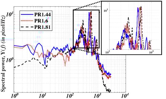
Figure 11.
Spectral power density for the quasi-periodic shock-wave position about the mean shock-wave position obtained using Fast Fourier Transform.
Table 6.
Smoothening operation for PSD obtained for time-resolved shock-wave position data.
It can be seen that most of the spectral power pertaining to oscillations associated with shock-wave position data resides within 173 Hz to 1000 Hz, with powers reducing above and below these frequencies. Analogous to the FFT plot pertaining to pressure fluctuations described above, these plots also display the presence of three prominent frequency peaks for the three cases, with frequency values lying within the same range as that mentioned earlier. The first band (FB1) lies within 242 Hz to 297 Hz, the second (FB2) within 485–580 Hz, and the third one (FB3) within 767–920 Hz (See Table 7). Moreover, similar to pressure FFT plots, the frequency value of these peaks is commensurate with the PR value, with a higher PR leading to a higher-frequency value. This increment is higher at ≈14% within PR1.44 to PR1.6, which reduces to an increment of 6.1% between PR1.6 and PR1.81. It can be ascertained that the frequency range estimated by the pressure data, as well as shock-wave position data, is very close to each other, which provides validity to the presence of these three primary oscillations dominating the entire flow field. Furthermore, this provides credibility to the accuracy of the employed Schlieren images to capture the overall flow unsteadiness.
Table 7.
Peak frequencies pertaining to dominant oscillations for the three PR cases.
Given the increased impact of flow-field parameters, including upstream and downstream conditions, on shock-wave position, spectral plots pertaining to shock-wave position data indicate the presence of many more low-amplitude frequency peaks, which were not visible within the pressure data FFT. The FFT plot pertaining to PR1.44 illustrates the presence of an additional peak at 8 Hz and several small peaks below 100 Hz, which are not visible in the other two cases. The predominant normal shock interaction leading to mitigated flow separation for PR 1.44 increases the influence of upstream flow turbulence [7] on the shock-wave position. Considering the emphasized role of upstream high-frequency flow in driving low-frequency oscillations [24], the detected low-frequency peaks could be attributed to the upstream-boundary-layer unsteadiness that results in a subtle ‘breathing effect’, causing small shifts in the shock location that are too subtle to be detected by the transducers. This will be further corroborated using the statistical analysis of amplitude related to these oscillations in a later analysis, as well as coherence and spatial FFT analysis. Notably, the power of oscillations below the range of FB1 is significantly lower for higher PR cases, further indicating the increased impact of high-frequency turbulent eddies and high-frequency shear-layer unsteadiness on the overall shock-wave flow oscillations.
The shock-wave position data were further processed to obtain imperative statistical data related to these oscillations. The bar plots corresponding to the mean (), minimum (), and maximum () positions of the detected shock wave from the throat have been discussed in this study. These values have been non-dimensionalized using the throat diameter and notated as . As noted in Figure 12a, increases as PR increases owing to the increased bulk momentum of the incoming flow field, leading to convection of SBLIs in the downstream direction [22]. This is further corroborated by the presence of a smaller upstream value of the shock-wave position () for lower PR. The value of shock-wave position also presents similar trends between PR1.6 and PR1.81. However, PR1.44 presents a higher value compared to PR1.61. Due to the extended spatial range of the shock-wave position for higher PR, relative to the throat, standard deviation () also subtly increases for higher PR (Figure 12b). Paradoxically, the non-dimensionalized amplitude of oscillations () about the mean position of the shock wave demonstrates a lower value as PR increases (Figure 12c). This reduction in amplitude is in line with the established literature [16]. For PR1.44, the flow is dominated by the inviscid normal shock-wave component, leading to a more stable compression, while oscillating with higher amplitudes, which further leads to a deeper downstream position of the shock wave (Figure 12a). On the other hand, for higher PR flow, the presence of -foot structure amounts to improved feedback between the various interaction regions, leading to a more unstable shock-wave structure, and hence smaller . The distinction associated with a stark difference between the parameters related to PR1.4 and PR1.6, compared to the subdued variation between PR1.6 against PR1.81, was discerned from the FFT plots of shock-wave position data also. This is again associated with the increased influence of separation bubble pulsation for PR1.6 and PR1.81, which was significantly lower for PR1.44. Thus, PR variation impacts the overall convective and feedback forcing functions related to SBLIs, leading to varied flow interactions and, hence, the oscillations. To enhance understanding related to interaction dynamics within the different regions, detailed spectral analysis using wavelet transform (or CWT) and spatial FFT has been illustrated in the succeeding sections.
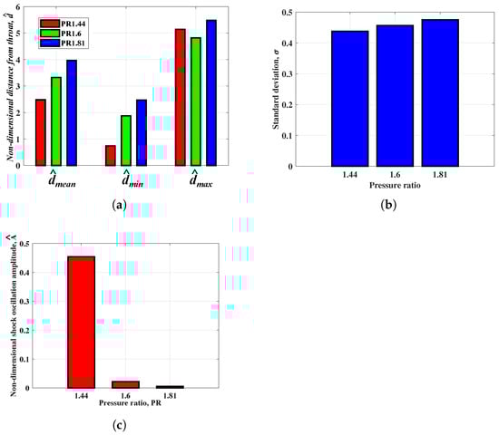
Figure 12.
Shock-wave position statistics: (a) Mean, maximum, and minimum positions of shock waves with respect to throat; (b) Standard deviation of the fluctuations related to shock-wave position data; (c) Amplitude of oscillations about the mean position of the shock wave.
3.5. Wavelet Transform of Pressure Data
The spectral analysis described heretofore provides a global overview of dominant pulsations within the flow. This section makes use of the aforementioned CWT (Section 2.6) methodology implemented on the pressure transducer data. Output from this transformation, that is, modulus of the Morlet transform, , has been presented as excerpts of the scalogram contour distribution plots in Figure 13. In the subfigures, the abscissa corresponds to time, the ordinate represents the frequency scale, and the color of the region presents the oscillation power of a particular frequency. Hence, blue corresponds to a lower , whereas yellow represents maximum . Notably, the first row (Figure 13a–c) corresponds to the scalogram plot upstream of the throat (P2AC), the second row (Figure 13d–f) represents the region near the throat (P1AC), and the third row images (Figure 13g–i) are related to the scalograms obtained using a pressure transducer placed downstream of the throat (P3AC). The value of PR increases from the left column to the right column. Contrary to FFT, scalogram excerpts exhibit intermittent modulation in amplitude, frequency, as well as temporal scales owing to the inherent shock-wave movement. Owing to the shock-wave motion unsteadiness, energy bursts related to the three dominant modulations do not emanate at all times, but intermittently, leading to commensurate time-evolving modulation of the pressure transducer data. Thus, CWT provides a comprehensive oversight of the shock-wave motion responsible for the low-frequency and large-time scale perturbations, and would further provide insights into the associated interactions.
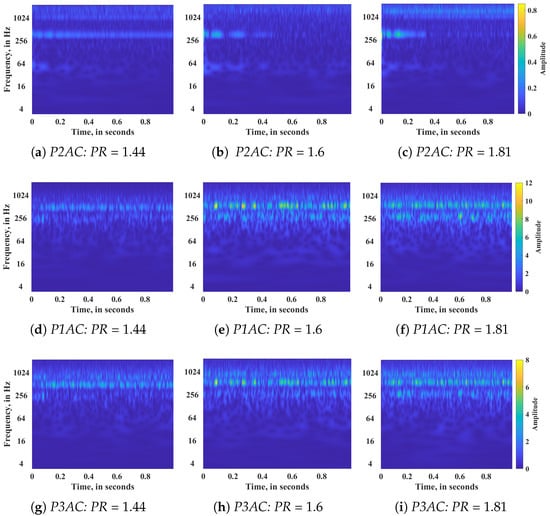
Figure 13.
Wavelet transform of time-wise pressure data obtained using high-frequency transducers.
Comprehensive differences between the upstream (P2AC) and downstream (P1AC–P3AC) spectral plots can be inferred from these plots. Pressure transducer, P2AC (Figure 13a–c), placed upstream of the throat, illustrates significant variation among the three PR cases. This port is associated with attached turbulent-boundary-layer flow. The presence of high-frequency, time-filling modulation beyond 1 kHz corroborates the presence of an attached turbulent boundary layer at this location. The presence of intermittency at this frequency modulation is proof of the intermittent character of incoming turbulent-boundary-layer flow. The bandwidth, magnitude, and consistency of this oscillation increase with PR, attributed to increased incoming turbulent-boundary-layer momentum. Apart from this high-frequency modulation, P2AC plots further illustrate the presence of modulation within the frequency band corresponding to FB2. The wavelet transform of P2AC for PR1.44 illustrates the presence of time-filling modulation around 500 Hz, which is close to the peak frequency of shock-wave pulsation, as determined in Figure 10 and Figure 11. Thus, this modulation is present across the entire duration for PR1.44, whereas it is limited to the first 0.4 s for PR1.6 and PR1.81. Notably, the intermittency is lower at this frequency compared to the intermittency observed earlier for high-frequency oscillations. Transonic flow through a nozzle has been associated with the presence of upstream acoustic feedback in earlier studies [66,67], with the upstream influence being higher for normal shocks. Thus, normal shock-wave oscillation that generates within the FB2 band for PR1.44, creates an acoustic feedback leading to time-filling oscillations of the wall upstream of the throat. However, as PR increases, the shock waves move downstream, separation and shear-layer intensity increase, and the shock wave becomes more oblique, leading to ameliorated upstream movement of the acoustic feedback. The initial energy bursts could be attributed to the presence of most upstream location interaction, leading to increased acoustic feedback (evident in Figure 13d). The synergized increment of power associated with these initial energy bursts at FB2, compared to the increased pulsating power of the spectrum plots at P1AC (compare Figure 13b with Figure 13e or Figure 13c with Figure 13f), further corroborates the increased impact of acoustic feedback from the moving shock waves. For all the cases, there is a time-filling low power modulation at around 50 Hz, which could be attributed to the incoming noise-related pressure fluctuations emanating from the roots blower motor.
Pressure data measured by P1AC will be a result of coupled interactions between the large-scale shock-wave motion, separation bubble dynamics, as well as high-frequency shear-layer eddies and flapping. Owing to these unsteadiness interactions, scalogram excerpts pertaining to P1AC (Figure 13d–f) display increased spectral power magnitude, a broadband frequency modulation, and variable intermittency across the various spectrum bands, attributed to spatial and temporal fluctuations associated with the shock waves. It can also be gleaned that the overall bandwidth of respective frequency modulations becomes wider, and their magnitude increases with PR increment (compare Figure 13d with Figure 13f). Thus, the enhanced incoming turbulence flow leads to broadband modulation of the pressure waves. The intermittent bursts associated with PR1.44 (Figure 13d) within the dominant FB2 band (around 500 Hz) exhibit a sparser and inconsistent modulation compared to the consistent and time-filling scalogram described earlier for P2AC (Figure 13a). The sparseness of frequency modulation increases from PR1.44 to PR1.6. Spectral peaks display increased variability for PR1.6, owing to the shock-wave motion being closer to this transducer. Thus, when the shock wave moves closer to the transducer, the amplitude increases. As it moves away, this amplitude decreases because of the increased influence of other interactions, which are associated with lower frequencies. Although the intermittency of FB2 is similar for PR1.81 (Figure 13f), the magnitude of this peak is reduced at this PR. This corroborates the reduced magnitude of the spectral peak within FB2 for PR1.81, as described earlier in Figure 10a. The downstream location of the shock wave with respect to the transducer for higher PR leads to a lowered amplitude of the associated oscillation.
Spectral plots pertaining to FFT in Figure 10 demonstrated the presence of an additional oscillatory phenomenon within FB1 (close to 250 Hz). The wavelet analysis in this section provides key insights into the time evolution of these oscillations. Its spectral power, frequency scale, as well as temporal scale, increased as PR increased. An interesting quasi-periodic trend pertaining to reciprocal exchange of spectral power between FB1 and FB2 can be observed at this location, especially for PR1.6 and PR1.81. The dominant shock motion pulse (FB2) exchanges energy with a lower-frequency oscillation (FB1), which could be associated with large-scale vortex shedding phenomena. Thus, as the separation bubble size increases, the spectral power of this instability increases, which ultimately dampens the shock motion, leading to reduced amplitude of the shock motion spectrum. This energy exchange phenomenon is significantly reduced for PR1.44 (Figure 13d), owing to the presence of normal shock dominance, leading to an assuaged impact of these vortices. It is also noteworthy that the temporal scale of FB1 and FB2 oscillations is commensurate with each other. For instance, in Figure 13e, the broad temporal scale of FB2 at 0.08 s and 0.28 s is followed by the broad temporal scale of FB1 fluctuations. On the other hand, the narrow energy bursts of FB2 between 0.5 s to 0.65 s are accompanied by intermittent narrow time FB1 peaks. This see-saw energy exchange phenomenon is observed for PR1.81 (Figure 13f). These results, along with the FFT plot of pressure data above, underline the presence of increased interdependence between the separation-zone breathing and the shock-wave motion, which corroborates the assertions drawn out by Pasquariello et al. [31]. It can also be noted that as PR increases, the overall magnitude of FB1 oscillations is higher, whereas it decreases for FB2 oscillations. Thus, as PR increases, the overall separation-bubble breathing enhances, leading to increased frequency of the associated global instability and higher spectral magnitude occurring over wider time-filling intervals. On the other hand, due to the further downstream location of shock waves for PR1.81, the overall impact of shock motion on P1AC is reduced. Increased PR leads to increased turbulence across the interaction due to vortex shedding within the shear layer. The impact of KH vortices, as depicted earlier in the Schlieren images, also increases as the separation shock impact enhances. This leads to the presence of intermittent modulations across higher frequencies extending beyond 1000 Hz (Figure 13d,e). This band residing within FB3 is associated with the shear-layer flapping, whose magnitude increases as PR increases. It can be discerned that the overall spread is wider for PR1.81 compared to PR1.6, indicating the broadband nature of turbulent fluctuations. The consistent intermittence of modulations pertaining to FB3 is further indicative of its relation to the turbulent interactions associated with SBLIs observed in this study.
As flow moves from P1AC to P3AC (Figure 13g–i), the magnitude pertaining to FB3 oscillations becomes wider in the frequency scale, whereas it retains the same bandwidth for the other two bands. This is expected, as the flow associated with P3AC will be linked with heightened turbulence-layer impact due to shear-layer thickening and vortex shedding. In fact, the presence of intermittent modulation around 960 Hz at this transducer for PR1.44 (Figure 13g), which was absent in the case of P1AC scalogram, as seen in Figure 13d, is associated with the shear layer at this location, leading to turbulent interactions. The magnitude of this high-frequency oscillation increases as PR increases because of the increased bulk momentum. Similar energy bursts as well as reciprocal exchange of spectral power between FB1 and FB2 oscillations pertaining to PR1.66 (Figure 13h) and PR1.81 (Figure 13i) are observed at this location. A subtle reduction in relative amplitude pertaining to FB1 is observed at this location compared to P1AC, because the downstream location leads to a mitigated impact of the separation-region instabilities. However, increasing the PR at this location (Figure 13i) leads to increased magnitude for FB1 oscillations because of the heightened flow separation characteristics of higher PR.
These plots eloquently illustrate the presence of varying intermittency, modulation in the temporal and frequency scales, as well as local high-energy pulses of varying temporal scales for different events [6]. Thus, the complex SBLI is a sum of numerous sparse events characterized by intermittency on the temporal scale, coupling between the different pulsations, as well as modulations associated with the shock motion and separation-layer breathing.
3.6. Spectral Analysis of Different Regions Within the Nozzle Flow at Different PR Values: Spatial FFT
After acquiring the temporal understanding related to these shock-wave oscillations on a global level, further insights regarding the underlying fluctuations within different sub-regions of SBLI are carried out in this section. This method involved carrying out an FFT analysis of time-resolved pixel intensities within specific regions called spatial FFT. For more details regarding this method, refer to the earlier section, Section 2.7. Figure 14 illustrates spectral energy plots derived by carrying out an ensemble-averaged FFT of grayscale values pertaining to different locations indicated earlier in Figure 5. As noted previously, ensemble averaging was carried out by making use of five different pixel locations within a specific region. The overall frequency resolution for this study was 5 Hz. Identifiers pertaining to different locations, that is, upstream Boundary Layer (BL), downstream BL, inviscid shock wave, reflected shock wave, and separation zone between the -foot oblique waves, are provided earlier in Figure 5 and presented again in the subfigure legends of Figure 14.

Figure 14.
Ensemble-averaged fast power spectral density of pixels related to different regions in the nozzle flow across different PR. The alphabets (a)–(e) are identifiers related to the specific region, which have been referenced in the associated explanation.
It can be seen from Figure 14a through Figure 14c that the pulsating power of the separation region is the highest, whereas it is similar for the shock wave and -foot region in all the cases. The spectral energy of these three regions is significantly higher compared to the upstream and downstream BL. This is expected as the unsteadiness associated with SBLIs is mainly linked with these interaction regions. Upstream and downstream regions are mostly the driving mechanism behind the low-frequency shock-wave oscillations, with the relative dominance based on the inherent separation intensity [13]. Notably, trends indicating similarity between the upstream–downstream BL signals, as well as between shock-wave- foot signals, with the latter presenting higher magnitude, were observed earlier in a 2021 experimental study by Ligrani et al. [14]. This provides credence to the validity of spectral trends captured in this analysis. In line with the earlier established stark difference in flow unsteadiness associated with PR1.44 compared to PR1.6 and PR1.81, spectral plots presented in this section also exhibit the same trend.
In the case of PR1.44 (Figure 14a), the downstream and upstream BL spectral energy distribution plots exhibit minimal divergence beyond 80 Hz, with the exception of a pronounced peak in the downstream spectrum near 460 Hz (similar to the FB1 peak observed earlier for shock-wave motion). While a corresponding peak is also evident in the upstream spectrum at this frequency, its amplitude is notably lower. Other than this localized deviation, the spectral characteristics across both regions present correspondence with each other. Given the increased effect of upstream BL (identified as (d)), on shock waves for lowered separation, spectral plots pertaining to the shock-wave region (a) display significant correspondence with the upstream spectral energy trend, especially at 460 Hz. The upstream data further displays trends similar to the shock wave up to 80 Hz, which is indicative of the low-frequency acoustic signals associated with pulsating separation bubble being present at both locations (which was indicated earlier in the FFT of shock-wave position data also). Moreover, both plots display the presence of spectral bursts around 460 Hz. Plots pertaining to downstream BL and separation zone display the dominant frequency peak at the same values, as the separation region associated with normal shock interaction flow is linked with pulsating separation layer rather than the shear-layer flapping effect. This results in uniform subsonic flow downstream of the shock wave, leading to similar spectral dynamics of the separation zone and the downstream boundary layer. The separation-zone plot demonstrates the presence of three peaks with frequency ranges analogous to the peaks observed earlier in the FFT plots of pressure data (Figure 10) as well as shock-wave position data (Figure 11). Thus, the separation region spectral energy distribution is directly linked with oscillations pertaining to shock-wave motion at this PR. Due to the normal shock-wave structure, the separation region fluctuates in sync with the shock-wave oscillations. The presence of similar spectral energy (both in magnitudes or overall pattern) across the shock wave and -foot region is attributed to the reduced influence of -foot waves in the case of PR1.44, leading to similar trends across the two regions. The increased difference between the shock wave (a) and the upstream BL (d) regions at higher frequencies indicates a lack of feedback between the separation region and the upstream BL at high frequencies.
As PR increases, PR1.6 and PR1.81 upstream BL plots in Figure 14b and Figure 14c, respectively, show increased magnitudes. This plot comes closer to the shock-wave- foot signals. In fact, the frequency-wise variation of upstream BL and shock waves displays similar trends, especially within the range of 200 Hz to 600 Hz. This similarity is maximum in the case of PR1.81. As PR increases, the separation zone and -foot magnitude also increase. This leads to increased feedback impact between the upstream and separation-zone regions, and hence the spectral plots display concurrence with regard to frequency-wise variations between the shock wave and upstream BL plots in this frequency range. The spectral energy for upstream BL in the case of PR1.44 was mainly limited to frequencies below 60 Hz, beyond which it dropped suddenly. However, as PR increased, the overall spectral energy was distributed across a wider spectrum, owing to increased momentum and hence turbulence. Owing to increased incoming turbulence, the spectral energy of the separation region also increased. This increased separation region intensity leads to increased vortex shedding, shear-layer flapping, as well as KH vortices. Thus, the overall spectrum for the separation region becomes more broadband for higher PR. In fact, the separation region plot in Figure 14c displays the maximum peak value at around 256 Hz, which was indicated earlier in the wavelet analysis (Figure 13) to be due to global instability associated with vortex shedding within the separation bubbles. Due to the increased PR, the impact of low-frequency noise (less than 60 Hz), separation region instabilities (200–500 Hz), as well as high-frequency vortical and turbulent eddies (more than 950 Hz) also increase. Increased spectral energy of upstream BL also contributes to the increased high-frequency oscillations in the separation region, an effect which increases as PR increases. The separation zone has dominant high-frequency peaks at PR1.44, whereas the low-medium frequency pulsations become more and more dominant at higher PR. Due to the combined impact of increased incoming turbulence and interaction turbulence, higher-frequency pulsations present a wider bandwidth for higher PR.
Broader differences can be observed between the shock waves and -foot at lower frequencies, which tail off at higher frequencies. Notably, the low-frequency signals are associated with large-scale oscillations. -foot signals are influenced by low-frequency oscillations pertaining to separation-bubble instabilities and shock-location unsteadiness, which lead to their elevated spectral power, amounting to increased disparity in relation to the shock-wave spectral plot. At higher frequencies, which are mostly affected by small-scale turbulence structures like KH vortices or shear-layer eddies, the frequency spectrum is more isotropic and affects the two regions uniformly. This accounts for their comparable spectral plots at high frequencies. The pulsating power of the -foot is closest to the separation zone plot at around 500 Hz for PR1.6 and PR1.81 cases. This would indicate that the pulsating power of the underlying separation bubble, at different PR, would directly impact the spectrum of separation shocks [32]. Spectra pertaining to shock waves and upstream BL indicate concurrent frequency-wise variations, indicating comparable oscillation dynamics. This similarity further confirms the presence of increased feedback between the upstream BL and shock-wave regions for higher PR.
Downstream BL plots display similar trends across the three PR cases. However, the coupling of different interactions results in different peaks, as well as variations in the high-frequency spectrum. For PR1.44 and PR1.6, downstream BL displays the presence of peaks placed closer to each other. However, as PR increases to 1.81 (Figure 14c), these peaks become more widespread while increasing the magnitude for pulsations within the high-frequency FB3 spectrum. At PR1.44, this peak occurs in sync with the separation region peak due to flow being associated with subsonic flow, leading to propagation of information from the normal shock wave to the downstream BL, and hence similar pulsation dynamics. On the other hand, for PR1.6 and PR1.81, this region became affected by the separation-layer breathing (near 220 Hz) or shear-layer unsteadiness (around 500 Hz), as well as shear-layer entrainment [23]. The spectral power of these large-scale instability interactions is higher compared to the underlying higher-frequency small-scale pulsations embedded within the downstream BL. Due to the combined effect of these factors, the downstream BL displays a wider range of frequency-wise perturbations for higher PR. It is also noteworthy that the peaks related to downstream BL at PR1.44 were linked with oscillations pertaining to shock position (around 500 Hz). However, as PR increased, this peak magnitude was reduced significantly due to increased coupling of other flow interactions. Moreover, the presence of an increased separation region mixing, the magnitude of lower-frequency pulsations also starts increasing. In fact, the downstream BL plot pertaining to PR1.81 in Figure 14c displayed the presence of an additional peak at a much lower frequency (170 Hz), which could be attributed to the shear layer-driven breathing of the separation zone, leading to lowered frequency [23]. The plots pertaining to the separation zone further exhibit the presence of modulations below 100 Hz for higher PR, which could be related to the separation-region breathing effect. This shall be corroborated further using coherence analysis in a later section.
Overall, the spatial FFT analysis across PR1.44, PR1.6, and PR1.81 presented in this section reveals a clear shift from high-frequency-dominated separation dynamics at lower PR to increased low-frequency pulsations and broader spectral bandwidth at higher PR. This is driven by stronger upstream turbulence and enhanced separation-bubble breathing. With increasing PR, upstream boundary layer, shock wave, -foot, and separation-zone spectra become more correlated, while downstream-boundary-layer peaks diversify due to evolving influences from shear-layer unsteadiness, entrainment, and large-scale instability structures. These trends emphasize the strengthening of the feedback mechanism and turbulence coupling within the studied SBLI as PR rises.
3.7. Coherence and Time-Lag Analysis Between Different Regions Within the Nozzle for Different PR
The current section discusses frequency-wise correlation between different interaction regions using magnitude-squared coherence and time-lag quantities. These results would examine the correlation between various frequency-specific events discussed during the previous sections. An earlier study carried out by Ligrani et al. [14] assessed correlation variation within different regions to understand the unsteadiness related to normal shock waves. Considering the distinct flow characteristics for oblique waves compared to normal shock waves, as elaborated by Dussauge et al. [12], this section aims to expand the understanding related to the correlation between different regions for SBLIs characterized by varying PR conditions that would shed further insights into the underlying flow physics.
Identifiers related to coherence between the different regions measured in this section are tabulated in Table 8. Figure 15, Figure 16, Figure 17, Figure 18, Figure 19, Figure 20, Figure 21 and Figure 22 compare the coherence distribution pertaining to these regions, which are followed by Figure 23, Figure 24 and Figure 25 pertaining to the time-lag of frequency-specific events across different regions.
Table 8.
Identifiers for coherence evaluated across different regions.

Figure 15.
Ensemble-averaged comparison of magnitude-squared coherence between shock wave and downstream boundary layer pixels at different pressure ratios.
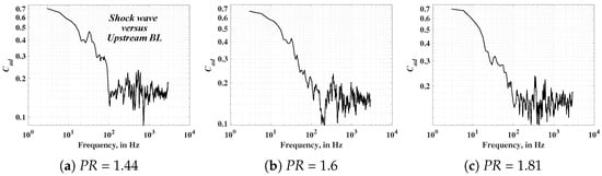
Figure 16.
Ensemble-averaged comparison of magnitude-squared coherence between shock wave and upstream boundary layer pixels at different pressure ratios.
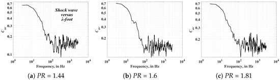
Figure 17.
Ensemble-averaged comparison of magnitude-squared coherence between shock wave and -foot pixels at different pressure ratios.

Figure 18.
Ensemble-averaged comparison of magnitude-squared coherence between the shock wave and pixels related to the separated region behind the shock wave at different pressure ratios.

Figure 19.
Ensemble-averaged comparison of magnitude-squared coherence between the separation zone and pixels related to the downstream pixel at different pressure ratios.
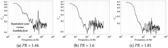
Figure 20.
Ensemble-averaged comparison of magnitude-squared coherence between separation zone and pixels related to the lambda-foot signal at different pressure ratios.
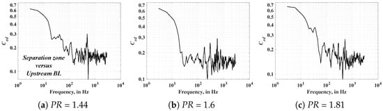
Figure 21.
Ensemble-averaged comparison of magnitude-squared coherence between the separation zone and pixels related to the upstream pixel at different pressure ratios.

Figure 22.
Ensemble-averaged comparison of magnitude-squared coherence between upstream and downstream boundary layer pixels at different pressure ratios.
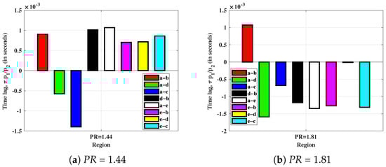
Figure 23.
Time lags between different regions for oscillations between 100 and 280 Hz.
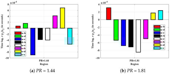
Figure 24.
Time lags between different regions for oscillations between 500 and 600 Hz.

Figure 25.
Time lags between different regions for oscillations between 800 and 900 Hz.
Figure 16 compares the coherence between the shock wave and the downstream BL pixels (). At PR1.44, Figure 15a indicates the presence of increased coherence () of the order of at 500 Hz, which was indicated earlier to be the primary shock-wave oscillation frequency. The associated value presented in Figure 24a indicates a positive time lag, which conveys the convective attribute of the associated event. Thus, the shock-wave oscillations are transmitted directly to the downstream BL at PR1.44, leading to the concurrent FFT spectrum for downstream and shock-wave signal indicated above in Figure 14a. In fact, the presence of coherence ranging beyond , as well as positive for all frequencies (Figure 23a, Figure 24a and Figure 25a), further backs up the direct correlation of shock-wave signal with downstream BL fluctuations at PR1.44. However, as PR increases, this concurrence is significantly lowered, leading to mitigated coherence between the shock wave and downstream BL signals beyond 100 Hz. In fact, the coherence becomes more widespread, amounting to increased coherence values at higher frequencies. Thus, the downstream flow is affected by small-scale, high-frequency events like KH vortices. The presence of positive at PR1.81, indicated in Figure 24b and Figure 25b pertaining to a-b interaction, further confirms the convective attribute of these oscillations at high frequency and higher PR. A downstream BL event that affects the shock-wave oscillation is called the shear-layer entrainment effect, which leads to recharge of the shear-layer instabilities in the downstream direction, leading to flapping of the shear layer. The presence of increased coherence at a frequency close to 180 Hz in Figure 15c further supports that this phenomenon is related to downstream-boundary-layer fluctuations. Explanation regarding the coherence peaks at frequencies below 100 Hz and above 980 has been included later.
Significant coherence between shock wave and upstream BL events () for PR1.44 in Figure 16a is indicated by the presence of high () at 290 Hz and 530 Hz. Time lag () estimates display a negative value for events pertaining to 100 Hz to 280 Hz (Figure 23a), whereas at 500 Hz, this value becomes positive, as seen in Figure 24a. The low-frequency oscillations attributed to “breathing” follow a convective upstream BL → downstream BL path, whereas the subsonic flow downstream leads to high-frequency oscillations becoming easily transmitted to the upstream BL from the shock wave. This was again indicated in the scalogram plot pertaining to wavelet analysis of pressure data, wherein the plot pertaining to PR1.44 displayed the presence of time-filling energy bursts related to 500 Hz (Figure 13a). At higher PR values, the effect of oblique shock waves and shear layer increases. Thus, the increased flow-separation intensity leads to heightened convective vortex shedding in the downstream direction. The presence of negative (Figure 23b and Figure 24b) further emphasizes the presence of convective features related to these oscillations (FB1 and FB2).
The coherence between shock wave and -foot signals designated as in Figure 17 is strongly related to the coupling of motions related to these complex flow attributes. At low PR (Figure 17a), due to the dominance of normal shocks, motions associated with them are tightly coupled, leading to increased influence of the large-scale (low-frequency) oscillations associated with shock-wave motion. This is indicated by the delayed shortfall of coherence, which occurs at lower frequencies for higher PR. This leads to increased mean coherence for PR1.44 compared to PR1.6 and PR1.81. At higher PR, the coherence is influenced by the oscillations associated with high-frequency, low-scale oscillations in the separation region. This amounts to increased impact of the high-frequency components, leading to increased fluctuations of coherence at higher frequencies. Associated exhibits a negative value for all the frequency ranges apart from FB3 pulsations in both the PR cases. The presence of negative for the low-medium frequency bands (Figure 23a and Figure 24b) indicates the relevance of shock-wave oscillations on the oscillations of -shock oscillations, which are associated with separation region oscillations, especially for higher . The value of within FB3 (800–900 Hz), as seen in Figure 25a,b, presents positive values for both cases. Thus, the high-frequency oscillations associated with turbulence bursts follow a convective mechanism from the shock towards the -foot waves.
Figure 18, Figure 19, Figure 20 and Figure 21 discuss the coherence between the separation zone (e) and the other regions (a), b, c and d). At (Figure 18a), exhibits a significant coherence of at around 500 Hz. It also has significant peaks at the frequencies close to the dominant peaks of shock-wave oscillations detected earlier, that is, within FB1 and FB3 bands, which indicates a strong correlation between shock-wave and separation-zone oscillations. At higher , the separation zone becomes more complex, and hence the peaks become less prominent due to increased intermixing (Figure 18b,c) and the effect of global instabilities. Despite the lowered peak values, the overall fluctuations indicate a pattern similar to FFT plots mentioned earlier for shock-wave position data, with maximum coherence at FB2 (≈24%), and subdued peaks (≈18–20%) for oscillations lying within FB1 and FB3. The presence of negative in Figure 23b, Figure 24b and Figure 25b at all frequencies for both cases (except PR1.44: 100–200 Hz) indicates a prominent feedback phenomenon between the separation zone and to shock wave governing the primary oscillation peaks. The presence of positive at FB1, for PR1.44, is related to the presence of increased normal shock impact, leading to mitigation of separation breathing effect at this PR, with the flow being mainly dominated by pulsating global instabilities related to large-scale oscillations.
Owing to the increased influence of separation-zone unsteadiness on the overall shock-structure instabilities, further assessment regarding coherence and time-lag evaluations pertaining to oscillations in the separation zone (e) with respect to other regions that—namely, downstream BL (b), -foot (c) and upstream BL (d)—is discussed in Figure 19, Figure 20 and Figure 21, respectively. Coherence presents the maximum coherence (>70%) within FB2, followed by subdued local maximum coherence peaks at FB1 and FB3 bands of oscillations. Similar heightened coherence was found for the shock wave versus the downstream BL earlier in Figure 15. The presence of positive (Figure 23a, Figure 24a and Figure 25a) indicates that these events occur at the separation zone and then are transmitted to the downstream location without much deterioration. Thus, owing to the normal-shock structure, tight coupling between the shock wave, downstream BL, and separation zone exists; hence, the underlying unsteadiness of the structure is defined by the downstream motion of the shock-wave instability. Global instability associated with coherent structure within the separation region is the driving mechanism related to these shock-wave oscillations at PR1.44. As PR increases (Figure 19b,c), the value of frequency associated with maximum increases. However, the amplitude of this peak reduces as the overall unsteadiness becomes more widespread and is influenced by high-frequency oscillations related to shear-layer turbulence, as well as KH vortices. Interestingly, the plots also present the local coherence peaks close to 165 Hz. This frequency pulse was indicated earlier for the downstream BL in the spatial FFT plot of Figure 14, associated with downstream BL flapping. Thus, contrary to the PR1.44 case, flow unsteadiness at PR1.6 and PR1.81 is influenced by pulsation of the separation region, shear-layer fluctuations, as well as global instabilities. The presence of negative in Figure 23b, Figure 24b and Figure 25b is indicative of the increased feedback from the downstream shear-layer boundary layer for higher PR.
The presence of alignment between the frequency peaks of FFT (Figure 11) plot pertaining to shock-wave position data and the coherence estimation, as shown in Figure 19a, provides further credence to the fact that coherence estimates in this section are forced by the flow physics rather than visual artifacts.
Although the peak coherence between the separation zone and -foot events () at PR1.44 is reduced to , the separation zone exhibits increased correlation with respect to -foot events analogous to shock waves presented earlier in Figure 18. This validates the increased interaction dynamics between events pertaining to -foot and separation-zone oscillations. In line with described above, also presents an increase in the value of frequency, where coherence is maximum as PR increases (Figure 20b,c). It can also be seen that the overall plot demonstrates the presence of higher up to an extended range of oscillations beyond 100 Hz for PR1.44, which indicates the presence of increased influence of low-frequency separation bubble pulsation on the -foot structure. The value of becomes more widespread as the increases, which is coincident with the trends observed earlier for . Hence, the interaction dynamics between the shock wave and the -foot are influenced by increased shear-layer flapping, as well as global instabilities leading to higher-frequency oscillations. The presence of negative presented in the time-lag plots further confirms that these oscillations, especially the high-frequency oscillations, originate at the -foot and then reach the separation zone.
Figure 21 and Figure 22 compare the magnitude-squared coherence of the separation zone and downstream BL fluctuations with upstream BL, that is and , respectively. In the case of , the plots demonstrate the presence of peak coherence values () within FB2, with the frequency value increasing from PR.1.44 to PR1.6, while retaining similar values between PR1.6 and PR1.81. At lower PR values, the overall is mainly influenced by the global instability of the shock-wave oscillations within FB2, whereas at higher (Figure 21b,c), there is increased coherence peaks at values lower than the prominent peak due to increased shock pulsation effect corresponding to lower frequencies. The presence of positive for all the cases suggests the presence of upstream movement of these oscillations from the separation zone. Increased leads to increased spectral energy of the incoming flow, leading to downstream placement of shock waves; hence, the effect of shear-layer oscillations, vortex shedding, flapping effect, and pulsation bubble increases.
It has been postulated by Pirozzoli et al., 2010 [65] that the upstream BL acts as a forcing mechanism to sustain the low-frequency breathing of the separation region pertaining to SBLIs. Figure 22a elaborates the presence of increased of at around 500 Hz (main shock-oscillation frequency). Thus, the shock wave’s large-scale oscillation impacts the upstream and downstream locations similarly at this frequency for PR1.44. The normal shock-wave structure enables convective and feedback flow of disturbances from the breathing separation bubble in both directions. The presence of negative further emphasizes the seeding of this oscillation in the separation zone. As the PR increases, the effect of other oscillations also increases, leading to a more uniform distribution beyond 100 Hz (Figure 22b,c). This negative is presented for almost all the cases, further emphasizing its source of origin being downstream of the upstream BL. A distinct peak close to 150 Hz can be observed at PR1.81, which is concurrent with the peak observed earlier in Figure 14c, related to the separation-layer breathing effect, which is transmitted to both directions, leading to this peak. The presence of positive at this frequency for PR1.44 (Figure 22a) indicates that this low-frequency oscillation acts as a driving force for this breathing at such a lower PR, whereas at higher PR, the upstream BL is mainly influenced by the feedback phenomena, which is higher because of increased global instability of the separation bubble.
Coherence associated with oscillations below 100 Hz presented an increase in magnitude-squared coherence across different regions at lower PR. This indicates a stronger upstream influence of pulsating bubbles on the acoustic feedback, leading to increased impact of these oscillations originating within the interaction. As increases, the impact of this acoustic feedback reduces and the influence of high-frequency oscillations increases. Consequently, the drop in coherence is delayed with higher PR for much of the cases. These trends are applicable across all the coherence plots. However, in Figure 22c exhibits the presence of increased coherence values (more than ) for higher with a negative (Figure 25b). This occurs because the increased amounts to increased low-frequency oscillations in both directions owing to increased separation bubble pulsation. These pulsations lead to comparable coherence in both directions, leading to increased low-frequency coherence for downstream BL versus upstream BL at higher PR.
3.8. Numerical Analysis of SBLIs at Different Pressure Ratios
To complement the experimental visualizations of flow structure, numerical Schlieren reconstructions were generated from the simulated flow fields for each pressure ratio. These images, shown in Figure 26, qualitatively capture the shock-wave structure and separation patterns within the nozzle. The selected time frames correspond to the farthest downstream appearance of the shock system, allowing direct comparison with the experimental frames presented earlier.

Figure 26.
Computationally reconstructed Schlieren images for three pressure ratios: PR = 1.44 (top), PR = 1.6 (middle), and PR = 1.81 (bottom). The frames correspond to the approximate maximum extent of the -foot formation in each case. The images show density-gradient magnitude, highlighting shock structures and flow-separation regions. Increasing PR leads to a downstream shift and sharpening of the shock system, reflecting the growth of the separation region and a more coherent interaction pattern.
Similarly to the experimental observations, the numerical results reveal a progressively downstream movement of the shock system with increasing pressure ratio. For PR1.44, the simulations predict a normal-scale -foot, in contrast to the nearly flat, small-scale structure observed experimentally. For PR1.6 and PR1.81, the -foot becomes larger, corresponding to a lower Mach disc at the same stage of motion, consistent with the experimental trend. Across all PRs, the -feet appear closer to the throat compared to the experiment, though the relative progression with increasing PR is reproduced. Other key features—including shock curvature, wave interactions, and the extent of separation—are also well captured, reinforcing the fidelity of the simulation approach in representing the dominant characteristics of the SBLI.
3.9. Spectral Analysis of Numerical Pressure Data
To investigate the unsteady behavior of shock-induced pressure fluctuations, FFT was applied to the numerically derived time-resolved static pressure signals obtained from four monitoring locations: P20, P26 (corresponding to the experimental transducer P1AC), P26y (directly beneath P26 on the lower wall), and P3AC, a perpendicular plane near the end of the diverging section that monitors the area-weighted average of static pressure. P20 was selected because, for lower PRs (particularly PR1.44), the shock does not extend far enough downstream to influence P26, ensuring that the signal remained within the effective shock oscillation zone. Additionally, P20 consistently exhibited stronger oscillation amplitudes, making it well-suited for visualizing the frequency characteristics of the flow.
Figure 27 presents the amplitude spectra for PR1.44, PR1.6, and PR1.81. Part (a) shows P20, P26y, and P1AC, which exhibit very similar frequency distributions. P26y reproduces nearly identical spectra to P1AC despite lying beneath the shear layer, confirming the presence of the same dominant frequencies on both the upper and lower sides of the asymmetric -wave structure. Part (b) presents the spectra from the P3AC plane, which closely resemble those in part (a), consistent with the experimental results in Figure 10. For PR1.44, three distinct frequency regions are observed between 250 and 900 Hz, with peaks at 265 Hz, 510 Hz, and 800 Hz. For PR1.6, the frequencies shift upward while maintaining three regions: peaks near 280 Hz, two peaks around 545 Hz, and multiple peaks near 905 Hz. For PR1.81, the three regions show a single peak at 305 Hz, another at 660 Hz, and multiple peaks around 970 Hz. Notably, for the first frequency region across all PR cases, the numerical results exhibit an increasing trend in peak frequency, whereas the experimental observations show a slight decrease in frequency for PR1.6.
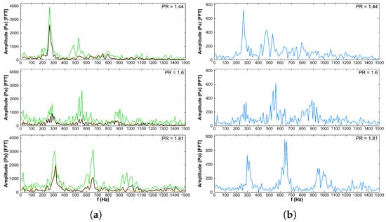
Figure 27.
Amplitude spectra obtained from FFT of static pressure signals at (a) P20 (green line), P26y (orange line), and P1AC (black line), and (b) the P3AC plane, for three pressure ratios: PR1.44, PR1.6, and PR1.81. P20 was chosen to ensure the signal remained within the shock-oscillation zone across all PR cases and consistently exhibits higher spectral amplitudes. The similarity of the spectra across monitoring locations and the upward shift in dominant frequencies and amplitudes with increasing PR closely reflect the experimental observations.
The consistent trends of increasing dominant frequency and amplitude with rising PR highlight the intensification of shock motion and its interaction with the boundary layer, producing broader and more energetic spectra. The agreement of numerical and experimental results in both frequency and amplitude confirms that the simulations effectively capture the key unsteady flow features and coherent oscillations throughout the interaction region.
3.10. Numerical Shock-Wave Dynamics Analysis
To complement the spectral analysis, the temporal evolution of the shock-wave position was tracked in the numerical simulations for all three pressure ratios. The axial position of the shock front was extracted in time and analyzed to identify its minimum and maximum extent relative to the throat. The results, presented in Figure 28, indicate that the range of shock motion increases with rising PR: for PR1.44, the shock oscillates between m and m downstream of the throat; for PR1.6, the range extends from m to m; and for PR1.81, from m to m. The negative minimum value for PR1.44 indicates that the shock occasionally moves slightly upstream of the throat, likely due to weak separation and local flow instabilities at lower pressure ratios. Although these upstream excursions are not observed in the experiments, where all positions remain downstream of the throat, the overall trend of increasing downstream shift with PR is captured.

Figure 28.
Shock -wave position over time (left) and corresponding FFT of the axial shock coordinate (right) for three pressure ratios (PR = 1.44, 1.6, and 1.81). The shock location is determined from the maximum Schlieren intensity along a line parallel to the channel axis, with 0 corresponding to the throat. The left panel shows the temporal evolution of the shock, where an increasing pressure ratio leads to a downstream shift and smaller oscillation amplitude, indicating a reduced range of axial motion. The right panel presents the FFT of the shock position, highlighting distinct frequency regions for each pressure ratio, similar to the static pressure FFT results but with clearer separation of dominant frequency bands.
Further insight into the unsteady behavior of the shock was obtained by analyzing its axial position in the frequency domain using FFT. The amplitude spectra of the shock position over time are shown in the right panel of Figure 28. Similarly to the FFT of static pressure signals, the shock position spectra exhibit multiple distinct frequency regions for each pressure ratio, reflecting the dominant oscillatory modes of the shock system.
Statistical parameters of the numerically derived shock motion were extracted from the time-resolved position data. Table 9 presents the mean position, minimum, and maximum positions, standard deviation, and oscillation amplitude of the shock wave, normalized by the throat height. The mean shock position increases monotonically with PR, consistent with the experimentally observed downstream migration. However, unlike the experimental data, where the standard deviation increases with PR, the numerical results show a decreasing trend: drops from 0.46 at PR to 0.24 at PR . This discrepancy may result from inherent smoothing and numerical dissipation in the URANS simulations, which dampen short-scale fluctuations that are present in experiments. Similarly, the oscillation amplitude decreases with increasing PR, from 1.85 to 1.05, reflecting the reduced range of large-scale shock excursions both in the experiment and in the numerical models.
Table 9.
Statistical metrics of shock-wave position obtained from numerical simulation, normalized to throat diameter.
The negative minimum shock position observed for PR1.44 highlights the sensitivity of the shock to upstream flow perturbations under weak separation conditions. In contrast, higher PR cases exhibit strictly positive minimum positions, indicating that the shock remains fully downstream of the throat. Overall, the numerical results reproduce the main characteristics of the shock motion, capturing the downstream shift in the mean position and the general reduction in oscillation amplitude with increasing pressure ratio, while differences in standard deviation trends compared to experimental observations are likely due to the smoothing effects of the numerical scheme. These simulations will act as a benchmark for future detailed numerical evaluations pertaining to SBLIs in the context of over-expanded flow through a typical convergent–divergent nozzle.
It is important to emphasize that the physical mechanisms underlying the low-frequency oscillations remain not fully understood. In particular, scaling laws for their frequency have yet to be firmly established. Therefore, direct comparisons with the experimental results currently lack a solid theoretical foundation. The adjustable experimental rig utilized in this paper holds significant potential for advancing this understanding and establishing such scaling laws through systematic studies. Hence, the numerical study carried out at this stage presented a qualitative comparison only. Owing to the preliminary stage of numerical evaluations, this paper presented results obtained using a moderate computational framework: URANS, avoiding the need for an extremely fine mesh or extensive CPU time. The primary aim of these simulations was to determine whether such a simplified model could qualitatively reproduce the observed low-frequency shock-wave oscillations and capture the general structure of the shock and boundary-layer separation. Encouragingly, the results show a strong overall agreement with the experimental data.
It is envisaged that as the experimental campaign progresses and more parametric data become available, the numerical modeling approach will also be refined using higher-fidelity techniques such as Detached Eddy Simulation (DES), Large Eddy Simulation (LES), and Scale-Adaptive Simulation (SAS) techniques, which will result in a more detailed quantitative comparison between simulations and experimental results. Such analysis in the future will provide valuable insights not only into the flow physics but also into the performance and limitations of the numerical models.
4. Conclusions
The current work was initiated by presenting a detailed experimental evaluation of unsteadiness related to streamwise oscillations of shock-wave–boundary-layer interactions (SBLIs) within an over-expanded De Laval nozzle, operated across different nozzle pressure ratios (PR) conditions. The experimental results were analyzed through the implementation of several spectral techniques, as well as correlation analysis techniques, with the aim of discerning dynamics related to the emanating shock-wave and boundary-layer flow structures and the interactions thereof. It is envisaged that fundamental understanding acquired through these studies could prove helpful in selecting the most appropriate nozzle geometry for improved performance while enhancing fundamental understanding related to the current state-of-the-art in SBLIs across transonic flow.
The experimental investigations used in this study were carried out within the air-vacuum experimental setup installed at the Department of Power Engineering and Turbomachinery, Silesian University of Technology, located in Gliwice, Poland. The required transonic flow (Mach number 1.2 to 1.3) conditions pertaining to variable PR were achieved by adjusting the flow rate through the usage of a series of control valves and a roots blower. The high-speed experimental setup made use of thirty digital and three high-frequency pressure transducers placed at appropriate locations to analyze flow unsteadiness across the nozzle. This measurement system was accompanied by a basic knife-edge Schlieren visualization technique that captured high-definition time-varying, shock-wave flow features within the test section. The two synchronized measurement systems were employed to capture accurate density fluctuations, as well as pressure oscillations at critical locations within the flow: that is, the inlet, throat, and outlet of the test section. A separate image processing technique using the Canny algorithm was implemented to track the shock-wave position and carry out further image spectral analysis. These high-contrast images and pressure readings acquired at a rate of 6000 samples per second were further analyzed using Fast Fourier Transform (FFT), Continuous Wavelet Transform (CWT) and coherent analysis techniques to enhance understanding related to interaction dynamics between the upstream boundary layer, inviscid Mach disk, oblique reflected shock wave, breathing separation region, and the downstream boundary layer.
The preliminary aerodynamic assessment made use of the isentropic relations applied to the pressure data to ascertain the Mach number distribution within the nozzle at different PRs. The trends indicated the presence of a typical nozzle expansion sequence, initiated by expansion within the converging section, sudden shock compression downstream of the throat, and terminating with pressure recovery. PR increment led to increased Mach number, at the expense of increased adverse pressure gradient, as well as a prominent asymmetric -shock structure, occurring at a later position downstream of the throat. Preliminary visualization of the flow structure at different PRs illustrated the increased influence of PR variation on the SBLI flow structure and interactions therein. Elevated PR led to increased complexity of the SBLI structure owing to a prominent -foot structure, increased density fluctuations downstream of the shock, increased flow mixing attributed to Kelvin–Helmholtz (KH) vortices, as well as increased shear-layer unsteadiness. Large-scale stream-wise oscillations were discovered for all the cases. Reconciliation of the reasons responsible for these oscillations was established using a detailed spectral analysis thereafter.
In the first stage of this analysis, the classical Fast Fourier Transform (FFT) technique was applied to the time-resolved pressure and shock-wave position data. These investigations emphasized the presence of three distinct spectral peaks between 240 and 990 Hz associated with the overall flow unsteadiness. The frequency value of these primary peaks was commensurate with the PR value, with a higher PR leading to a higher-frequency value and associated magnitudes. The first two peaks were indicated to be related to the large-scale shock-wave oscillations, whereas the higher-frequency peaks were associated with the underlying shear-layer instabilities and turbulence, similar to inferences drawn earlier by Pirozolli et al. [65]. The plots also demonstrated the presence of increased correlation between the pressure data at the throat and the diverging section, which is indicative of dependence of the downstream fluctuations on the throat location, which would ultimately affect the overall performance of a nozzle. The FFT of the shock position data also presented the existence of three prominent oscillatory events analogous to the pressure data FFT. The results further indicated the presence of heightened variations between and compared to subdued variations between and variants. This disparity was associated with the significant variation in flow structure. The low PR variant that is was linked with normal shock structure, whereas the higher PR variants were associated with increased -foot influences, leading to increased flow mixing, turbulent interactions, and high-frequency oscillations. The low flow was linked with increased upstream turbulence effects, leading to a number of small-scale frequency peaks below 100 Hz that were absent for higher PR variants. Furthermore, increased bulk momentum of the flow linked with higher led to increased feedback within the SBLIs, leading to a further downstream location of the mean wave position, followed by a lower amplitude of shock-wave oscillations about the mean shock-wave position. The plots also demonstrated that as the effect of -foot increases, small-scale oscillations associated with broadband frequency pulsations become more prominent, and are showcased as increased high-frequency spectrum magnitudes across a wider bandwidth of oscillations.
Motivated by the work of Bernardini [6], comprehensions regarding the temporal evolution of global kurtosis of pressure data at different values were carried out through the implementation of Morlet function-based CWT. The associated scalogram excerpts depicted the presence of varying intermittency, modulation in the frequency and temporal scales, as well as local high-energy pulses of varying temporal scales. The plots further concluded that the overall SBLI is a result of numerous sparse events characterized by intermittency in the temporal scale, coupling between the different pulsations, as well as modulations associated with the shock motion and separation-layer breathing. The upstream port (P2AC) exhibited increased impact of the intermittent high frequency (more than 1 kHz) attached turbulent boundary layer, followed by increased acoustic feedback upstream at frequencies closer to the peak oscillatory frequencies of shock waves (around 500 Hz). The high-frequency intermittent energy bursts were more time-filling, whereas the acoustic feedback was lowered across higher PR experiments. Increased spectral magnitude along with heightened bandwidth of modulations within different frequency bands were observed at the transducer placed close to the throat owing to increased influence of the shock-wave motion, separation bubble dynamics, and shear-layer instabilities. CWT further presented the variation of sparseness of intermittent frequency modulations, amplitude of oscillations across the different PR conditions. The three cases further presented quasi-periodic trends associated with energy pulsation between the frequency band one: FB1 (around 250 Hz) and FB2 (around 500 Hz), amounting to energy exchange between the pulsating separation bubble and shock-wave oscillation, with the effect being more significant for higher PR. Increased PR also led to increased impact of high-frequency pulsations like shear-layer flapping, KH vortices, leading to more pronounced modulations at frequencies beyond 1000 Hz. The transducer P3AC presented similar trends to those of P1AC. However, the plots further displayed increased high-frequency magnitudes owing to shear-layer thickening and vortex shedding. Increased PR at this location also led to increased magnitude of FB1 oscillations. Higher PR leads to increased separation-bubble breathing, leading to increased frequency of the associated global instability and higher spectral magnitude occurring over wider temporal scales.
Further assertions regarding the underlying unsteadiness were carried out by implementing a detailed spatial FFT investigation that involved carrying out an FFT of time-resolved pixel intensity signals pertaining to different regions within the context of SBLI, namely the upstream boundary layer (upstream BL), downstream BL, normal shock wave, downstream -foot, and separation-zone pixels. At PR1.44, separation -one pixels demonstrated the presence of similar frequency peaks that were detected by the earlier FFT plots, indicating the convection of shock motion oscillations in the separation zone. At this PR, the downstream BL was linked with increased convective motion of shock motion, providing a convective peak at FB2, whereas upstream and shock wave displayed increased correspondence, especially at FB2. Owing to the increased normal shock effect and reduced -foot flow characteristics at this PR, similar frequency bursts were presented by downstream BL and separation-zone plots. At increased PR, the spatial FFT plots demonstrated increased feedback between the separation-zone and upstream BL spectra within 200 to 600 Hz, leading to increased spectral energy compared to PR1.44. The spectral energy of the separation zone increased due to heightened incoming flow turbulence. However, this energy was distributed across a wider bandwidth, with the overall trend exhibiting the influence of the vortex shedding on the overall separation breathing. The elevated PR led to the increased impact of low-frequency noise (less than 60 Hz), separation region instabilities (200 Hz to 500 Hz), as well as high-frequency turbulent fluctuations spread across a wider bandwidth. Increased interactions between the separation zone and -foot signals at low-medium frequency energy spectra were observed for higher PR. The downstream BL further presented increased spectral energy across a wider bandwidth at higher frequencies, with the overall trend transitioning from increased influence of shock-wave oscillations at lower PR to increased influence of low-frequency separation-breathing zone at higher PR. The spatial FFT trends highlighted the increased influence of feedback mechanisms and coupled turbulence interactions within the studied SBLI as PR rose.
At PR1.44, strong coherence was observed between shock-wave oscillations and downstream BL, upstream BL, -foot, and separation zone, with the dominant 500 Hz mode transmitted following a convective path across the regions. The separation zone showed particularly high coherence with downstream BL (>70%) and significant interaction with -foot and shock motion, confirming its central role in driving unsteadiness. Time-lag analysis indicates both downstream convection of shock-induced oscillations and upstream feedback from the separation zone, with low-frequency breathing modes propagating in upstream and downstream directions. As PR increased, overall coherence was mitigated and shifted towards higher frequencies, with flow unsteadiness increasingly governed by shear-layer instabilities, KH vortices, and global separation dynamics. Coherence peaks were more wide-band, separation–shock coupling was reduced, and -foot and boundary layer interactions became dominated by small-scale, high-frequency oscillations. Overall, the coherence analysis highlighted that at lower PR, shock-separation dynamics were tightly coupled through a dominant 500 Hz oscillation, whereas at higher PR, the flow transitioned to a regime where global instabilities, vortex shedding, and high-frequency shear-layer effects governed the interaction, reducing direct coupling and redistributing energy across a wider spectral range.
Complementing the experimental findings, numerical simulations using transient 3D RANS provided further insight into the unsteady shock motion and -foot dynamics. Time-resolved shock position data extracted from the simulations revealed a downstream shift in the mean shock location with increasing PR, along with a reduction in oscillation amplitude, consistent with the experimental trend. FFT analysis of the shock axial position confirmed the presence of multiple frequency regions analogous to those observed in the static pressure signal spectra, demonstrating that coherent oscillations persist across the shock and separation regions. Notably, the first frequency region exhibited an increasing trend in the numerical results with PR, whereas the experiments showed a slight decrease at PR1.6, highlighting the subtle influence of upstream boundary layer fluctuations and numerical smoothing inherent to URANS approaches. Further comparison of spatial and temporal spectra between the experiments and simulations indicates that the dominant frequencies associated with large-scale shock oscillations, separation-bubble breathing, and shear-layer instabilities are captured in both datasets. Area-averaged pressure planes in the simulations reproduced the same frequency bands as localized transducer signals, highlighting the spatial extent of coherent oscillations across the SBLI region.
Statistical analysis of the shock position further quantified these trends, with mean shock position, standard deviation, and oscillation amplitude all reflecting PR-dependent changes. The numerical results captured negative excursions of the shock upstream of the throat at PR1.44, likely due to weak separation and local flow instabilities, which were not present in the experimental measurements. Despite differences in absolute values of standard deviation, the simulations reproduce the overall progression of shock displacement and the relative reduction in axial motion with higher PR. The agreement between numerical and experimental results demonstrates that the transient 3D RANS approach employed is capable of capturing all key features of the flow. It successfully resolves the downstream shift in the shock, the -foot structure, separation bubble dynamics, and the associated oscillatory behavior, both in terms of frequency content and spatial distribution, confirming its suitability for detailed SBLI studies in over-expanded nozzles.
In the end, it can be asserted that the variation in PR impacts the overall convective and feedback forcing functions related to SBLIs, leading to varied flow interactions, and hence the oscillations. Inferences linked with the underlying spectral energy distribution and transfer mechanisms of low-frequency oscillations at different pressure ratios would be helpful in implementing design modifications to the current state-of-the-art by making use of adaptive nozzle design or flow control strategies to mitigate these oscillations, leading to improved nozzle performance. The inferences associated with spectral features, as well as coherence analysis that describes the coupling between events occurring at different frequencies, can also be utilized in the future to improve the nozzle design. Given the increased influence of exit section geometry [33] as well as moisture on the overall shock-wave interaction of De Laval nozzle [41,42], further investigations will be carried out across different nozzles geometries, as well as humidity conditions to further expand the understanding related to these oscillations, paving the way for future advancements of controlling energy distributions across the complex shock-wave–boundary-layer interactions associated with future Aerospace high-speed applications. Moreover, sensitivity analysis pertaining to the effects of inlet turbulence intensity and inlet configurations has been planned for the future. Building on the current numerical setup, advanced numerical simulations will be carried out in the future to discern the effect of prolonged shock-wave oscillations on the nozzle’s surface structure, including precipitation blockage and wall erosion.
Author Contributions
Conceptualization, S.D., A.B. and M.M.; methodology, M.M. and A.B.; software, M.T., M.M. and K.S. (Krystian Smołka); validation, M.T., M.M. and K.S. (Kamil Skoczylas); formal analysis, M.T.; investigation, M.M., M.T. and K.S. (Kamil Skoczylas); resources, M.M.; data curation, M.M. and M.T.; writing—original draft preparation, M.T. and K.S. (Krystian Smołka); writing—review and editing, S.D., A.B. and K.S. (Kamil Skoczylas); visualization, M.T. and K.S. (Kamil Skoczylas); supervision, S.D., A.B. and M.M.; project administration, S.D., A.B. and M.M.; funding acquisition, S.D. and A.B. All authors have read and agreed to the published version of the manuscript.
Funding
This research was funded by the National Science Centre, Poland, under project No. 2023/49/B/ST8/00773, and supported by statutory research funds from the Silesian University of Technology. Additional numerical computations were carried out using statutory research funds from the Częstochowa University of Technology (BS/PB 1-100-301/2025/P). The high-performance computing resources were provided by PLGrid infrastructure (High-Performance Computing Centre: ACK Cyfronet AGH) under computational grant No. PLG/2025/018453.
Data Availability Statement
The original contributions presented in the study are included in the article, further inquiries can be directed to the corresponding author.
Acknowledgments
The authors gratefully acknowledge the support of the National Science Centre, Poland, as well as the Silesian University of Technology and the Częstochowa University of Technology within Statutory Research Funds. Computational resources and technical assistance were provided by the PLGrid infrastructure (HPC Centre: ACK Cyfronet AGH).
Conflicts of Interest
The authors declare no conflicts of interest. The funders had no role in the design of the study; in the collection, analyses, or interpretation of data; in the writing of the manuscript; or in the decision to publish the results.
Abbreviations
The following abbreviations are used in this manuscript:
| Non-dimensional shock oscillation amplitude | |
| BL | Boundary Layer |
| CWT | Continuous Wavelet Transform |
| Magnitude-squared coherence between signal at and | |
| Non-dimensional distance from throat | |
| Minimum non-dimensional distance of shock wave from throat | |
| Maximum non-dimensional distance of shock wave from throat | |
| Mean non-dimensional distance of shock wave from throat | |
| Frequency increment step, Hz | |
| Time sampling rate, s | |
| DES | Detached Eddy Simulations |
| DNS | Direct Numerical Simulations |
| Sampling frequency, Hz | |
| Nyquist frequency, Hz | |
| FB1, FB2, FB3 | Dominant frequency brands |
| FFT | Fast Fourier Transform |
| FSS | Free Shock Separation |
| , | Time-varying signal and wavelet transform |
| k | Wavelet scale |
| KH | Kelvin–Helmhotz |
| L | Optical-axis length, m |
| Intermittent region length, m | |
| LES | Large Eddy Simulations |
| LFO | Low-frequency-oscillations |
| Ma | Mach number |
| NASA | National Aeronautics and Space Administration |
| n | Refractive index |
| Refractive index of surrounding medium | |
| Non-dimensional frequency | |
| P | Static pressure at a port, (kPa) |
| Wavelet transform mother function | |
| PR | Pressure ratio |
| , | Stagnation pressure and temperature, (kPa, degC) |
| , | Ambient pressure and temperature (kPa, degC) |
| PSD | Power Spectral Density |
| Phase lag between two signals, deg | |
| Cross power spectral density between and | |
| PIV | Particle Image Velocimetry |
| QUICK | Quadratic Upstream Interpolation for Convective Kinematics |
| RANS | Reynolds-Averaged Navier–Stokes’ |
| RSS | Restricted Shock Separation |
| SBLI | Shock wave Boundary Layer Interaction |
| SH | Temperature controller |
| SST | Shear Stress Transport |
| Standard deviation | |
| SUT | Silesian University of Technology |
| t | Time, s |
| Temporal shift scale | |
| Time lag between and | |
| , | Light defections in x and y directions |
| Magnitude of frequency spectrum |
References
- Majkut, M.; Dykas, S.; Smołka, K.; Wittmann, T.; Kuhlmann, A.; Thorey, F. Quantitative and Qualitative Experimental Assessment of Water Vapor Condensation in Atmospheric Air Transonic Flows in Convergent–Divergent Nozzles. Energies 2024, 17, 5459. [Google Scholar] [CrossRef]
- Ferri, A. Experimental Results with Airfoils Tested in the High-Speed Tunnel at Guidonia; Technical Report NACA-TM-946; U.S. Government, Atti di Guidonia: Washington, DC, USA, 1940.
- Dolling, D.S. Fifty years of shock-wave/boundary-layer interaction research: What next? AIAA J. 2001, 39, 1517–1531. [Google Scholar] [CrossRef]
- Gaitonde, D.V. Progress in Shock Wave/Boundary Layer Interactions. Prog. Aerosp. Sci. 2015, 72, 80–99. [Google Scholar] [CrossRef]
- Hao, J. On the low-frequency unsteadiness in shock wave–turbulent boundary layer interactions. J. Fluid Mech. 2023, 971, A28. [Google Scholar] [CrossRef]
- Bernardini, M.; Posta, G.D.; Salvadore, F.; Martelli, E. Unsteadiness characterisation of shock wave/turbulent boundary-layer interaction at moderate Reynolds number. J. Fluid Mech. 2023, 954, A43. [Google Scholar] [CrossRef]
- Clemens, N.T.; Narayanaswamy, V. Low-frequency unsteadiness of shock wave/turbulent boundary layer interactions. Annu. Rev. Fluid Mech. 2014, 46, 469–492. [Google Scholar] [CrossRef]
- Chen, Y. Shock wave-boundary layer interaction: A survey of recent development. Highlights Sci. Eng. Technol. 2024, 1, A43. [Google Scholar] [CrossRef]
- Sandham, N.D. Shock-Wave/Boundary-Layer Interactions; Research and Technology Organization (RTO)–Educational Notes Paper, RTO-EN-AVT-195; NATO Science and Technology Organization: Brussels, Belgium, 2011; Volume 5, pp. 1–18. [Google Scholar]
- Delery, J.M. Shock wave/turbulent boundary layer interaction and its control. Prog. Aerosp. Sci. 1985, 22, 209–280. [Google Scholar] [CrossRef]
- Bur, R.; Corbel, B.; Delery, J. Study of passive control in a transonic shock wave/boundary-layer interaction. AIAA J. 1998, 36, 394–400. [Google Scholar] [CrossRef]
- Dussauge, J.P.; Dupont, P.; Debiève, J.F. Unsteadiness in shock wave boundary layer interactions with separation. Aerosp. Sci. Technol. 2006, 10, 85–91. [Google Scholar] [CrossRef]
- Ganapathisubramani, B.; Clemens, N.; Dolling, D. Effects of upstream boundary layer on the unsteadiness of shock-induced separation. J. Fluid Mech. 2007, 585, 369–394. [Google Scholar] [CrossRef]
- Ligrani, P.; Cox, M.; Goethals, K. Spatial coherence of low-frequency unsteadiness associated with a normal shock waves. Aerosp. Sci. Technol. 2021, 112, 106637. [Google Scholar] [CrossRef]
- Telega, J.; Szwaba, R.; Doerffer, P. Shock waves asymmetry in a symmetric nozzle. Symmetry 2019, 11, 1477. [Google Scholar] [CrossRef]
- Zebiri, B.; Piquet, A.; Hadjadj, A. Analysis of shock-wave unsteadiness in conical supersonic nozzles. Aerosp. Sci. Technol. 2020, 105, 106060. [Google Scholar] [CrossRef]
- Marko, S.; Ligrani, P.M. Analysis of shock wave unsteadiness using space and time correlations applied to shadowgraph flow visualization data. Adv. Aerodyn. 2019, 1, 2. [Google Scholar] [CrossRef]
- Chapman, D.R.; Kuehn, D.M.; Larson, H.K. Investigation of Separated Flows in Supersonic and Subsonic Streams with Emphasis on the Effect of Transition; Technical Report NACA-TR-1356; U.S.Gov.: Wright-Patterson AFB, OH, USA, 1958.
- Piponniau, S.; Collin, E.; Dupont, P.; Debieve, J.F. Simultaneous Wall Pressure-PIV Measurements in a Shock Wave/Turbulent Boundary Layer Interaction. In Proceedings of the Seventh International Symposium on Turbulence and Shear Flow Phenomena, Otawa, ON, Canada, 19–22 July 2022; Begel House Inc.: Danbury, CT, USA, 2011. [Google Scholar]
- Pirozzoli, S.; Grasso, F. Direct numerical simulation of impinging shock wave/turbulent boundary layer interaction at M = 2.25. Phys. Fluids 2006, 18, 065113. [Google Scholar] [CrossRef]
- Agostini, L.; Larchevêque, L.; Dupont, P.; Debiève, J.F.; Dussauge, J.P. Zones of influence and shock motion in a shock/boundary-layer interaction. AIAA J. 2012, 50, 1377–1387. [Google Scholar] [CrossRef]
- Plotkin, K.J. Shock wave oscillation driven by turbulent boundary-layer fluctuations. AIAA J. 1975, 13, 1036–1040. [Google Scholar] [CrossRef]
- Piponniau, S.; Dussauge, J.P.; Debieve, J.F.; Dupont, P. A simple model for low-frequency unsteadiness in shock-induced separation. J. Fluid Mech. 2009, 629, 87–108. [Google Scholar] [CrossRef]
- Touber, E.; Sandham, N.D. Large-eddy simulation of low-frequency unsteadiness in a turbulent shock-induced separation bubble. Theor. Comput. Fluid Dyn. 2009, 23, 79–107. [Google Scholar] [CrossRef]
- Priebe, S.; Martín, M.P. Low-frequency unsteadiness in shock wave–turbulent boundary layer interaction. J. Fluid Mech. 2012, 699, 1–49. [Google Scholar] [CrossRef]
- Wu, M.; Martin, M.P. Analysis of shock motion in shockwave and turbulent boundary layer interaction using direct numerical simulation data. J. Fluid Mech. 2008, 594, 71–83. [Google Scholar] [CrossRef]
- Yao, Y.; Krishnan, L.; Sandham, N.; Roberts, G. The effect of Mach number on unstable disturbances in shock/boundary-layer interactions. Phys. Fluids 2007, 19, 054104. [Google Scholar] [CrossRef]
- Ji, Y.; He, M.; Liu, H. Reynolds number influence on the backpressure-induced shock–boundary layer interaction in an asymmetric supersonic expansion flow. Aerosp. Sys. 2019, 2, 111–118. [Google Scholar] [CrossRef]
- Jammalamadaka, A.; Li, Z.; Jaberi, F. Numerical investigations of shock-wave interactions with a supersonic turbulent boundary layer. Phys. Fluids 2014, 26, 056101. [Google Scholar] [CrossRef]
- Touber, E.; Sandham, N.D. Low-order stochastic modelling of low-frequency motions in reflected shock-wave/boundary-layer interactions. J. Fluid Mech. 2011, 671, 417–465. [Google Scholar] [CrossRef]
- Pasquariello, V.; Hickel, S.; Adams, N.A. Unsteady effects of strong shock-wave/boundary-layer interaction at high Reynolds number. J. Fluid Mech. 2017, 823, 617–657. [Google Scholar] [CrossRef]
- Hua, S.; Wu, Y.; Liang, H. Strong interactions of incident shock wave with boundary layer along compression corner. Chin. J. Aeronaut. 2020, 33, 3149–3157. [Google Scholar] [CrossRef]
- Nguyen, A. Décollement Instationnaire et Charges latéRales Dans les Tuyères Propulsive. Ph.D. Thesis, Université de Politiers, Poitiers, France, 2003. [Google Scholar]
- Company, T.B.R. Rise in Demand for Faster Air Travel Fueling the Growth of the Market Due to Increasing Preference for Reduced Flight Times: Key Factor Driving the Growth in The Hypersonic Travel Market. 2025. Available online: https://www.openpr.com/news/4059246/rise-in-demand-for-faster-air-travel-fueling-the-growth-of (accessed on 10 June 2025).
- Papamoschou, D.; Zill, A.; Johnson, A. Supersonic Flow Separation in Planar Nozzles. Shock Waves 2009, 19, 171–183. [Google Scholar] [CrossRef]
- Johnson, A.D.; Papamoschou, D. Instability of shock-induced nozzle flow separation. Phys. Fluids 2010, 22, 016102. [Google Scholar] [CrossRef]
- Olson, B.; Lele, S. Large-eddy Simulation of an Over-expanded Planar Nozzle. In Proceedings of the 41st AIAA Fluid Dynamics Conference and Exhibit, Honolulu, HI, USA, 27–30 June 2011; AIAA: Reston, VA, USA, 2011; p. 3908. [Google Scholar]
- Martelli, E.; Ciottoli, P.; Saccoccio, L.; Nasuti, F.; Valorani, M.; Bernardini, M. Characterization of unsteadiness in an overexpanded planar nozzle. AIAA J. 2019, 57, 239–251. [Google Scholar] [CrossRef]
- Hu, L.; Pan, C.; Hu, D.; Yan, H.; Qiu, F.; Cheng, Z. Coupled CFD–machine learning optimization of inlet water-jet orifices in jet impact negative pressure reactors. J. Taiwan Inst. Chem. Eng. 2025, 175, 106248. [Google Scholar] [CrossRef]
- Kumar, S.; Tripathi, M.; Pant, R.S. Active Learning-CFD Based Framework for Shape Optimization of Two-Dimensional Airship Hull Profile. In Lighter Than Air Systems; Tripathi, M., Kiran Babu, K.M., Eds.; Springer: Singapore, 2025; pp. 89–117. [Google Scholar]
- Wiśniewski, P.; Dykas, S.; Majkut, M.; Smołka, K.; Nocoń, M.; Wittmann, T.; Friedrichs, J. A comprehensive analysis of the moist air transonic flow in a nozzle with a very low expansion rate. Appl. Therm. Eng. 2022, 217, 119185. [Google Scholar] [CrossRef]
- Zhang, G.; Yang, Y.; Chen, J.; Jin, Z.; Dykas, S. Numerical study of heterogeneous condensation in the De Laval nozzle to guide the compressor performance optimization in a compressed air energy storage system. Appl. Energy 2024, 356, 122361. [Google Scholar] [CrossRef]
- Combs, C.S.; Kreth, P.A.; Schmisseur, J.D.; Lash, E.L. Image-based analysis of shock-wave/boundary-layer interaction unsteadiness. AIAA J. 2018, 56, 1288–1293. [Google Scholar] [CrossRef]
- Settles, G.S.; Hargather, M.J. A review of recent developments in schlieren and shadowgraph techniques. Meas. Sci. Technol. 2017, 28, 042001. [Google Scholar] [CrossRef]
- The MathWorks Inc. MATLAB, version: 24.2 (R2024b); The MathWorks Inc.: Natick, MA, USA, 2024.
- Ligrani, P.M.; McNabb, E.S.; Collopy, H.; Anderson, M.; Marko, S.M. Recent investigations of shock wave effects and interactions. Adv. Aerodyn. 2020, 2, 4. [Google Scholar] [CrossRef]
- Estruch, D.; Lawson, N.J.; MacManus, D.G.; Garry, K.P.; Stollery, J. Measurement of shock wave unsteadiness using a high-speed schlieren system and digital image processing. Rev. Sci. Instrum. 2008, 79, 126108. [Google Scholar] [CrossRef]
- Canny, J. A computational approach to edge detection. IEEE Trans. Pattern Anal. Mach. Intell. 1986, 6, 679–698. [Google Scholar] [CrossRef]
- Fujimoto, T.; Kawasaki, T.; Kitamura, K. Simpler Method of Shock Wave Detection by Using Canny Method. In Proceedings of the 2018 Fluid Dynamics Conference, Atlanta, GA, USA, 25–29 June 2018; p. 4274. [Google Scholar]
- Heideman, M.; Johnson, D.; Burrus, C. Gauss and the history of the fast Fourier transform. IEEE Audio Speech Signal Process. Mag. 1984, 1, 14–21. [Google Scholar] [CrossRef]
- Yang, H.; Pan, H.X. The adaptive analysis of shock signals on the basis of improved morlet wavelet clusters. Shock Vib. 2018, 2018, 9892713. [Google Scholar] [CrossRef]
- Kaiser, G.; Hudgins, L.H. A Friendly Guide to Wavelets; Springer: Austin, TX, USA, 1994; Volume 300. [Google Scholar]
- Welch, P. The use of fast Fourier transform for the estimation of power spectra: A method based on time averaging over short, modified periodograms. IEEE Trans. Audio Electroacoust. 2003, 15, 70–73. [Google Scholar] [CrossRef]
- ANSYS, Inc. ANSYS Fluent Theory Guide, ANSYS Fluent 2024 R2; ANSYS, Inc.: Canonsburg, PA, USA, 2024.
- Versteeg, H.K.; Malalasekera, W. An Introduction to Computational Fluid Dynamics: The Finite Volume Method; Pearson Education: Harlow, UK, 2007. [Google Scholar]
- Rhie, C.M.; Chow, W.L. Numerical study of the turbulent flow past an airfoil with trailing edge separation. AIAA J. 1983, 21, 1525–1532. [Google Scholar] [CrossRef]
- Leonard, B.P. A stable and accurate convective modelling procedure based on quadratic upstream interpolation. Comput. Methods App. Mech. Eng. 1979, 19, 59–98. [Google Scholar] [CrossRef]
- Menter, F.R. Zonal Two Equation k-ω Turbulence Models for Aerodynamic Flows. In Proceedings of the 24th AIAA Fluid Dynamics, Orlando, FL, USA, 6–9 July 1993; AIAA: Reston, VA, USA, 1993. AIAA Paper 93-2906. [Google Scholar]
- Wijburg, M.G. Flow Dynamics of Compressible Gas in different Micro Nozzle Geometries. Master’s Thesis, Eindhoven University of Technology, Eindhoven, The Netherlands, 2018. [Google Scholar]
- Gatski, T.B.; Bonnet, J.P. Elements of Compressible Flow Control. In Compressibility, Turbulence and High Speed Flow, 2nd ed.; Elseveir Inc.: Amsterdam, The Netherlands, 2013; pp. 271–292. [Google Scholar]
- Settles, G.S.; Bogdonoff, S.M.; Vas, I.E. Incipient separation of a supersonic turbulent boundary layer at high Reynolds numbers. AIAA J. 1976, 14, 50–56. [Google Scholar] [CrossRef]
- Bourgoing, A.; Reijasse, P. Experimental Investigation of an Unsteady and Asymmetrical Supersonic Separated Flow. In Proceedings of the 48th Annual Conference—8th Aerodynamics Session Symposium, Toronto, ON, Canada, 29 April–2 May 2001. number 2001-95. [Google Scholar]
- Brusniak, L.; Dolling, D.S. Physics of unsteady blunt-fin-induced shock wave/turbulent boundary layer interactions. J. Fluid Mech. 1994, 273, 375–409. [Google Scholar] [CrossRef]
- Na, Y.; Moin, P. Direct numerical simulation of a separated turbulent boundary layer. J. Fluid Mech. 1998, 374, 379–405. [Google Scholar] [CrossRef]
- Pirozzoli, S.; Larsson, J.; Nichols, J.; Bernardini, M.; Morgan, B.; Lele, S. Analysis of Unsteady Effects in Shock/Boundary Layer Interactions. In Proceedings of the Summer Program, Stanford, CA, USA, 26 June–23 July 2010; pp. 153–164. [Google Scholar]
- Lee, B. Self-sustained shock oscillations on airfoils at transonic speeds. Prog. Aerosp. Sci. 2001, 37, 147–196. [Google Scholar] [CrossRef]
- Robinet, J.C.; Casalis, G. Critical interaction of a shock wave with an acoustic wave. Phys. Fluids 2001, 13, 1047–1059. [Google Scholar] [CrossRef]


Disclaimer/Publisher’s Note: The statements, opinions and data contained in all publications are solely those of the individual author(s) and contributor(s) and not of MDPI and/or the editor(s). MDPI and/or the editor(s) disclaim responsibility for any injury to people or property resulting from any ideas, methods, instructions or products referred to in the content. |
© 2025 by the authors. Licensee MDPI, Basel, Switzerland. This article is an open access article distributed under the terms and conditions of the Creative Commons Attribution (CC BY) license (https://creativecommons.org/licenses/by/4.0/).