Abstract
Numerous studies have explored the performance of electric motors under various drive cycles, with many initially concentrating on steady-state analysis to generate efficiency maps mainly due to their simplicity and computational efficiency. However, this approach does not necessarily provide accurate insights and quantification of transient drive cycle performance, where the focus extends beyond a single steady-state operating point (OP) to the dynamic sequence of torque–speed points and the factors influencing this transient behavior. Indeed, there is only fragmented knowledge on how such transient cycles can be evaluated in smaller-scale laboratory settings. To address these gaps, this study evaluates grid-based efficiency maps against time-stepping measurements for a permanent magnet synchronous motor (PMSM) across diverse drive cycles, examining both total drive cycle energies and localized performance deviations. A laboratory-based PMSM is used as the reference system, with standardized drive cycles appropriately scaled for experimental validation. Steady-state efficiency maps are constructed using a combination of finite element analysis (FEA), analytical methods, and laboratory measurements, evaluated across multiple torque–speed grid resolutions. The motor’s performance over different drive cycles, as estimated using these efficiency maps, is then evaluated and validated against direct time-stepping measurements obtained from experimental testing. A detailed quantification of the results from both study approaches is also presented.
1. Introduction
The global push toward highly energy-efficient vehicular power-trains is driven by the collective imperative to reduce carbon emissions [1,2]. Electrification has emerged as a dominant strategy in this transition, with a strong focus on the development of optimized electric propulsion systems. Especially for electric vehicle (EV) traction applications, permanent magnet synchronous motors (PMSMs) are widely favored for their high torque and power density, exceptional efficiency, and excellent dynamic performance [3,4,5]. Unlike conventional industrial applications, where electric motors generally operate at fixed or a selected number of torque and speed points, modern EV traction motors perform in complex and continuously varying conditions across a wide range of motor operating points (OPs). During real-world driving, they experience rapid acceleration, deceleration, and regenerative braking, delivering variable torque over a wide speed range while operating under diverse thermal and electrical loads. These dynamic demands subject the motor to rapid changes in current, voltage, and electromagnetic loading, resulting in variable losses, magnetic saturation, and temperature rise [6,7,8,9].
Different motor architectures exhibit distinct behaviors under dynamic driving conditions, each involving specific trade-offs among performance, efficiency, and cost [3,8,10,11]. Consequently, recent research endeavors have focused on optimizing traction motor designs and control strategies tailored to specific drive cycles [12,13,14,15,16,17,18,19,20]. These approaches leverage advanced computational techniques, multi-physics simulations, and data-driven methods to optimize motor designs for maximum efficiency and performance across diverse usage profiles. Accordingly, accurately modeling and evaluating motor behavior under realistic drive cycle conditions is crucial for understanding a given motor’s performance, thermal and electrical responses, and for developing robust control strategies.
Efficiency maps are essential tools for evaluating and visualizing the performance of traction motors under realistic driving conditions. They have been widely adopted in both academic and industrial settings [21,22,23]. These maps are typically generated using finite element analysis (FEA) or equivalent circuit models (ECMs) and validated against experimental measurements [24,25,26]. While such approaches are effective when comprehensive motor parameters are available, inaccuracies in model parameters can lead to significant deviations in predicted performance, especially under dynamic torque and speed variations encountered in real-world drive cycles [23,24,25,27,28]. Furthermore, look-up tables (LUTs) derived from FEA or ECM data, though useful, often lack the resolution or the ability to consider transient effects to accurately capture the behavior of these motors under real driving conditions. This limits their reliability during detailed design, optimization, and control strategy development [24,29,30].
New research approaches for evaluating traction motor performance include the use of finite-element-based LUTs coupled with high-fidelity analytical models, as demonstrated in [16], rapid performance estimation techniques that leverage data-driven surrogate models, or reduced-order models to achieve improved accuracy in capturing dynamic loss mechanisms [14,17,31,32,33]. Despite these advances, achieving an optimal balance between computational cost and modeling precision remains a significant challenge [8,13,16,23,31,34]. Incremental improvements in traction motor efficiency continue to be a key research objective; however, there is still a notable gap in reliable quantification of discrepancies between LUT-based models, direct FEA simulations, and experimentally obtained time-stepping results across diverse torque–speed operating points. Addressing this gap is essential for establishing confidence in relative accuracy assessments and advancing the precision of electric motor performance modeling under realistic drive cycle conditions [23,35]. This need becomes even more urgent as there is only fragmented knowledge on how these can be understood even in smaller laboratory settings.
Contribution of This Paper
Two parallel studies on two different motors have been conducted at laboratory scale: one with PMSM and other with induction motor (IM). Doing so, these research efforts have led to several publications; see [27,28,36,37]. The results presented in this paper are based on the study carried out for the PMSM. Similar types of studies are also conducted with the IM and the results are submitted in a separate paper. This distinction is made to ensure clarity for readers and to maintain a clear separation between the two studies, as has been done in our previous publications. This paper is a significantly extended version of the study first presented in [36]. In detail, it presents a thorough study of a laboratory-scale PMSM (motor data and specifications are available in [38]) on the drive cycle performance analysis and performance quantification using both steady-state efficiency-map-based approaches and direct time-stepping laboratory measurements over several down-scaled drive cycles (three different drive cycles—WLTP Class 3, Artemis 130 km/h (inter-city), and the Braunschweig city driving cycle (BCDC, urban)—are down-scaled to the PMSM laboratory settings with reference to two different electric vehicles: BMW i3, Smart EQ. See [39]. The key motor parameters of both vehicles as well as those of the laboratory motor are summarized in Table A1 in Appendix A). The main contributions are as follows:
- A rigorous study on the PMSM drive cycles performance with 18 (three drive cycles × three methods × two reference vehicles) different example cases is presented. This analysis incorporates analytical, numerical, and experimental methods across three drive cycles (WLTP cycle, Artemis 130 highway cycle, Braunschweig city cycle) and two reference vehicles (BMW i3, Smart EQ).
- A study on the influence of torque–speed grid resolution in steady-state efficiency-map-based approach is presented. It demonstrates that the placement and density of grid points significantly impact the accuracy of performance predictions.
- A quantification of PMSM drive cycles performance as well as difference error sources and their contribution to steady-state efficiency map approaches is presented. To quantify, the results from map-based analysis are compared with time-stepping transient results obtained from direct laboratory measurements.
First, the overall study flowchart is presented, with a thorough description of both efficiency map and time-stepping approaches in Section 2. Then, a detailed presentation of results from both approaches including their quantification is provided in Section 3. Finally, in Section 4, some conclusive remarks of the study are presented.
2. Study Approach
Two distinct study approaches as shown by the flowchart in Figure 1, are used: a LUT-based efficiency map approach and a direct time-stepping transient measurement approach. The following sections provide a detailed discussion of both approaches.
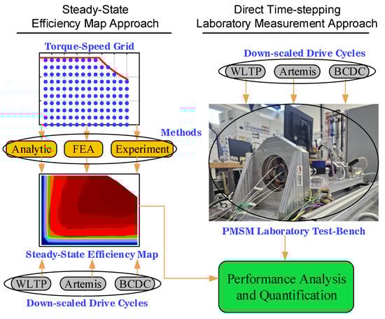
Figure 1.
Flowchart of the study.
2.1. Efficiency Map Approach
This approach usually starts with the selection of different torque–speed grid points (grid density) that are simulated (either analytically or with FEA) or experimentally measured [26,29,40,41]. Evenly distributed grid points are considered with torque points between 0 Nm and 0.14 Nm and speed points between 500 rpm and 7100 rpm. Six different grid densities are considered for the analysis as shown in Figure 2. It should be noted that only the grid points that fall under the operational capability of the laboratory test bench are considered. For simulation-based approaches (a detailed description of each model is provided in the following; see Section 2.1.1 and Section 2.1.2), associated losses and mechanical output power are computed for each OP, and the efficiency at that OP is calculated as defined in (1) [42,43,44]. It is important to note that, for operating points in the generating region (i.e., negative torque and positive speed), the definitions of input and output power are reversed, and the efficiency has been calculated accordingly. In the following sub-sections, different methods for efficiency map approach are explained.
In both simulation methods, copper, iron, and mechanical losses are considered. Additional losses such as those in the magnets and the converter (e.g., PWM switching and conduction losses) are excluded, as their influence on the overall results is considered of minor importance in the context of this study. Details of both the analytic and the FEA model are also published; see [27,36,38]. All simulations and measurements are conducted at room temperature.
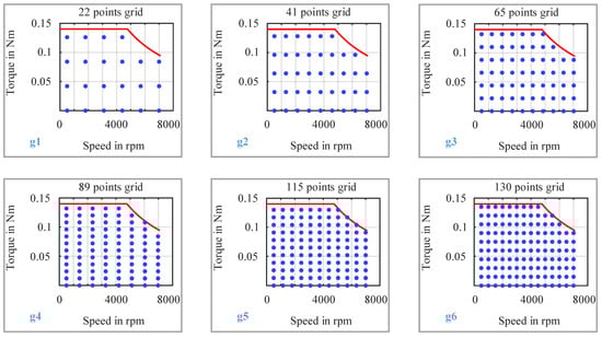
Figure 2.
Different torque–speed grid densities considered for the efficiency-map-based analysis.
2.1.1. Analytic
For the analytic method, a MATLAB® R2023b script-based model is developed to compute the total losses corresponding to each motor OP across varying grid densities. The corresponding current magnitude for each OP is pre-determined using the maximum torque per ampere (MTPA) control strategy and subsequently employed in the loss calculations. Mechanical losses are modeled using a curve-fitted empirical equation as a function of motor speed, derived from experimental no-load measurement data. Core losses are modeled using common frequency domain models (such as Bertotti model [45]) that incorporate loss coefficients for eddy current, hysteresis, and excess losses. These loss coefficients are also derived using curve-fitting tools (e.g., MATLAB® curve-fitting tool [46]) using laboratory measurement data. The PMSM no-load and load measurement data as well as equivalent circuit parameters are available in [38].
2.1.2. FEA
For the FEA method, a high-fidelity electromagnetic model of the PMSM as shown in Figure 3, is developed within a commercial software JMAG® 23.0 [47]. Each torque–speed operating point is simulated as an individual case, and the associated losses are computed accordingly. In addition to the ohmic and core losses obtained directly from the FEA simulations, the associated mechanical losses are incorporated to determine the efficiency at each OP. The simulations are carried out using a model with a mesh resolution of 1.5 mm (as presented in Section 3.4.2, this mesh size gives a perfect balance of computation time and accuracy), and each case is simulated over a full electrical cycle to ensure accurate loss characterization.
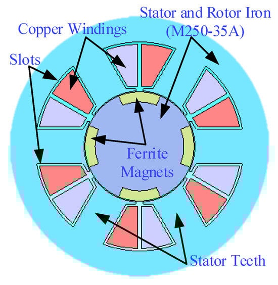
Figure 3.
A 2D schematic of the PMSM FEA model.
2.1.3. Experiment
In steady-state experimental method, all torque–speed OPs are measured in the laboratory. A laboratory test bench setup including a simplified control schematic is shown in Figure 4. A summary of the laboratory measurement equipment and the corresponding accuracies is presented in Table A2 in Appendix A. Each OP is measured for a duration of 30 sec. A transition time of 1 sec is allocated between consecutive OPs to ensure that steady-state conditions are achieved before the measurement period begins. A similar approach is also presented in [26]. For each OP, input electrical power and output mechanical power are measured, and the OP efficiency is calculated as defined in (2).
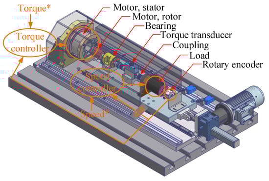
Figure 4.
A 3D schematic of the PMSM laboratory test bench. The orange lines represent the simplified control schematic. The system integrates both efficiency-map-based computations and direct time-stepping laboratory measurements. The motor under test is torque-controlled and the load motor is speed-controlled. * denotes that the values are commanded.
2.2. Time-Stepping Approach
For the time-stepping approach, down-scaled transient drive cycles are directly measured in the laboratory. Both the speed and torque time profiles of the drive cycles are used as inputs. A complete control block diagram of the laboratory test setup used for testing these time-dependent drive profiles is shown in Figure 5. As illustrated, the torque-time profile is applied to the motor under test (referred to as MOTOR), while the speed-time profile is provided to the load motor (referred to as LOAD).
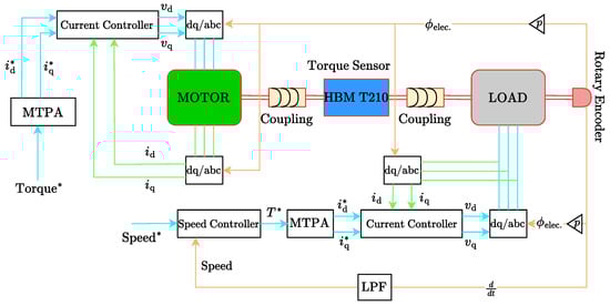
Figure 5.
Complete control block diagram of the PMSM laboratory test bench used for drive cycle time-stepping measurements. Real-time control, data acquisition, and torque–speed profile tracking are implemented to ensure accurate replication of drive scenarios. The speed in fed back using a low pass filter (LPF) with a time constant of . * denotes that the values are commanded.
A cascaded control structure is implemented for speed regulation, comprising inner current control loops and an outer speed control loop. For torque control, the MTPA control strategy is employed. A torque sensor placed between the MOTOR and LOAD captures the shaft torque. A rotary encoder provides position feedback. All measurements are recorded using an HBM Gen3i device [48], operating at a sampling rate of 2 MS/s. For each time step in the torque and speed profiles, both input and output power are measured, allowing the instantaneous efficiency to be calculated as defined in (3). Unlike the steady-state approach, the time-stepping transient measurement method revealed a few instances, particularly in low-torque and regenerative operating regions, where the direction of power flow could not be clearly determined. In such cases, efficiency is undefined and has therefore been conservatively assigned a value of zero.
3. Results and Discussions
The study results from both approaches discussed above are presented and analyzed in detail. These results include drive cycle energy conversion efficiency, energy losses, and a thorough quantification of the findings.
3.1. Efficiency Map Approach
Example efficiency maps and the corresponding WLTP cycle efficiency plots (obtained through efficiency maps as LUTs) for three different methods (Analytic, FEA, and Experiment) presented above on the steady-state efficiency map approach are illustrated in Figure 6a–f, respectively. To visualize the differences in OP efficiency obtained through steady-state simulations and measurements, the efficiency difference heat maps are generated. The results for a 130-point grid (g6), as an example, are presented in Figure 7a–c. The most significant discrepancies occur in the low-speed, low- to high-torque region, as well as in the high-speed, low-torque region. In these regions, the modeled mechanical losses (especially the frictional losses) could not fully capture the change across different motor OPs, leading to higher accuracy compromises in the simplified, fast models. Additionally, the small discrepancies between the reference and the measured OPs during measurements further contribute to these deviations; see Section 3.4.5. The average deviation between analytically and experimentally determined efficiency values is ∼3.5%, while this deviation between the efficiency values obtained through FEA and experiment is around 3.8%. The average difference in the OP efficiencies from two simulation methods (FEA and Analytic) is below 1.5%.
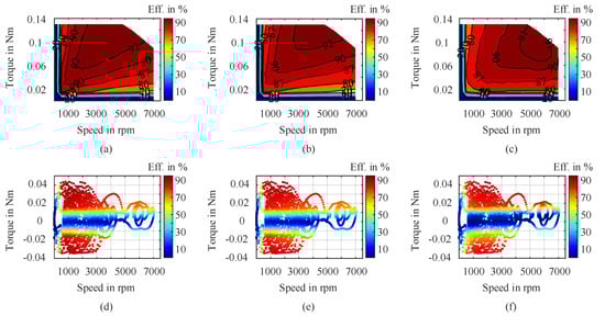
Figure 6.
Efficiency maps and corresponding efficiency plots of the PMSM during down−scaled WLTP drive cycle OPs (with BMW i3), determined from steady−state LUT−based analysis: (a,d) through FEA model, (b,e) through analytic model, (c,f) through experiment; interpolations are based on the 130−point grid (g6) for each map.
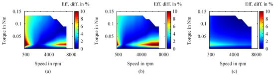
Figure 7.
Efficiency difference heat maps of torque–speed OP efficiencies determined through simulations and measurements: (a) FEA—Experiment, (b) Analytic—Experiment, (c) FEA—Analytic. The example results are shown for the 130-point grid (g6).
3.2. Time-Stepping Approach
The full time-stepping measurement results of the down-scaled WLTP drive cycle (with BMW i3) are presented in Figure 8a–d, where measured speed, torque, input and output power, and calculated efficiency time profiles are shown. All other drive cycles measurement results, along with additional PMSM design and measurement data, are published and made openly accessible in [38]. Direct comparison of performance of drive cycle OPs (down-scaled WLTP with BMW i3) between the efficiency map approach and direct time-stepping measurement approach yields an average mean absolute error (MAE) of 8% to 10%. The complete data of point-wise performance comparison (for all 18 analysis cases) is presented in Table A3 in Appendix B.
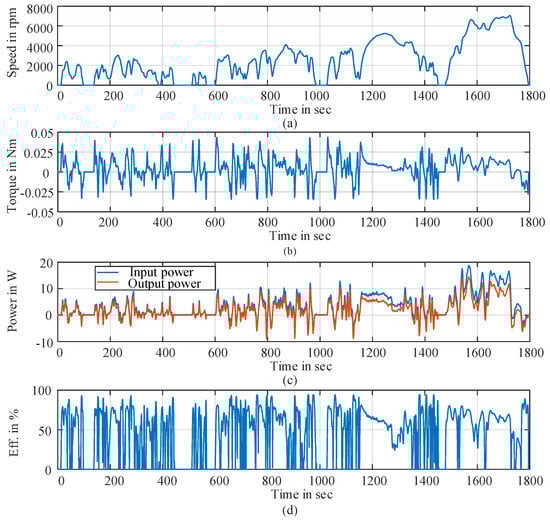
Figure 8.
Laboratory measurement results of full down-scaled WLTP drive cycle (with BMW i3): (a) speed−time profile, (b) torque−time profile, (c) input and output power−time profiles, (d) calculated efficiency-time profile.
3.3. Energy Conversion Efficiency and Loss Analysis
To better understand the steady-state efficiency map method across different torque–speed grid densities, as well as the direct time-stepping method, full drive cycle energy conversion efficiencies and the associated energy losses are analyzed. Both input energy (the total electrical energy required to operate the motor, ) and output energy (total mechanical energy required to operate the cycle, ) are computed as the cumulative sum of the products of the respective power values and their corresponding time steps () over the down-scaled drive cycles, as defined in (4) and (5).
Shown in Figure 9 and Figure 10 are the drive cycle energy efficiency and energy loss bar charts, respectively. The results shown correspond to the down-scaled drive cycles with the BMW i3. The corresponding results for the Smart EQ are provided in Table A4 and Table A5, respectively, both in Appendix B. In general, increasing the grid density of the efficiency map is expected to enhance drive cycle performance predictions. However, as observed in this study, an optimal grid density and grid point distribution exist for each modeling approach, e.g., g4 for FEA/analytic methods and g6 for the experimental method, as explained further down in Section 3.4.5. This optimal grid density and grid point distribution yield steady-state performances closest to those of the transient time-stepping results. Beyond this optimal point, further refinement of the grid does not improve the accuracy of performance prediction. Instead, it may even increase the difference between the steady-state and transient results. This behavior is attributed to the grid density and grid point distribution, where interpolation-induced effects outweigh the benefits of finer resolution. Up to the optimum grid density, this behavior is mainly attributed to the effect of the interpolation which decreases with increasing grid density. Beyond this, it is attributed to the influence of transient effects, but further research is needed to fully understand these observations. Furthermore, differences between the realized and theoretical grid points will also affect the results. Below, in Section 3.4.1, we analyze and explain the effects of different grid point placements on the drive cycle performance prediction using the same grid density. A clear trade-off exists between computational time and accuracy, necessitating careful selection of both grid density and grid point distribution, to optimize the performance prediction from the steady-state efficiency-map-based approach when compared with time-stepping transient measurements.
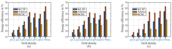
Figure 9.
Drive cycle energy conversion efficiencies from steady-state efficiency map based approach and direct laboratory time-stepping measurements . Efficiency maps as LUTs are constructed and results are shown for different torque–speed grid points (grid × 2 meaning motoring/generating regions, respectively) using (a) FEA method, (b) Analytic method, (c) Experiment method. Drive cycle total output energy as measured in the laboratory: WLTP = 2.96 kJ, Artemis = 5.37 kJ, and BCDC = 1.45 kJ.
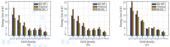
Figure 10.
Influence of the no. of grid points on the efficiency maps’ predictive performance. The figures show the energy loss of the drive cycles as determined from efficiency maps and by direct time-stepping measurements in the laboratory , all for the mid-size car (BMW i3). Efficiency maps as LUTs are constructed for different torque–speed grid points (grid × 2 meaning motoring/generating regions, respectively) using (a) FEA method, (b) Analytic method, (c) Experiment method. Drive cycle total input energy as measured in the laboratory: WLTP = 5.46 kJ, Artemis = 8.53 kJ, and BCDC = 3.65 kJ.
A visual representation of the total input energy-time profile during PMSM drive cycle operation (down-scaled WLTP with BMW i3) computed using both approaches (efficiency map and time-stepping) is presented in Figure 11. As it can be seen, the efficiency-map-based approach consistently overestimates the required electrical input energy. The total input energy difference between two approaches is around 1.4 kJ for WLTP drive cycle (with BMW i3), which is roughly 26% of the input energy obtained from direct time-stepping measurements. For all studied down-scaled drive cycles, this difference varies between 20% and 30%.
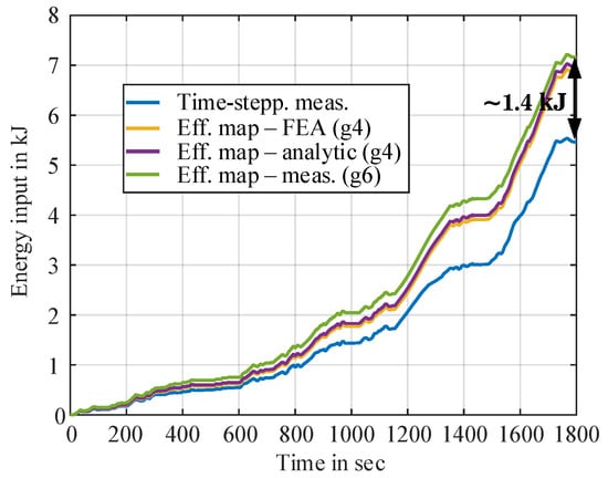
Figure 11.
Total input energy measured or simulated during down-scaled WLTP drive cycle (with BMW i3) operation using different approaches. For the steady-state efficiency-map-based analysis, results are presented only for the optimal grid density identified among the grid densities evaluated.
3.4. Results Quantification
A comprehensive quantification of the results from both study approaches is provided in the following sections.
3.4.1. Quantification of Grid Interpolation Effects
For a given grid density, an influence of placement of torque–speed grid points on the grid interpolation error is studied and quantified. To study this, a grid density of 100 torque–speed grid points (torque points between 0 Nm and 0.14 Nm and speed points between 0 rpm and 7500 rpm) are analytically simulated for their performance. Six different grid placement variations in these points are considered. Subsequently, efficiency maps are generated for each placement, and the performance of the PMSM OPs for a given drive cycle is evaluated using these maps as LUTs. As shown in Figure 12, Grid A has uniformly distributed torque–speed points ; Grid B consists of more torque points and less speed points ; Grid C consists of less torque points and more speed points ; and Grid D, Grid E, and Grid F have a non-uniform torque–speed distribution with quadratic spacing for torque and uniform spacing for speed, uniform spacing for torque and quadratic spacing for speed, and quadratic spacing for torque and quadratic spacing for speed, respectively. As presented, Grid C gives the highest energy loss in comparison to other grid groups. This means the grid interpolation is more sensitive to torque placement. Evidently, the operating regions of drive cycles are more densely populated at low speeds with a wide range of torques. This indicates that copper losses, which directly correspond to torque values, have a greater impact on motor performance in these regions than other types of losses. Since Grid C contains fewer torque points, interpolation occurs over larger distances between points, leading to correspondingly larger differences. Grid D and Grid F, where the torque points are quadratically spaced, predict the energy loss metrics more closer to the time-stepping measurements. As a result, depending on how the grid points are placed, the same grid density influences the drive cycle performance prediction metrics (on the efficiency map approach) by a factor of ∼1/3.
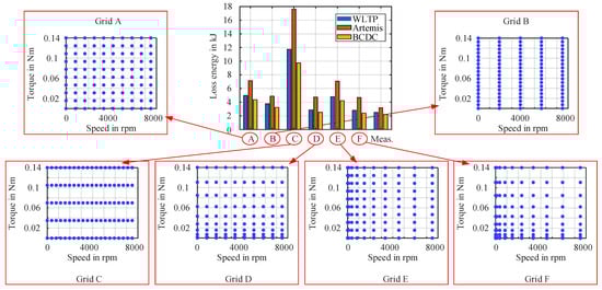
Figure 12.
Quantification of interpolation effects associated with torque–speed grid points under different placement strategies. Plot shows loss energies of different down-scaled drive cycles (with BMW i3), obtained from map-based analyses using various grid points placement and from direct time-stepping laboratory measurements.
3.4.2. Quantification of FEA Mesh Size, Time–Accuracy Trade-Offs
Several PMSM OPs are simulated using the FEA model with varying mesh element sizes, and the corresponding motor performance metrics are computed. These simulation results are then compared with the corresponding experimental measurements. Each simulation is performed over one full electrical period. As shown in Figure 13, the figure illustrates the impact of mesh element size on the PMSM performance accuracy for an example operating point at 0.042 Nm and 1800 rpm. The error is presented relative to the corresponding laboratory measurements. As observed, there is a clear trade-off between accuracy and computational time: smaller mesh elements improve accuracy but increase computation time. Notably, the relationship among mesh size, accuracy, and computational effort is non-linear, highlighting the need for careful mesh size selection to achieve better time–accuracy metrics. Moreover, Figure 14 illustrates the relationship between torque–speed grid density and time–accuracy trade-offs for various FEA-simulated grid resolutions, comparing efficiency-map-based drive cycle performance predictions to direct time-stepping measurements. As shown, a clear trade-off exists between computational time and accuracy, with an optimal grid density giving the best performance metrics for all drive cycles.
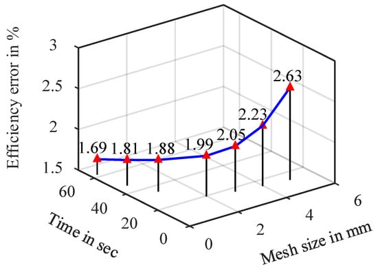
Figure 13.
Quantification of the FEA model in terms of mesh size, computational time, and accuracy for evaluating the performance of a PMSM OP. The results are obtained from simulations at an OP with a torque of 0.042 Nm and a speed of 1800 rpm.
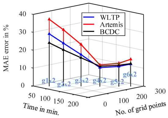
Figure 14.
Trade-off between no. of evenly spaced FEA-simulated grid points (grid × 2 meaning motoring/generating regions, respectively) for efficiency map determination, simulation time, and drive cycle efficiency prediction. Results are shown in terms of the MAE where reference [49] is the direct time-stepping laboratory measurements for corresponding down-scaled drive cycles (with BMW i3).
3.4.3. Quantification on Effects of Temperature
The effect of temperature on the PMSM efficiency map (and ultimately on the drive cycle performance prediction) is simulated and analyzed. An increase in temperature (particularly in the windings and magnets) increases the related losses and reduces the motor’s overall efficiency, thereby impacting the accuracy of the drive cycle performance.
As shown in Figure 15, increasing the steady-state temperature from 20 °C to 100 °C mainly impacts the medium- to high-torque–speed regions, making the map appear as if it expands from bottom to top as temperature increases. As observed, the 92% efficiency contour observed at 20 °C disappears at 100 °C, indicating a substantial efficiency loss at elevated temperatures. This highlights the significant influence of temperature on the efficiency prediction and underscores the importance of evaluating or correcting efficiency maps according to the thermal conditions present during drive cycle measurements.
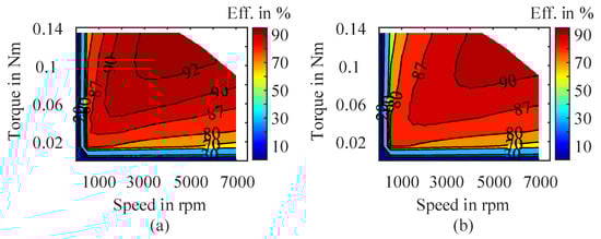
Figure 15.
Simulated steady−state efficiency maps of the PMSM at different temperatures: (a) 20 °C, (b) 100 °C; interpolations are based on the 130−point grid (g6) for each map.
However, since all operating points of the down-scaled PMSM drive cycles lie in low-torque regions (typically below 50% of the maximum torque), thermal effects during these operations are negligible. Performance comparisons using simulated efficiency maps across these temperatures revealed minimal variation, with overall efficiency degradation from 20 °C to 100 °C being less than 0.5%.
Low thermal utilization during down-scaled drive cycles operation is further understood during laboratory measurements. Shown in Figure 16 are the temperature rise in different motor parts during laboratory testing of the down-scaled WLTP drive cycle (with BMW i3). As observed, the temperature rise was significantly lower, indicating low thermal utilization due to the down-scaling to the smaller laboratory settings.
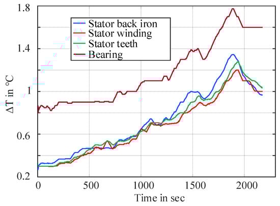
Figure 16.
Measured temperature rise () of selected parts of the laboratory PMSM during down-scaled WLTP drive cycle (with BMW i3) operation.
The limited temperature rise, compared with typically anticipated values, also reflects the inherent characteristics of the applied drive cycles down-scaling method. This behavior is attributed to the simultaneous down-scaling of two different physics: electromagnetic and thermal. With electric machines, the electromagnetic properties generally scale with the machine volume, whereas the thermal properties rather scale with the surface available for cooling. This suggests the importance of investigating scaling techniques capable of replicating the thermal behavior of real EV motors in small laboratory settings also.
3.4.4. Computational Efficiency of Methods
To study the computational efficiency of the efficiency-map-based approach, the total computational time of different methods (Analytic, FEA, Experiment) is considered. It includes simulation/measurement time for an example grid density (g4), efficiency map creation, and drive cycle performance calculation. For direct time-stepping measurements, it includes the total time required for measurements and drive cycle performance calculation. This is summarized in Table 1. Efficiency-map-based approach is fast and can be accurate enough given the optimal grid density as well as grid point placement. Direct time-stepping measurement approach on the other hand can be time-consuming though inherently accurate.

Table 1.
Simulation and measurement times of different approaches on drive cycle performance computation.
3.4.5. Influence of Error Sources
As the study shows, irrespective of the specific method applied, the efficiency-map-based steady-state approach consistently overestimates the total input energy required over a drive cycle, resulting in an artificially optimistic assessment of energy efficiency for the example case PMSM. This overestimation stems mainly from various source of errors as presented in Table 2. It results from the neglect of dynamic drive behavior and the reliance on linear interpolation between grid points. Additionally, inaccuracies in loss modeling (particularly mechanical losses) constitute one of the dominant contributors.
Table 2.
Degrees of influence of the difference error sources on the drive cycle efficiency prediction using efficiency maps as LUTs across PMSM models as derived from this study (aggregated view). For a general overview on the different types of losses and their impacts on motor performance, see [9,44,50,51,52,53,54].
Additionally, in both the steady-state-based FEA and the experimental approach, there are differences between the measured or simulated grid points and the reference grid points, as shown in Figure 17. The root-mean-squared (RMS) torque error () relative to the reference grid points (g6) is 0.0020 Nm for the corresponding FEA-simulated points, while it is 0.0031 Nm for the corresponding measured points. This difference results in a drive cycle performance prediction error of less than 1% in FEA (as can be seen, most of the differences occur in the high-torque regions, outside of the typical operating range of the drive cycles) and approximately 2 to 5% for steady-state measurements (differences are seen through out the grid) when compared with direct time-stepping measurements. In the experimental method, although the grid density remains the same, interpolation is performed between a different set of grid points compared to the reference grid points. This likely contributed to g6 being the optimal grid density among the grid densities considered, providing steady-state performance prediction metrics closest to the time-stepping measurements. In contrast, for the simulation-based methods (FEA and analytical), the optimal grid density is found to be g4. Therefore, establishing the optimal grid density requires balancing computational efficiency with modeling and predictive accuracy to ensure that the steady-state maps represent the transient behavior as closely as possible.
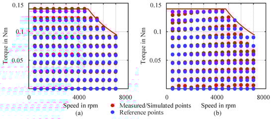
Figure 17.
Visual difference between the reference and measured/simulated torque–speed OPs for steady-state efficiency map approach with (a) FEA method, (b) Experiment method. An example case of 130-point grid (g6) is presented.
4. Conclusions
This study presents a comprehensive study on the drive cycle performance analysis of a small laboratory-scale PMSM using two distinct approaches. Analytic, FEA, and experimental steady-state efficiency-map-based methods are studied against direct laboratory time-stepping measurements for several down-scaled drive cycles.
The findings indicate that most discrepancies between the efficiency-map-based predictions and time-stepping measurements occur in low-speed regions with low-to-high torque and at high speeds with low torque. Notably, the steady-state map approach consistently overestimates the required energy input across all tested grid densities and drive cycles. Although increasing grid density improves prediction accuracy, there exists an optimal combination of grid density and grid distribution that provides the most accurate results.
Additionally, the distribution of the grid points significantly influences the drive cycle performance predictions, with variations of up to one-third compared to transient measurements, depending on the chosen grid configuration. Furthermore, in the case of the steady-state methods, the differences between the reference and measured grid points also contributed to the identification of a different optimal grid density.
Thermal effects are considered negligible in this study due to the down-scaling of drive cycles for the small laboratory setup. The motor’s size, test bench configuration, and low power rating limited its thermal loading and utilization. This suggests that thermal effects need to be accounted for separately when down-scaling electro-mechanical characteristics down to the laboratory conditions. In high-power real-world motor applications, the rise in temperature and its influence on overall motor performance, particularly its effects on windings, magnets, and other related components, are critical factors that cannot be neglected.
Finally, efficiency-map-based approach can still be accurate enough provided that an optimal grid density or grid combination is properly simulated or measured. On the other hand, direct time-stepping measurements are resource-intensive though inherently accurate. A promising way forward lies in data-driven or high-fidelity hybrid models that are accurate and computationally efficient.
Author Contributions
Conceptualization, P.K.D., K.H. and A.M.; Measurements, P.K.D. and R.S.; Investigation and Validation, P.K.D. and K.H.; Writing—original draft, P.K.D.; Supervision, A.M. All authors have read and agreed to the published version of the manuscript.
Funding
This work is partially supported by the joint Collaborative Research Centre CREATOR (DFG: Project-ID 492661287/TRR 361; FWF: 10.55776/F90) at TU Darmstadt, TU Graz and JKU Linz. For the purpose of open access, the author has applied a CC BY public copyright license to any Author Accepted Manuscript version arising from this submission.
Data Availability Statement
A complete set of PMSM data package that provides all the required information in terms of design parameters (electrical, mechanical, geometry, windings, materials, etc.) and measurement results (no-load, load, and different transient drive cycles) are published with open access and available in [38].
Acknowledgments
ChatGPT 3.5 [55] has been used for editing and grammar enhancement of the paper. The paper has been subsequently edited manually again.
Conflicts of Interest
The authors declare no conflicts of interest.
Appendix A
Table A1.
Vehicle motors and laboratory motor specifications.
Table A1.
Vehicle motors and laboratory motor specifications.
| Specifications of Vehicle Motors [56,57] | ||
|---|---|---|
| Parameters | Values | |
| BMW i3 | Smart EQ | |
| Machine Type | PMSM | PMSM |
| Max. Torque | 250 Nm | 160 Nm |
| Max. Power | 125 kW | 60 kW |
| Rated Speed | 4800 rpm | 3600 rpm |
| Max. Speed | 11,400 rpm | 11,475 rpm |
| Laboratory Motor Specifications [38] | ||
| Motor | Parameters | Values |
| Max. Power | 70 W | |
| Max. Torque | 0.15 Nm | |
| PMSM | Rated Speed | 2000 rpm |
| Max. Speed | 7050 rpm | |
Table A2.
A detail description of the test equipment used for the laboratory measurements.
Table A2.
A detail description of the test equipment used for the laboratory measurements.
| Type of Measurement | Device | Accuracy |
|---|---|---|
| Data recorder | HBM Gen 3i [48] | 2MS/s |
| Torque | HBM T210 [58] | |
| Temperature | RS T & J Type thermocouples [59,60] | °C |
| Rotor position | ECN 413 [61] | |
| Current | LEM IT 60-S [62] | 0.02725% |
| Voltage | HBM Gen 3i equipped with GEN Series GN610 [63] | 0.02% |
Appendix B
Table A3.
The MAE [49] error of efficiencies of the PMSM drive cycle OPs obtained from steady-state efficiency maps as compared to direct time-stepping measurements. Grid densities highlighted in blue represent the optimal configurations, yielding minimal error among the grid densities evaluated.
Table A3.
The MAE [49] error of efficiencies of the PMSM drive cycle OPs obtained from steady-state efficiency maps as compared to direct time-stepping measurements. Grid densities highlighted in blue represent the optimal configurations, yielding minimal error among the grid densities evaluated.
| Approach | Grid | MAE of Drive Cycles OPs | ||
|---|---|---|---|---|
| WLTP | Artemis | BCDC | ||
| Mid-Sized Vehicle (BMW i3) | ||||
| Eff. map (analytic) | g1 | 28.08% | 35.96% | 22.91% |
| g2 | 22.86% | 30.00% | 18.97% | |
| g3 | 16.20% | 21.37% | 14.48% | |
| g4 | 8.40% | 10.00% | 9.73% | |
| g5 | 9.14% | 10.95% | 10.25% | |
| g6 | 10.68% | 13.18% | 11.28% | |
| Eff. map (FEA) | g1 | 28.76% | 36.87% | 23.58% |
| g2 | 23.35% | 30.82% | 19.48% | |
| g3 | 16.46% | 22.12% | 14.76% | |
| g4 | 8.41% | 9.65% | 9.73% | |
| g5 | 9.16% | 10.71% | 10.29% | |
| g6 | 10.14% | 11.98% | 11.00% | |
| Eff. map (experiment) | g1 | 31.69% | 39.47% | 25.32% |
| g2 | 26.08% | 33.05% | 21.22% | |
| g3 | 20.05% | 24.32% | 17.13% | |
| g4 | 12.30% | 10.09% | 12.97% | |
| g5 | 12.50% | 10.25% | 12.98% | |
| g6 | 18.89% | 10.57% | 11.50% | |
| Small-Sized Vehicle (Smart EQ) | ||||
| Eff. map (analytic) | g1 | 27.09% | 33.35% | 21.88% |
| g2 | 22.13% | 26.50% | 18.02% | |
| g3 | 16.26% | 16.56% | 13.68% | |
| g4 | 10.13% | 6.11% | 9.25% | |
| g5 | 10.68% | 6.65% | 9.73% | |
| g6 | 11.85% | 8.26% | 10.66% | |
| Eff. map (FEA) | g1 | 27.77% | 34.45% | 22.49% |
| g2 | 22.60% | 27.48% | 18.45% | |
| g3 | 16.62% | 17.46% | 13.84% | |
| g4 | 10.44% | 5.72% | 9.30% | |
| g5 | 10.97% | 6.34% | 9.80% | |
| g6 | 12.14% | 8.32% | 10.77% | |
| Eff. map (experiment) | g1 | 30.66% | 36.70% | 24.14% |
| g2 | 25.25% | 29.09% | 20.10% | |
| g3 | 19.87% | 18.73% | 16.15% | |
| g4 | 13.11% | 7.64% | 12.25% | |
| g5 | 13.32% | 7.25% | 12.13% | |
| g6 | 18.70% | 17.76% | 16.21% | |
Table A4.
PMSM drive cycle energy efficiencies () obtained from grid-based efficiency maps and direct time-stepping measurements. Drive cycle total output energy () as measured in the laboratory: = , = , and = . Highlighted in blue are the corresponding optimal grid densities.
Table A4.
PMSM drive cycle energy efficiencies () obtained from grid-based efficiency maps and direct time-stepping measurements. Drive cycle total output energy () as measured in the laboratory: = , = , and = . Highlighted in blue are the corresponding optimal grid densities.
| Approach | Grid | Drive Cycles Energy Efficiency | ||
|---|---|---|---|---|
| WLTP | Artemis | BCDC | ||
| Small-Sized Vehicle (Smart EQ) | ||||
| Time-stepping meas. | - | 56.54% | 65.84% | 39.06% |
| Eff. map (analytic) | g1 | 16.54% | 27.00% | 10.90% |
| g2 | 21.10% | 33.96% | 14.02% | |
| g3 | 28.30% | 45.62% | 19.53% | |
| g4 | 40.40% | 59.40% | 29.00% | |
| g5 | 38.62% | 58.63% | 27.80% | |
| g6 | 36.10% | 56.43% | 25.53% | |
| Eff. map (FEA) | g1 | 15.81% | 25.80% | 10.38% |
| g2 | 20.35% | 32.78% | 13.50% | |
| g3 | 27.72% | 44.50% | 19.11% | |
| g4 | 40.68% | 60.30% | 29.41% | |
| g5 | 39.05% | 59.36% | 28.04% | |
| g6 | 35.84% | 56.56% | 25.57% | |
| Eff. map (experiment) | g1 | 13.24% | 22.77% | 7.35% |
| g2 | 16.19% | 29.96% | 9.24% | |
| g3 | 22.09% | 41.61% | 12.78% | |
| g4 | 35.32% | 60.60% | 19.95% | |
| g5 | 34.73% | 59.26% | 19.54% | |
| g6 | 25.13% | 42.57% | 13.35% | |
Table A5.
PMSM drive cycles loss energies () obtained from grid-based efficiency maps using different methods. Drive cycle total output energy () as measured in the laboratory: = , = , and = . Highlighted in blue are the corresponding optimal grid densities.
Table A5.
PMSM drive cycles loss energies () obtained from grid-based efficiency maps using different methods. Drive cycle total output energy () as measured in the laboratory: = , = , and = . Highlighted in blue are the corresponding optimal grid densities.
| Approach | Grid | Drive Cycles Energy Loss in kJ | ||
|---|---|---|---|---|
| WLTP | Artemis | BCDC | ||
| Small-Sized Vehicle (Smart EQ) | ||||
| Time-stepping meas. | - | 2.67 kJ | 3.54 kJ | 2.82 kJ |
| Eff. map (analytic) | g1 | 17.50 kJ | 18.48 kJ | 14.80 kJ |
| g2 | 13.01 kJ | 13.30 kJ | 11.08 kJ | |
| g3 | 8.80 kJ | 8.14 kJ | 6.05 kJ | |
| g4 | 5.13 kJ | 4.67 kJ | 4.43 kJ | |
| g5 | 5.50 kJ | 4.82 kJ | 4.70 kJ | |
| g6 | 6.15 kJ | 5.27 kJ | 5.26 kJ | |
| Eff. map (FEA) | g1 | 18.47 kJ | 19.65 kJ | 15.60 kJ |
| g2 | 13.58 kJ | 14.01 kJ | 11.57 kJ | |
| g3 | 9.05 kJ | 8.52 kJ | 7.65 kJ | |
| g4 | 5.06 kJ | 4.50 kJ | 4.33 kJ | |
| g5 | 5.41 kJ | 4.67 kJ | 4.63 kJ | |
| g6 | 6.21 kJ | 5.24 kJ | 5.26 kJ | |
| Eff. map (experiment) | g1 | 22.73 kJ | 23.17 kJ | 22.76 kJ |
| g2 | 17.95 kJ | 15.97 kJ | 17.75 kJ | |
| g3 | 12.23 kJ | 9.59 kJ | 12.33 kJ | |
| g4 | 6.35 kJ | 4.44 kJ | 7.25 kJ | |
| g5 | 6.52 kJ | 4.70 kJ | 7.43 kJ | |
| g6 | 10.33 kJ | 9.22 kJ | 11.72 kJ | |
References
- Blanco, S. Toyota, Mazda, Subaru Agree Carbon is ‘Enemy’ with Internal Combustion Engine Announcement. 2024. SAE 2 International. Available online: https://www.sae.org/site/news/2024/05/toyota-internal-combustion-future-engines (accessed on 8 September 2025).
- Rémont, L. Why Electrification Is So Important to the Energy Transition. 2025. World Economic Forum. Available online: https://www.weforum.org/stories/2025/01/why-electrification-important-energy-transition/ (accessed on 8 September 2025).
- Liu, C.; Chau, K.T.; Lee, C.H.T.; Song, Z. A Critical Review of Advanced Electric Machines and Control Strategies for Electric Vehicles. Proc. IEEE 2021, 109, 1004–1028. [Google Scholar] [CrossRef]
- Sayed, E.; Abdalmagid, M.; Pietrini, G.; Sa’adeh, N.M.; Callegaro, A.D.; Goldstein, C.; Emadi, A. Review of Electric Machines in More-/Hybrid-/Turbo-Electric Aircraft. IEEE Trans. Transp. Electrif. 2021, 7, 2976–3005. [Google Scholar] [CrossRef]
- Huynh, T.A.; Chen, P.H.; Hsieh, M.F. Analysis and Comparison of Operational Characteristics of Electric Vehicle Traction Units Combining Two Different Types of Motors. IEEE Trans. Veh. Technol. 2022, 71, 5727–5742. [Google Scholar] [CrossRef]
- Huynh, T.; Hsieh, M.F. Performance Analysis of Permanent Magnet Motors for Electric Vehicles (EV) Traction Considering Driving Cycles. Energies 2018, 11, 1385. [Google Scholar] [CrossRef]
- Gobbi, M.; Sattar, A.; Palazzetti, R.; Mastinu, G. Traction motors for electric vehicles: Maximization of mechanical efficiency—A review. Appl. Energy 2024, 357, 122496. [Google Scholar] [CrossRef]
- Ozer, K.; Yilmaz, M. Design and Optimization of IPMSM for Enhanced Efficiency, Cost Reduction, and Performance in Light Electric Vehicles. IEEE Access 2025, 13, 80621–80636. [Google Scholar] [CrossRef]
- Ran, Z.; Zhu, Z.Q.; Chen, Z.; Younkins, M.; Farah, P. Novel System-Level Driving-Cycle-Oriented Design Co-Optimization of Electrical Machines for Electrical Vehicles. IEEE Access 2024, 12, 131734–131749. [Google Scholar] [CrossRef]
- Pyrhönen, J.; Jokinen, T.; Hrabovcová, V. Design of Rotating Electrical Machines; Wiley: Hoboken, NJ, USA, 2013. [Google Scholar]
- Grunditz, E.A.; Thiringer, T.; Saadat, N. Acceleration, Drive Cycle Efficiency, and Cost Tradeoffs for Scaled Electric Vehicle Drive System. IEEE Trans. Ind. Appl. 2020, 56, 3020–3033. [Google Scholar] [CrossRef]
- Fatemi, A.; Demerdash, N.A.O.; Nehl, T.W.; Ionel, D.M. Large-Scale Design Optimization of PM Machines Over a Target Operating Cycle. IEEE Trans. Ind. Appl. 2016, 52, 3772–3782. [Google Scholar] [CrossRef]
- Diao, K.; Sun, X.; Lei, G.; Bramerdorfer, G.; Guo, Y.; Zhu, J. System-Level Robust Design Optimization of a Switched Reluctance Motor Drive System Considering Multiple Driving Cycles. IEEE Trans. Energy Convers. 2021, 36, 348–357. [Google Scholar] [CrossRef]
- Praslicka, B.; Ma, C.; Taran, N. A Computationally Efficient High-Fidelity Multi-Physics Design Optimization of Traction Motors for Drive Cycle Loss Minimization. IEEE Trans. Ind. Appl. 2023, 59, 1351–1360. [Google Scholar] [CrossRef]
- Roshandel, E.; Mahmoudi, A.; Soong, W.L.; Kahourzade, S. Optimal Design of Induction Motors Over Driving Cycles for Electric Vehicles. IEEE Trans. Veh. Technol. 2023, 72, 15548–15562. [Google Scholar] [CrossRef]
- Hwang, S.W.; Ryu, J.Y.; Chin, J.W.; Park, S.H.; Kim, D.K.; Lim, M.S. Coupled Electromagnetic-Thermal Analysis for Predicting Traction Motor Characteristics According to Electric Vehicle Driving Cycle. IEEE Trans. Veh. Technol. 2021, 70, 4262–4272. [Google Scholar] [CrossRef]
- Fan, D.; Zhu, X.; Quan, L.; Han, P.; Xiang, Z.; Wu, J. Driving Cycle Design Optimization of Less-Rare-Earth PM Motor Using Dimension Reduction Method. IEEE Trans. Energy Convers. 2023, 38, 1614–1625. [Google Scholar] [CrossRef]
- Abdel-Wahed, A.T.; Ullah, Z.; Abdel-Khalik, A.S.; Hamad, M.S.; Ahmed, S.; Elmalhy, N. Drive Cycle-Based Design with the Aid of Data Mining Methods: A Review on Clustering Techniques of Electric Vehicle Motor Design with a Case Study. IEEE Access 2023, 11, 115775–115797. [Google Scholar] [CrossRef]
- Mahmouditabar, F.; Vahedi, A.; Takorabet, N. Robust Design of BLDC Motor Considering Driving Cycle. IEEE Trans. Transp. Electrif. 2024, 10, 1414–1424. [Google Scholar] [CrossRef]
- Bhaktha, B.S.; Jose, N.; Vamshik, M.; Pitchaimani, J.; Gangadharan, K.V. Driving Cycle-Based Design Optimization and Experimental Verification of a Switched Reluctance Motor for an E-Rickshaw. IEEE Trans. Transp. Electrif. 2024, 10, 9959–9974. [Google Scholar] [CrossRef]
- Williamson, S.S.; Emadi, A.; Rajashekara, K. Comprehensive Efficiency Modeling of Electric Traction Motor Drives for Hybrid Electric Vehicle Propulsion Applications. IEEE Trans. Veh. Technol. 2007, 56, 1561–1572. [Google Scholar] [CrossRef]
- Jun, S.B.; Kim, C.H.; Cha, J.; Lee, J.H.; Kim, Y.J.; Jung, S.Y. A Novel Method for Establishing an Efficiency Map of IPMSMs for EV Propulsion Based on the Finite-Element Method and a Neural Network. Electronics 2021, 10, 1049. [Google Scholar] [CrossRef]
- Roshandel, E.; Mahmoudi, A.; Kahourzade, S.; Soong, W.L. Efficiency Maps of Electrical Machines: A Tutorial Review. IEEE Trans. Ind. Appl. 2023, 59, 1263–1272. [Google Scholar] [CrossRef]
- Ferrari, S.; Ragazzo, P.; Dilevrano, G.; Pellegrino, G. Flux and Loss Map Based Evaluation of the Efficiency Map of Synchronous Machines. IEEE Trans. Ind. Appl. 2023, 59, 1500–1509. [Google Scholar] [CrossRef]
- Stiscia, O.; Rubino, S.; Vaschetto, S.; Cavagnino, A.; Tenconi, A. Accurate Induction Machines Efficiency Mapping Computed by Standard Test Parameters. IEEE Trans. Ind. Applicat. 2022, 58, 3522–3532. [Google Scholar] [CrossRef]
- Bojoi, R.; Armando, E.; Pastorelli, M.; Lang, K. Efficiency and loss mapping of AC motors using advanced testing tools. In Proceedings of the 2016 XXII International Conference on Electrical Machines (ICEM), Lausanne, Switzerland, 4–7 September 2016; pp. 1043–1049. [Google Scholar] [CrossRef]
- Dhakal, P.K.; Heidarikani, K.; Seebacher, R.; Muetze, A. Baseline Determination for Drive Cycle Performance Analysis of Permanent Magnet Synchronous Motors. In Proceedings of the 2023 IEEE Transportation Electrification Conference and Expo, Asia-Pacific (ITEC Asia-Pacific), Chiang Mai, Thailand, 28 November–1 December 2023; pp. 1–6. [Google Scholar] [CrossRef]
- Heidarikani, K.; Dhakal, P.K.; Seebacher, R.; Muetze, A. Baseline Determination for Drive Cycle Performance Analysis of Induction Motors. In Proceedings of the 2023 IEEE Transportation Electrification Conference and Expo, Asia-Pacific (ITEC Asia-Pacific), Chiang Mai, Thailand, 28 November–1 December 2023; pp. 1–6. [Google Scholar] [CrossRef]
- Kahourzade, S.; Mahmoudi, A.; Soong, W.L.; Ertugrul, N.; Pellegrino, G. Estimation of PM Machine Efficiency Maps From Limited Data. IEEE Trans. Ind. Appl. 2020, 56, 2612–2621. [Google Scholar] [CrossRef]
- Sano, H.; Semba, K.; Suzuki, Y.; Yamada, T. Investigation in the accuracy of FEA Based Efficiency Maps for PMSM traction machines. In Proceedings of the 2022 International Conference on Electrical Machines (ICEM), Valencia, Spain, 5–8 September 2022; pp. 2061–2066. [Google Scholar]
- Mohammadi, M.H.; Lowther, D.A. A Computational Study of Efficiency Map Calculation for Synchronous AC Motor Drives Including Cross-Coupling and Saturation Effects. IEEE Trans. Magn. 2017, 53, 1–4. [Google Scholar] [CrossRef]
- Mahmouditabar, F.; Baker, N.J. Design Optimization of Induction Motors with Different Stator Slot Rotor Bar Combinations Considering Drive Cycle. Energies 2024, 17, 154. [Google Scholar] [CrossRef]
- Gong, Y.; Gneiting, A.; Weigel, S.; Parspour, N.; An, Z. Surrogate Model Based Drive Cycle Modelling and Optimization of Synchronous Reluctance Machines for Electric Vehicles. IEEE Trans. Magn. 2025, 61, 8101906. [Google Scholar] [CrossRef]
- Farajpour, Y.; Chaoui, H.; Kelouwani, S. Cutting-Edge EMS Technologies for EVs and HEVs: Recent Developments and Future Directions. IEEE Access 2025, 13, 130256–130303. [Google Scholar] [CrossRef]
- Narita, K.; Sano, H.; Schneider, N.; Semba, K.; Tani, K.; Yamada, T.; Akaki, R. An Accuracy Study of Finite Element Analysis-based Efficiency Map for Traction Interior Permanent Magnet Machines. In Proceedings of the 2020 IEEE Energy Conversion Congress and Exposition (ECCE), Detroit, MI, USA, 11–15 October 2020; pp. 1722–1726. [Google Scholar]
- Dhakal, P.K.; Heidarikani, K.; Seebacher, R.; Muetze, A. Efficiency Map Versus Time-Stepping Solutions for Drive Cycle Performance Analysis of Permanent Magnet Synchronous Motors. In Proceedings of the 2024 27th International Conference on Electrical Machines and Systems (ICEMS), Fukuoka, Japan, 26–29 November 2024; pp. 336–340. [Google Scholar] [CrossRef]
- Heidarikani, K.; Dhakal, P.K.; Seebacher, R.; Muetze, A. Quantification of Steady-State Efficiency Maps and Time-Stepping Solutions for Drive Cycle Performance Analysis of Induction Motors. In Proceedings of the 2024 27th International Conference on Electrical Machines and Systems (ICEMS), Fukuoka, Japan, 26–29 November 2024; pp. 1–6. [Google Scholar]
- Dhakal, P.K.; Heidarikani, K.; Muetze, A.; Seebacher, R. CREATOR Case: Permanent Magnet Synchronous Motor Data; Graz University of Technology: Graz, Austria, 2024. [Google Scholar] [CrossRef]
- Dhakal, P.K.; Heidarikani, K.; Muetze, A. Down-scaling of drive cycles for experimental drive cycle analyses. In Proceedings of the 12th International Conference on Power Electronics, Machines and Drives (PEMD 2023), Brussels, Belgium, 23–24 October 2023; Volume 2023, pp. 271–276. [Google Scholar] [CrossRef]
- Vanhooydonck, D.; Symens, W.; Deprez, W.; Lemmens, J.; Stockman, K.; Dereyne, S. Calculating energy consumption of motor systems with varying load using iso efficiency contours. In Proceedings of the The XIX International Conference on Electrical Machines—ICEM 2010, Rome, Italy, 6–8 September 2010; pp. 1–6. [Google Scholar] [CrossRef]
- Cheng, Y.; Wang, Y.; Ma, J.; Liu, G.; Li, D.; Qu, R. Fast Evaluation of Driving Cycle Efficiency of Interior Permanent Magnet Synchronous Machines for Electric Vehicles Considering Step-Skewing. In Proceedings of the 2023 IEEE International Electric Machines & Drives Conference (IEMDC), San Francisco, CA, USA, 15–18 May 2023; pp. 1–7. [Google Scholar] [CrossRef]
- Praslicka, B.; Taran, N.; Ma, C. An Ultra-fast Method for Analyzing IPM Motors at Multiple Operating Points Using Surrogate Models. In Proceedings of the 2022 IEEE Transportation Electrification Conference & Expo (ITEC), Anaheim, CA, USA, 15–17 June 2022; pp. 868–873. [Google Scholar] [CrossRef]
- Kong, Y.; Nicola, B.; Lin, M. Loss Functions and Efficiency Model of Permanent Magnet Assisted Synchronous Reluctance Machine. IEEE Trans. Energy Convers. 2023, 38, 53–63. [Google Scholar] [CrossRef]
- Roshandel, E.; Mahmoudi, A.; Kahourzade, S.; Yazdani, A.; Shafiullah, G.M. Losses in Efficiency Maps of Electric Vehicles: An Overview. Energies 2021, 14, 7805. [Google Scholar] [CrossRef]
- Bertotti, G. Hysteresis in Magnetism: For Physicists, Materials Scientists, and Engineers; Academic Press: Cambridge, MA, USA, 1998. [Google Scholar]
- MathWorks. Curve Fitting Toolbox. 2025. Available online: https://www.mathworks.com/products/curvefitting.html (accessed on 8 September 2025).
- JSOL. Simulation Technology for Electromechanical Design: JMAG. Available online: https://www.jmag-international.com/ (accessed on 8 September 2025).
- HBK. eDrive Power Analyzer, 6CH, 2MS/s, GEN3iA. Available online: https://www.hbkworld.com/en/products/instruments/power-analyser/edrive/1-edrv-6p-3i (accessed on 8 September 2025).
- Wikipedia. Mean Absolute Error. 2025. Available online: https://en.wikipedia.org/wiki/Mean_absolute_error (accessed on 8 September 2025).
- Kukura, C.; Apsley, J.; Djurovic, S. Dynamic dq Model of PMSM Using FE-Based LUTs. IET Electr. Power Appl. 2025, 19, e70037. [Google Scholar] [CrossRef]
- Li, W.; Xue, J.; Fan, X.; Zhu, L. Loss Analysis of Permanent Magnet Synchronous Motor System Based on Strategy-Circuit-Field Co-Simulation and an Accurate Iron Loss Calculation Method. IEEE Access 2024, 12, 168339–168348. [Google Scholar] [CrossRef]
- Mercorelli, P. Identification of Parameters and States in PMSMs. Electronics 2023, 12, 2625. [Google Scholar] [CrossRef]
- Wireko-Brobby, A.; Hu, Y.; Wang, G.; Gong, C.; Lang, W.; Zhang, Z. Analysis of the Sources of Error Within PMSM-Based Electric Powertrains—A Review. IEEE Trans. Transp. Electrif. 2024, 10, 6370–6406. [Google Scholar] [CrossRef]
- Yan, C.; Hu, H.; Li, Z.; Zeng, L.; Pei, R. Performance Study of High-Speed Permanent Magnet Synchronous Motor with Amorphous Alloy Considering Temperature Effect. Materials 2024, 17, 1928. [Google Scholar] [CrossRef] [PubMed]
- OpenAI. ChatGPT 4-o. Available online: https://chatgpt.com/ (accessed on 8 September 2025).
- BMW Group. Technical Data BMW i3 (120Ah). Available online: https://www.press.bmwgroup.com/global/article/detail/T0148284EN/the-bmw-i3?language=en (accessed on 25 May 2025).
- Electric Vehicle Database. Smart EQ Fortwo Coupe. Available online: https://ev-database.org/car/1230/Smart-EQ-fortwo-coupe (accessed on 25 May 2025).
- HBK. Rotating Shaft Torque Sensor T210—Technical Data Sheet. 2024. Available online: https://www.hbkworld.com/en/products/transducers/torque/rotating/t210 (accessed on 8 August 2025).
- RS Components. RS PRO Type J Exposed Junction Thermocouple. 2025. Available online: https://at.rs-online.com/web/p/thermoelemente/0150004 (accessed on 8 August 2025).
- RS Components. RS PRO Type T Exposed Junction Thermocouple. 2025. Available online: https://at.rs-online.com/web/p/thermoelemente/8479681 (accessed on 8 August 2025).
- Heidenhain. ECN/EQN 400 Series Absolute Rotary Encoders with Integral Bearing. 2025. Available online: https://www.heidenhain.com/products/rotary-encoders/external/ecn/eqn-400-series (accessed on 8 August 2025).
- LEM. IT 60-S ULTRASTAB High Accurate Current Transducer. 2025. Available online: https://www.lem.com/en/product-list/it-60s-ultrastab (accessed on 8 August 2025).
- HBK. GEN Series GN610 Isolated 1 kV 2 MS/s Input Card. 2025. Available online: https://www.hbm.com/5892/genesis-highspeed-high-voltage-card-gn610b-gn611b/?product_type_no=Card%20for%20High%20Voltage%20ISO:%201000V (accessed on 8 August 2025).


Disclaimer/Publisher’s Note: The statements, opinions and data contained in all publications are solely those of the individual author(s) and contributor(s) and not of MDPI and/or the editor(s). MDPI and/or the editor(s) disclaim responsibility for any injury to people or property resulting from any ideas, methods, instructions or products referred to in the content. |
© 2025 by the authors. Licensee MDPI, Basel, Switzerland. This article is an open access article distributed under the terms and conditions of the Creative Commons Attribution (CC BY) license (https://creativecommons.org/licenses/by/4.0/).