Automated Residue Extraction for Modal Analysis in Power Systems Using DIgSILENT PowerFactory

Abstract

Modal analysis is essential for evaluating the small-signal stability of power systems by identifying poorly damped oscillatory modes. This paper introduces an automated framework for residue computation directly within DIgSILENT PowerFactory, exploiting its internal state-space matrices and scripting environment. Unlike traditional approaches that rely on external data processing, the proposed method enables a fully integrated, repeatable, and scalable workflow for residue-guided control design. The framework automatically extracts and computes modal residues, quantifying both controllability and observability to identify the most effective control locations. Its application to benchmark systems demonstrates accurate detection of critical modes and effective damping enhancement through residue-based tuning. This integration of automated residue analysis into PowerFactory bridges theoretical modal analysis with practical implementation, offering a novel and efficient tool for oscillatory stability assessment in modern power grids.

1. Introduction

In modern power systems, ensuring stability under small disturbances is a critical requirement for maintaining the secure and continuous operation of the grid. As renewable generation, power electronics, and distributed resources continue to reshape the grid, the challenge of guaranteeing reliable operation has grown considerably. Small-signal stability (SSS) analysis has therefore become a cornerstone methodology for evaluating the ability of the system to withstand perturbations around its operating point. Within this framework, modal analysis plays a fundamental role; it enables the identification of poorly damped oscillatory modes and provides insight into their dynamic impact on the grid [1]. A particularly valuable complement to this analysis is the computation of modal residues, which quantify the relative influence of each mode on the system variables [2]. Residues have been shown to guide the design, placement, and tuning of damping controllers such as Power System Stabilizers (PSSs) [3] and Static Frequency Converters (SFCs) [4,5].

In recent years, the growing penetration of inverter-based renewable energy sources has significantly altered the dynamic behavior of power systems. The displacement of conventional synchronous machines has reduced overall system inertia, leading to faster frequency excursions and the emergence of new oscillatory phenomena. Real-world observations have confirmed that these effects can manifest as low-frequency inter-area oscillations. For instance, the Nordic power system experienced an oscillation around 0.3 Hz in June 2021, which was linked to variations in kinetic energy associated with a high share of renewable generation [6].

Similar behaviors have been reported in hydrothermal systems. For instance, in the Ecuador–Colombia interconnected grid, a persistent inter-area oscillation in the 0.4–0.5 Hz range has been observed under weakly damped conditions. During an event in September 2011, the disconnection of 230 kV tie lines triggered oscillations in active power, frequency, and phase angles, highlighting the sensitivity of the system to large disturbances [7]. These examples illustrate that the transition toward low-inertia, renewable-dominated systems increases the likelihood of poorly damped electromechanical modes, reinforcing the need for systematic modal analysis and control-oriented indices such as residues.

The increasing complexity of power systems is accompanied by a proliferation of monitoring and control devices in both real-time operation and simulation environments. As a result, the analysis of high-dimensional datasets has become indispensable, requiring the use of advanced matrix-based techniques [1,8,9,10,11,12,13]. Complementary to these matrix-based approaches, advanced signal decomposition methods have also been proposed for real-time oscillation mode estimation from synchrophasor data [14]. In interconnected grids, inter-area oscillations often emerge in the 0.1–3 Hz frequency range, and these modes are typically weakly or negatively damped [8,15]. Such oscillations may be triggered by faults, switching events, or sudden variations in load and generation, and are frequently associated with insufficient damping, improper control tuning, or inadequate system design [16,17,18,19,20]. Identifying and mitigating these critical oscillations is therefore a priority for Independent System Operators (ISOs), as grid codes generally require all oscillatory modes to be adequately damped, often with a minimum damping ratio of 10% [11].

From a technical perspective, small-signal stability is evaluated by linearizing the differential-algebraic equations (DAEs) of the system around a steady-state operating point. The resulting state matrix, or Jacobian, provides the eigenvalues and eigenvectors that define oscillation frequencies and damping ratios. While participation factors indicate which state variables are most involved in a given mode, residues go further by combining the information of left and right eigenvectors with input–output mappings. This property makes residues particularly effective for assessing both controllability and observability, which is crucial for residue-based PSS tuning [1,11].

In this context, DIgSILENT PowerFactory has emerged as one of the most widely used platforms for modeling, simulating, and analyzing power systems [21]. Beyond standard functions such as power flow and time-domain simulations, it offers advanced capabilities for modal analysis and SSS assessment. Its scripting environment, the DIgSILENT Programming Language (DPL), enables automation of studies and direct access to internal matrices, creating opportunities for advanced applications such as residue computation [21]. Nevertheless, PowerFactory does not directly compute residues, and while exporting data for external processing (e.g., MATLAB version R2024a) is possible, this approach lacks the efficiency and integration needed for systematic scenario-based studies.

This paper addresses these gaps by proposing a residue-based methodology that directly exploits the internal analysis matrices of PowerFactory through the DPL. The contributions of this work can be summarized as follows:

• A DPL-based framework is developed to automate the computation of modal residues, eliminating the need for external data processing and ensuring seamless integration into PowerFactory workflows.
• The framework enables efficient and systematic small-signal stability assessments under diverse operating conditions, providing quantitative indices of controllability and observability for oscillatory modes.
• The methodology is applied to residue-guided tuning of PSSs, demonstrating its ability to displace critical eigenvalues into the stable region and significantly enhance damping performance in both benchmark and large-scale interconnected systems.

By embedding residue analysis directly into PowerFactory workflows, the proposed approach eliminates the reliance on external processing tools, streamlines the execution of modal studies, and enhances the reproducibility of results. In doing so, it equips both system operators and researchers with a practical and scalable framework for designing and optimizing control strategies, thereby addressing the growing challenges of ensuring stability in increasingly complex and interconnected power systems.

In recent years, several studies have highlighted the increasing relevance of modal analysis for enhancing power system damping and optimizing control allocation. Works such as [22,23] have emphasized the need to automate critical stages of power system dynamic analysis, reducing reliance on manual and ad hoc procedures. Building upon this line of research, the present study advances toward the integrated computation of modal residues directly within DIgSILENT PowerFactory, thereby enabling the systematic translation of modal indices into practical, scalable decisions for oscillation damping and controller placement.

The remainder of this paper is structured as follows. Section 2 presents the mathematical framework for residue computation, including the state-space formulation and the definition of controllability, observability, and modal residues. Section 3 introduces the methodology for automating residue computation within DIgSILENT PowerFactory. Section 4 reports simulation results from the Two-Area Kundur Test System and the reduced New York–New England power grid, validating the effectiveness and scalability of the approach. Section 5 examines the implications of the results, and Section 6 summarizes the main contributions and outlines future research directions.

2. Mathematical Framework for Residue Computation

This section introduces the mathematical framework for residue computation in power systems. Starting from the characterization of oscillatory modes, the system is represented in a linearized state-space form, where eigenvalues and eigenvectors define modal frequencies and damping. Based on controllability and observability indices, residues are then formulated as quantitative measures of a mode’s sensitivity to control, providing the theoretical foundation for the methodology proposed in this work.

During the operation of power systems, low-frequency oscillations frequently arise and are typically classified into two main categories: local modes and inter-area (or wide-area) modes. These phenomena have been extensively studied in the literature and can be summarized as follows [1,8,9,10].

• Local oscillation modes: Local oscillations occur when individual synchronous machines within the same area swing against each other, usually within the frequency range of 1–2 Hz. Since they are concentrated in a limited geographical region, they can often be effectively monitored using local measurements. In practice, relatively simple control strategies are sufficient to mitigate them. A widely adopted solution is the deployment of PSSs, which provide supplementary control signals to generator excitation systems, thereby increasing the effective damping of these modes.
• Inter-area oscillation modes: Inter-area oscillations, in contrast, emerge when coherent groups of synchronous machines in one region oscillate against groups in another. These modes are generally associated with heavily loaded or congested transmission corridors and typically occur at lower frequencies, usually between 0.1 and 1 Hz. The larger equivalent inertia of aggregated machine groups and the higher electrical impedance separating them contribute to their slow oscillatory behavior. Inter-area oscillations pose a more severe threat to system stability, particularly in large interconnected grids.

Compared to local modes, inter-area oscillations are more challenging to detect and control. Their low observability and limited controllability make damping improvement a significant technical hurdle. Since they originate from the dynamic interactions of large groups of generators across wide geographical areas, these oscillations can compromise both system reliability and security. Moreover, without a comprehensive system-wide perspective, operators may find it difficult to implement effective strategies, not only to suppress local oscillations but also to guarantee sufficient damping of inter-area modes.

From a control theory perspective, the dynamic behavior of nonlinear systems depends on their parameters, particularly those associated with energy storage, energy transfer, and the magnitude of external disturbances. Power systems, being inherently large-scale and nonlinear, are therefore prone to recurrent low-frequency oscillations during normal operation. To study small-signal stability, the system can be linearized around an equilibrium point. Assuming the state vector can be expressed as $x=x_0+\mathrm{\Delta }x$, where $x_0$ is the steady-state operating point and $\mathrm{\Delta }x$ is a small deviation, the resulting linearized model takes the following state-space form [8]:

$$\begin{array}{cc}\hfill \mathrm{\Delta }\dot{\mathbf{x}}\left(t\right)& =\mathbf{A}\mathrm{\Delta }\mathbf{x}\left(t\right)+\mathbf{B}\mathrm{\Delta }\mathbf{u}\left(t\right),\hfill \\ \hfill \mathrm{\Delta }\mathbf{y}\left(t\right)& =\mathbf{C}\mathrm{\Delta }\mathbf{x}\left(t\right)+\mathbf{D}\mathrm{\Delta }\mathbf{u}\left(t\right),\hfill \end{array}$$

(1)

where $\mathbf{x}\left(t\right)\in {\mathbb{R}}^n$ is the state vector as a function of time (e.g., rotor angles, rotor speeds, excitation states), $\mathbf{u}\left(t\right)\in {\mathbb{R}}^r$ is the input vector representing time-varying system inputs (e.g., control actions or disturbances), and $\mathbf{y}\left(t\right)\in {\mathbb{R}}^m$ is the output vector containing measurable signals (e.g., bus voltages or monitored quantities). The notation $\dot{\mathbf{x}}\left(t\right)$ denotes the time derivative of the state vector. The matrices $\mathbf{A}\in {\mathbb{R}}^{n\times n}$, $\mathbf{B}\in {\mathbb{R}}^{n\times r}$, $\mathbf{C}\in {\mathbb{R}}^{m\times n}$, and $\mathbf{D}\in {\mathbb{R}}^{m\times r}$ represent the system dynamics (state matrix), input controllability, output observability, and direct input–output feedthrough, respectively.

The eigenvalues of the state matrix $A\in {\mathbb{R}}^{n\times n}$, denoted as ${\lambda }_i\in \mathbb{C}$, are obtained by solving the following equations:

$$({\lambda }_i\mathbf{I}-\mathbf{A}){\varphi }_i=\mathbf{0},$$

(2)

$${\psi }_i^T({\lambda }_i\mathbf{I}-\mathbf{A})=\mathbf{0},$$

(3)

and they are fundamental to the analysis of system stability and dynamic performance. For each eigenvalue ${\lambda }_i$, there exist two associated eigenvectors: the right eigenvector ${\varphi }_i\in {\mathbb{R}}^n$, which is a column vector with the same dimension as the state vector, and the left eigenvector ${\psi }_i\in {\mathbb{R}}^n$, usually represented as a row vector. These eigenvectors enable the decomposition of system dynamics into independent modal components and thus play a central role in modal analysis [1].

Each eigenvalue in (2) and (3) has the form ${\lambda }_i={\sigma }_i\pm j{\omega }_i$, where the real part ${\sigma }_i$ defines the modal damping and the imaginary part ${\omega }_i$ defines the oscillation frequency. From these quantities, the damping ratio, ${\zeta }_i$, and the oscillation frequency in Hertz, $f_i$, are obtained, respectively, as [1,10]

$${\zeta }_i={\displaystyle \frac{-{\sigma }_i}{\sqrt{{\sigma }_i^2+{\omega }_i^2}}},$$

(4)

$$f_i={\displaystyle \frac{{\omega }_i}{2\pi }}.$$

(5)

The left and right eigenvectors, combined with the input matrix $\mathbf{B}$ and the output matrix $\mathbf{C}$, allow the evaluation of modal controllability and observability. Specifically, the controllability index of the k-th mode with respect to the p-th input is defined as [24,25]

$$B_{kp}^{\prime }={\psi }_k^T{\mathbf{b}}_p,$$

(6)

where ${\psi }_k^T$ is the left eigenvector of the k-th mode and ${\mathbf{b}}_p$ is the p-th column of the input matrix $\mathbf{B}$. Physically, $B_{kp}^{\prime }$ expresses how effectively the control input p can excite the mode k; higher magnitudes indicate stronger controllability.

Similarly, the observability index of the k-th mode with respect to the q-th output is given by

$$C_{qk}^{\prime }={\mathbf{c}}_q{\varphi }_k,$$

(7)

where ${\varphi }_k$ is the right eigenvector associated with the k-th mode and ${\mathbf{c}}_q$ is the q-th row of the output matrix $\mathbf{C}$. This coefficient quantifies how strongly the dynamics of mode k appear in the output signal q; thus, large values denote high observability.

Under these definitions, the residue associated with the k-th mode—for the transfer function between the p-th input and the q-th output—is expressed as

$$R_{qpk}=C_{qk}^{\prime }{B}_{kp}^{\prime }.$$

(8)

The complex residue $R_{qpk}\in \mathbb{C}$ represents the combined effect of controllability and observability. A high magnitude $|R_{qpk}|$ implies that mode k is both easily excited and easily detected, making it highly sensitive to feedback control. Conversely, if $R_{qpk}=0$, the mode is uncontrollable, unobservable, or both.

The residue can be expressed in polar form as

$$R_{qpk}=\left|R_{qpk}\right|e^{j{\theta }_k},$$

(9)

where ${\theta }_k$ is the phase angle of the residue. This angle indicates the departure direction of the root locus from the pole and defines the required phase compensation for effective damping.

Under feedback, the displacement of the i-th eigenvalue can be approximated as [26]

$$\mathrm{\Delta }{\lambda }_i=-G{R}_{qpi},{\lambda }_i^{\left(1\right)}={\lambda }_i^{\left(0\right)}+\mathrm{\Delta }{\lambda }_i,$$

(10)

where $G=\left|G\right|e^{j\varphi }$ is the complex loop gain, ${\lambda }_i^{\left(0\right)}$ is the open-loop eigenvalue, and ${\lambda }_i^{\left(1\right)}$ is the shifted eigenvalue after feedback. Decomposing the shift into its real and imaginary parts gives

$$\mathrm{\Delta }{\alpha }_i=-\left|G\right||R_{qpi}|cos({\theta }_i+\varphi ),\mathrm{\Delta }{\omega }_i=-\left|G\right||R_{qpi}|sin({\theta }_i+\varphi ),$$

(11)

where $\mathrm{\Delta }{\alpha }_i$ and $\mathrm{\Delta }{\omega }_i$ represent the changes in damping and oscillation frequency, respectively. For negative feedback with $\left|G\right|>0$, choosing the controller phase $\varphi =-{\theta }_i$ ensures that the eigenvalue moves leftward in the complex plane, thereby increasing the damping ratio of the mode.

This behavior is illustrated in Figure 1, where the phase compensation modifies the eigenvalue trajectory of the oscillatory mode, displacing it into the stable region and thereby improving the damping ratio [26].

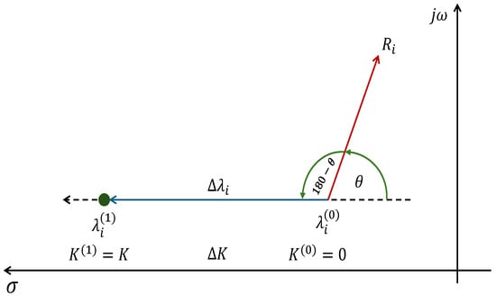
Figure 1. Schematic phase compensation by residue.

From (8), it follows that the residue $R_{ji}$ quantifies the sensitivity of the eigenvalue associated with the state matrix $\mathbf{A}$ to specific input–output channels. This information is valuable for identifying which inputs are most effective for control action and feedback, thereby guiding the design and placement of stabilizing devices. In commercial power system analysis tools, such as DIgSILENT PowerFactory, the state matrix $\mathbf{A}$, its eigenvalues, and the corresponding eigenvectors are typically available; however, the input and output matrices $\mathbf{B}$ and $\mathbf{C}$ are not directly accessible.

To overcome this limitation, ref. [17] proposed a methodology for constructing the matrices $\mathbf{B}$ and $\mathbf{C}$ within the DPL environment. By reconstructing these matrices, it becomes possible to compute residues directly from the available modal information, enabling the evaluation of system controllability from relevant inputs such as generators equipped with PSS devices.

To construct the matrices $\mathbf{B}$ and $\mathbf{C}$, the first step is to extract the state matrix $\mathbf{A}$ from the modal analysis results. Unlike $\mathbf{A}$, which is unique for a given operating point, the matrices $\mathbf{B}$ and $\mathbf{C}$ depend on the choice of system inputs and outputs.

In the second step, the columns of $\mathbf{B}$ are determined by evaluating the variation of the state vector $\mathbf{x}\left(t\right)$ in response to perturbations in selected inputs. Specifically, the i-th column ${\mathbf{b}}_i$ of $\mathbf{B}$ can be obtained by applying a perturbation in active power injection at bus i. The perturbed system dynamics can be expressed as [27]

$$\mathrm{\Delta }\dot{\mathbf{x}}\left(t\right)=\mathbf{A}\mathrm{\Delta }\mathbf{x}\left(t\right)+{\mathbf{b}}_i\mathrm{\Delta }{u}_i\left(t\right),$$

(12)

where $\mathrm{\Delta }\mathbf{x}\left(t\right)$ is the deviation in state variables and $\mathrm{\Delta }{u}_i\left(t\right)$ is the perturbation at the i-th input channel.

Assuming a unit-step input $\mathrm{\Delta }{u}_i\left(t\right)$ applied at $t=0$ with $\mathrm{\Delta }\mathbf{x}\left(t\right)=\mathbf{0}$ for $t\le 0$, the solution of (12) using Euler’s forward approximation is obtained as

$${\mathbf{b}}_i\approx \mathrm{\Delta }\dot{\mathbf{x}}\left(\mathrm{\Delta }t\right)\approx {\displaystyle \frac{\mathrm{\Delta }\mathbf{x}\left(\mathrm{\Delta }t\right)-\mathrm{\Delta }\mathbf{x}\left(0\right)}{\mathrm{\Delta }t}}={\displaystyle \frac{\mathbf{x}\left(\mathrm{\Delta }t\right)-\mathbf{x}\left(0\right)}{\mathrm{\Delta }t}}.$$

(13)

Since $\mathrm{\Delta }\mathbf{x}\left(0\right)=\mathbf{0}$ and $\mathrm{\Delta }{u}_i\left(t\right)=1$, a sufficiently small time step (e.g., $\mathrm{\Delta }t={10}^{-4}$ s) ensures that the approximation error is negligible. This step size was selected through a trial-and-error comparison between the responses of the full nonlinear model and its linearized counterpart.

In the third step, the output matrix $\mathbf{C}$ is constructed according to the selected system outputs. Each row corresponds to a monitored generator, with zeros in all positions except for a single entry equal to one in the column associated with the generator’s output variable (e.g., rotor speed). This formulation enables the mapping of the full state vector $\mathbf{x}\left(t\right)$ to the measured outputs $\mathbf{y}\left(t\right)$.

Once $\mathbf{B}$ and $\mathbf{C}$ are obtained, and the left and right eigenvectors associated with the critical mode are identified, the corresponding residues can be computed accurately, thereby allowing the assessment of controllability and observability of oscillatory modes from relevant inputs such as generators equipped with PSS devices.

3. Automated Residue Computation for Modal Analysis in PowerFactory

This section presents the proposed methodology for computing residues from the modal analysis results of a power system model implemented in DIgSILENT PowerFactory.

As discussed in the previous section, the computation of residues requires access to the state matrix $\mathbf{A}$ together with the associated eigenvalues, left eigenvectors, and right eigenvectors. Although DIgSILENT PowerFactory does not directly provide residue calculations, it offers all the necessary components to implement them through its scripting environment. The developed procedure leverages PowerFactory’s internal data export and modal analysis capabilities, as illustrated in Figure 2.

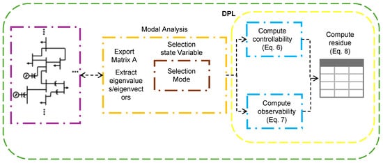
Figure 2. Flow chart for residue calculation.

The process begins by extracting the state matrix $\mathbf{A}$ from the small-signal model using PowerFactory’s Modal Analysis tool. The matrix is exported in .mtl format, accompanied by an index file (VariableToIdx_Amat.txt) that maps each state variable to its matrix position. Simultaneously, the eigenvalues and eigenvectors are retrieved from the modal analysis module. These quantities constitute the mathematical foundation for modal controllability, observability, and residue evaluation.

A dedicated DPL (DIgSILENT Programming Language) script automates the subsequent steps, as outlined in the flowchart. First, the script selects the desired oscillation mode and corresponding state variables. It then computes the controllability coefficients $B_{kp}^{\prime }$ and observability coefficients $C_{qk}^{\prime }$. Finally, residues $R_{qpk}=C_{qk}^{\prime }{B}_{kp}^{\prime }$ are computed for each input–output pair and stored in a structured data table for post-processing. This implementation avoids external data manipulation, providing an integrated, repeatable, and scalable residue analysis workflow directly within PowerFactory.

Figure 2 summarizes the overall algorithm: from matrix and eigenvector extraction, through DPL-based computation of controllability and observability, to automated residue assembly. The process serves as a foundation for residue-guided controller tuning, enabling systematic analysis of mode controllability and damping effectiveness within the same simulation environment.

Building on these capabilities, a custom script was developed in the DPL to automate residue computation.

To perform modal analysis and extract the required data, the PowerFactory objects ComMod* and ComInc* must be configured. These objects manage the export of state-space matrices (such as $\mathbf{A}$), eigenvalues, and eigenvectors to a user-defined script (Algorithm 1). The algorithm initializes the study case by opening the project folder, retrieving cases, and activating the selected one. Next, ComInc computes the initial operating point, while ComMod is set to run the modal analysis. Export flags are then defined; for example, Modal.iSysMatMat=1 exports $\mathbf{A}$, Modal.iEvMat=1 and Modal.iREVMat=1 export right and left eigenvectors, and Modal.dirMat=path specifies the output directory. Finally, Initial.Execute() and Modal.Execute() are called to obtain the numerical data needed for residue computation.

PowerFactory uses a color-coded syntax in DPL: black for user-defined variables, green for comments, red for user input text and commands, and blue for internal DPL functions. Each instruction must be terminated with a semicolon (;) to ensure proper execution.

Algorithm 1 DPL script for modal analysis and selection of output matrices

1: ! Section defined type variables   2: string path;   3: set StudyCases;   4: object Folder,Case,Initial,Modal;   5: ! Section defined study case of grid   6: Folder = GetProjectFolder(study);   7: StudyCases = Folder.GetContents(*.IntCase);   8: StudyCases.SortToName(0);   9: Case = StudyCases.First(); 10: Case.ShowFullName(); 11: Case.Activate(); 12: Case.ShowFullName(); 13: ! Defined object by 14: Initial = GetCaseCommand(ComInc);      ▹ !calculation initial conditions 15: Modal = GetCaseCommand(ComMod);        ▹ !modal analysis 16: path =’D:\Taller Small-Signal\Clase Residuo’; 17: ! Section by vector and matrix of modal analysis 18: Modal:iLeft = 0; 19: Modal:iRight = 0; 20: Modal:iPart = 0; 21: Modal:iSysMatMat = 1; 22: Modal:iEvMat = 1; 23: Modal:iREVMat = 1; 24: Modal:iEVMat = 1; 25: Modal:iPartMat = 0; 26: Modal:dirMat = path; 27: ! Execution of simulation of modal analysis 28: Initial.Execute(); 29: Modal.Execute();

Once the modal analysis data has been exported, the input matrix $\mathbf{B}$ is built by simulating active power injections at selected buses. The target bus is specified with the general selection command SetSelect*. The i-th column of $\mathbf{B}$ is obtained by applying a unit step in active power—modeled as a 100 MW load increase—at the corresponding bus, as defined in (13). This perturbation is introduced through a manually created EvtSwitch* event linked to a mobile load connected to the selected terminal element (ElmTerm*). After linking the load, the initial conditions (ComInc*) and the dynamic simulation (ComSim*) are executed to capture the system response. By superposition, the full matrix $\mathbf{B}$ is assembled by repeating this procedure for each bus in the system.

Algorithm 2 shows the implementation of this process in DPL. The first section declares the required variables and initializes objects such as study cases, events, and results containers. Then, the script imports the mapping file VariableToIdx_Amat.txt, which links state variables to the indices of matrix $\mathbf{A}$, and configures simulation parameters. Next, the Algorithm defines the switching event used to apply the power perturbation and retrieves the network terminals (ElmTerm*) that serve as candidate buses. In the construction phase, the script iteratively reads variable indices, extracts simulation results, and computes incremental changes in the state vector caused by the perturbation. Finally, these increments are normalized with respect to the applied step and stored as entries of $\mathbf{B}$ through the MatrixB.Set command. This procedure guarantees that each column of $\mathbf{B}$ accurately represents the controllability of the system with respect to active power injections at the corresponding bus.

For large-scale systems, the construction of matrix $\mathbf{B}$ through per-input perturbations should be restricted to a filtered subset of candidate actuators. In such cases, normalization of the resulting controllability and observability terms is recommended to enhance numerical robustness across states and operating points.

To ensure dimensional consistency between the simulated perturbations and the linearized state-space formulation in (1), each column of the input matrix $\mathbf{B}$ was explicitly normalized by the amplitude of the applied active-power step. The formulation adopted is

$$B_i={\displaystyle \frac{\mathrm{\Delta }x}{\mathrm{\Delta }P}},$$

where $\mathrm{\Delta }x$ represents the incremental state deviation and $\mathrm{\Delta }P=100\mathrm{MW}$ corresponds to the temporary active-power increase applied at the selected bus. This normalization guarantees that $\mathbf{B}$ preserves the correct physical units and remains compatible with the state-space model $\dot{x}=Ax+Bu$.

The 100 MW perturbation was chosen as a practical compromise between ensuring numerical observability and maintaining operation within the linear region around the steady-state point. Across all buses tested in the benchmark systems, the induced rotor-angle deviations remained below $0.2^{°}$, and rotor-speed deviations were less than $1\times {10}^{-4}$ p.u., confirming that the system response lies firmly within the small-signal regime. Consequently, the linearization underlying the modal formulation remains valid, and the computed $\mathbf{B}$ entries faithfully represent the system’s controllability coefficients.

To validate the linearity assumption, a sensitivity analysis was performed using smaller perturbations of 10 MW and 20 MW. The resulting columns of $\mathbf{B}$ exhibited nearly proportional scaling with the applied step magnitude, with deviations below 1% across all tested buses. The corresponding eigenvalues showed frequency variations smaller than 0.01 Hz and damping-ratio deviations below 0.001%, confirming that the system dynamics scale linearly within this range.

These results demonstrate that the 100 MW perturbation is sufficiently small to preserve linearity, yet large enough to overcome numerical precision limits within the DPL environment. Therefore, the resulting input matrix $\mathbf{B}$ is dimensionally consistent, numerically stable, and representative of the system’s controllability characteristics under small disturbances.

Algorithm 2 DPL Script for Matrix B Construction

1: ! Section defined type variables   2: string path,str,input description,s,file1;   3: set terms,events;   4: object event,term,node,switch,Results,inicial,sim,inputs,MatrixB;   5: ! Selection elements   6: file1 = ‘VariableToIdx_Amat.txt’;   7: s = sprintf(‘%s\\%s’,path,file1);   8: inicial = GetCaseCommand(‘ComInc’);   9: sim = GetCaseCommand(‘ComSim’); 10: MatrixB = GetCaseObject(‘MatrixB.IntMat’); 11: MatrixB.Init(1,1); 12: ! Calculations 13: inicial:p resvar = Results; 14: inicial:dtgrd = 0.0001; 15: inicial:tstart = 0; 16: inicial:dtout = 0.0001; 17: sim:stop = 0.0001; 18: events = inputs.GetContents(); 19: event = events.First(); 20: event:time = 0; 21: event:i switch = 1; 22: terms = SEL.GetAll(’ElmTerm’); 23: terms.SortToName(0); 24: term = terms.First(); 25: ! Construction matrix B 26: MatrixB = GetCaseObject(’MatrixB.IntMat’); 27: fopen (s,‘r’,0); 28: while (ierr > −1) { 29:      if(count = 1){ 30:         ierr = fscanf(0,‘%d’,index); 31:         count = count + 1 ;} 32: if (count > 1) { 33:      while(count > 1.and.count < 4.and.ierr > −1) { 34:         ierr = fscanfsep(0,‘%s’,path,”,0); 35:         if (count < 3) { 36:             count = count + 1; 37:             i1 = strstr(path,‘Grid Name’); 38:             str1 = strcpy(path,i1,120); 39:             i2 = strstr(str1,‘ ’); 40:             str2 = strcpy(str1,0,i2); 41:             Filter.objset = str2; 42:             elements = Filter.Get(); 43:             element = elements.First(); 44:         } 45:         else { 46:             count = 1; 47:             var = sprintf(s,‘%s’,path); 48:             col = ResIndex(Results,element,var); 49:             GetResData(aux_ini,Results,row,col); 50:             GetResData(aux end,Results,nval-1,col); 51:             aux = (aux end-aux ini)/txx; 52:             MatrixB.Set(index,column,aux); 53:             Results.Flush(); }}}} 54: fclose(0);

The integration time step was fixed at $\mathrm{\Delta }t=1\times {10}^{-4}$ s with a total simulation horizon of 0.1 ms. This setting was selected after convergence tests in which decreasing $\mathrm{\Delta }t$ by one order of magnitude produced eigenvalue and damping-ratio variations below 0.05%.

The chosen step size therefore provides sufficient numerical resolution for all generator buses and operating points while avoiding unnecessary computational cost.

Because the modal residue computation relies on the linearized Jacobian matrices exported by ComMod, the integration step primarily affects transient verification runs and not the modal results themselves. Across all test cases, no stiffness-related divergence or integration failure was observed.

For the output matrix $\mathbf{C}$, the system considers the rotor speed of all synchronous machines as the primary output variables, since PSSs are implemented within the generator excitation systems. Each row of $\mathbf{C}$ corresponds to a generator and contains only zeros, except for a single entry with value “1” at the position associated with the generator’s speed state. This assignment is illustrated in Algorithm 3.

In Algorithm 3, the script reads the file VariableToIdx_Amat.txt, which maps state variables to their indices, and scans each entry until it identifies those labeled as speed. When such a variable is found, the index is stored in the auxiliary matrix Cindex, and the association between generator and state variable is reported through the fprintf command. Once all relevant variables are identified, the script initializes the output matrix $\mathbf{C}$ with the appropriate dimensions, and each speed state is assigned a unit entry in the corresponding row, while the rest of the elements remain zero. This procedure ensures that $\mathbf{C}$ correctly maps the system states to measurable outputs, enabling the analysis of modal observability from generator speeds. Nevertheless, other output variables may be selected depending on the specific application or analysis requirements.

The same procedure applies to non-generator actuators (FACTS/HVDC/IBR): construct matrix B from the device’s control inputs and define matrix $\mathbf{C}$ with measurements aligned to the targeted oscillation that permit computation for residue.

In DIgSILENT PowerFactory, modal module (ComMod) exports the state-to-index map in the text file VariableToIdx_Amat.txt. In our implementation, the output vector y selects rotor speed for each synchronous generator by matching the literal state label speed in that file. During execution, it records the full object name of each machine and exact speed state index used to place the unit entry in C. Example of Kundur system: G1.speed, G2.speed, G3.speed, G4.speed. This guarantees that any user can reconstruct our row selectors directly from PowerFactory users’ exported names without ambiguity.

The residue is then computed following the relationships defined in (6)–(8), with Algorithm 4 implementing these operations explicitly. First, the script reads the file EVals.mtl, which contains the system eigenvalues, and calculates their damping ratios, storing them in MEdamp. Modes with insufficient damping (e.g., $\left|\zeta \right|<0.1$) are identified and indexed in Mindx as critical modes of interest. For each selected mode, the corresponding left and right eigenvectors are retrieved from the files lEV.mtl and rEV.mtl, respectively, and their real and imaginary components are stored in Mreal and Mimag.

With the input matrix $\mathbf{B}$ and the output matrix $\mathbf{C}$ already constructed as described in Section 2, the script proceeds to evaluate modal controllability and observability by multiplying the eigenvectors with the appropriate columns of $\mathbf{B}$ and rows of $\mathbf{C}$. These calculations directly implement the definitions in (6) and (7), with the magnitude and angle of each term stored in Mctrl_m/Mctrl_ang and Mobser_m/Mobser_ang, respectively. Finally, the residue for each mode and input–output pair is obtained by combining the controllability and observability results according to (8), with the residue magnitude recorded in MResidue_m and its phase in MResidue_ang. This systematic procedure not only ensures a consistent link between modal theory and practical implementation in PowerFactory, but also provides the necessary data for residue-based analysis and controller tuning in power system stability studies.

Algorithm 3 DPL Script for Matrix C Construction

1: ! Section defined type variables   2: string var,str1,str2,output description,s,file1,s2,file2;   3: set elements;   4: object element,Cindex,MatrixC;   5: int ierr,count,i1,i2,comp,a,m,row,col;   6: double index,aux;   7: ! Selection elements   8: ier = −1;   9: count = 1; 10: aux = 1; 11: file1 = ‘VariableToIdx_Amat.txt’; 12: s = sprintf(‘%s\\%s’,path,file1); 13: Cindex = GetCaseCommand(‘Cindex.IntMat’); 14: Cindex.Init(1,1); 15: ! Construction matrix C 16: fopen(s,‘r’,0); 17: while (ierr > −1) { 18:      if(count = 1){ 19:         ierr = fscanf(‘0,%d’,index); 20:         count = count + 1;} 21: if(count > 1) { 22:      while(count > 1.and.count < 4.and.ier > −1) { 23:         ier = fscanfsep(0,‘%s’,path,“”,0); 24:         if(count < 3) { 25:             count = count + 1; 26:             i1 = strstr(path,‘Grid Name’); 27:             str1 = strcpy(Dpath,i1,120); 28:             i2 = strstr(str1,‘ ’); 29:             str2 = strcpy(str1,0,i2); 30:         } 31:         else { 32:             comp = strcmp(path,‘speed’); 33:             if(comp = 0){ 34:                Cindex.Set(aux,1,index); 35:                fprintf(1,‘Output %d is state variable number %d from%s’,aux,index,str2); 36:                aux = aux + 1;}}}}} 37: fclose(0); 38: MatrixC = GetCaseCommand(‘MatrixC.IntMat’); 39: row = Cindex.NRow(); 40: col = index − 2; 41: MatrixC.Init(row,col); 42: for(m = 1; m <= row + 1; m = m + 1){ 43:      a = Cindex.Get(m,1); 44:      MatrixC.Set(m,a,1); 45:     }

Algorithm 4 DPL Script for Residue Calculation (Part I)

1: ! Section defined type variables   2: double b, real, imag, damp, ar, ai, sumr, sumi, ctl_m, ctl_ang, obser_m, obser_ang,res_m, double res_ang;   3: int h, error, mode, x, y, colum, row, count, ierr, n, nE, nI, nL, nb, nC, col, rowI, rin;   4: object B, C, Mindex, MEdamp, Mreal, Mimag, Mctrl_m, Mctrl_ang, Mobser_m, Mobser_ang, MResidue_m, MResidue_ang;   5: ! Selection elements   6: file1 = ‘EVals.mtl’; file2 = ‘lEV.mtl’; file3=‘rEV.mtl’; EVals = sprintf(‘%s\\%s’,path,file1); 1EV = sprintf(‘%s\\%s’,path,file2); rEV = sprintf(‘%s\\%s’,path,file3);   7: B = GetCaseCommand(‘MatrixB.IntMat’);   8: C = GetCaseCommand(‘Cindex.IntMat’);   9: Mindx = GetCaseCommand(‘Mindx.IntMat’); 10: MEdamp = GetCaseCommand(‘MEdamp.IntMat’); 11: Mreal = GetCaseCommand(‘Mreal.IntMat’); 12: Mimag = GetCaseCommand(‘Mimag.IntMat’); 13: Mctrl_m = GetCaseCommand(‘Mctrl_m.IntMat’); 14: Mctrl_ang = GetCaseCommand(‘Mctrl_ang.IntMat’); 15: Mobser_m = GetCaseCommand(‘Mobser_m.IntMat’); 16: Mobser_ang = GetCaseCommand(‘Mobser_ang.IntMat’); 17: MResidue_m = GetCaseCommand(‘MResidue_m.IntMat’); 18: MResidue_ang = GetCaseCommand(‘MResidue_ang.IntMat’); 19: ! Selection respective eigenvalue 20: fopen(EVals,‘r’,0); 21: while(ierr > −1) { 22:      if (colum = 1){ierr = fscanf(0,‘%d’,x); colum = 2; } 23:      if (colum = 2){ierr = fscanf(0,‘%d’,y); colum = 3;} 24:      if (colum = 3){ierr = fscanf(0,‘%d’,real); colum = 4;} 25:      if (colum = 4){ierr = fscanf(0,‘%d’,imag); colum = 1;} 26:      if (ierr > −1) { damp=real/sqrt(real*real+imag*imag); 27:                    MEdamp.Set(n,1,damp); n = n + 1;}} 28: fclose(0); 29: nE = MEdamp.NRow(); n = 1; 30: for (row=1; row < (nE + 1); row = row + 1){ 31:      damp = MEdamp.Get(row,1); 32:      if (abs(damp) > 0 .and. abs(damp) < 0.1){ 33:         Mindx.Set(n,1,row); n = n + 1;}} 34: ! Controllability 35: nI = Mindx.NRow(); 36: for (rowI = 1; rowI < (nI + 1); rowI = rowI + 1){ 37:      mode = Mindx.Get(rowI,1); 38:      fopen(IEV,‘r’,0); count = 1; ierr = 1; 39:      while (ierr > −1){ 40:         if (count = 1) {ierr = fscanf(0,‘%d’,x); count = 2;} 41:         if (count = 2) {ierr = fscanf(0,‘%d’,y); count = 3;} 42:         if (count = 3) {ierr = fscanf(0,‘%d’,real); count = 4;} 43:         if (count = 4) {ierr = fscanf(0,‘%d’,imag); count = 1;} 44:         if (y = mode) {Mreal.Set(1,x,real); Mimag.Set(1,x,imag);}} 45: fclose(0); 46: nL = Mreal.NCol();    nb = B.NCol(); 47: for (col = 1; col < (nb+1); col = col + 1){ 48:      sumr = 0;      sumi = 0; 49:      for (row = 1; row < (nL + 1); row = row + 1){ 50:         ar = Mreal.Get(1,row);      ai = Mimag.Get(1,row);      b = B.Get(row,col); 51:         sumr = sumr + ar*b;      sumi = sumi + ai*b;} 52:      ctrl_m = sqrt(sumr*sumr+sumi*sumi);      ctrl_ang = atan2(sumi/sumr); 53:      Mctrl_m.Set(rowI,col,ctrl_m);      Mctrl_ang.Set(rowI,col,ctrl_ang);}

Algorithm 4 DPL Script for Residue Calculation (Part II)

1: ! Observability   2: ! .......... Similar to controllability   3: ! Construction of Residue   4: nI = Mobser_m.NRow();   5: nC = Mobser_m.NCol();   6: for (row = 1; row < (nI + 1); row = row + 1){   7:      for (col = 1; col < (nc + 1); col = col + 1){   8:         ar = Mobser_m.Get(row,col);   9:         ai = Mctrl_m.Get(row,col); 10:         res_m = ar*ai; 11:         MResidue_m.Set(row,col,res_m); 12:         ar = Mobser_ang.Get(row,col); 13:         ai = Mctrl_ang.Get(row,col); 14:         res_ang = ar+ai; 15:         MResidue_ang.Set(row,col,res_ang);}}

4. Simulation Results and Case Studies

To assess the generalizability and robustness of the proposed methodology, this section presents two case studies that are widely referenced in the specialized literature. The first is a benchmark academic system for small-signal stability analysis, characterized by its low-controllability oscillation modes. The second is a reduced model of the New York–New England power grid, frequently employed as a standard test system for evaluating damping strategies in multi-area networks. This latter system contains numerous buses and several lightly damped oscillatory modes, thus providing a challenging environment for validating the effectiveness of the proposed residue-based approach.

All simulations were conducted using DIgSILENT PowerFactory 2024 SP2 on a 64-bit Windows 11 platform. The file pfd and data for one of test systems can be obtained from the following public repository: https://github.com/joscullo/My-Powerfactory/tree/main (accessed on 13 October 2025).

4.1. Academic Benchmark System

Figure 3 shows the single-line diagram of the test system used in this study, widely known as the Two-Area Kundur Test System. This benchmark model, first introduced in [1] (Example 12.6), has become a classical reference in small-signal stability analysis. It represents two interconnected areas linked by a weak tie-line, with each area comprising two synchronous generators [1,10,15]. Due to its representative structure and dynamic characteristics, this system has been extensively adopted in a wide range of studies as a standard testbed for validating methodologies in oscillation analysis, stability assessment, and controller design.

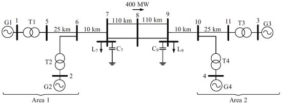
Figure 3. Single-line diagram of two-area test system [1].

Table 1 summarizes the dominant oscillatory modes of the Two-Area Kundur System in the absence of supplementary damping controllers such as PSSs. The eigenvalue analysis reveals at least three poorly damped modes, each associated with a complex-conjugate pair, exhibiting damping ratios well below the 10% stability requirement typically imposed by grid codes. In particular, Mode 3, with a damping ratio of only 0.12%, corresponds to an inter-area oscillation in the 0.5 Hz range, which is a critical frequency band for large interconnected systems. Modes 13 and 15, on the other hand, are local oscillations close to 1 Hz, also falling below the recommended damping threshold.

Table 1. Dominant oscillatory modes of the Two-Area Kundur Test System without PSS controllers.

Mode	Real [1/s]	Imaginary [rad/s]	Angle [deg]	Damping Frequency [Hz]	Damping Ratio [%]
3	−0.0352	3.052	89.93	0.486	0.12
13	−0.4600	6.225	85.77	0.990	7.37
15	−0.4870	6.419	85.66	1.021	7.57

These results emphasize the necessity of introducing damping controllers, specifically PSSs, in order to improve the system’s small-signal stability. The placement and tuning of such devices can be effectively guided by the residue-based methodology presented in this paper. As described in Section 2, residues provide a direct measure of modal controllability and observability by combining the left and right eigenvectors with the input and output matrices $\mathbf{B}$ and $\mathbf{C}$. The codes implemented in DPL (Algorithms 1–4) automate this process, enabling the identification of the generators with the highest residues for each oscillatory mode. This contribution bridges the gap between modal theory and practical implementation in PowerFactory, offering a systematic framework for controller allocation and tuning in realistic system studies.

Figure 4 shows the eigenvalue spectrum of the Two-Area Kundur Test System plotted in the complex plane, obtained through the modal analysis module in DIgSILENT PowerFactory. The distribution of eigenvalues clearly distinguishes between local and inter-area oscillatory dynamics. Most eigenvalues are clustered around frequencies above 1 Hz, corresponding to local generator oscillations with acceptable damping ratios. In contrast, one inter-area mode (mode 3), located near the imaginary axis at approximately 0.5 Hz, exhibits an extremely low damping ratio of $\zeta =0.12\%$. This small negative real part indicates that even minor disturbances can trigger sustained oscillations of significant amplitude, thereby posing a risk to system stability.

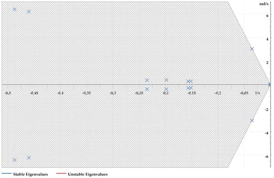
Figure 4. Complex plane of eigenvalues.

The identification of such poorly damped modes provides the basis for the residue-based analysis developed in this work. By combining the eigenvalue information with the controllability and observability indices derived from the $\mathbf{B}$ and $\mathbf{C}$ matrices (see (6)–(8)), the proposed codes implemented in DPL can automatically determine which generators offer the highest residues for each oscillation mode. This enables a systematic and technically grounded selection of candidate locations for PSSs, ensuring that damping is improved precisely where the system dynamics are most sensitive. Hence, the results in Figure 4 not only reveal the presence of critical oscillatory behavior but also motivate the application of the automated residue-computation framework presented in this paper.

Figure 5 presents the residue distribution and corresponding participation factors for mode 13, as obtained from the modal analysis in PowerFactory. Although residues are computed for all system elements, only a subset of generators exhibit significant values, highlighting their dominant influence on the selected oscillatory mode. In particular, $G_1$ and $G_2$ show the largest residue magnitudes, consistently aligned with the highest participation factors. This result confirms that these machines provide the most effective controllability and observability for mode 13, making them the primary candidates for the allocation of damping controllers such as PSSs. The smaller, yet nonzero, residue values observed in $G_3$ and $G_4$ indicate that these generators still participate in the mode dynamics, albeit to a limited extent. Such information is relevant when considering coordinated or distributed damping strategies, where secondary controllers can complement the action of primary PSSs.

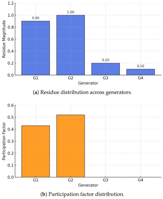
Figure 5. Residue and participation factor of mode 13.

Table 2 extends this analysis by comparing the residue magnitudes and angles across three critical modes: the inter-area mode 3 and the local modes 13 and 15. For the inter-area mode 3, residues are relatively small for all generators, reflecting the difficulty of damping this type of oscillation. By contrast, in mode 15 the residues of $G_3$ and $G_4$ are significantly larger than those of $G_1$ and $G_2$, indicating that the controllability of this local oscillation shifts towards the machines located in Area 2. This complementary behavior across modes emphasizes the importance of a residue-based allocation strategy; while $G_1$ and $G_2$ are the natural candidates for damping the inter-area and mode 13 oscillations, $G_3$ and $G_4$ become essential when addressing local oscillations associated with mode 15.

Table 2. Residue of Example Kundur.

Gen	Mode 3		Mode 13		Mode 15
	Residue	Angle (°)	Residue	Angle (°)	Residue	Angle (°)
1	2.04 × 10−3	88.99	9.24 × 10−3	−85.63	8.98 × 10−3	−84.59
2	1.56 × 10−3	89.89	10.63 × 10−3	−85.90	8.89 × 10−3	−80.72
3	7.68 × 10−3	−88.89	1.99 × 10−3	−80.15	1.69 × 10−2	−85.71
4	6.88 × 10−3	−88.98	1.41 × 10−3	−77.61	2.14 × 10−2	−86.13

Overall, the combined results from Figure 5 and Table 2 demonstrate the ability of the proposed residue-based framework to identify, in a systematic manner, which generators contribute most to the controllability and observability of each oscillatory mode. This capability provides a strong technical justification for targeted PSS placement, ensuring that damping resources are deployed where they are most effective for enhancing small-signal stability.

Using (10), the displacement of the critical eigenvalues can be estimated to determine the controller gains required to achieve a target damping ratio of at least 10%. Figure 6 illustrates this behavior in the complex plane, where the open-loop eigenvalues of the system (blue circles) are shifted leftwards (black markers) as the residue-based tuning procedure is applied. The dashed lines indicate constant damping-ratio loci (3%, 7%, and 10%), which serve as reference boundaries for evaluating the effectiveness of the applied control action. The figure highlights that, prior to compensation, the inter-area mode lies very close to the imaginary axis, with a damping ratio below 1%, confirming the critical nature of this oscillation as discussed in Figure 4 and Table 1. After residue-guided tuning, the eigenvalue trajectory crosses the 10% damping locus, thereby fulfilling the stability requirement commonly adopted in power system operation, as shown in Table 3. This result validates the use of residues as sensitivity measures that directly relate controller action to eigenvalue displacement.

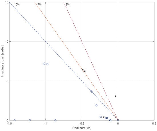
Figure 6. Displacement of eigenvalues through residue procedure.

Table 3. Dominant oscillatory modes of the Two-Area Kundur Test System with PSS controllers.

Mode	Real	Imaginary	Angle	Damping Frequency	Damping Ratio
	[1/s]	[rad/s]	[deg]	[Hz]	[%]
3	−0.3152	3.122	84.23	0.497	10.04
13	−0.9810	7.125	82.14	1.130	13.67
15	−1.0570	7.159	81.65	1.138	14.53

By combining the residue information shown in Figure 5 and Table 2, which identify $G_1$ and $G_2$ as the most effective locations for damping control, the procedure demonstrated in Figure 6 provides a systematic and technically justified methodology for both the allocation and tuning of PSSs. Hence, the proposed framework not only identifies where controllers should be placed, but also quantifies the expected improvement in damping, bridging the gap between modal theory and practical implementation in PowerFactory.

4.2. New York–New England Power Grid

Figure 7 depicts the single-line diagram of the reduced New York–New England (NY–NE) power system, a widely used benchmark in small-signal stability studies [1]. The model consists of 66 buses, 16 synchronous generators, 28 transformers, and 52 transmission lines, grouped into three interconnected regions (Areas A, B, and C). Transmission voltage levels include 380 kV, 220 kV, 110 kV, and 15.75 kV, as indicated in the diagram. This system is particularly attractive for modal analysis because it captures both local oscillations, typically associated with interactions between nearby machines, and inter-area oscillations, which arise from power exchanges between distant areas through weak tie-lines. Such dynamic characteristics make the NY–NE system a more complex and realistic test case compared to the two-area Kundur model, providing a rigorous platform for validating the proposed residue-based framework in scenarios with higher system dimensionality, stronger coupling, and multiple oscillatory modes.

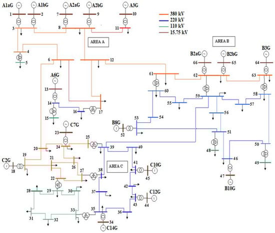
Figure 7. Diagram of reduced Power System of New York–New England [1].

Consistent with the findings from the Kundur system, the reduced New York–New England network also exhibits critical oscillatory dynamics. As shown in Table 3, three dominant modes are identified, among which mode 114 is particularly concerning, since its eigenvalue presents a positive real part and therefore corresponds to an unstable inter-area oscillation. Modes 106 and 112, while stable, display relatively low damping ratios (6.77% and 4.56%, respectively), falling close to or below the commonly accepted 10% threshold. These results highlight the vulnerability of large-scale interconnected systems to both poorly damped and unstable modes, reinforcing the need for systematic damping strategies.

Table 4 complements this analysis by reporting the residues associated with each generator for the critical modes. The residue magnitudes reveal that not all machines contribute equally to modal controllability and observability. For example, B10G and A1bG exhibit the highest residues in modes 106 and 114, while C7G shows strong influence in mode 112. This distribution of modal sensitivities provides valuable insight into the optimal placement of PSSs, as it identifies the generators where control action can most effectively shift eigenvalues towards the stable region.

Table 4. Residue of New York–New England.

Gen	Mode 106		Mode 112		Mode 114
	Residue	Angle (°)	Residue	Angle (°)	Residue	Angle (°)
A1aG	0.1298	−96.15	0.5769	−68.39	0.6914	108.31
A1bG	0.6979	−7.18	0.5140	−64.27	0.8576	108.30
A2aG	0.0129	−105.23	0.4950	−148.39	0.5736	125.12
A2bG	0.1336	−99.36	0.6179	−68.46	0.6066	107.72
A3G	0.1096	−99.66	0.4933	−67.25	0.5933	109.78
B10G	0.1759	−104.76	0.8367	−69.32	1.0000	106.30
B2aG	0.0008	37.69	0.5229	−58.72	0.3369	102.83
B2bG	0.0005	−131.17	0.0194	−127.72	0.0067	33.32
B3G	0.0023	−1.41	0.0110	−120.44	0.0291	41.18
C0G	0.0018	−144.01	0.0218	−113.46	0.0127	−121.57
C10G	0.0001	−137.97	0.0212	−115.83	0.0115	36.25
C12G	0.0099	1.17	0.3336	70.05	0.0339	−123.25
C14G	0.0176	−5.32	0.0730	−115.39	0.0121	−121.27
C2G	0.0023	1.42	0.1204	72.32	0.0206	−120.37
C7G	0.1000	−66.70	1.0000	−156.41	0.6283	64.74

When the proposed residue-based tuning methodology is applied, PSS parameters are adjusted at the most influential generators, as determined by their residue values. This process ensures that controller effort is concentrated where it yields the maximum damping improvement. The effect of this tuning is illustrated in Figure 8, which shows the displacement of oscillatory modes in the complex plane. Open-loop eigenvalues are depicted as blue circles, while the closed-loop eigenvalues—after the installation and tuning of PSSs at the identified generators—are represented by black markers. The dashed lines correspond to constant damping-ratio loci (3%, 7%, and 10%), serving as reference boundaries for evaluating system performance, as shown in Table 5.

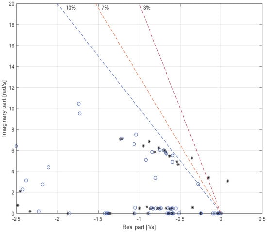
Figure 8. Displacement of oscillatory modes through residue.

Table 5. Dominant oscillatory modes of the New England Test System with PSS controllers.

Mode	Real	Imaginary	Angle	Damping Frequency	Damping Ratio
	[1/s]	[rad/s]	[deg]	[Hz]	[%]
114	−0.2750	2.722	84.23	0.433	10.06
112	−0.8710	3.525	76.12	0.560	23.98
106	−0.9270	5.263	80.08	0.838	17.22

The figure highlights that several modes originally located near the imaginary axis, including the unstable inter-area mode 114, are effectively shifted leftwards beyond the 10% damping locus. This confirms that the residue-based tuning not only suppresses instability but also significantly enhances the damping of poorly damped oscillations. Moreover, the dispersion of eigenvalues across a wide frequency range demonstrates the scalability of the approach in handling both local and inter-area dynamics in a large-scale system. The coordinated displacement of multiple eigenvalues further validates the residue framework as a systematic tool for simultaneously improving the damping of critical modes, ensuring that stability margins are achieved across the entire network.

Overall, the results from Table 5 and Table 6, together with the eigenvalue displacements shown in Figure 8, demonstrate the scalability and robustness of the proposed framework. By systematically combining eigenvalue analysis with residue-based sensitivity information, the methodology provides a principled approach for both the allocation and tuning of damping controllers in complex, realistic systems such as the NY–NE network. This directly validates the contribution of our work, bridging theoretical modal indices with automated practical implementation in Power Factory.

Table 6. Dominant oscillatory modes of the New England Test System without PSS controllers.

Mode	Real	Imaginary	Angle	Damping Frequency	Damping Ratio
	[1/s]	[rad/s]	[deg]	[Hz]	[%]
114	0.079	3.081	88.52	0.490	−2.59
112	−0.155	3.388	87.38	0.539	4.56
106	−0.357	5.257	86.12	0.837	6.77

For this case Table 7 shows, for illustrative purposes, the PSS parameters of generators $B10G$, $A1bG$ and $C7G$ using residue according to criteria in reference [25], which is beyond the scope of this paper.

Table 7. PSS parameter controllers of New England test system.

Gen	Tw (s)	Gain	${\mathit{T}}_1$ (s)	${\mathit{T}}_2$ (s)	${\mathit{T}}_3$ (s)	${\mathit{T}}_4$ (s)
B10G	10	119.5	0.385	0.108	0.421	0.089
A1bG	9.5	96.1	0.462	0.093	0.448	0.090
C7G	9.8	149.7	0.171	0.039	0.498	0.100

4.3. Method Verification and Robustness Analysis

The accuracy of the proposed automated residue computation was verified through multiple validation steps. First, residues obtained from the developed DPL scripts were compared against the participation factors computed by DIgSILENT PowerFactory. As illustrated in Figure 5, both indicators consistently identify the same dominant generators ($G_1$ and $G_2$) as having the strongest influence on Mode 13. This close correspondence between residue magnitudes and participation factor trends validates the correctness of the residue-based implementation and confirms that the automated computation accurately reflects system modal characteristics.

To evaluate robustness and general applicability, the methodology was applied to two benchmark systems of different scale and complexity: the Two-Area Kundur Test System and the reduced New York–New England (NY–NE) network. In both cases, the algorithm consistently identified the least-damped inter-area modes and the corresponding dominant generators contributing to those oscillations. The consistent performance across systems with distinct topologies, operating points, and state-space dimensions demonstrates the scalability and robustness of the proposed framework.

Further verification was conducted by cross-checking the DPL-computed residues with externally computed results in MATLAB. Eigenvalues and eigenvectors were exported from the ComMod module (EVals.mtl, lEV.mtl, and rEV.mtl) and used to recompute controllability, observability, and residue matrices according to (6)–(8). The maximum relative error in residue magnitude was below 0.5%, and the phase deviation remained under $0.5^{°}$, confirming the numerical consistency between the DPL implementation and external computation environments.

Finally, the sensitivity of the proposed method to measurement noise was assessed. Since the outputs correspond to rotor-speed signals mapped from state indices (VariableToIdx_Amat.txt), the analytical residue computation based on linearized matrices $\mathbf{A}$, $\mathbf{B}$, and $\mathbf{C}$ is inherently immune to noise propagation. Nonetheless, white Gaussian noise was superimposed on the outputs with signal-to-noise ratios (SNRs) of 40 dB and 20 dB. The relative deviation in residue magnitude remained below 1% for 40 dB and approximately 2–3% for 20 dB, with a standard deviation in phase under $1.5^{°}$. As expected, the eigenvalues obtained from ComMod remained unaffected, confirming the robustness of the proposed methodology under noisy conditions.

5. Discussions

The results obtained in this work highlight the relevance of modal residues as a practical and informative tool for analyzing and mitigating oscillatory modes in power systems. A key observation is that residue-based indices provide a richer interpretation than classical participation factors. While participation factors indicate which state variables are most involved in a given oscillation, residues quantify both controllability and observability, thereby linking eigenvalue dynamics directly to potential control actions. This dual characterization explains why residues consistently identified the most effective generators for damping enhancement, even in cases where participation factors alone offered ambiguous guidance.

The choice of output variables in matrix $\mathbf{C}$ plays a crucial role in determining which modes are most observable and, consequently, which controllers are most effective. Although generator rotor speed was selected in this study—since it aligns directly with the frequency-power dynamics addressed by PSS tuning—other outputs can be adopted to target different oscillation phenomena. For example, rotor angle or tie-line active power can improve inter-area mode observability, being relevant for HVDC links; terminal voltage magnitude and reactive power emphasize voltage-related dynamics suitable for SVC or STATCOM devices; and electrical torque enhances machine-level observability for excitation or governor control. In all cases, interpreting residues through their controllability and observability components ensures alignment between the selected sensing variable and the intended actuation path.

Another key aspect demonstrated by the results is the scalability of the methodology. In the Two-Area Kundur Test System, residues clearly pointed to $G_1$ and $G_2$ as the optimal PSS locations, in agreement with established results in the literature. When applied to the reduced New York–New England system, the methodology successfully revealed an unstable inter-area mode and identified different generators ($B10G$ and $C7G$) as dominant for its mitigation. This demonstrates that residue-based analysis adapts naturally to systems of varying complexity while maintaining interpretability and providing mode-specific control recommendations.

In very large-scale networks, practical considerations emerge. First, the completeness and consistency of dynamic models, along with access to the full state-space representation, are prerequisites for reliable computation. Second, the computational cost of eigenanalysis increases rapidly with system order, requiring the use of sparse representations, iterative eigensolvers, or selective mode targeting to maintain tractability. Third, constructing the input matrix $\mathbf{B}$ via perturbation-based sensitivities can be computationally demanding and numerically sensitive when numerous candidate inputs are considered. Finally, large-scale systems often exhibit ill-conditioning and parameter uncertainty; thus, normalization of controllability and observability components, together with selective filtering of dominant inputs and outputs, improves comparability across devices. These considerations have been discussed in the manuscript as pragmatic measures to preserve efficiency and accuracy when extending the method to realistic large-scale systems.

A further consideration arises when residue magnitudes for a particular mode are very similar across several generators, making the identification of a single dominant unit less straightforward. In such cases, decomposing the residues into their normalized controllability and observability components mitigates scaling effects and enables a relative assessment of modal influence. This approach enhances the discriminatory power of the analysis, ensuring that generators contributing proportionally to mode excitation or observation are accurately identified.

The implementation of the proposed framework directly within DIgSILENT PowerFactory offers significant practical advantages. Unlike approaches requiring external data exchange or user-built state-space models, this integration leverages PowerFactory’s native modal analysis and scripting capabilities, enabling automated, repeatable, and traceable workflows. This minimizes user intervention, reduces data handling errors, and makes the analysis more accessible to practitioners. Nevertheless, as with any small-signal method, the approach depends on linearized system models and full access to state-space matrices, which may limit its direct application in cases where such information is incomplete or proprietary.

Finally, although this study focused on PSS tuning, the underlying framework is general and can be extended to other damping controllers. By redefining the input and output channels in matrices $\mathbf{B}$ and $\mathbf{C}$, the same residue-based procedure can guide the placement and tuning of FACTS devices, HVDC controllers, or inverter-based resources. Extending the analysis to these technologies—along with nonlinear and time-domain validation—remains an important avenue for future research, which has been explicitly emphasized in the conclusions.

Overall, the discussion confirms that residue-based analysis not only offers theoretical insight into the controllability and observability of oscillatory modes but also provides actionable guidance for controller allocation and tuning. By integrating this framework into PowerFactory and validating it across multiple benchmark systems, the proposed approach proves to be both robust and scalable, bridging the gap between theoretical modal analysis and practical control design for small-signal stability enhancement.

6. Conclusions

This paper has introduced an automated methodology for computing and applying modal residues within DIgSILENT PowerFactory, bridging theoretical modal analysis with practical implementation. The approach enabled the identification of critical oscillatory modes and the systematic allocation and tuning of PSSs, ensuring compliance with the damping requirements commonly imposed by grid codes.

The main contributions of the study can be summarized as follows. First, the methodology was validated on two benchmark systems of different complexity: the Two-Area Kundur model and the reduced New York–New England network. In both cases, residues successfully pinpointed the generators most effective for damping control. Second, the residue-guided tuning of PSSs displaced critical eigenvalues significantly into the left-half complex plane, eliminating instability in the NY–NE system and improving the damping of poorly damped modes beyond the 10% threshold. Finally, the integration of residue computation into PowerFactory provided a robust and automated workflow, reducing the gap between modal theory and its application in realistic system studies.

Future research should extend this framework towards real-time and adaptive applications, where modal residues can be updated dynamically under changing system conditions. Combining the methodology with optimization algorithms and machine learning techniques represents a promising avenue for automating the placement and tuning of damping controllers at scale. In addition, the application of the approach to emerging technologies such as FACTS devices, HVDC links, and grid-forming inverters would expand its relevance in modern grids. Moreover, integrating the proposed linear residue-based framework with nonlinear time-domain simulations could enable hybrid analysis tools capable of assessing controller performance and robustness under large disturbances. Finally, incorporating nonlinear dynamics, uncertainty, and stochastic variations will further strengthen the robustness of residue-based analysis, ensuring its applicability in power systems with high penetration of renewable energy sources.

In conclusion, this work demonstrates that residue-based analysis is not only a powerful theoretical tool but also a practical methodology for enhancing small-signal stability in both benchmark and realistic large-scale systems. Its systematic, automated, and scalable nature positions it as a valuable contribution for the future design and operation of resilient power grids.

References

- Kundur, P. Power System Stability and Control; McGraw-Hill: New York, NY, USA, 1994. [Google Scholar]
- Vetoshkin, L.; Müller, Z. A Comparative Analysis of a Power System Stability with Virtual Inertia. Energies 2021, 14, 3277. [Google Scholar] [CrossRef]
- Nocoń, A.; Paszek, S. A Comprehensive Review of Power System Stabilizers. Energies 2023, 16, 1945. [Google Scholar] [CrossRef]
- Okubo, S.; Suzuki, H.; Uemura, K. Modal Analysis for Power System Dynamic Stability. IEEE Trans. Power Appar. Syst. 1978, PAS-97, 1313–1318. [Google Scholar] [CrossRef]
- Zheng, L.; Zheng, J.; Lin, J.; Xu, H.; Liu, C. Modal Analysis of Power System with High IBR Penetration Based on Impedance Models. IET Gener. Transm. Distrib. 2025, 19, e70059. [Google Scholar] [CrossRef]
- Seppänen, J.; Kuivaniemi, M.; Haarla, L.; Lehtonten, M. Relationship between power system inertia and inter-area mode natural frequency-Analysis and measurements. Electr. Power Syst. Res. 2025, 241, 111366. [Google Scholar] [CrossRef]
- Cepeda, J.; Verdugo, P.; Torre, A.D.L.; Arguello, G. Real-time monitoring of steady-state and oscillatory stability phenomena in the Ecuadorian power system. In Proceedings of the IEEE PES Transmission & Distribution Conference and Exposition Latin America, Medellin, Colombia, 10–13 September 2014; Volume 1, pp. 1–6. [Google Scholar]
- Chow, J.; Sanchez-Gasca, J. Power System Modeling, Computation, and Control, 1st ed.; Wiley-IEEE Press: New York, NY, USA, 2020. [Google Scholar]
- Mondal, D.; Chakrabarti, A.; Sengupta, A. Mitigation of Small-Signal Stability Problem Employing Power System Stabilizer. In Power System Small Signal Stability and Control, 2nd ed.; Academic Press: London, UK, 2020; Chapter 6; pp. 169–195. [Google Scholar]
- Kundur, P.; Paserba, J.; Ajjarapu, V.; Andersson, G.; Bose, A.; Canizares, C. Definition and classification of power system stability. IEEE Trans. Power Syst. 2004, 19, 1387–1401. [Google Scholar] [PubMed]
- Oscullo, J.; Gallardo, C. Adaptive tuning of power system stabilizer using a damping control strategy considering stochastic time delay. IEEE Access 2020, 8, 124254–124264. [Google Scholar] [CrossRef]
- IEEE. Technical Report Identification of Electromechanical Modes in Power Systems; Technical report; IEEE Power and Energy Society: Piscataway, NJ, USA, 2012. [Google Scholar]
- Bragason, R. Damping in the Icelandic Power System, Small Signal Stability Analysis and Solutions. Ph.D. Thesis, Lund University, Lund, Sweden, 2005. [Google Scholar]
- Oscullo, J.; Garzón, N.O.; Mora, H.C.; Echeverria, D.; Vega-Sánchez, J.; Ohishi, T. Characterization of Power System Oscillation Modes Using Synchrophasor Data and a Modified Variational Decomposition Mode Algorithm. Energies 2025, 18, 2693. [Google Scholar] [CrossRef]
- Cañizares, C.; Fernandes, T.; Geraldi, E.; Gerin-Lajoie, L.; Gibbard, M.; Hiskens, I.; Kersulis, J.; Kuiava, R.; Lima, L.; DeMarco, F.; et al. Benchmark Models for the Analysis and Control of Small-Signal Oscillatory Dynamics in Power Systems. IEEE Trans. Power Syst. 2017, 32, 715–722. [Google Scholar] [CrossRef]
- Flores, H.; Cepeda, J.; Gallardo, C. Optimum Location and Tuning of PSS devices considering multi-machine criteria and a Heuristic Optimization Algorithm. In Proceedings of the IEEE PES ISGT Latin America, Quito, Ecuador, 20–22 September 2017; Volume 1, pp. 1–6. [Google Scholar]
- Sappanen, J. Methods for Monitoring Electromechanical Oscillations in Power Systems. Ph.D. Thesis, Aalto University, Espoo, Finland, 2017. [Google Scholar]
- He, P.; Mao, T.; Li, Z.; Chen, J.; Fang, Q. Small-Signal Stability Analysis of Wind Power Integrated System with Different PSS Models. In Proceedings of the Asia Conference on Power and Electrical Engineering (ACPEE), Chengdu, China, 4–7 June 2020; pp. 721–726. [Google Scholar]
- Cakir, G.; Radman, G.; Hatipoglu, K. Determination of the best location and performance analysis of STATCOM for damping oscillation. In Proceedings of the Southeastcon Proceedings of IEEE, Jacksonville, FL, USA, 4–7 April 2013. [Google Scholar]
- Maity, S.; Ramya, R. A Comprehensive Review of Damping of Low Frequency Oscillations in Power Systems. Int. J. Innov. Technol. Explor. Eng. 2019, 8, 133–138. [Google Scholar]
- DIgSILENT GmbH. DIgSILENT PowerFactory User’s Manual, Version 24.sp2 ed.; DIgSILENT GmbH: Gomaringen, Germany, 2024. [Google Scholar]
- Shaikh, M.; Raj, S.; Babu, R.; Kumar, S.; Sagrolikar, K. A hybrid moth–flame algorithm with particle swarm optimization with application in power transmission and distribution. Decis. Anal. J. 2023, 6, 100182. [Google Scholar] [CrossRef]
- Shaikh, M.; Hua, C.; Jatoi, M.; Ansari, M.; Qader, A. Application of grey wolf optimisation algorithm in parameter calculation of overhead transmission line system. IET Sci. Meas. Technol. 2021, 1, 218–231. [Google Scholar] [CrossRef]
- Rohit, C.; Yadav, K.; Darji, P. Optimal Placement of SVC using Residue Technique and Coordination with PSS for Damping Inter-Area Oscillations. In Proceedings of the 31st Australasian Universities Power Engineering Conference (AUPEC), Perth, Australia, 26–30 September 2021; Volume 1. [Google Scholar]
- Su, C.; Hu, W.; Fang, J. Residue-based coordinated selection and parameter design of multiple power system stabilizers (PSSs). In Proceedings of the IECON 2013-39th Annual Conference of the IEEE, Vienna, Austria, 10–13 November 2013; Volume 1, pp. 1–6. [Google Scholar]
- Dussaud, F. An Application of Modal Analysis in Electric Power Systems to Study Inter-Area Oscillations. Master’s Thesis, KTH Royal Institute of Technology, Stockholm, Sweden, 2015. [Google Scholar]
- Silva-Saravia, H.; Wang, Y.; Pulgar-Painemal, H. Determining Wide-Area Signals and Locations of Regulating Device to Damp Inter-Area Oscillations Through Eigenvalue Sensitivity Analysis Using DIgSILENT Programming Language. In Advanced Smart Grid Functionalities Based on PowerFactory; Springer: New York, NY, USA, 2018; Chapter 7; pp. 153–179. [Google Scholar]
Disclaimer/Publisher’s Note: The statements, opinions and data contained in all publications are solely those of the individual author(s) and contributor(s) and not of MDPI and/or the editor(s). MDPI and/or the editor(s) disclaim responsibility for any injury to people or property resulting from any ideas, methods, instructions or products referred to in the content. |
© 2025 by the authors. Licensee MDPI, Basel, Switzerland. This article is an open access article distributed under the terms and conditions of the Creative Commons Attribution (CC BY) license (https://creativecommons.org/licenses/by/4.0/).