Short-Term Photovoltaic Power Forecasting Based on the VMD-IDBO-DHKELM Model

Abstract

A short-term photovoltaic power forecasting method is proposed, integrating variational mode decomposition (VMD), an improved dung beetle algorithm (IDBO), and a deep hybrid kernel extreme learning machine (DHKELM). First, the weather factors less relevant to photovoltaic (PV) power generation are filtered using the Spearman correlation coefficient. Historical data are then clustered into three categories—sunny, cloudy, and rainy days—using the K-means algorithm. Next, the original PV power data are decomposed through VMD. A DHKELM-based combined prediction model is developed for each component of the decomposition, tailored to different weather types. The model’s hyperparameters are optimized using the IDBO. The final power forecast is determined by combining the outcomes of each individual component. Validation is performed using actual data from a PV power plant in Australia and a PV power station in Kashgar, China demonstrates. Numerical evaluation results show that the proposed method improves the Mean Absolute Error (MAE) by 3.84% and the Root-Mean-Squared Error (RMSE) by 3.38%, confirming its accuracy.

1. Introduction

In response to the growing global energy demand and increasing concerns about environmental sustainability, photovoltaic (PV) power generation is emerging as a key solution for balancing energy supply with environmental protection. However, various factors influence PV power generation, and its output is highly stochastic. Accurately predicting PV power generation remains a critical objective that researchers worldwide are diligently working to achieve [1,2]. The field of PV power forecasting can be classified into four main methodological categories: physical models, traditional statistical models, intelligent models, and hybrid models.

Physical models primarily rely on numerical weather prediction (NWP) to forecast PV power generation by analyzing environmental data [3]. However, the use of NWP in predicting PV output is subject to several limitations. First, the accuracy of NWP-based forecasts can be significantly affected by the initial conditions of PV power plants, which are influenced by a variety of factors, including geographic location, local climate conditions, shading, and the structural configuration of the PV systems. Studies have shown that the performance of NWP models varies considerably with these factors, as solar energy production is highly sensitive to geographical and climatic differences. For example, local weather patterns, such as cloud cover, atmospheric turbulence, and microclimates, can significantly impact PV generation forecasts. As a result, the predictions may exhibit discrepancies. In the context of traditional statistical models, such as Kalman filtering and Bayesian regression, these techniques are often employed to analyze historical data related to PV power generation. However, these methods are fundamentally constrained by their reliance on linear system assumptions. As a result, they are less effective in dealing with nonlinear, kernel-based, or non-smooth data. Specifically, the linearity assumption in these models restricts their ability to capture the complex, dynamic relationships present in PV power generation, where nonlinearity and irregularities are common. This limitation makes traditional models ill suited for accurately modeling such systems, thereby highlighting the need for more advanced approaches that can better accommodate these complexities. In contrast, machine learning models, such as support vector machines (SVMs) [4] and artificial neural networks (ANNs) [5,6], offer superior predictive capabilities, especially for complex, nonlinear data. These models can effectively capture intricate patterns and adapt to dynamic systems. However, they require large amounts of data for training and are often perceived as ‘black-box’ models, making their interpretation a challenge.

In recent years, the field of PV forecasting has placed growing emphasis on hybrid models. The use of hybrid modeling allows for the combination of the advantages inherent to each method, while also yielding favorable outcomes [7]. In the literature [8], the Spearman correlation coefficient (SCC) was used to select the key meteorological factors, thereby improving prediction accuracy. In the literature [9], the K-means algorithm was used to cluster different weather types and make separate predictions for each type, thereby effectively reducing prediction error. The raw signal decomposition method can help to reduce the uncertainty and randomness in some PV predictions, but it is prone to the problem of endpoint effects. In contrast, variational mode decomposition (VMD) is demonstrably more accurate and robust to noise than other methods, and eliminates endpoint effects [10,11]. Nevertheless, in certain instances, this may result in modal aliasing and potentially impact the precision of the decomposition outcomes when substantial noise is entrapped within the signal. The literature [12,13] employed VMD to break down the original signal, thereby improving prediction accuracy. The literature [14] employed a combination of enhanced extreme gradient boosting (IXGBoost) and kernel extreme learning machine (KELM) algorithms for the purpose of developing a predictive model. In reference [15], an enhanced chicken swarm optimizer was used to optimize the parameters of KELM. Meanwhile, in reference [16], genetic algorithm (GA) was applied to optimize the parameters of extreme learning machine (ELM) with the aim of improving prediction accuracy. However, ELM and KELM are subject to certain limitations when confronted with multidimensional data and complex samples and are not particularly efficacious when handling large datasets.

Based on the previous analysis, this paper introduces a short-term PV power prediction approach that combines the advantages of several models. First, the data are preprocessed by removing PV power during invalid time periods and excluding meteorological factors with a minimal impact on PV power, using Spearman’s correlation coefficient. Subsequently, the K-means algorithm is used to group days with similar patterns, after which the original PV power data are decomposed using variational mode decomposition (VMD). The non-recursive nature of this approach facilitates the effective extraction of input coefficient information, thereby improving data quality. Finally, the hyperparameters of the deep hybrid kernel extreme learning machine (DHKELM) model are optimized using the improved dung beetle optimizer (IDBO), enhancing the accuracy of PV power predictions.

The contributions of this paper are primarily focused on the following areas: (1) Unlike most existing research, which typically decomposes the data directly without considering the exclusion of meteorological factors with minimal impact on photovoltaic (PV) power, this paper preprocesses and screens the raw data before further analysis. (2) The Levy flight strategy and an adaptive improvement strategy are employed to enhance the dung beetle optimizer (DBO), improving its exploratory capability and adaptability. (3) The hyperparameters of DHKELM are optimized through the IDBO, enhancing the model’s stability and its ability to generalize.

2. Analysis of Photovoltaic Output Power Characteristics

2.1. Analysis of Factors Affecting Photovoltaic Power Generation

The output of PV systems is affected by various meteorological factors, including wind direction, air temperature, relative humidity, and total horizontal radiation. The effect of different meteorological factors on PV power varies. In order to determine the meteorological factors affecting PV power, this study utilizes the Spearman correlation coefficient (SCC) [17]. The SCC is a statistical measure of the degree of correlation between eigenvectors and target vectors. It determines the correlation between two vectors by comparing their rankings instead of their original values. In contrast to the Pearson correlation coefficient (PCC) [18], the SCC does not necessitate the implementation of a normality test when evaluating the correlation between a feature vector and a target vector. Consequently, it exhibits a more expansive range of applicability and a superior capacity to accurately reflect the degree of correlation between the two. In contrast to the PCC, the SCC is calculated based on the “rank” of the data rather than the actual value of the data, and its precise expression formula is as follows:

$${\rho }_s={\displaystyle \frac{{\displaystyle {\sum }_{i=1}^N(X_i-\overline{X}})(Y_i-\overline{Y})}{\sqrt{{\displaystyle {\sum }_{i=1}^N{(X_i-\overline{X})}^2}{\displaystyle {\sum }_{i=1}^N{(Y_i-\overline{Y})}^2}}}}$$

(1)

where $N$ is the number of samples; $X_i$ is the level of meteorological factors, such as wind speed, weather temperature, total horizontal radiation, etc.; $Y_i$ is the technology such as PV power; $\overline{X}$ is the average number of levels of a particular meteorological factor; and $\overline{Y}$ is the average number of levels of PV power.

2.2. Feature Analysis

This paper conducts correlation analysis and feature selection using data from two PV power plants: the Alice Springs PV power plant in Australia and a PV power plant located in the Kashgar prefecture, Xinjiang, China. Detailed information about these two plants is provided in Table 1. The correlation between meteorological factors and photovoltaic power is illustrated in Figure 1 and Figure 2, as well as in Table 2.

Table 1. Dataset introduction.

Dataset Name	Meteorological Factors	Data Sampling Interval	Rated Power	Select Time
Alice Spring	Wind direction (WD)	5 min	263 kW (totally)	14 August 2016–28 September 2016
	Wind speed (WS)
	Ambient temperature (Temp)
	Relative humidity (RH)
	Global horizontal irradiance (GHI)
	Direct normal irradiance (DHI)
Kashgar Power Station	Wind direction (WD)	60 min	10 MW (totally)	1 August 2024–30 September 2024
	Wind speed (WS)
	Ambient temperature (Temp)
	Relative humidity (RH)
	Global horizontal irradiance (GHI)
	Direct normal irradiance (DHI)

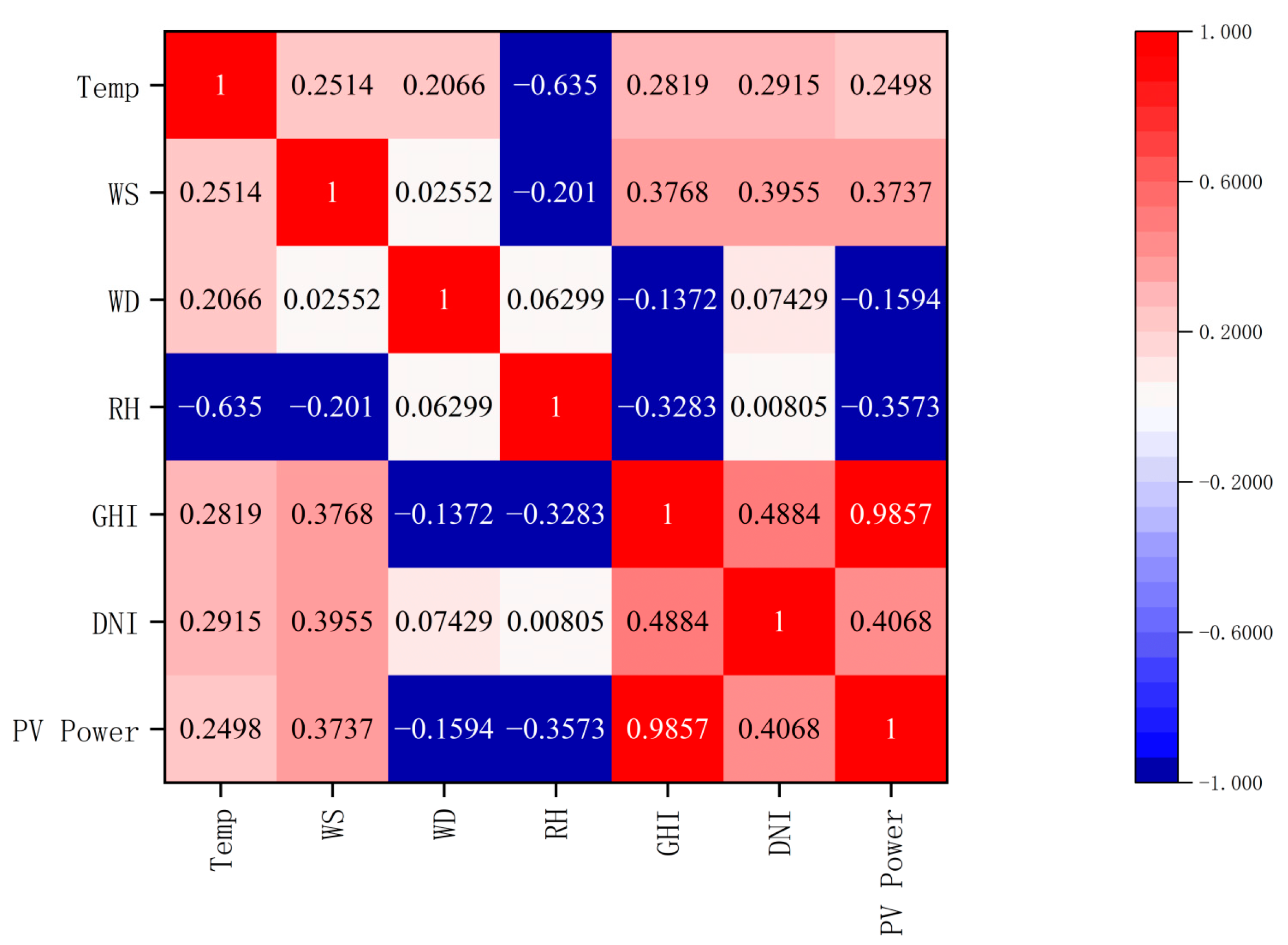
Figure 1. Alice Spring Spearman correlation analysis.

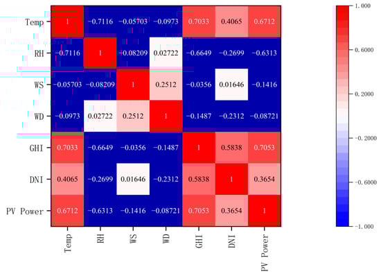
Figure 2. Kashgar Power Station Spearman correlation analysis.

Table 2. IDBO and DHKELM parameter settings.

Parameters	Values
Population size	30
Number of iterations	30
The random factor for the Levy flight strategy	0.6
The random value of the adaptive improvement	0.7
The number of hidden layer nodes	[1, 100]
Kernel weights	[1 × 10−3, 1 × 103]
Penalty coefficients	[1 × 10−3, 1 × 103]
Regularization terms	[0, 1]
Kernel settings	[1 × 10−3, 1 × 103]

Figure 1 and Figure 2 illustrate a high degree of correlation between PV power and total horizontal radiation, as indicated by the Spearman correlation coefficient. They reached values of 0.9857 and 0.7053, respectively. This indicates a highly positive correlation between PV power and total horizontal radiation. This is followed by the relative correlation between scattered radiation and PV power reaching 0.4068 and 0.3654. Weather temperature, weather relative humidity, and wind speed also exhibit a notable correlation. However, the correlation coefficients of wind direction are −0.1594 and −0.08721, respectively, indicating that the influence of wind direction on photovoltaic power generation can be ignored. Based on these findings, this paper selects total horizontal radiation, scattered radiation, weather temperature, weather relative humidity, and wind speed as the input features.

3. Preliminaries on Related Models

3.1. Variational Mode Decomposition

Variational modal decomposition (VMD) [19] is an adaptive data decomposition method that is widely used to decompose signal data into multiple discrete submodalities. In this paper, VMD is selected for the purpose of constructing a model for decomposing the PV power curve. The fundamental concept of VMD is to minimize the sum of the center frequencies of each modal component. This process can be regarded as a variational problem with constraints, and its model is formulated as follows:

$$\left\{\begin{array}{l}\underset{\left\{u_k\right\}\left\{{\omega }_k\right\}}{\min }\left.\left\{{\displaystyle \sum _{k=1}^k}||\left.{\partial }_t\left[\left(\delta (t\right)+{\displaystyle \frac{\mathrm{j}}{\pi t}}\right)u_k(t)\right]{\mathrm{e}}^{-\mathrm{j}{\omega }_{k}t}\right.|{|}_2^2\right\}\\ \mathrm{s}.\mathrm{t}.{\displaystyle \sum _{k=1}^K}{u}_k=f(t)\end{array}\right.$$

(2)

where $k$ is the number of modes; ${\partial }_t$ is the $t$-moment bias; ${\delta }_t$ is the Dirac distribution function; $u_k$ is the $k$th mode; ${\omega }_t$ is the center frequency; $\left|\right|.\left|\right|$ is the number of L2 paradigms; and $f(t)$ is the initial signal.

The conversion of the VMD model into an unconstrained optimization problem can be performed by incorporating Lagrange multipliers and quadratic penalty terms.

$$\left\{\begin{array}{l}L(\{u_k\},\{{\omega }_k\},\lambda )=\alpha {\displaystyle \sum _{k=1}^k||}{\partial }_t\left[\left(\delta (t)+{\displaystyle \frac{\mathrm{j}}{\pi t}}\right)\odot u_k\right]{\mathrm{e}}^{-\mathrm{j}{\omega }_{k}t}|{|}_2^2+\\ ||f(t)-{\displaystyle \sum _{k=1}^k}{u}_k|{|}_2^2+⟨\lambda (t),f(t)-{\displaystyle \sum _{k=1}^k}{u}_k(t)⟩\end{array}\right.$$

(3)

where λ is the Lagrange multiplier; α is the penalty factor; and $\odot$ is the convolution operator.

In the context of the VMD method, the alternating direction multiplier method can be employed for the resolution of the minimization problem, thereby facilitating its transformation into a selectable model.

3.2. Deep Hybrid Kernel Extreme Learning Machine

The kernel extreme learning machine (KELM) is a type of feedforward neural network that utilizes kernel functions. It is commonly applied to address both regression and classification tasks [20]. The primary concept is to address the issue of covariance resulting from the random generation and alteration of hidden layer weights through the introduction of kernel functions. The utilization of diverse kernel functions represents a valuable approach to enhancing the performance of KELM. However, a single kernel function is inadequate for comprehensively capturing the nonlinear characteristics inherent in PV power history data. In light of the aforementioned considerations, this paper introduces a hybrid kernel function that integrates the nonlinear characteristics of the polynomial kernel [21] with the global fitting capability of the RBF kernel function.

The polynomial kernel function expression is follows:

$$K_{Poly}(x_i,x_j)={(\beta *<x_i,x_j>+c)}^d$$

(4)

where $\beta$ is the scaling parameter; $<x_i,x_j>$ is the inner product of the vectors; $c$ is the constant term; and $d$ is the number of polynomials.

The RBF kernel function expression is as follows:

$$k_{\mathrm{RBF}}\left(x_i,x_j\right)=\exp \left({\displaystyle \frac{x_i-{x_j}^2}{{\gamma }^2}}\right)$$

(5)

where $k_{RBF}(x_i,x_j)$ is the RBF kernel function and $\gamma$ is the RBF kernel parameters.

The polynomial kernel function and the RBF kernel function are computationally independent, and so the two can be combined by linear weighting. The weighted kernel function formula can be expressed as follows:

$$k_D(x_i,x_j)=\epsilon \times k_{Poly}(x_i,x_j)+(1-\epsilon )\times k_{RBF}(x_i,x_j)$$

(6)

where $\epsilon$ is the hybrid kernel function weight coefficient.

When using the $k_D(x_i,x_j)$ kernel function instead of random mapping, the actual output of HKELM can be expressed as follows:

$$\left\{\begin{array}{l}f(x)=h(x)H^{\mathrm{T}}{\left(h{H}^{\mathrm{T}}+I/M\right)}^{-1}Y\hfill \\ \left[\begin{array}{c}{K}_{\mathrm{D}}\left(x,x_j\right)\\ ⋮\\ K_{\mathrm{D}}\left(x,x_n\right)\end{array}\right]{\left({\mathsf{\Omega }}_{\mathrm{ELM}}+I/M\right)}^{-1}Y\hfill \end{array}\right.$$

(7)

where ${\mathsf{\Omega }}_{\mathrm{ELM}}$ is the matrix of kernels; $M$ is the regularization factor; $Y$ is the target matrix; and $I$ is the unit matrix.

$$\left\{\begin{array}{l}{\mathsf{\Omega }}_{\mathrm{ELM}}=H{H}^{\mathrm{T}}\hfill \\ \mathsf{\Omega }(i,j)=h\left(x_i\right)h\left(x_j\right)=k\left(x_i,x_j\right)\hfill \end{array}\right.$$

(8)

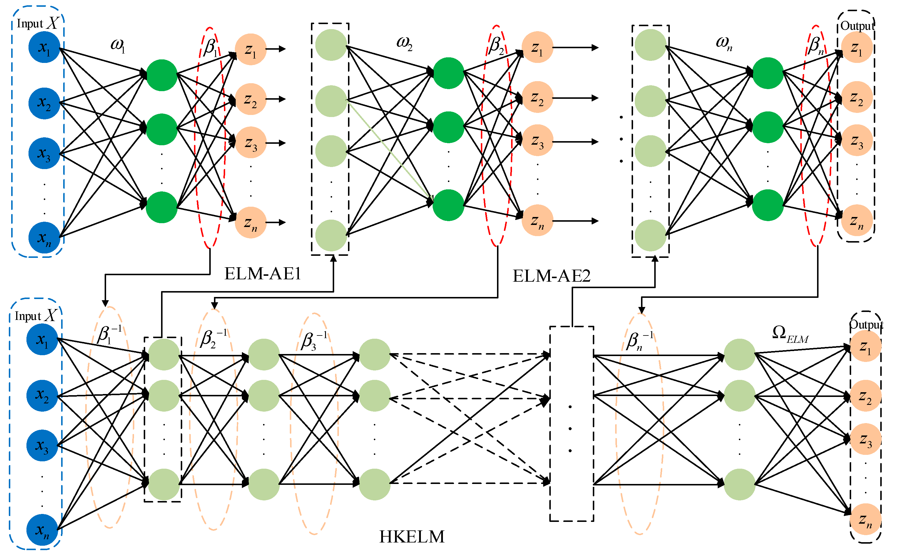
The AutoEncoder (AE) concept is incorporated into the ELM framework to maximize the potential of deep learning for feature extraction and the generalization of kernel functions. The network is capable of achieving the effective alignment of inputs and kernel outputs through training, enabling kernel function-based data reconstruction. A deep hybrid kernel extreme learning machine (DHKELM) is a deep learning method created by stacking multiple ELM-AEs. This structure enhances the network’s representational capacity by using multiple ELM-AEs to build a deep learning architecture that incorporates hybrid kernel functions, replacing the traditional stochastic mapping approach [22]. By employing a hierarchical unsupervised training method, DHKELM is capable of reducing reconstruction errors in a more effective manner and achieving a more precise alignment between input data and kernel output data. In comparison to traditional deep learning algorithms, this approach demonstrates a robust capacity for generalization while facilitating feature extraction. The model’s architecture is illustrated in Figure 3.

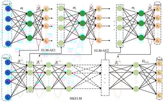
Figure 3. DHKELM network architecture diagram.

In the training process of the DHKELM network, the input data X are initially passed into the ELM-AE1 for training. This process leads to the computation of the corresponding output weight, denoted as ${\beta }_1$. This is subsequently transferred to the underlying hybrid kernel extreme learning machine (HKELM). Once the HKELM completes its training phase, the output matrix of the initial implicit layer is employed as the input and transmitted to the second self-encoder (ELM-AE2) for further training, thereby yielding the updated output weight ${\beta }_2$. Through several iterations, the weights are continuously optimized to form the ΩELM kernel matrix, which is then used to replace the stochastic matrix HHT. The final output result of DHKELM is obtained. By using DHKELM to train the VMD decomposed PV power components and meteorological factors, we are able to capture the high-dimensional features of the data, thereby improving the generalization and accuracy of the model’s prediction.

3.3. Dung Beetle Optimizer

The dung beetle optimizer (DBO) [23] is a recently proposed group intelligence algorithm, which was developed by Xue and Shen in 2022. Its design draws inspiration from the breeding and foraging behavior of dung beetles. In the DBO algorithm, the foraging area of the dung beetle is modeled using boundary selection. The upper and lower bounds of the variables of the objective function are set as the initial area for dung beetles to forage, and the activity area of the dung beetle population is restricted to that range. The foraging range of the dung beetle population is dynamically adjusted with its activity. The equation for its movement in space is expressed as follows:

$$x_i(t+1)=x_i(t)+c_1(x_i(t)-Lb)+c_2(x_i(t)-Ub)$$

(9)

where $x_i(t)$ is the position information of the $i$-th dung beetle in $t$ iterations, $c_1$ is a random number obeying a normal distribution, $c_2$ is a random vector in (0,1), and $Lb$ and $Ub$ are the upper and lower bounds of the dung beetle population movement, respectively. These are updated by Equation (10):

$$\left\{\begin{array}{l}Lb=\max (Xb(1-R),Lb)\hfill \\ Ub=\min (Xb(1+R),Ub)\hfill \end{array}\right.$$

(10)

where $R$ is a control parameter that increases linearly from 1 to infinity with the number of iterations. That is, $R={\displaystyle \frac{T_{\max }}{1-\mathrm{t}}}$, $t$ is the number of iterations; $T_{\max }$ is the maximum number of iterations; $Xb$ is the current local optimal position, which is updated by Equation (11):

$$Xb=x_i(t),\left(f\left(x_i(t)\right)>f(Xb)\right)$$

(11)

As the dung beetle moves, it gradually approaches and eventually searches for the global optimum by constantly exploring and searching for it.

4. Proposed Methodology

4.1. Improved the Dung Beetle Algorithm

The traditional dung beetle algorithm (DBO) has two significant limitations: a slow search speed and insufficient adaptability to dynamic changes in light. These shortcomings render the algorithm unsuitable for photovoltaic power prediction. This paper presents two improvement strategies that enhance the DBO algorithm’s search speed and adaptability to dynamic light changes.

4.1.1. Levy Flight Strategy

To prevent the algorithm from becoming stuck at a local optimum, Levy flight links are incorporated into the update formula. The incorporation of a Levy distribution for step-size generation adds more randomness and exploration capability. The long-tailed nature of the Levy distribution allows the dung beetle to cover a broader foraging area compared to the use of a fixed step size, thus increasing the likelihood of finding the globally optimal solution. The step-size equations for simulating the Levy flight process are as follows:

$$Levy(\beta )={\displaystyle \frac{\mu }{|v{|}^{-\beta }}}$$

(12)

where $Levy(\beta )$ is the obedience parameter that is the Levy distribution of $\beta$, $0<\beta <2$, and $\mu$ is the obedience to the $N(0,1)$ distribution. Equation (10) is updated by adding the Levy flight strategy.

$$x_i(t+1)=x_i(t)+c_1(x_i(t)-Lb(t))+c_2(x_i(t)-Ub(t))+\alpha Levy(\beta )r(t)$$

(13)

$$r(t)=\left\{\begin{array}{cc}0& rand<0.5\\ 1& rand\ge 0.5\end{array}\right.$$

(14)

where α is the scaling factor, taken as 0.01; $r(t)$ is a random function; and $rand$ is a randomly generated value within the range of [0, 1].

4.1.2. Adaptive Improvement Strategies

In the DBO iteration, the variation in the parameter $\epsilon$ affects the local exploitation and global exploration ability of the dung beetle. In the initial iteration, if the value of $\epsilon$ is insufficient, the search process will become excessively conservative, thereby impeding the comprehensive exploration of the solution space and adversely affecting the global search ability. Furthermore, if $\epsilon$ is set to a value that is excessively large, it may result in premature convergence in the later stages, thereby impeding the potential for the further enhancement of the optimal solution’s quality. To enhance the algorithm’s ability for global exploration and local optimization capacity, the feedback factor and nonlinear decreasing strategy are incorporated, as illustrated in Equations (15) and (16).

$$v_c={\left\{{\mathrm{e}}^{[(T_{\max }-t)/T_{\max }-1]1/{\mathrm{e}}^{-1}}\right\}}^4$$

(15)

$$\alpha =2.5{(1-{\displaystyle \frac{t}{T_{\max }}})}^{2/T_{\max }}$$

(16)

where $v_c$ is the feedback factor and α is the nonlinear decreasing parameter.

4.2. IDBO-DHKELM Prediction Model

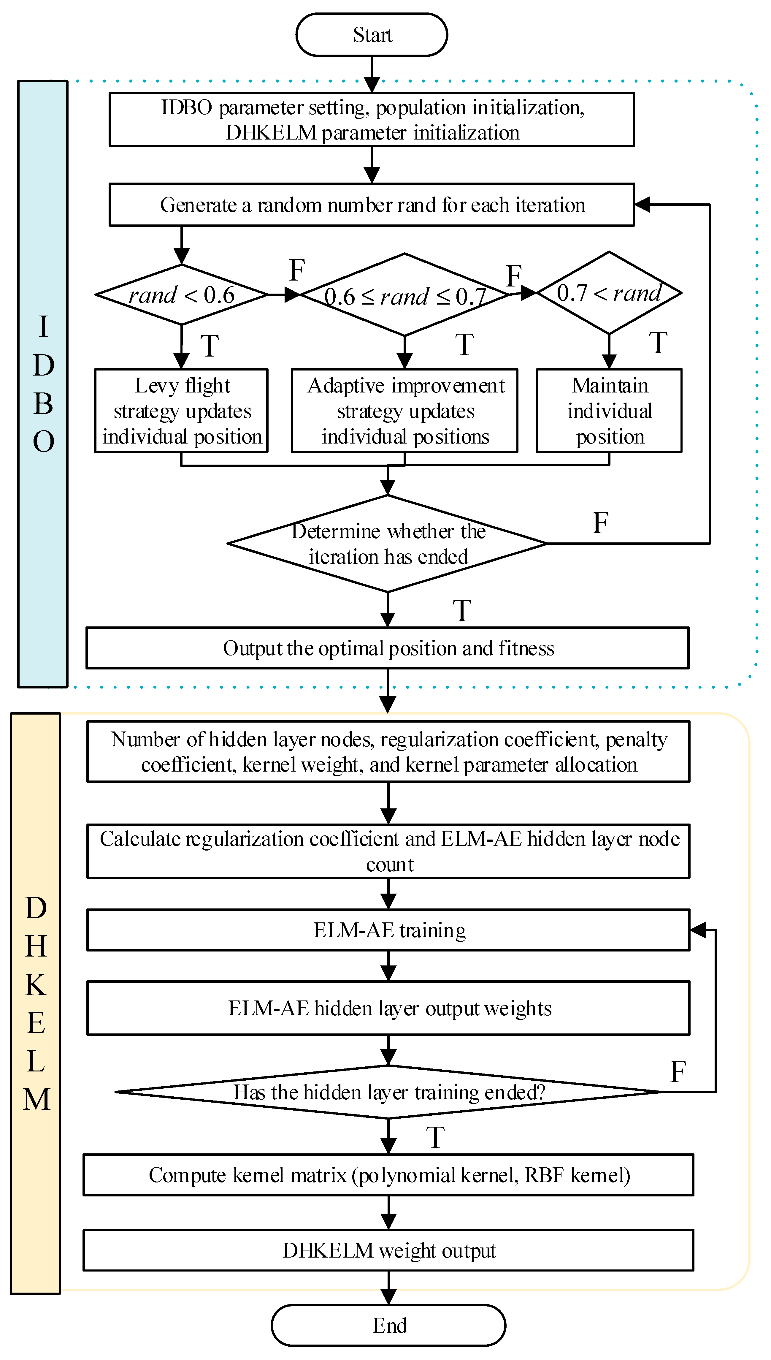
DHKELM comprises multiple ELM-AEs and HKELM. To maintain the generalization capacity of single-layer feedforward neural networks, a sig feature mapping approach is employed to train ELM-AEs. However, the role of the regularization coefficients and the number of nodes in the hidden layer is to suppress the overfitting of the ELMs and enhance their generalization ability. The penalty coefficients, kernel weights, and kernel parameters of the HKELM significantly influence the accuracy of PV prediction. Therefore, the IDBO algorithm was used to optimize parameters, including the number of hidden layer nodes, regularization factors, penalty terms, and kernel configurations.

(1)

Initialization stage: the population size, the number of iterations, the number of nodes in the hidden layer, regularization and penalty coefficients, the initial population positions, and the upper and lower bounds for the kernel parameters all need to be defined.

(2)

Individual position update: The dung beetles’ positions are adjusted using a Levy flight strategy combined with an adaptive improvement approach. After each iteration, the optimal fitness value, the worst fitness value, and the best position for that iteration are recorded. Once the iterations are completed, the optimal position and corresponding fitness value are output. The values at this optimal position represent the parameters to be optimized, including the number of hidden layer nodes, regularization coefficient, penalty coefficient, kernel weights, and other related parameters.

(3)

Upon the completion of the iteration, the optimal solution is obtained, and the DHKELM model is trained using this solution. Following the training phase, the final output weights of the DHKELM model are determined.

The overall flow chart is shown below.

4.3. VMD-IDBO-DHKELM Model

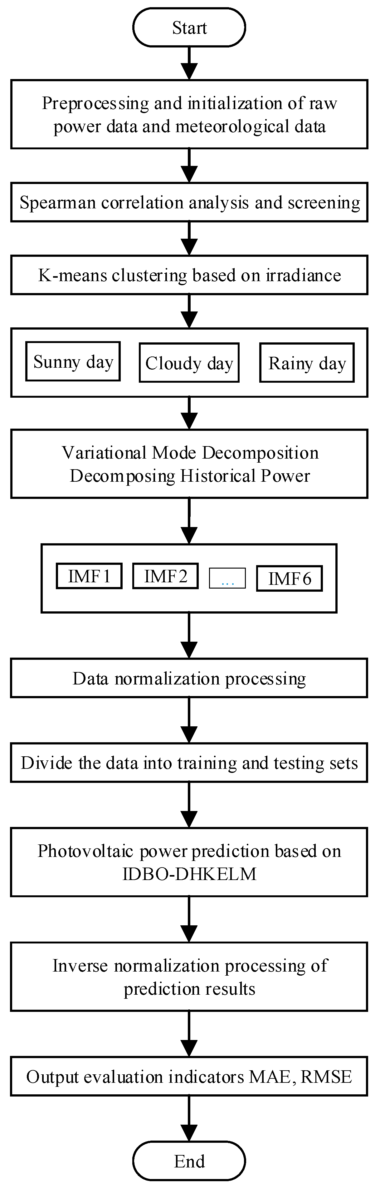
Due to the inherently variable nature of photovoltaic (PV) power generation, achieving a precise forecast of power output necessitates the application of a clustering algorithm, such as the K-means method, to categorize the total horizontal PV radiation data into distinct weather types. This is followed by a signal decomposition of power generation using the variational mode decomposition (VMD) technique. Subsequently, DHKELM is employed for prediction, and the hyperparameters of DHKELM are optimized by IDBO to establish a short-term PV power combination model based on optimized VMD-IDBO-DHKELM, which is shown as in Figure 4. And the whole flowchart is shown in Figure 5, which outlines the following steps:

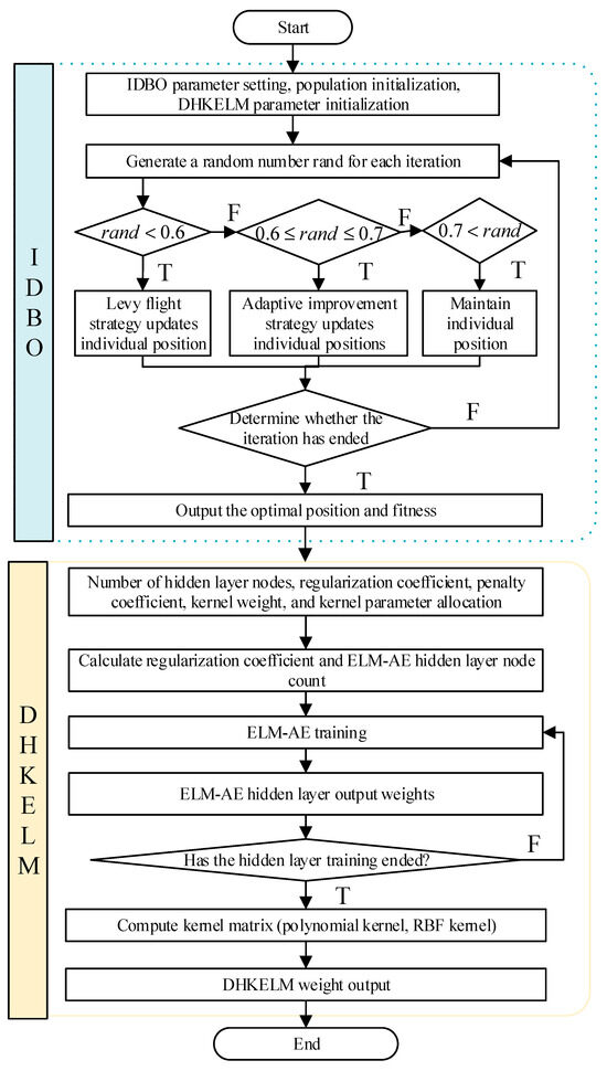
Figure 4. IDBO-DHKELM prediction model.

Figure 5. Flowchart of VMD-IDBO-DHKELM in similar day clustering.

(1)

The data are preprocessed by removing periods with no PV output and then splitting the dataset into training and testing subsets. The Spearman correlation coefficient (SCC) is used to identify the weather variables that are most relevant to PV power, which are then selected as input data.

(2)

The K-means algorithm groups the original data into categories based on similar weather patterns. The most recent day is assigned as the test set, with the other days serving as training data.

(3)

VMD of the clustered PV power is performed, and the decomposed data and meteorological factors are normalized to ensure consistency and input together as data into DHKELM.

(4)

The IDBO parameters are initialized, and the population size and the maximum number of iterations are set.

(5)

The DHKELM model is constructed—DHKELM predicts the processed training and test sets, and optimizes the hyperparameters of DHKELM using IDBO.

(6)

Once the training process is finished, the test set data are used to make predictions. The predicted results are then subjected to inverse normalization to obtain the final PV power forecasts, which are assessed using various performance metrics.

4.4. Evaluation Indicators

In this paper, Mean Absolute Error (MAE) and Root-Mean-Squared Error (RMSE) are used in the model to assess the accuracy of the model prediction results, and the formulas for the 2 metrics are shown in Equations (17) and (18).

$$MAE={\displaystyle \frac{1}{m}}{\displaystyle \sum _{i=1}^m\left|(y_i-\widehat{y_i}\right.}\left.)\right|$$

(17)

$$RMSE=\sqrt{{\displaystyle \frac{1}{m}}{{\displaystyle \sum _{i=1}^m(y_i-\widehat{y_i})}}^2}$$

(18)

where $y_i$ is the true value of PV power at moment i; $\widehat{y_i}$ is the corresponding predicted value; and $m$ is the number of samples for training.

5. Numerical Simulation Analysis

5.1. Data Preprocessing

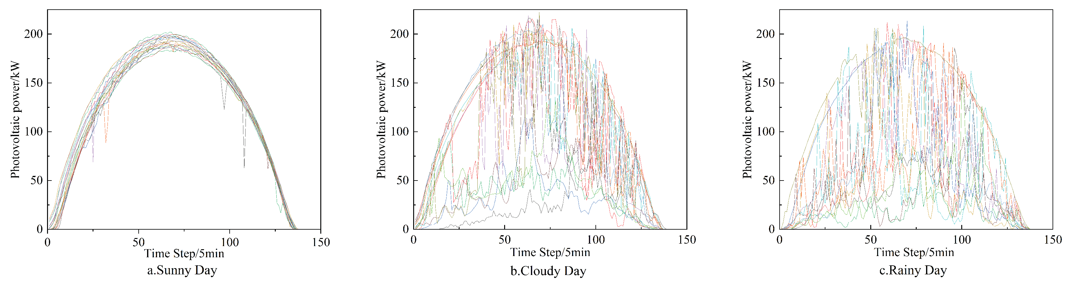
This paper presents a PV power prediction model that integrates the VMD-IDBO-DHKELM framework, designed to forecast PV power for the next one and three days (7:00 to 19:00), using historical and meteorological data from the Alice Spring and Kashgar PV power plants. The dataset was sampled at intervals of 5 and 60 min to assess the effectiveness and accuracy of VMD and IDBO in enhancing the deep hybrid kernel extreme learning machine (DHKELM) for PV power prediction. The prediction results for Alice Spring are presented in Figure 6. Weather is categorized into cloudy, sunny, and rainy conditions. Additionally, due to the specific sampling frequency and geographical factors in the Kashgar region, both sudden and non-sudden weather data are combined for prediction, thereby validating the robustness and generalization capability of the model.

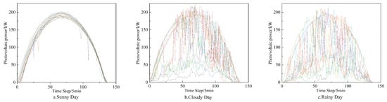
Figure 6. Clustering results of similar days.

5.2. Optimize Parameter Settings

An excessive value of k in the VMD may result in modal undercomposition. On the contrary, an excessively value of k may result in the severe overlapping of modal components or additional noise, leading to incorrect decomposition results. Therefore, it is very important to choose an appropriate k value. Taking the sunny day as an example, the center frequency method used determines the number of decomposed modes to be 5. The initial center frequency $\omega =1$, the convergence basis $r=1\times {10}^{-6}$, and the penalty factor $\alpha =12$.

Parameter settings about IDBO and DHKELM parameter settings [22] are shown in Table 2. The DHKELM model employs a decomposition approach, wherein the model is divided into three distinct components: sunny, cloudy, and rainy days. The activation function of ELM-AE is sig, while the polynomial kernel function and RBF are utilized as the kernel functions. The IDBO algorithm is used to optimize the model parameters, such as the number of hidden layer nodes, kernel weights, penalty coefficients, regularization terms, and kernel settings.

5.3. Result Analysis

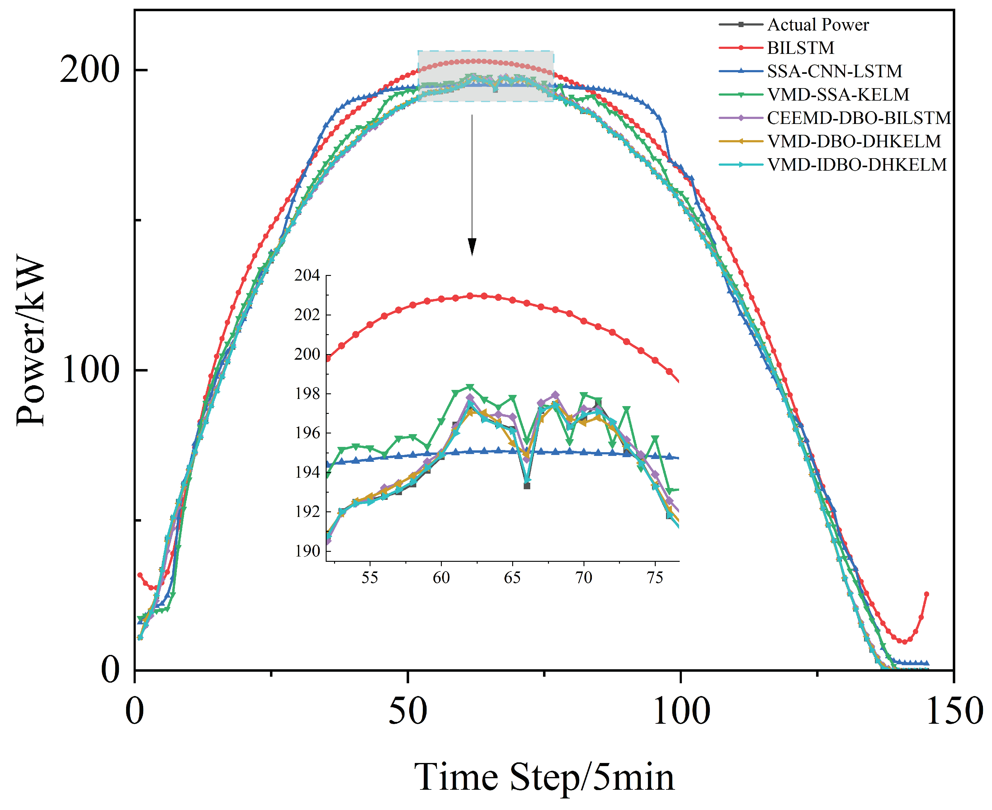
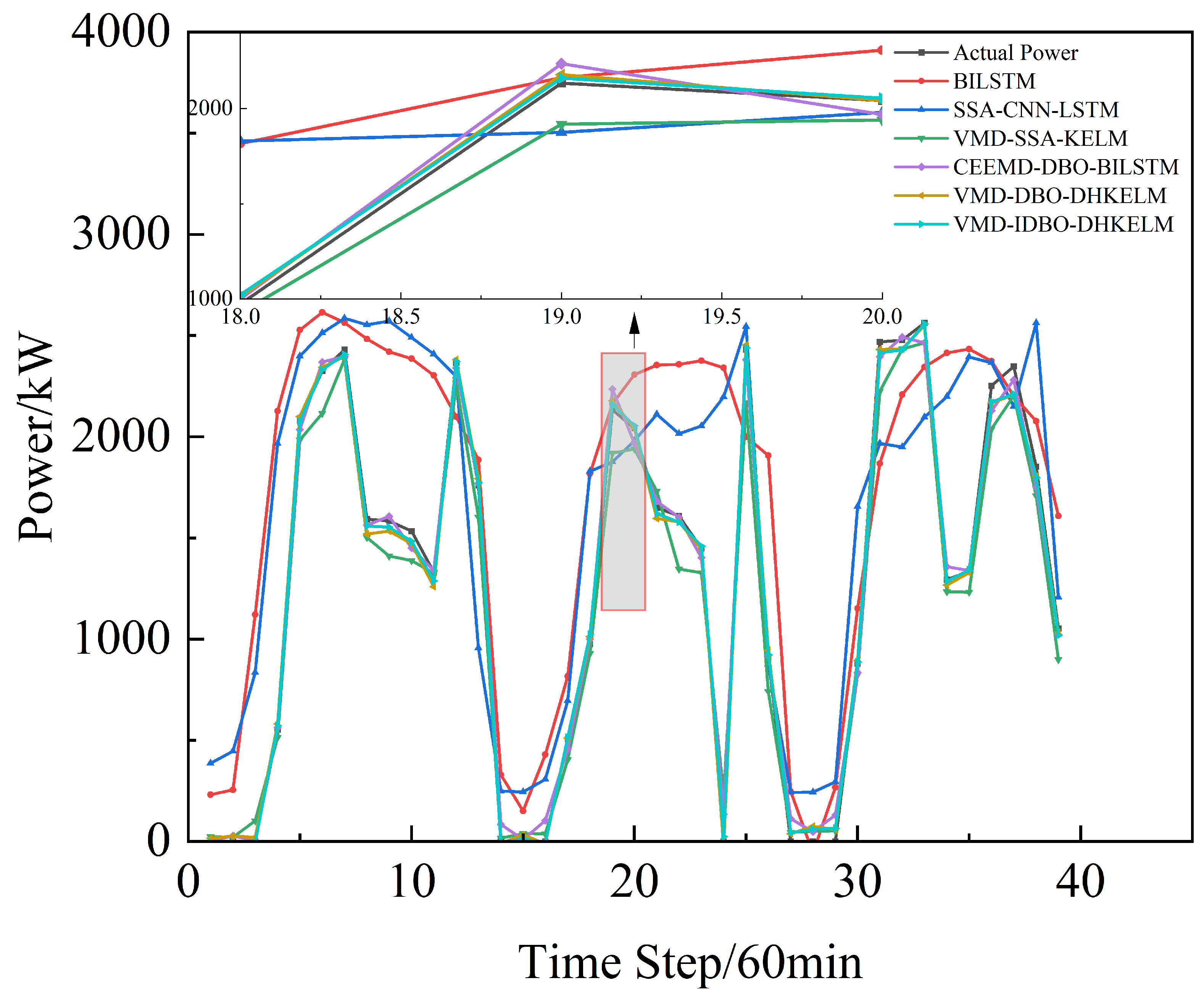
In order to ascertain the efficacy of the enhanced dung beetle algorithm in optimizing the DHKELM prediction model, a comparative analysis was conducted using four distinct methodologies: BILSTM, SSA-CNN-LSTM, VMD-SSA-KELM, CEEMD-DBO-BILSTM, and VMD-DBO-DHKELM. The results of the individual models’ predictions for Alice Spring, under sunny, cloudy, and rainy weather conditions, are presented in Figure 7, Figure 8 and Figure 9, respectively. Figure 10 depicts the results for Kashgar. Table 3 lists the evaluation indexes.

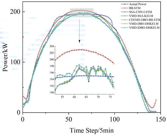
Figure 7. Sunny day forecast comparison.

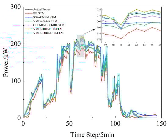
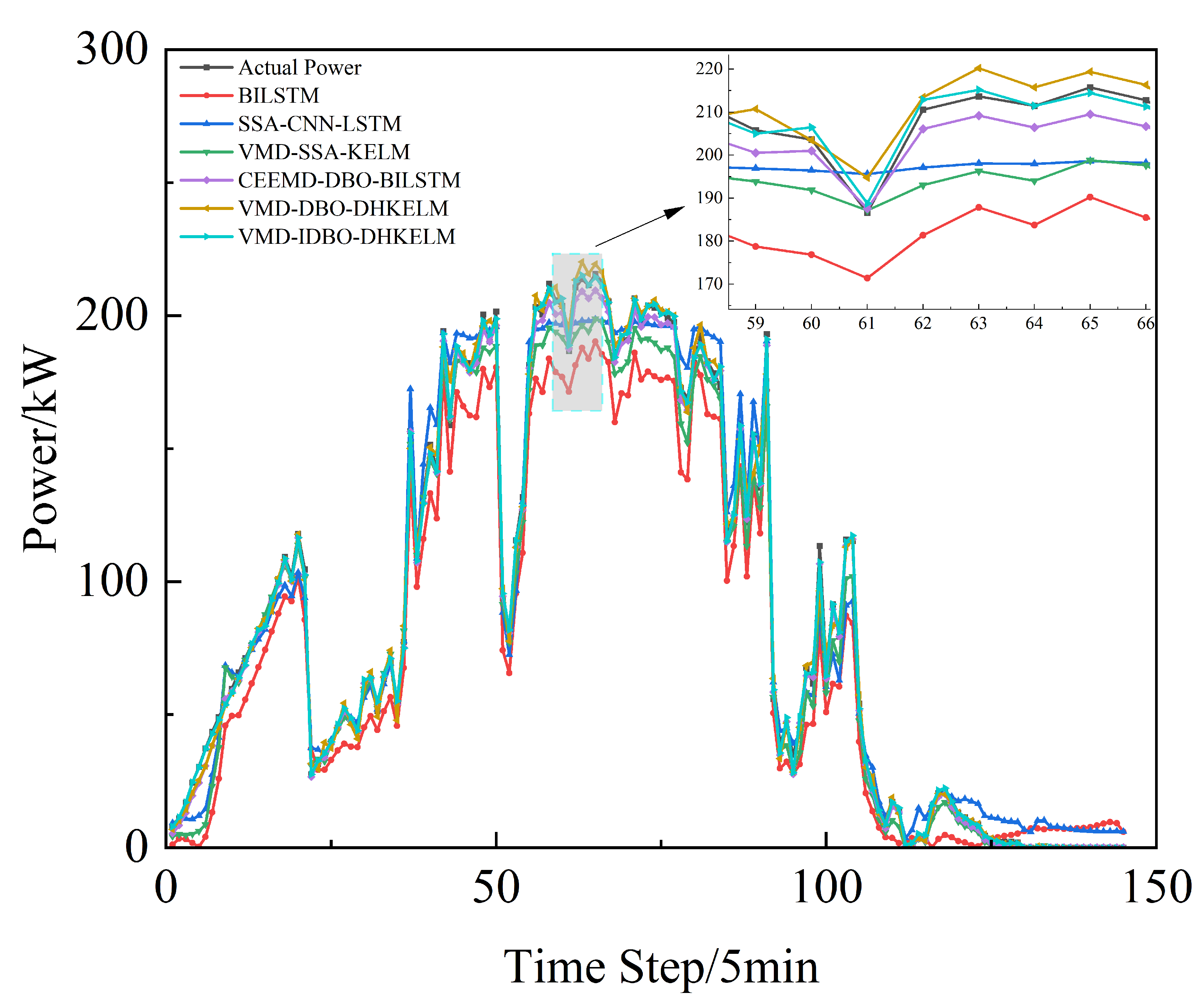
Figure 8. Cloudy day forecast comparison.

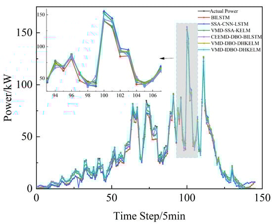
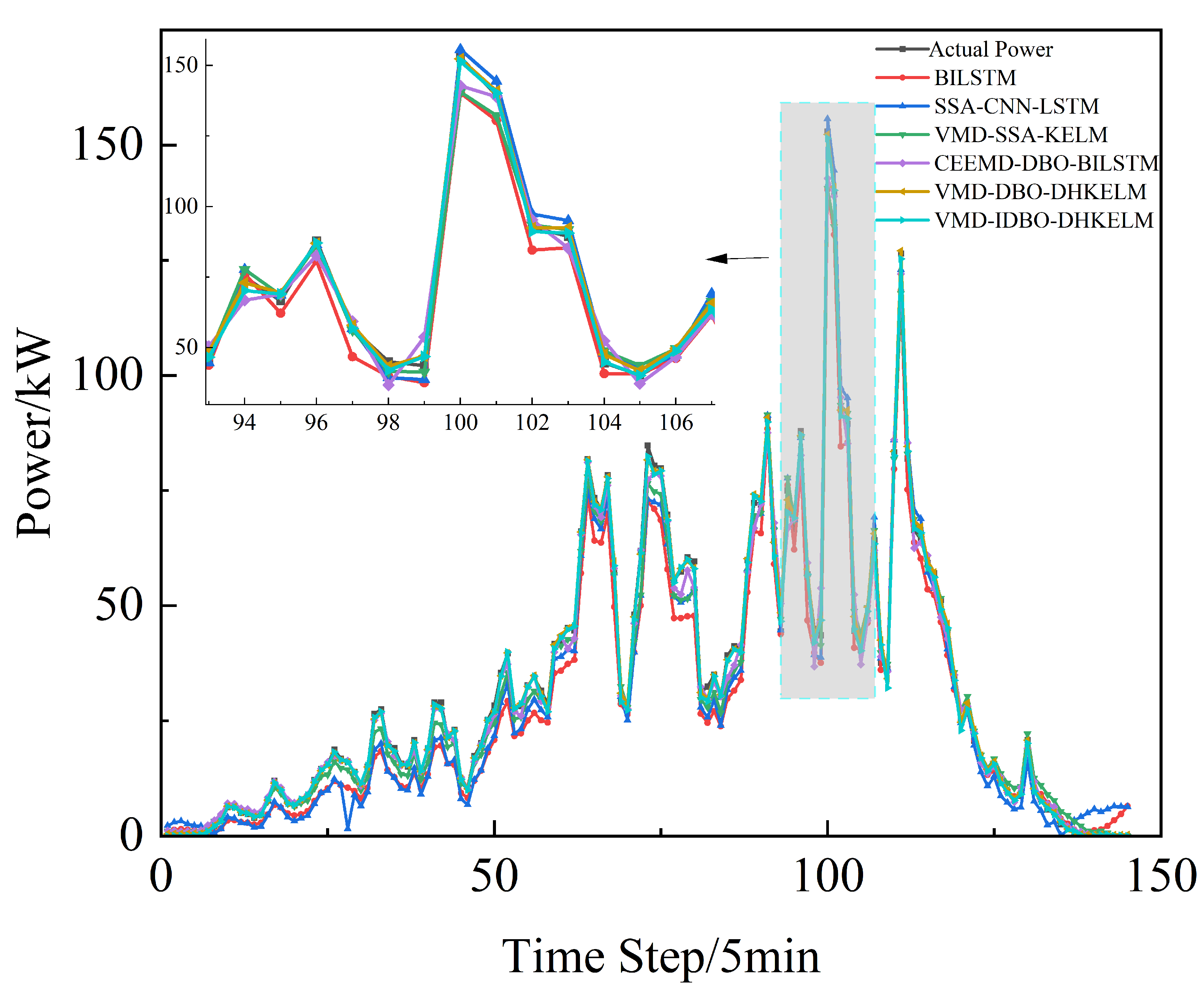
Figure 9. Rainy day forecast comparison.

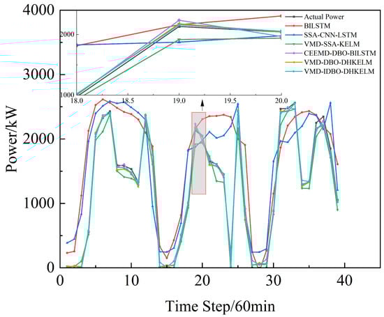
Figure 10. Kashgar prediction comparison.

Table 3. Evaluation metrics for each model.

Dataset Name	Weather	Evaluation	BILSTM	SSA-CNN-LSTM	VMD-SSA-KELM	CEEMD-DBO-BILSTM	VMD-DBO-DHKELM	VMD-IDBO-DHKELM
Alice Spring	Sunny	MAE	9.48	8.47	3.78	0.52	0.31	0.09
		RMSE	10.12	6.52	5.20	0.76	0.41	0.12
	Cloudy	MAE	15.42	9.32	6.61	3.03	2.31	1.51
		RMSE	17.21	7.48	8.88	4.49	2.93	2.06
	Rainy	MAE	5.37	4.84	2.42	1.73	0.78	0.75
		RMSE	5.84	4.25	3.16	2.62	1.18	1.14
Kashgar	Two months of data	MAE	556.46	532.25	85.19	50.75	35.65	28.25
		RMSE	729.10	659.36	110.08	63.90	44.61	38.83

As illustrated in the figure, the suggested power prediction model aligns well with the actual PV power output during sunny days, where there is less fluctuation in PV power. This suggests that the model is effective in capturing PV power trends under stable weather conditions. Even in more dynamic weather scenarios, such as cloudy or rainy days with significant PV power fluctuations, the model maintains high prediction accuracy, effectively tracking instantaneous power variations. Furthermore, as illustrated in Figure 10, the combined prediction model continues to deliver strong results using low-frequency historical power data, highlighting its robust generalization ability and minimal reliance on extensive data. The results in Table 3 further indicate that the proposed algorithm effectively models the output power curve, achieving high accuracy across a range of weather conditions, whether involving minimal fluctuations in PV or more complex weather patterns. This demonstrates its robust predictive capability under diverse environmental scenarios.

6. Conclusions

This paper presents a short-term prediction model for PV power generation, utilizing the VMD-IDBO-DHKELM framework and evaluating its performance through RMSE and MAE metrics. The simulation outcomes for scenarios, from both Australia and China, reveal that the proposed model surpasses other models in terms of accuracy, demonstrating its superior predictive capability and overall advantages. The main contributions of the research can be summarized as follows:

(1)

The historical PV data are clustered according to weather conditions (such as sunny, cloudy, or rainy) using the K-means algorithm. The Spearman correlation coefficient (SCC) is then applied to identify the key weather factors, helping to reduce the influence of irrelevant variables on the accuracy of the prediction.

(2)

By applying VMD to decompose the PV data, the non-stationary characteristics of the original dataset are effectively minimized, leading to improved prediction accuracy for the model.

(3)

Under all three weather conditions, the proposed combination model more accurately fits the PV power curve compared to several other combination models. This indicates that the proposed model exhibits significant strengths in both prediction accuracy and generalizability.

While the VMD-IDBO-DHKELM model improves prediction accuracy, it does have some limitations. Specifically, in terms of data feature selection, only five meteorological factors are considered as initial inputs in this study, and factors such as wind direction are excluded, which may have also impact on PV power generation to some extent. Future research could explore the inclusion of additional relevant factors to improve the precision and dependability of predictions. Moreover, the prediction results exhibit considerable variability under different weather conditions. Therefore, selecting appropriate prediction models or adjusting model parameters based on specific weather types, and comparing them with additional models, could further improve the practical applicability of PV power generation forecasting.

References

- Keddouda, A.; Ihaddadene, R.; Boukhari, A.; Atia, A.; Arıcı, M.; Lebbihiat, N.; Ihaddadene, N. Solar photovoltaic power prediction using artificial neural network and multiple regression considering ambient and operating conditions. Energy Convers. Manag. 2023, 288, 117186. [Google Scholar] [CrossRef]
- Li, N.; Li, L.; Zhang, F.; Jiao, T.; Wang, S.; Liu, X.; Wu, X. Research on short-term photovoltaic power prediction based on multi-scale similar days and ESN-KELM dual core prediction model. Energy 2023, 277, 127557. [Google Scholar] [CrossRef]
- Markovics, D.; Mayer, M.J. Comparison of machine learning methods for photovoltaic power forecasting based on numerical weather prediction. Renew. Sustain. Energy Rev. 2022, 161, 112364. [Google Scholar] [CrossRef]
- Pan, M.; Li, C.; Gao, R.; Huang, Y.; You, H.; Gu, T.; Qin, F. Photovoltaic power forecasting based on a support vector machine with improved ant colony optimization. J. Clean. Prod. 2020, 277, 123948. [Google Scholar] [CrossRef]
- Rao, Z.; Yang, Z.; Yang, X.; Li, J.; Meng, W.; Wei, Z. TCN-GRU Based on Attention Mechanism for Solar Irradiance Prediction. Energies 2024, 17, 5767. [Google Scholar] [CrossRef]
- Wu, H.; Liu, H.; Jin, H.; He, Y. Ultra-Short-Term Photovoltaic Power Prediction by NRGA-BiLSTM Considering Seasonality and Periodicity of Data. Energies 2024, 17, 4739. [Google Scholar] [CrossRef]
- Antonanzas, J.; Osorio, N.; Escobar, R.; Urraca, R.; Martinez-De-Pison, F.J.; Antonanzas-Torres, F. Review of photovoltaic power forecasting. Sol. Energy 2016, 136, 78–111. [Google Scholar] [CrossRef]
- Jia, P.; Zhang, H.; Liu, X.; Gong, X. Short-term photovoltaic power forecasting based on VMD and ISSA-GRU. IEEE Access 2021, 9, 105939–105950. [Google Scholar] [CrossRef]
- Zhang, M.; Han, Y.; Wang, C.; Yang, P.; Wang, C.; Zalhaf, A.S. Ultra-short-term photovoltaic power prediction based on similar day clustering and temporal convolutional network with bidirectional long short-term memory model: A case study using DKASC data. Appl. Energy 2024, 375, 124085. [Google Scholar] [CrossRef]
- Cui, S.; Lyu, S.; Ma, Y.; Wang, K. Improved informer PV power short-term prediction model based on weather typing and AHA-VMD-MPE. Energy 2024, 307, 132766. [Google Scholar] [CrossRef]
- Chen, G.; Zhang, T.; Qu, W.; Wang, W. Photovoltaic Power Prediction Based on VMD-BRNN-TSP. Mathematics 2023, 11, 1033. [Google Scholar] [CrossRef]
- Cai, Y.; Hao, S.; Wen, X.; Li, H.; He, X.; Chen, L.; Ren, J. Short-term power prediction by using least square support vector machine with variational mode decomposition in a photovoltaic system. IEEE Access 2023, 11, 143486–143500. [Google Scholar] [CrossRef]
- Zhang, C.; Peng, T.; Nazir, M.S. A novel integrated photovoltaic power forecasting model based on variational mode decomposition and CNN-BiGRU considering meteorological variables. Electr. Power Syst. Res. 2022, 213, 108796. [Google Scholar] [CrossRef]
- Wu, T.; Hu, R.; Zhu, H.; Jiang, M.; Lv, K.; Dong, Y.; Zhang, D. Combined IXGBoost-KELM short-term photovoltaic power prediction model based on multidimensional similar day clustering and dual decomposition. Energy 2024, 288, 129770. [Google Scholar] [CrossRef]
- Liu, Z.F.; Li, L.L.; Tseng, M.L.; Lim, M.K. Prediction short-term photovoltaic power using improved chicken swarm optimizer-extreme learning machine model. J. Clean. Prod. 2020, 248, 119272. [Google Scholar] [CrossRef]
- Zhou, Y.; Zhou, N.; Gong, L.; Jiang, M. Prediction of photovoltaic power output based on similar day analysis, genetic algorithm and extreme learning machine. Energy 2020, 204, 117894. [Google Scholar] [CrossRef]
- Zhang, X.; Grijalva, S. A data-driven approach for detection and estimation of residential PV installations. IEEE Trans. Smart Grid 2016, 7, 2477–2485. [Google Scholar] [CrossRef]
- Jebli, I.; Belouadha, F.-Z.; Kabbaj, M.I.; Tilioua, A. Prediction of solar energy guided by pearson correlation using machine learning. Energy 2021, 224, 120109. [Google Scholar] [CrossRef]
- Jiang, J.; Hu, S.; Xu, L.; Wang, T. Short-term PV power prediction based on VMD-CNN-IPSO-LSSVM hybrid model. Int. J. Low-Carbon Technol. 2024, 19, 1160–1167. [Google Scholar] [CrossRef]
- Chen, X.; Ding, K.; Zhang, J.; Han, W.; Liu, Y.; Yang, Z.; Weng, S. Online prediction of ultra-short-term photovoltaic power using chaotic characteristic analysis, improved PSO and KELM. Energy 2022, 248, 123574. [Google Scholar] [CrossRef]
- Long, H.; Zhang, Z.; Su, Y. Analysis of daily solar power prediction with data-driven approaches. Appl. Energy 2014, 126, 29–37. [Google Scholar] [CrossRef]
- Li, X.; Jin, W. A method for diagnosing rolling bearing faults based on SDAE-ADHKELM. Meas. Sci. Technol. 2022, 34, 025004. [Google Scholar] [CrossRef]
- Xue, J.; Shen, B. Dung beetle optimizer: A new meta-heuristic algorithm for global optimization. J. Supercomput. 2023, 79, 7305–7336. [Google Scholar] [CrossRef]
Disclaimer/Publisher’s Note: The statements, opinions and data contained in all publications are solely those of the individual author(s) and contributor(s) and not of MDPI and/or the editor(s). MDPI and/or the editor(s) disclaim responsibility for any injury to people or property resulting from any ideas, methods, instructions or products referred to in the content. |
© 2025 by the authors. Licensee MDPI, Basel, Switzerland. This article is an open access article distributed under the terms and conditions of the Creative Commons Attribution (CC BY) license (https://creativecommons.org/licenses/by/4.0/).