Cascade Hydropower Plant Operational Dispatch Control Using Deep Reinforcement Learning on a Digital Twin Environment

Abstract

In this work, we propose the use of a reinforcement learning (RL) agent for the control of a cascade hydropower plant system. Generally, this job is handled by power plant dispatchers who manually adjust power plant electricity production to meet the changing demand set by energy traders. This work explores the more fundamental problem with the cascade hydropower plant operation of flow control for power production in a highly nonlinear setting on a data-based digital twin. Using deep deterministic policy gradient (DDPG), twin delayed DDPG (TD3), soft actor-critic (SAC), and proximal policy optimization (PPO) algorithms, we can generalize the characteristics of the system and determine the human dispatcher level of control of the entire system of eight hydropower plants on the river Drava in Slovenia. The creation of an RL agent that makes decisions similar to a human dispatcher is not only interesting in terms of control but also in terms of long-term decision-making analysis in an ever-changing energy portfolio. The specific novelty of this work is in training an RL agent on an accurate testing environment of eight real-world cascade hydropower plants on the river Drava in Slovenia and comparing the agent’s performance to human dispatchers. The results show that the RL agent’s absolute mean error of 7.64 MW is comparable to the general human dispatcher’s absolute mean error of 5.8 MW at a peak installed power of 591.95 MW.

1. Introduction

Hydropower supplies nearly one-third of Slovenia’s electricity, with the eight-plant cascade on the Drava River alone contributing roughly 16% of national generation [1,2]. These facilities operate under tight constraints: reservoir levels must be managed to avoid spillage; turbine efficiencies vary nonlinearly with head and flow; and inter-plant water transfers create complex coupling. At the same time, energy traders set hourly schedules that dispatchers must meet in real time—often reacting to volatile market prices and stochastic inflows. Misalignment between trader bids and system physics can lead to costly penalties or even unplanned spills, posing both economic and environmental risks.

Traditional flow control schemes rely on simplified linear models or offline optimization that cannot capture the full cascade dynamics, forcing human dispatchers into heuristic adjustments under high uncertainty [3,4,5]. Data-driven digital twins show promise in faithfully reproducing these nonlinear behaviours without onerous modelling efforts [6], while reinforcement learning (RL) has demonstrated success in complex, continuous control domains such as robotics and process industries [7].

In this work, we unite these advances by developing a high-fidelity, data-driven simulation model (in the following referred to as a digital twin) of the Drava cascade and training RL agents, to manage flows under externally imposed trader schedules. Specifically, the agent methods are deep deterministic policy gradient (DDPG), twin delayed deep deterministic policy gradient (TD3), soft actor-critic (SAC), and proximal policy optimization (PPO). We show that our agents achieve a mean error of 7.64 MW—comparable to human dispatchers’ 5.8 MW—while preserving reservoir flexibility for future demands.

Hydropower operations have been advanced through a wide range of scheduling and control studies, spanning market participation optimization [8], RL formulations that incorporate inflow forecasts for cascaded scheduling [9], single-reservoir RL for operational policy learning and flow/spill control [10,11], intraday multi-reservoir management with actor–critic methods [12], simulation-based flexibility enhancement on digital twins [13], chance-constrained operation with safety back-offs [14], early RL applications on single reservoirs [15], long-term revenue-oriented scheduling with deep RL [16], multi-objective cascade optimization leveraging structural (monotonic) properties [17], foundational stochastic RL for multi-reservoir systems [18], short-term pumped-storage scheduling with deep deterministic policy gradients [19], comprehensive simulation–optimization surveys [20], and market participation designs for regulating hydropower [21]. Collectively, these contributions have improved planning and scheduling under uncertainty, demonstrated RL’s promise in water systems, and explored digital twin platforms and safety-aware formulations. These works predominantly optimize market or planning horizons [8,12,16,21], assume or embed inflow forecasts [9], focus on single-reservoir or idealized dynamics [10,11,13,15,19], or manage uncertainty through theoretical chance constraints and margins rather than real-time closed-loop control in full cascades [14,17,18,20].

In practice, dispatchers must react to two key uncertainties—future water inflows and trader-set power schedules—resulting in minute-level control under time-varying, unforecastable inputs. While a fully stochastic framework could model these uncertainties explicitly, formulating accurate probability distributions for inflows and market schedules is prohibitively complex. Instead, we pursue a model-free control approach: training actor-critic agents (DDPG, TD3, SAC, PPO) to learn optimal flow actions based solely on current reservoir states, treating inflows and schedules as exogenous disturbances.

Can such RL agents, trained on a high-fidelity, data-driven simulation model of the eight-plant Drava cascade, achieve a performance—in terms of mean error and reservoir safety—that approaches expert human dispatchers while handling real-world uncertainties? This question drives our work, motivating the development and evaluation of off-policy actor-critic algorithms for cascade flow and power operation control.

Our main contributions are as follows:

• High-Fidelity Data-Driven Simulation Model of the Drava Cascade. We construct a data-driven simulation of all eight hydropower plants on the Drava River—six impoundment and two diversion facilities—with accurate nonlinear head–flow maps, inter-plant hydraulic coupling, and reservoir dynamics, using operational records from DEM d.o.o. and HSE d.o.o. [22,23].
• Model-Free RL Controller. We cast real-time cascade flow control under externally imposed trader schedules as a continuous-state, continuous-action Markov decision process and train actor-critic agents (DDPG, TD3, SAC and PPO) that learn optimal dispatch policies directly from the digital twin, treating uncertain inflows and market targets as exogenous disturbances.
• Empirical Benchmarking Against Human Dispatchers. We perform a head-to-head comparison with historical dispatcher performance on the Drava system, demonstrating that our RL agents achieve an absolute mean error of 7.64 MW—closely approaching the 5.8 MW error of expert operators at a 591.95 MW installed capacity—while fully respecting operational and safety constraints.
• Robustness to Uncertainty. Without relying on explicit probabilistic models for future inflows or schedule deviations, our deterministic RL policies maintain high tracking accuracy and reservoir safety across diverse stochastic scenarios, reducing spillage and preserving system flexibility.

Related Work

Some works have similar approaches to our work but tackle the problem under different objectives and time scales than ours. For example, ref. [12] applies continuous-action RL to intraday hydropower scheduling, aiming to maximize economic profit from a multi-reservoir system. In their framework, the agent optimizes generation based on electricity prices and ramping constraints over each day, essentially treating the problem as a short-term revenue maximization task. This differs from our work in two key ways: (1) Reward formulation—in [12], the agent earns a reward proportional to income (energy × price), encouraging it to generate more when profitable. In contrast, our agent’s reward is the absolute deviation from a given schedule, emphasizing tracking accuracy over profit. (2) Externally imposed schedules vs. free optimization—We assume that the power set-point is mandated by an external trader or market operator and must be followed as closely as possible, whereas [12] allows the agent to decide the optimal generation profile to maximize returns. Notably, both approaches consider fine-grained, continuous control (including realistic constraints like water travel delays and gate limits), but the fundamental objective differs (compliance vs. optimization). Our work can be seen as a “digital dispatcher” scenario, closer to real operator duties, whereas [12] focuses on market-driven scheduling. This distinction is crucial: we demonstrate that even when the “optimal” schedule is fixed externally (and may at times be infeasible), an RL agent can intelligently adjust flows to minimize deviations, essentially acting as an automated cascade dispatcher. Prior RL studies have not addressed this real-time tracking problem—for instance, ref. [12] benchmarked its agents against MILP optimization and a greedy policy, but not against human operators. By targeting the dispatcher’s task, our work uniquely evaluates RL performance relative to actual human control behaviour.

Another interesting work for us is [16], which provides a complementary contrast in terms of time scale and scope. The authors explored a deep RL approach (soft actor-critic) for long-term hydropower scheduling, where the objective is to optimize yearly revenue by deciding week-to-week reservoir releases. Their agent learned when to release water versus store it, balancing immediate generation at the current electricity price against the potential value of water in the future. This long-term planning scenario differs from our real-time dispatch setting both mathematically and conceptually. Mathematically, Riemer-Sørensen’s reward function integrates economic returns over a yearly horizon, whereas we formulate a stepwise penalty on instantaneous schedule error. Their state space includes coarse weekly inflow and price levels, while ours comprises high-frequency reservoir and flow states needed for minute-level control. Conceptually, ref. [16]’s RL policy plays a strategic planning role (analogous to optimizing storage and generation over seasons), whereas our RL policy functions as an operational controller that fine-tunes outputs in real time to meet a target trajectory. The two approaches are complementary: a long-term RL scheduler could set targets that a real-time RL dispatcher then tracks.

It is also instructive to compare our approach to RL methods for single-reservoir control. Ref. [11] recently applied DDPG, TD3 and SAC to “fill-and-spill” reservoir operation, where the agents learned to meet downstream water demands and avoid spills in a standalone reservoir system. Their reward combined multiple terms to penalize unmet demand and excessive release, effectively training the policy to meet operational targets (water supply and flood control) reliably. This aligns with our finding that advanced policy-gradient agents can satisfy operational constraints; indeed, ref. [11] reports that TD3 and SAC agents kept the reservoir within target levels and met demands consistently. The key difference is scale and context: they addressed one reservoir with multi-objective targets, while we handle an eight-plant cascade tracking an externally set power schedule. Additionally, our work explicitly contrasts the RL policy’s behaviour with human actions, an angle not explored by [11] (who compared RL algorithms with each other).

In summary, across these related studies—whether focusing on economic optimization, long-term scheduling, or single-reservoir control—our work is differentiated by its real-time cascade control objective and the benchmark against actual dispatcher performance. A detailed, result-based comparison and state representation discussion of [11,12,16] appears in Section 3.5.

As shown in

Table 1. Related work areas and methods.

Ref.	Authors and Year	Focus Area	RL Method	System Type	Key Contributions/Notes
[8]	Wu et al. (2022)	Energy market participation optimization	N/A *	Cascaded	Presents a stochastic decomposition model that optimizes monthly contract and day-ahead spot market.
[9]	Xu et al. (2020)	Scheduling with inflow forecast	Deep Q-network (DQN)	Cascaded	Uses inflow forecasting for hydropower scheduling; simplified dynamics.
[10]	Xu et al. (2021)	Optimal hydropower operation	DQN	Single reservoir	Generalized operation policy learning on simplified discrete models.
[11]	Sadeghi Tabas & Samadi (2024)	Fill-and-spill flow control	TD3 + SAC	Single reservoir	Trains policy for flow/spill management on an isolated reservoir.
[12]	Castro-Freibott et al. (2025)	Intraday multi-reservoir scheduling	A2C + PPO + SAC	Cascaded	Short-term energy market operation.
[13]	Tubeuf et al. (2023)	Enhancing flexibility via Digital Twin	DDPG	Single hydropower plant	Simulation-based control; optimizes for system flexibility, not real dispatch.
[14]	Mitjana et al. (2022)	Chance-constrained hydropower operation	Policy gradient method	Multi-reservoir	Addresses uncertainty and safety through backoff margins.
[15]	Castelletti et al. (2010)	Optimal water reservoir operation	Fitted Q-iteration	Reservoir	Early fitted Q-iteration method; long-term scheduling focus.
[16]	Riemer-Sørensen et al. (2020)	Long-term scheduling of hydropower production—optimizing yearly revenue	SAC	Single reservoir	SAC algorithm can be successfully trained on historical Nordic market data to generate effective long-term release strategies.
[17]	Li et al. (2025)	Water availability optimization	Improved reinforcement learning	Multi-reservoir	Increased computation efficiency for optimizing water availability.
[18]	Lee & Labadie (2007)	Stochastic multi-reservoir optimization	Q-learning	Multi-reservoir	One of the earliest uses of RL in water systems; focuses on inflow uncertainty.
[19]	Ma et al. (2025)	Short-term pumped-storage scheduling	DDPG	Single plant	Uses DDPG for accurate, constraint-aware, water-efficient pumped-storage scheduling.
[20]	Rani & Moreira (2010)	Simulation–optimization modelling review	N/A	N/A	Foundational survey; sets the stage for RL and hybrid models.
[21]	Xie et al. (2025)	Hydropower plants participation in the spot market	N/A	N/A	Designs spillage management, compensation; separate bidding; long-term supply constraints integrated.
[Our work]		Cascade hydropower flow and power operation control	DDPG + TD3 + SAC + PPO	Cascaded	Using RL to approximate the current human dispatcher for simulation and analysis.

* N/A: Not applicable.

, most prior approaches focus on forecasting, theoretical constraints, or idealized operations, whereas our agent learns to perform in a highly nonlinear environment approximated from real data, reflecting the true complexities faced by dispatchers. Relative to the extensive review [22], our study targets an underrepresented problem: real-time, model-free deep RL for a multi-reservoir cascade that tracks externally imposed power schedules. Most surveyed work in [22] treats long-term planning or profit maximization, often single reservoirs or simplified cascades, with few real-time dispatch studies and none benchmarking against human operators. Our digital twin, constraint-aware controller runs sub-hourly, respects ramping/level limits, models hydraulic coupling and delays, and minimizes schedule deviation rather than maximizing energy. This directly fills gaps on real-time operation, operational compliance, and practical benchmarking, positioning our contribution as a pragmatic “digital dispatcher”.

2. Methodology

2.1. Cascade Hydropower Plant System

The Drava River (shown in Figure 1) traverses 133 km of north-eastern Slovenia, dropping 148 m between the Austrian border and the Croatian frontier. The mean annual discharge within this reach is 297 ${\displaystyle \frac{m^3}{s}}$, with flood peaks exceeding 2800 ${\displaystyle \frac{m^3}{s}}$ [2]. Thanks to this steady alpine runoff and moderate gradient, eight hydropower plants (HPP) form a fully cascaded system operated by DEM d.o.o.; a further thirteen Drava plants lie upstream in Austria and downstream in Croatia. The characteristics of the hydropower plants are shown in

Table 2. Basic hydropower plant characteristics.

Plant	Year Build	Rated Power (Rounded MW)	Reservoir Length (km)	Usable Reservoir Volume $({10}^6$ m3)	Maximal Turbine Flow $(\frac{{\mathit{m}}^3}{\mathit{s}})$
Dravograd	1944	26	10.2	1.045	420
Vuzenica	1953	56/60	11.9	1.807	550
Vuhred	1956	72	13.1	2.179	297
Ožbalt	1960	73	12.7	1.400	305
Fala	1918	58	9.0	0.535	260
Mariborski Otok	1948	60	15.5	2.115	270
Zlatoličje *	1969	136	6.5 + 17	0.3600	577
Formin *	1978	116	7.0 + 8.5	4.498	548

* Zlatoličje and Formin are diversion plants supplied by concrete canals parallel to the natural riverbed.

.

2.2. Digital Twin

The digital twin of the cascade set of hydropower plants was modelled as a mixture of hard constraints and data-based approximations, and is generally founded on [23,24] and contains the same principles as [3]. Firstly, we will present the assumptions and hard constraints we used in the study.

Calculating the hypothetical new usable water volume $V_{i,t}^{use,hyp}$ is performed by summing all water flows $Q_{i,t}^{net,real}$ during the timestep t for each reservoir i separately and adding it to the total volume of usable water in the reservoir from the previous step $V_{i,t-1}^{use}$.

$$V_{i,t}^{use,hyp}=V_{i,t-1}^{use}+\sum _{t=t-1}^t{Q}_{i,t}^{net,real}$$

(1)

This is necessary to calculate the constraint violations. Each reservoir has a hard safety constraint for the water level and water level change speed. We will assume those constraints cannot be broken; thus, all water inflow that results in the water level rising above the limits, denoted by the maximum volume of usable water $V_i^{max}$, is treated as overflow $Q_t^{over,lvl}$.

$$Q_{i,t}^{over,lvl}=\left\{\begin{array}{c}{\displaystyle \frac{V_{i,t}^{use,hyp}-V_i^{max}}{∆t}}, \\ 0,\end{array}\right. \begin{array}{c} if V_{i,t}^{use}>V_i^{max}\\ otherwise.\end{array}$$

(2)

Conversely, all reservoir outflows resulting in the usable water volume and dropping below the minimum $V_i^{min}$ allowed will be cut-off $Q_{i,t}^{out c-o,lvl}$. Outflows $Q_{i,t}^{out}$ are controlled by the RL agent and are considered the volume of water released over the turbines.

$$Q_{i,t}^{out c-o,lvl}=\left\{\begin{array}{c}{\displaystyle \frac{V_i^{min}-V_{i,t}^{use}}{∆t}}, \\ 0,\end{array}\right.\begin{array}{c} if V_{i,t}^{use}<V_i^{min}\\ otherwise.\end{array}$$

(3)

The net difference between the reservoir inflow and outflow that violates the water change speed constraints will limit either water inflow $Q_{i,t}^{over,rate}$ or outflow $Q_{i,t}^{out c-o,rate}$ until the value falls within the accepted range. Each reservoir $i$ has a set empirically allowed net flow of water $Q_i^{net,max}$.

$$Q_{i,t}^{over,rate}=\left\{\begin{array}{c}{Q}_{i,t}^{net}-Q_i^{net,max}, \\ 0,\end{array}\right.\begin{array}{c} if Q_{i,t}^{net}>Q_i^{net,max}\\ otherwise.\end{array}$$

(4)

$$Q_{i,t}^{out c-o,rate}=\left\{\begin{array}{c}{Q}_{i,t}^{net}+Q_i^{net,max}, \\ 0,\end{array}\right.\begin{array}{c} if Q_{i,t}^{net}<{-Q}_i^{net,max}\\ otherwise.\end{array}$$

(5)

To obtain the total overflow $Q_{i,t}^{over}$ in each reservoir, we simply sum the overflow caused by positive water level violations $Q_{i,t}^{over,lvl}$ and the overflow that resulted from the water level rising too fast $Q_{i,t}^{over,rate}$.

$$Q_{i,t}^{over}=Q_{i,t}^{over,lvl}+Q_{i,t}^{over,rate}$$

(6)

Similarly, to calculate the water outflow cut-off amount $Q_{i,t}^{out c-o}$, we add together the required cut-off amount caused by negative water level violations $Q_{i,t}^{out c-o,lvl}$ and the amount of outflow reduction required to stop the water level dropping too fast $Q_{i,t}^{out c-o,rate}$.

$$Q_{i,t}^{out c-o}={Q_{i,t}^{out c-o,lvl}+Q}_{i,t}^{out c-o,rate}$$

(7)

After applying all constraints to the original net water flow, we obtain the actual reservoir water flow $Q_{i,t}^{net,real}$, where the inflow $Q_{i,t}^{in}$ is the sum of the overflow $Q_{i-1,t}^{over}$ and turbine flow from the previous reservoir $Q_{i-1,t}^{turb}$.

$$Q_{i,t}^{turb}=Q_{i,t}^{out}-Q_{i,t}^{out c-o}$$

(8)

$$Q_{i,t}^{in}=Q_{i-1,t}^{over}+Q_{i-1,t}^{turb}$$

(9)

$$Q_{i,t}^{net,real}=Q_{i,t}^{in}-Q_{i,t}^{over}-Q_{i,t}^{out}+Q_{i,t}^{out c-o}$$

(10)

$$V_{i,t}^{use}=V_{i,t-1}^{use}+{\sum }_{t=t-1}^t{Q}_{i,t}^{net,real}$$

(11)

The total volume of usable water is then input into an empirical polynomial derived from provided measurement data to calculate the new headwater level in the reservoir $h_{i,t}^{head}$. For example, when the usable water volume is 0, the polynomial returns the minimum headwater level:

$$h_{i,t}^{head}= \sum _{j=1}^3{C}_j·{\phi }_j\left(V_{i,t}^{use}\right),$$

(12)

where

• ${\phi }_1={\left(V_{i,t}^{use}\right)}^2$,
• ${\phi }_2=V_{i,t}^{use}$,
• ${\phi }_3=1$.

The coefficients $C_j$ (for $j$ = 1, 2, 3) are unique and derived from measurement data for each reservoir [23,24]. With the static headwater levels calculated, we can move to calculating the hydraulic head. The measurement data exposes a highly nonlinear relationship between the tailwater right after the hydropower dam $h_{i,t}^{tail}$, the headwater level at the end of the reservoir (right upstream of the next dam) $h_t^{head}$, and the amount of water flowing into the reservoir $Q_{i,t}^{in}$. The rise in tailwater proves to be significant at higher inflow rates. This in turn highly affects the hydraulic head $∆H_{i,t}$, which is the difference between the upstream waterhead level and downstream tailwater level.

$$∆H_{i,t}=h_{i,t}^{head}-h_{i+1,t}^{tail}$$

(13)

Based on the measurement data, we used approximate polynomials that describe this relationship. The degree of the polynomials varies depending on the complexity of the data, but all generally keep the same form:

$$h_{i,t}^{tail}= \sum _{j=1}^6{K}_j·{\psi }_j\left(Q_{i,t}^{in},h_{i,t}^{head} \right),$$

(14)

where

• ${\psi }_1={\left(Q_{i,t}^{in}\right)}^2$,
• ${\psi }_2=Q_{i,t}^{in}·h_{i,t}^{head}$,
• ${\psi }_3={\left(h_{i,t}^{head}\right)}^2$,
• ${\psi }_4=Q_{i,t}^{in}$,
• ${\psi }_5=h_{i,t}^{head}$,
• ${\psi }_6=1$.

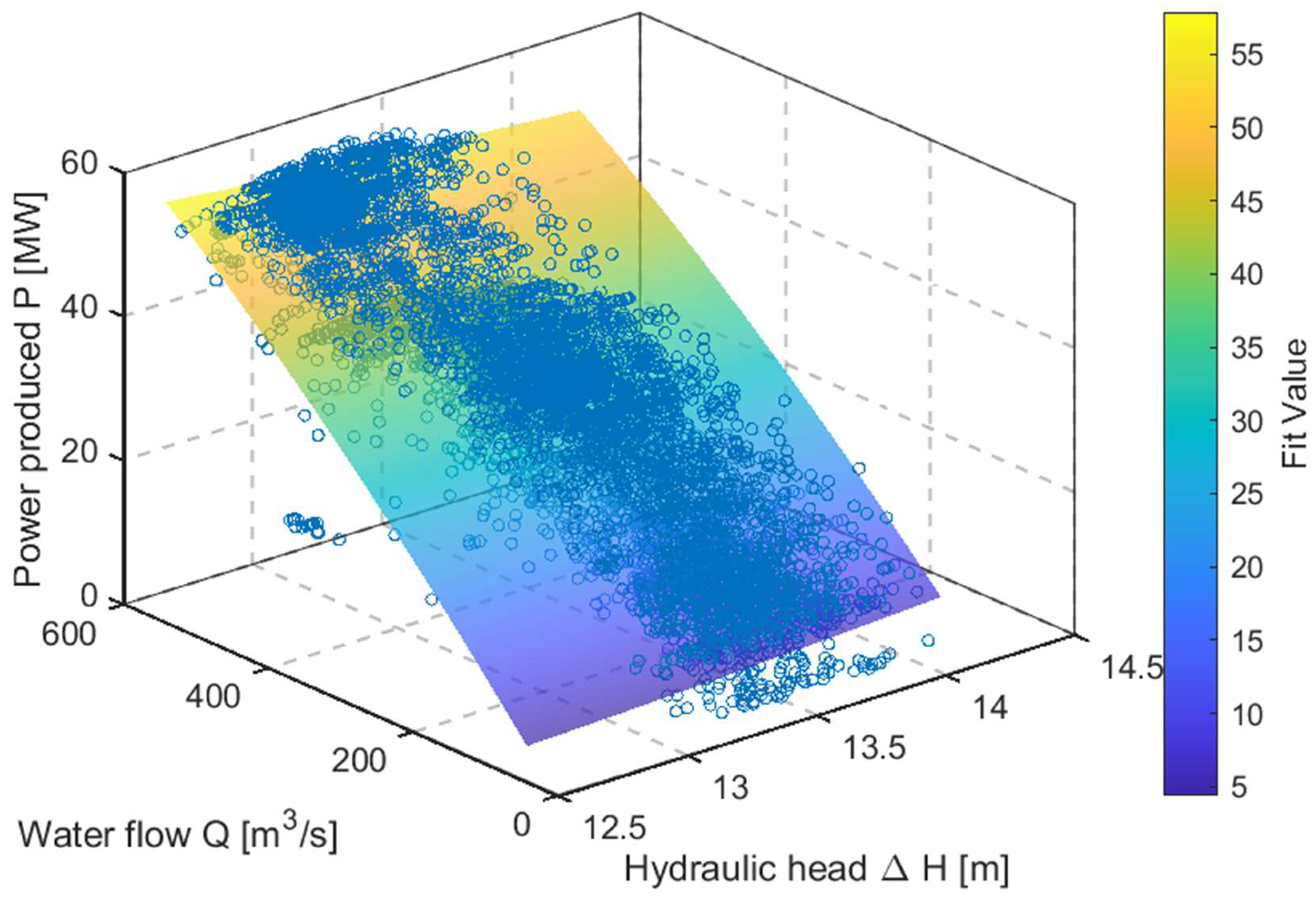
The coefficients $K_j$ (for $j=1, \dots , 6)$ are once again all unique to each hydropower plant reservoir [23,24]. In some examples, it became evident that some polynomial approximations have difficulties being inserted into the data since the data points have a very large dispersion, possibly due to the occurrence of seiches within the reservoirs (example of data fitting shown in Figure 2). The inclusion of seiche simulations could improve the accuracy; however, it would require computationally intensive hydraulic simulations that are beyond the scope of this work.

Once we have calculated the hydraulic head and allowed turbine water flow, we can determine the power produced by the hydropower plant. After analyzing the operations of power production provided by dispatchers, it was noted that they generally distribute the power production load between turbines to keep them operating in ranges that incur the least stress on individual components. To that end, we will not delve into optimal turbine load distribution analysis and instead use the measurement data of water flow and power production to generalize the amount of power produced $P_{i,t}^{prod}$ depending on the turbine water flow and hydraulic water head. Effectively, we treat each power plant as a single turbine with the combined operational characteristics of all individual turbines. Once again, we used polynomials that approximately fit the data:

$$P_{i,t}^{prod}= \sum _{j=1}^9{X}_j·{\chi }_j\left(∆H_{i,t},Q_{i,t}^{turb} \right),$$

(15)

where

• ${\chi }_1={(∆H_{i,t})}^3$,
• ${\chi }_2={(∆H_{i,t})}^2·Q_{i,t}^{turb}$,
• ${\chi }_3=∆H_{i,t}·{\left(Q_{i,t}^{turb}\right)}^2$,
• ${\chi }_4={(∆H_{i,t})}^2$,
• ${\chi }_5=h_{i,t}^{head}$,
• ${\chi }_6={\left(Q_{i,t}^{turb}\right)}^2$,
• ${\chi }_7=∆H_{i,t}$,
• ${\chi }_8=Q_{i,t}^{turb}$,
• ${\chi }_9=1$.

The degree of the polynomial and coefficients $X_j$ (for $j$ = 1, …, 9) is again identified based on measurement data [23,24]. This polynomial is essentially the power curve function (example of data fitting shown in Figure 3).

The bigger problem turned out to be the water inflow data in the first power plant. The most reliable data was the water flow of the previous power plant located in Austria. However, this data is missing the extra inflows into the river from smaller streams. These individually do not pose a significant contribution to the volume of water, but together they can have a meaningful impact on the potential of power production. We noticed this when running the first few simulations of cascade operation. The models of direct precipitation, surface runoff, groundwater discharge, smaller torrential stream inflows, and other additional sources are currently beyond the scope of this model. Thus, we chose an estimated constant additional flow at the start of the cascade of $50{\displaystyle \frac{m^3}{s}}$. This was based on estimates from operational logs and ARSO—National Meteorological Service of Slovenia data (National Meteorological Service of Slovenia).

2.3. Reinforcement Learning

Both reinforcement learning algorithms are custom-built in MATLAB R2023b. They are directly based on the original works describing their structure [25,26,27,28]. Neural networks were developed and trained using MATLAB’s Deep Learning Toolbox Deep Learning Toolbox and Statistics and Machine Learning Toolbox (MathWorks, Natick, MA, USA Statistics and Machine Learning Toolbox). These toolboxes provided the necessary functions for network creation, training, and evaluation. We follow a typical RL framework where the agent decides the action based on the environment state and, in turn, affects and changes the environment. The environment in this case is the digital twin model of the cascade set of hydropower plants.

DDPG is an off-policy, actor-critic method designed for environments with continuous action spaces. It maintains two neural networks: an actor that deterministically maps each observed state to a corresponding action, and a critic that assesses how good a given state–action pair is by estimating its expected return. To stabilize learning, DDPG uses “slow-moving” copies of both networks (often called target networks) that are updated incrementally toward the latest parameters of the actor and critic. Learning proceeds by sampling past experiences—state transitions collected in a replay buffer—to break temporal correlations and smooth out learning updates. Exploration is driven by adding noise to the actor’s outputs during data collection, while the critic is trained to reduce the discrepancy between its current value estimates and those provided by the target networks [25].

TD3 enhances DDPG by tackling the tendency of value functions to become overly optimistic. First, it trains two independent critic networks in parallel and, when computing targets for learning, always uses the lower of the two value estimates—this clipped double-estimation strategy reduces overestimation bias. Second, TD3 delays updates to the actor and to the target networks so that the critics can converge more before the policy shifts, which further stabilizes learning. Third, it adds a small, clipped random perturbation to the actions used for critic targets—a process called target policy smoothing—to prevent the policy from exploiting narrow spikes in the critic’s value surface [26].

SAC is an off-policy, actor–critic method that optimizes a stochastic policy under a maximum-entropy objective, encouraging the agent to prefer actions that are both high-value and high-entropy. It maintains two critic networks that estimate state–action values and, when forming temporal difference targets, uses the minimum of their predictions to curb overestimation bias. A target network for the critics and a replay buffer are used to stabilize and decorrelate updates. The policy is typically a squashed Gaussian and is trained via the reparameterization trick to permit low-variance gradient estimates through the sampling operation. An entropy weight (α) trades off reward and entropy; in practice, α is adapted automatically to match a target entropy, yielding problem-dependent exploration without manual tuning. Learning alternates between (i) critic updates that minimize a soft Bellman residual and (ii) policy updates that maximize the expected Q minus α-weighted log-probability, resulting in sample-efficient, robust behaviour across continuous-control tasks [27].

PPO is an on-policy policy gradient method that improves a stochastic policy using a clipped surrogate objective. Instead of imposing an explicit trust-region constraint, PPO clips the probability ratio between new and old policies to a small interval, preventing excessively large updates that can destabilize learning. The algorithm performs several epochs of mini-batch stochastic gradient ascent on data collected by the current policy, combining (i) the clipped policy loss, (ii) a value-function loss—often with its own clipping to avoid destructive critic shifts—and (iii) an entropy bonus to maintain exploration. Generalized Advantage Estimation (GAE) provides low-variance, approximately unbiased advantages for improved sample efficiency. PPO works with both discrete and continuous actions (e.g., Gaussian policies) and achieves TRPO-like stability while remaining straightforward to implement and tune, which has made it a strong baseline across a wide range of control domains [28].

2.3.1. State Representation

The state of the system $s_t$ is represented as a 29-dimensional vector that contains essential aspects of the environment’s dynamics, ensuring the Markov property. The first eight values represent usable water volumes in each of the reservoirs. These water volumes are directly related to water levels and subsequently to the hydraulic head. The next eight values are reservoir inflows, where the inflow for the first reservoir is exogenous, out of the control of the system and is considered random. The subsequent seven inflows are the delayed outcomes of Equation (9) that simulate the water travel time (denoted in Equation (16) in the variable time notation as $t-1$). The next eight variables in the state representation are the current power being produced by each power plant. That is performed to give the agent feedback on the outcome of its actions. The last five state variables are the current power set-point $P_t^{set-point}$ and the next four given power set-points since generally all power scheduling is finalized for the entire following hour (the time discretization used is in periods of 15 min). State representations are shown in Equation (16) and

Table 3. State representation description.

State Variable	Dimension	Description
$V_{i,t}^{use}$	8	Usable water volume in each reservoir i at time t.
$Q_{i,t}^{in}$	8	Inflow into each reservoir i at time t with inflows for reservoirs 2–8 being delayed to account for water travel time.
$P_{i,t}^{prod}$	8	Power output of each powerplant i at time t.
$P_{t to t+4}^{set-point}$	5	Dispatch target power set-point for current time step t to time step t + 4.

. Since the digital twin calculates the next state of the system solely from the input of the previous states and actions, we assume that this state representation satisfies the Markov property regardless of the exogenous random input of the initial water inflow and set power demand.

$$s_t=\left(V_{1,t}^{use}, \dots , V_{8,t}^{use} , Q_{1,t}^{in}, Q_{2,t-1}^{in}, \dots , Q_{8,t-1}^{in} , P_{1,t}^{prod}, \dots , P_{8,t}^{prod} , P_t^{set-point} , \dots , P_{t+4}^{set-point}\right)$$

(16)

All state variables are normalized between 0 and 1 to improve the stability of NN training.

2.3.2. Action Representation

The action taken $a_t$ by the RL agents is, as mentioned above, the desired water flow over the turbines. As shown in Equation (8), the actual amount sent to the turbines can differ based on system constraints.

$$a_t=\left(Q_{1,t}^{out}, \dots , Q_{8,t}^{out}\right)$$

(17)

All values output by the agent are normalized between 0 and 1 and later multiplied by the nominal turbine flow of their respective hydropower plant.

2.3.3. Reward Function

In this case, we used a simple reward function that only returns the absolute difference between the power set-point and the sum of all power produced in the cascade set of hydropower plants after the state transition. The resulting absolute difference was divided by an arbitrary value $Ar$ to reduce the size of the reward $r_t$, which slightly helps with training stability.

$$r_t={\displaystyle \frac{abs({\sum }_{i=1}^8{P}_{i,t}^{prod}-P_t^{set-point})}{Ar}}$$

(18)

We also experimented with a multi-criteria reward function to punish rapid changes in production, and a reward function that also punishes the amount of water spilt or, in other words, wasted. This later proved to be interesting but has no meaningful impact on the results because the time steps were too large for it to be noticeable. Since we are not focused on creating a production schedule, rather on controlling the system, we did not pursue the matter any further.

2.3.4. Network Architectures

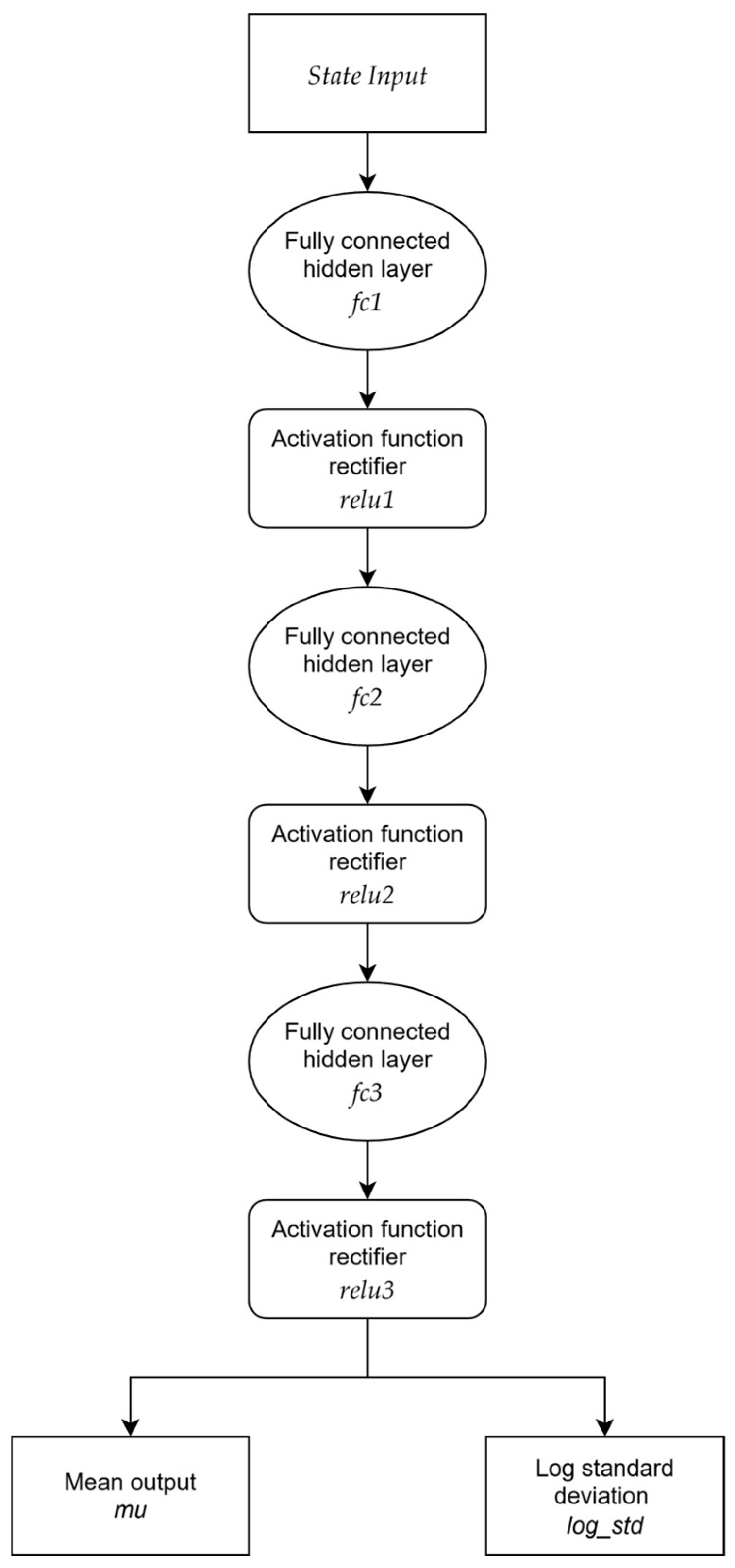
The network architectures in Figure 4a,b, which were used in the final version, were the result of the empirical testing of network performance. The actor network (a) contains an input layer denoted by input, three fully connected layers fc1, fc2 and fc3, 3 rectified linear unit activation functions relu1, relu2 and relu3, an output layer mu, followed by a final sigmoid activation function marked as sigma, which returns the action taken based on the input state.

The critic network architecture (b) is also fairly typical for DDPG and TD3 algorithms, where it receives double input vectors. The first input, denoted as State Input, is the state input followed by two fully connected layers—fc1 and fc2. Between them is a rectifier relu1. The action input path Action Input is only followed by a fully connected layer fc1_action. The outputs of fc2 and fc1_action (outputs must be same dimension) are summed elementwise in the summing step Sum. The summation is then passed into an activation function rectifier relu2, a fully connected layer fc3, another rectifier relu3, and finally into the final output layer q that returns the Q-value of the state-action pair. Following the basis of the TD3 algorithm, there are 2 critic networks. Both have the same architecture.

Hyperparameter tuning resulted in the following parameters, as shown in

Table 4. Hyperparameters used for DDPG and TD3.

Parameter	Value	Description
Actor learning rate	0.00004	Learning rate of the actor network
Critic learning rate	0.0004	Learning rate of the critic network
Discount factor	0.99	Discount factor for future rewards
Soft update factor	0.0002	Target network update rate
Replay buffer size	1,000,000	Size of the replay memory buffer
Hidden layer 1 (fc1) size	40	Number of neurons in the first hidden layer
Hidden layer 2 (fc2) size	40	Number of neurons in the second hidden layer
Hidden layer 3 (fc3) size	40	Number of neurons in the third hidden layer
Batch size	64	Size of mini batches used for training
Exploration noise	0.8	Added noise for action exploration
Exploration decay	0.999641	A selected decay of a Gaussian

. Tuning was performed using manual adjustments until satisfactory results were achieved.

To promote exploration during training, Gaussian noise was added to the actions output by the actor network. At each time step t, the exploration noise was sampled from a zero-mean normal distribution:

$$a_t= \mu \left(s_t\right)+\mathcal{N}\left(0,{\sigma }_t^2\right),$$

(19)

where $\mu \left(s_t\right)$ is the deterministic action predicted by the actor for state $s_t$, and ${\sigma }_t$ is the standard deviation of the noise at time step t. The noise scale was initialized at ${\sigma }_t=0.8$, and decayed exponentially over time as follows:

$${\sigma }_{t+1}= {\sigma }_t · \lambda ,$$

(20)

where $\lambda$ is the desired exploration decay. This ensures a high degree of exploration early in training and gradually reduces noise to help converge the policy to a stable level.

The SAC agent networks are very similar to TD3, with the exception that the actor in this case outputs the parameters of a stochastic policy [27]. In this case, it is presented in Figure 5 as two outputs per action dimension. The first is a state dependent mean ${\mu }_{\theta }\left(s_t\right)$, denoted in Figure 5 as mu, and the second is the logarithmic standard deviation $log{\sigma }_{\theta }\left(s\right)$, denoted in Figure 5 as log_std. Essentially, this is how SAC explores the state space. Actions are drawn via the re-parametrisation:

$$a_t={\mu }_{\theta }\left(s_t\right)+{\sigma }_{\theta }\left(s\right)· \epsilon$$

(21)

where $\epsilon$ is a vector of independent standard-normal noise serving two purposes:

• Re-parameterisation trick: By expressing the random action as a deterministic function of $\epsilon$, ${\mu }_{\theta }$, and ${\sigma }_{\theta }$, you can back-propagate gradients through the stochastic sampling step.
• State-dependent exploration: The spread is scaled by the learned ${\sigma }_{\theta }\left(s\right)$, so the policy controls how much noise is injected in each state.

We used a version PPO that uses the same stochastic policy actor as SAC. It also uses a very similar method of noise injection as Equation (21). The main differences between them come from objective and entropy treatment, variance parametrisation, and on-policy learning. PPO collects fresh trajectories each update and discards them, enforcing on-policy learning; SAC reuses experiences via a replay buffer, enabling higher sample efficiency [28].

Critic networks are the same as in TD3 and DDPG. Hyperparameters were once again tuned manually to achieve satisfactory results (hyperparameters of SAC and PPO are shown in

Table 5. Hyperparameters used for SAC.

Parameter	Value	Description
Actor learning rate	0.00001	Learning rate of the actor network
Critic learning rate	0.00005	Learning rate of the critic network
Discount factor	0.99	Discount factor for future rewards
Soft update factor	0.0004	Target network update rate
Replay buffer size	1,000,000	Size of the replay memory buffer
Hidden layer 1 (fc1) size	50	Number of neurons in the first hidden layer
Hidden layer 2 (fc2) size	50	Number of neurons in the second hidden layer
Hidden layer 3 (fc3) size	50	Number of neurons in the third hidden layer
Batch size	254	Size of mini batches used for training
Entropy weight	2	Entropy regularization scaling factor
Entropy weight learning rate	0.0003	Entropy weight parameter update step-size
Target entropy	0	Desired policy entropy threshold

and

Table 6. Hyperparameters used for PPO at the start of training.

Parameter	Value	Description
Actor learning rate	0.0005	Learning rate of the actor network
Critic learning rate	0.0008	Learning rate of the critic network
Discount factor	0.99	Discount factor for future rewards
Clip factor	0.12	Probability ratio clipping threshold
GAE factor	0.95	Advantage estimation bias-variance factor
Hidden layer 1 (fc1) size	50	Number of neurons in the first hidden layer
Hidden layer 2 (fc2) size	50	Number of neurons in the second hidden layer
Hidden layer 3 (fc3) size	50	Number of neurons in the third hidden layer
Batch size	548	Size of mini batches used for training
Experience horizon	10,405	Rollout length per policy update
Number of epochs	8	Policy optimization passes per batch
Entropy loss weight	0.02	Entropy bonus coefficient weight

).

Since PPO training is somewhat quicker and more stable, we kept retraining the PPO agent with different hyperparameters to fine tune it. Generally, we gradually reduced the entropy loss weight and clip factor, which improved the gained reward and even further stabilized training.

2.4. Human Dispatcher and Benchmark Method

The dispatcher in a hydropower plant plays a critical role in the real-time monitoring, coordination, and control of power generation and grid integration. While automation and Supervisory Control and Data Acquisition (SCADA) systems handle many operational tasks, the dispatcher ensures the safe, efficient, and optimized functioning of the power station within broader grid requirements. Our simplified RL agent is not designed to replicate all the dispatcher’s responsibilities, but to simply emulate the power generation decision-making step.

The publishing of the exact performance of a dispatcher is somewhat controversial, since the data is sensitive and could present a potential security risk. For this reason, we will simply focus on a generalized performance in terms of absolute mean error. Even though this does not represent the nuances of performance accuracy and its characteristics, it still shows the capabilities of the RL agent.

Specifically, we will compare the ability of the RL agent in reaching a general long-term load profile in 30 min steps and a historical real set-point reference in 15 min steps. In all tests, the goal is to minimize the absolute mean error and compare that to the generalized dispatcher’s tolerable absolute mean error of 5.8 MW. Since the dispatcher’s responsibilities as well as the capabilities far exceed the scope of the current RL agent, it is not expected to significantly improve the performance. This mainly results from the capability of the human dispatcher to make micro adjustments within the 15 min step, as well as more data availability.

The dispatchers must adhere to certain safety constraints in water level management. In most reservoirs of this model, the water level is only allowed to change the base water level from −1/−0.8 m to +0.2 m, except in the 7th reservoir where the river passes through a major metropolitan area and the water level is limited to −0.2 to +0.2 m. The water level change speed is limited in all reservoirs to 20 centimetres per hour.

3. Results

In the results, we will first analyze the performance of the RL agent on a generalized load reference profile in 30 min steps at the beginning of Chapter 3.1. This was done to test the capability of the RL agent by following simpler references. In the first experimental result, we could also analyze the error in the form of a percentage of the reference. That was done to obtain a better understanding of the performance. Unfortunately, the tests could not be repeated on real set-point data, since the reference commonly reaches 0 and the error calculation would then be a division by 0. For that reason, we will forgo the error percentage analysis.

In the latter part of Chapter 3, we try to match the RL agent’s performance to the performance of the human dispatcher on historical 15 min set-point reference and reservoir inflow data.

3.1. DDPG Training Results

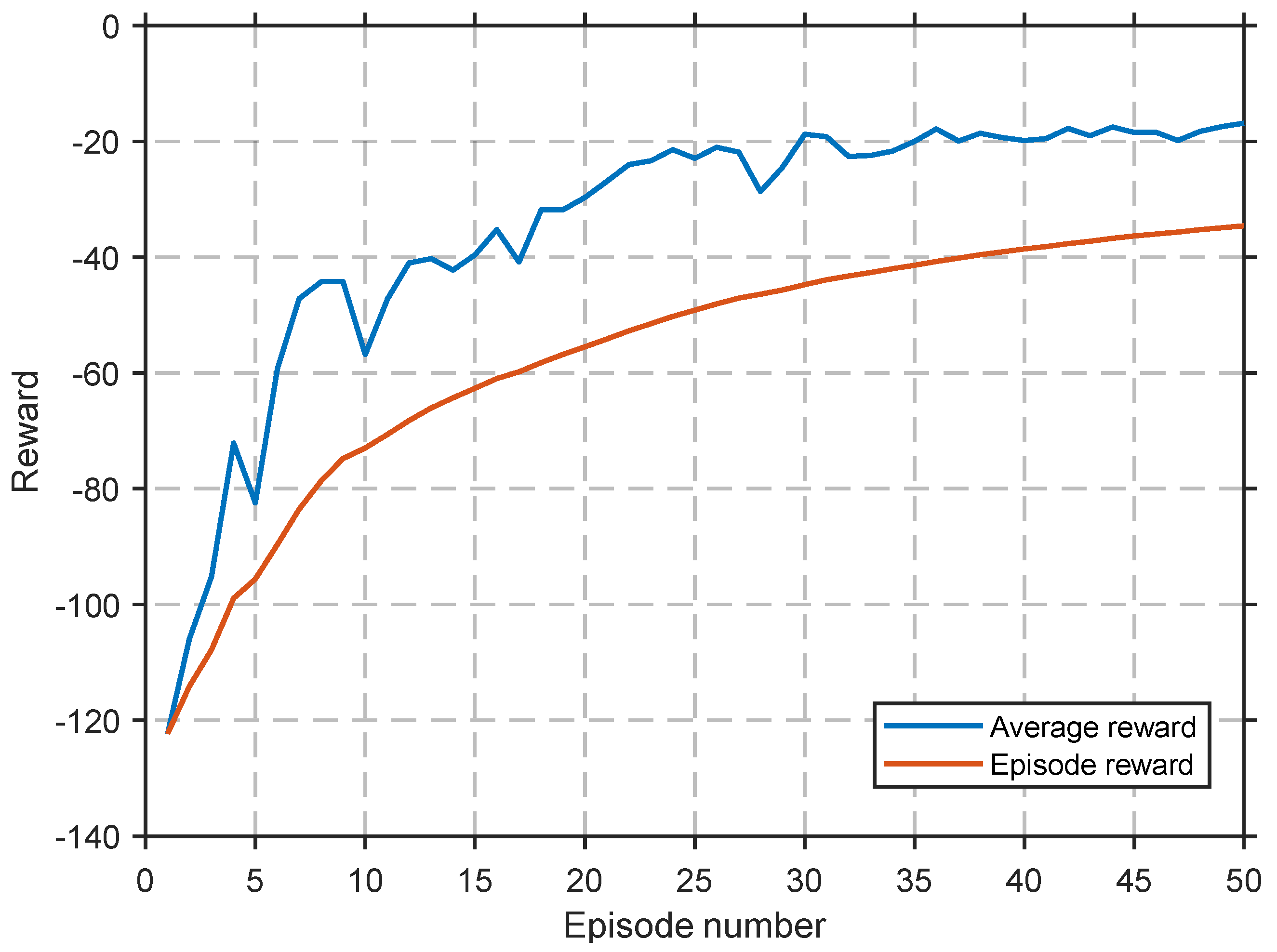
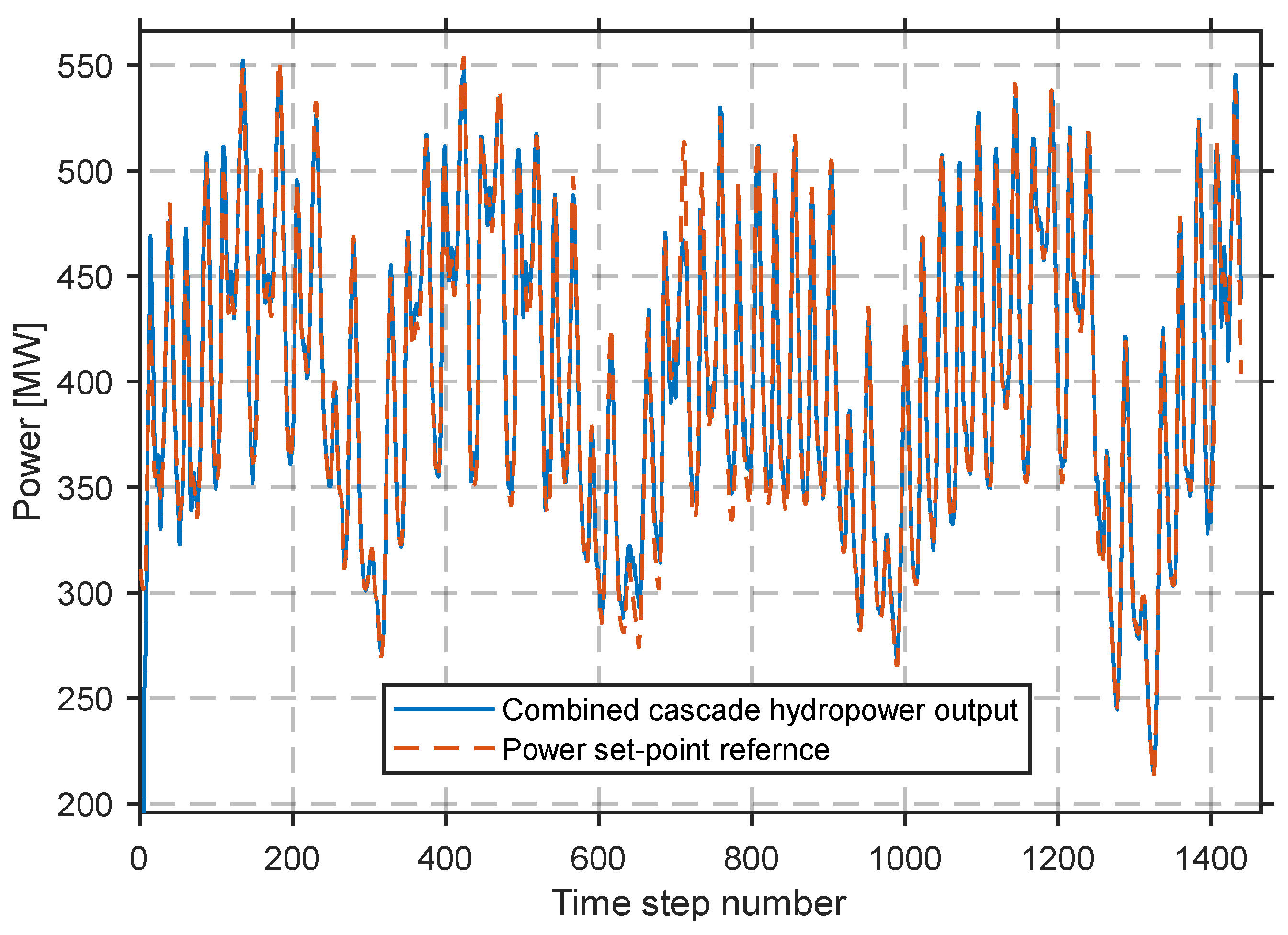
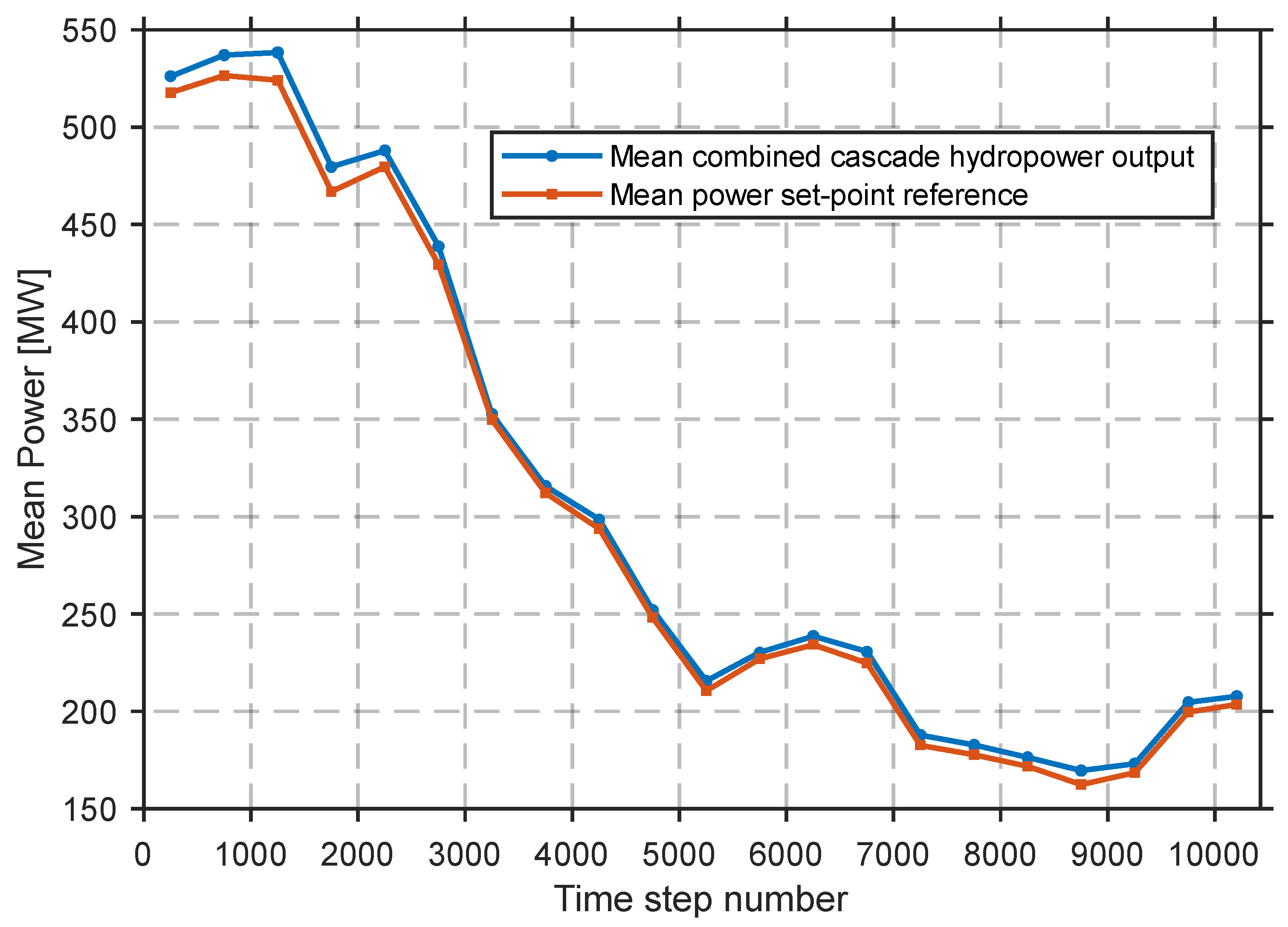
The first training iteration, shown in Figure 6, was performed on a reference signal that mirrors the power demand in Slovenia. This was done to show the ability of the RL agent to generalize the system dynamics and characteristics. In this case, we used 30 min time steps. All following time steps last 15 min.

We omit the initial sample (Time step number = 0) in Figure 7 and Figure 8 that shows a 100% tracking error. The episode was deliberately initialized with a large step to probe the agent’s transient response, and including that point would dominate the axis scale and obscure subsequent behaviour.

While the agent does not achieve perfect accuracy in set-point tracking, it demonstrates consistent performance across varying inflow conditions and avoids system instability. The agent achieves a mean absolute error of 6.38 MW. That deviation includes the beginning step response of the system starting at 0 power production with empty reservoirs. Importantly, large deviations and system instability were avoided.

Afterwards, we tested training on the 15 min real set-point data. We compare this 15 min data to the actions of a real dispatcher. The training was performed on the most recent reference data set.

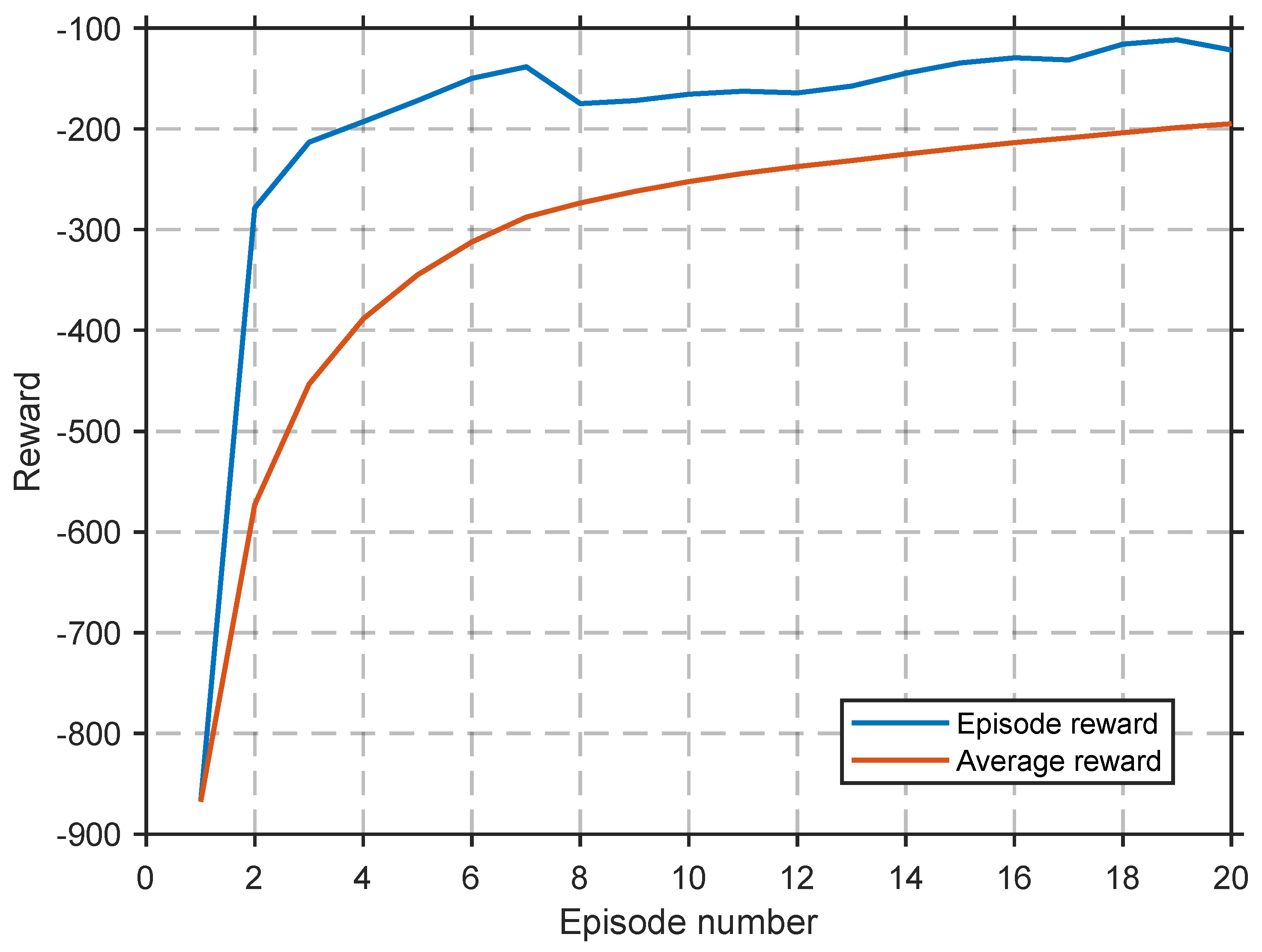
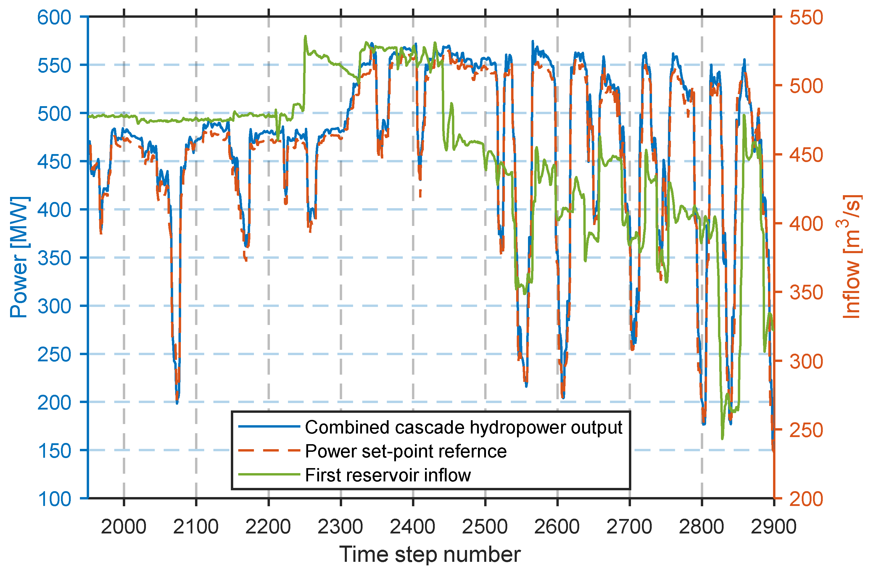
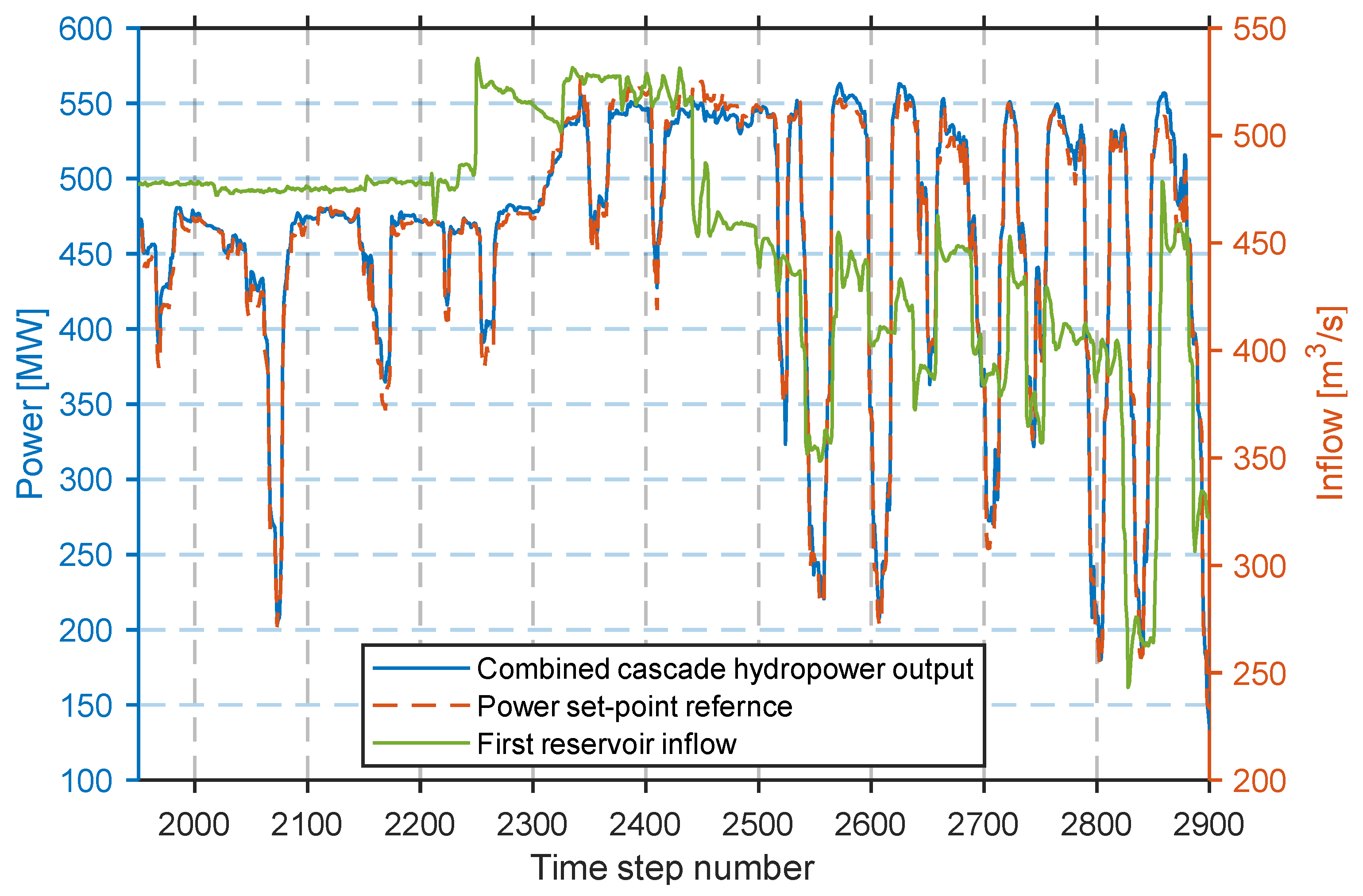
This time training the agent (Figure 9) achieved a mean absolute error of 11.93 MW (general error shown in Figure 10 and Figure 11). This was a downgrade in performance from the previous example in Figure 7. The reason for this could be more aggressive spikes in the set-point reference, which also include frequency restoration reserve demands. We can notice more discrepancies and errors, but generally, the decisions taken by the agent are relatively accurate and could be improved with further training. The training time for the agent was 5431.03 s.

3.2. TD3 Training Results

In training the TD3 agent (Figure 12), we directly started training on the real set-point data and dispatcher performance to gauge the possible improvement.

The agent achieves a mean absolute error of 7.64 MW (general error shown in Figure 13 and Figure 14). System instability was once again avoided, and large deviations did not occur. The training time for the agent was 5942.09 s.

3.3. SAC Training Results

The SAC training results (Figure 15) were very similar; however, due to its entropy-based exploration method, the agent did not fully settle during training and thus ended with a slightly higher final reward. During evaluation, when actions are deterministic, its performance is comparable to TD3 and DDPG (general performance shown in Figure 16 and Figure 17).

The agent achieves a mean absolute error of 9.06 MW. System instability was avoided. The training time for the agent was 6745.68 s.

3.4. PPO Training Results

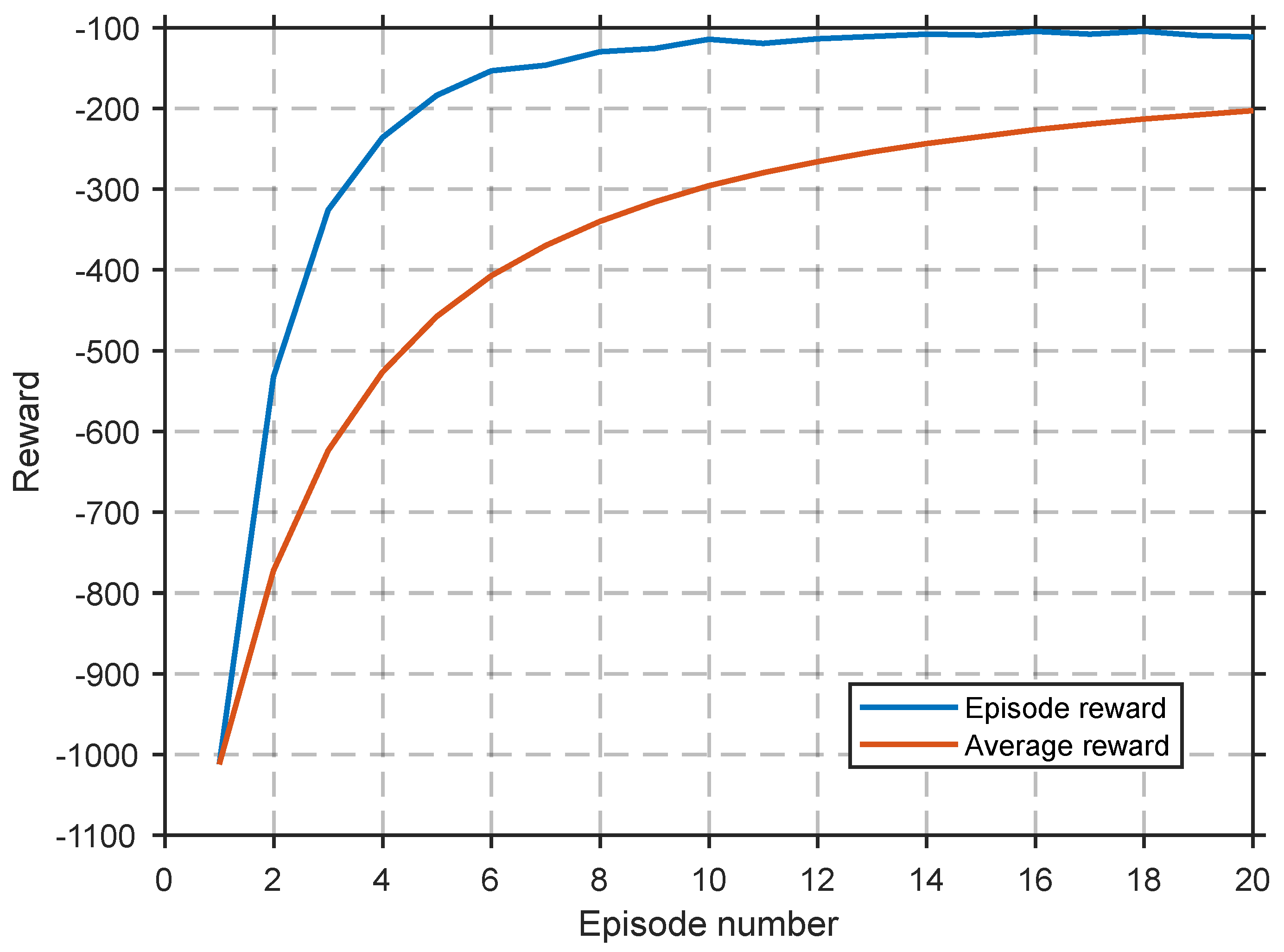
The initial training of PPO (Figure 18) shows a more gradual climb of episode rewards compared to DDPG, TD3 and SAC. The significantly faster training time of PPO due to it being an on-policy algorithm gives us more flexibility in hyperparameter tuning and agent retraining to achieve better performance. We also used many more training episodes than previously.

The agent achieves a mean absolute error of 8.81 MW. System instability was once again avoided, and large deviations did not occur. The training time for the agent was much shorter; however, we conducted multiple training iterations and tuning sessions.

3.5. Comparisons and Benchmarks

Across methods, all RL agents achieved satisfactory control precision. With additional hyperparameter tuning and modest network revisions, we think that the performance could approach, or potentially surpass, that of human dispatchers. PPO, which was comparatively easier to tune, produced the most stable tracking of the set-point trajectory (Figure 19 and Figure 20). Its higher absolute mean error appears to stem from a small steady-state bias, whereas TD3 exhibits lower steady-state error but larger transient deviations (“swing misses”). SAC also performed well overall; however, hyperparameter sensitivity—particularly to the entropy temperature setting—led to somewhat worse results than TD3 and PPO, though still better than DDPG. Among the tested methods, DDPG was the most training unstable (Figure 9). In Figure 21, we subtracted the mean power setpoint reference from each algorithm’s mean combined output for visual clarity. The small difference in performance is observable; this is apart from in DDPG, which exhibits a consistently higher error.

Given its consistency, we focus the discussion on TD3, which on average achieved slightly better results than DDPG, SAC, and PPO. That said, performance differences were not large across agents.

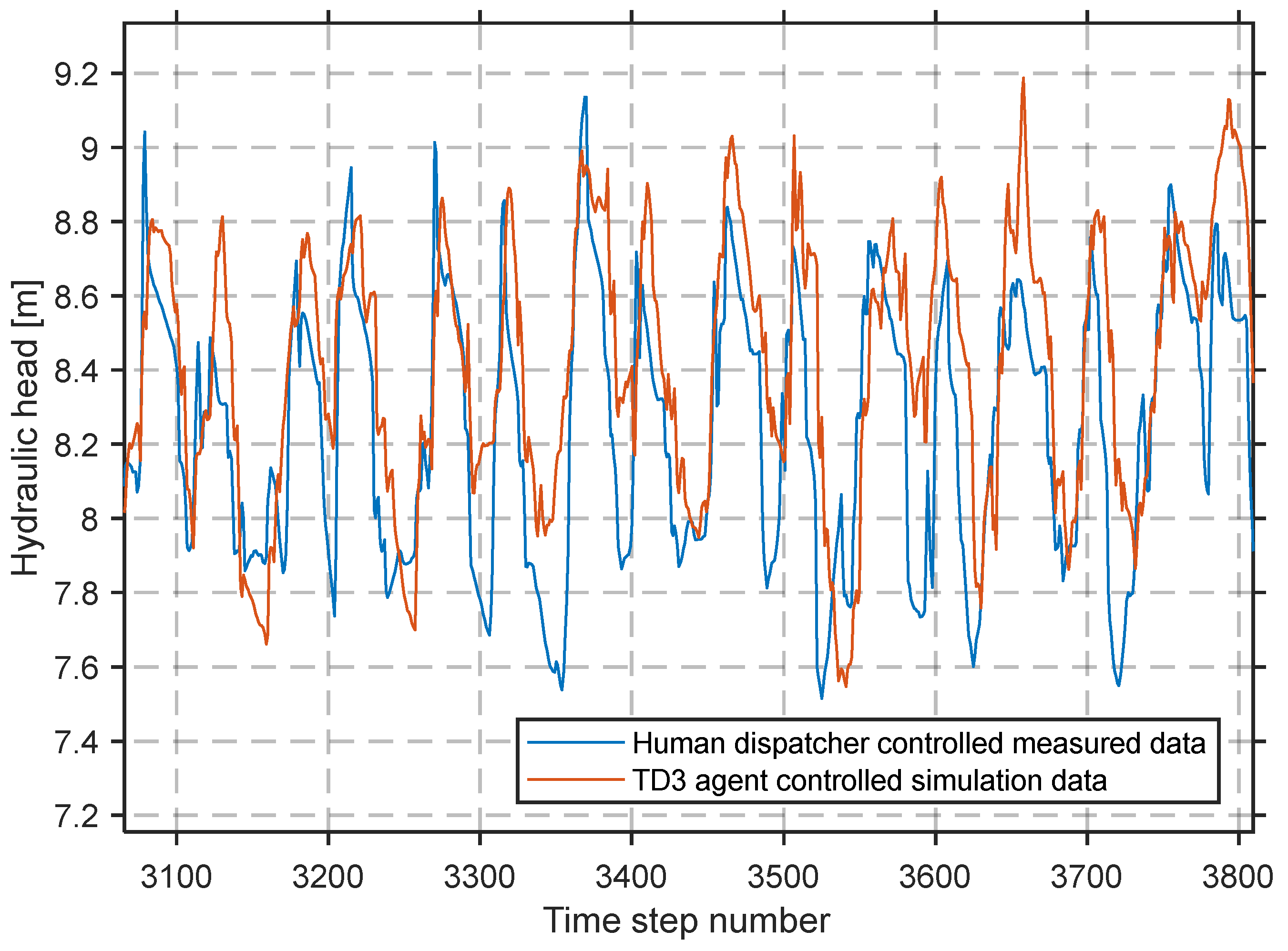
When benchmarked against human dispatchers, TD3 has not yet matched the same level of precision. Nevertheless, the control trajectories are qualitatively similar, as reflected in the hydraulic head profiles across plants (Figure 22 and Figure 23). These results partly validate both the digital-twin fidelity and the policy’s decision-making: residual discrepancies likely arise from model generalizations and unmodeled operational nuances, but the RL agent appears to converge toward human-like control decisions for cascade operation.

Compared with the previously discussed articles [11,12,16], article [12] benchmarked its approach against a simple “always-open” greedy policy and a mixed-integer linear-programming (MILP) model. As a result, the authors linearized their simulation model. Because the goal in [12] was to produce profit-seeking schedules under realistic constraints, their state representation included:

• Current and future natural inflows, which give the agent a look-ahead over a chosen horizon. In contrast, we treat original inflows as exogenous.
• Current and future energy prices: This is used to calculate system income.
• Subsystem metrics: Reservoir water volume, turbine flow, power production and number of active turbines. We essentially track very similar metrics in our state representation, except for the number of active turbines.
• Outflow discrepancies: The difference between the agent-chosen outflow and the realized outflow, which exposes the agent to system characteristics. In our work, this is captured implicitly: by including current plant power output in the state, the subsequent state transition informs the agent how its action changed power. These (state, next-state, action, reward) tuples form the basis of RL training.
• Outflow variations: Tracked to flag gate-movement constraint violations. Here, the benefit of a nonlinear formulation is evident, since we enforce hard constraints that the agent cannot violate, making this tracking redundant.
• Past outflows: Similar to our work, they model system delays by recording past outflows and use them as inputs for downstream reservoirs.

The reward function is centred around maximizing the total income $i_{d,t}$ per system d within the timestep t normalized within the market price $P_t$, with the added potential punishment for gate movement constrain violations indicated by $h_{d,t}$ and penalty H. This article also shows that simple reward functions work best with complex systems like hydropower plants [12].

$$r_t={\displaystyle \frac{{\sum }_{\mathrm{d}=1}^D(i_{d,t}-\mathrm{H}·h_{d,t})}{{max}_{t=1,\dots ,T}{ P}_t}}$$

(22)

Although similar to ours at quick glance, the reward function in Equation (22) differs fundamentally in how it guides the system. Its state representation looks ahead over a specified future horizon and optimizes the intraday production schedule, which positions the agent as a tool for traders and planners. Used in isolation, this is appropriate, since maximizing revenue via an optimal production profile is a valid objective. Our focus, however, is the case in which the cascade is embedded in a broader portfolio and the prescribed schedule may be suboptimal with respect to flows and system characteristics. Accordingly, our reward function ensures that the system handles exogenous inflows optimally, regardless of how traders constructed the production schedule.

Ref. [12]’s training curves also support our results, where PPO is the most stable in training; however, their system interaction differs between algorithms because they employ both continuous and discrete actions, and they use a special approach in which the agent optimizes a greedy policy. The time steps they used were the same as ours, 15 min.

Ref. [16] proposes a SAC agent for long-term hydropower scheduling, targeting yearly revenue under weekly inflow and price uncertainty. Rather than benchmarking against MILP or a greedy “always-open” baseline, they position RL as a complementary planner trained on stochastic variations in historical Nordic data; the simulation is deliberately simplified (single reservoir, linear production with respect to release, no cascades or pumps).

Their state representation includes:

• Week number, reservoir storage, weekly inflow, and weekly price: normalized to max storage/price to stabilize learning.
• “Weeks to empty at full capacity”: used to clamp the policy to feasible actions.

Regarding reward design, for a weekly action $a_t$, they use the following [16]:

$$r_t=a_t f_{max} r_{max}(y_{t }{k}_{price}{)}^{q_{price}}$$

(23)

where $f_{max}$ is the max production relative to storage capacity, $r_{max}$ is the reservoir volume and $y_{t }$ is the normalized weekly price; and $k_{price}$ and $q_{price}$ are tune price scaling and nonlinearity. They also add an end-of-year value-of-water term (rewarding terminal storage within a target band), but do not include penalties for gate-movement or ramping because such constraints are not needed in weeklong time steps. In contrast, this reward is fully tailored to the weekly time steps. Their episodes span 52 weeks with weekly decision steps; the agent is trained for in the order of $3 · {10}^5$ episodes on stochastic scenarios assembled from NO3 price data (2008–2019) and long-history inflows combined from four Norwegian reservoirs. Our studies operate at 15 min granularity and target cascaded plant behaviour under more detailed operational constraints, making the direct comparison of policies and stability less like-for-like.

The main reason we closely reviewed this study is their employment SAC, which explicitly handles continuous actions and encourages exploration in stochastic regimes, which is also useful for our system. Their learning curves show sensible convergence to a policy that releases more during high-price periods while maintaining terminal storage, and they emphasize that RL should complement, not replace, traditional optimization.

The study [16] validates SAC on a simplified, single-reservoir, weekly scheduling problem with normalized price/inflow states and a price-weighted production reward plus terminal storage value. Our work addresses a more granular, constrained, and cascaded setting; we enforce hard constraints directly and design rewards to ensure robust operation under exogenous inflows irrespective of trader-specified schedules.

They do not however explicitly compare their results to any benchmark or method. The paper trains a SAC agent and presents learning curves and example weekly policies on artificial and historical scenarios, framing RL as a complementary tool rather than a replacement and offering no head-to-head quantitative comparison to classical schedulers.

The final compared study [11] evaluates four policy-gradient DRL methods—DDPG, TD3, SAC18, SAC19—on a single-reservoir problem with comparisons against Standard Operating Policy (SOP) and historical “base” operation. The physical model enforces flood-control and hydraulic constraints. The state is intentionally compact. It contains normalized storage and a cyclic month encoding (two sin/cos components), yielding a 3-D state vector. No prices or cascade interactions enter the state.

Per time step, the reward balances hydropower generation against the squared water-supply deficit, with an added penalty for unsafe spills [11]:

$$r_t={GP}_t- D_t^2+ P_t$$

(24)

where ${GP}_t$ is the power produced, $D_t^2$ is the deficit and $P_t$ is the penalty (negative) for deviation from the system requirements. This favours meeting demand and producing energy while heavily discouraging flood-risk exceedances. Generally, this is very similar to our reward function. The main differences are the flood-risk penalty and time step handling, where decisions are made monthly. Demand signal following as a concept is closer to trader-imposed schedules; however, significant differences can occur, especially in larger water management or energy portfolios.

We bridged the gaps between these studies [6,11,12] and provided a concise control method which combines the fine-grained control of [12] and the general operational style of [11,16], while adding an additional perspective on the differences between schedulers and dispatchers.

4. Discussion

The results demonstrate that a model-free RL agent can approach the performance of an expert human dispatcher in real-time cascade control. Our TD3 controller achieved an absolute mean power tracking error of 7.64 MW (about 1.3% of the 592 MW capacity) with zero constraint violations, compared to 5.8 MW (≈1.0%) and over 14,000 minor violations for the human operator (

Table 7. Result recapitulation.

Method	Time Step	Absolute Mean Error	Safety Constraint Violations
Human dispatcher	Real time	5.8 MW	14,121
DDPG	30 min/15 min	6.38 MW/11.93 MW	0
TD3	15 min	7.64 MW	0
SAC	15 min	9.06 MW	0
PPO	15 min	8.81 MW	0

). Previous studies on hydropower RL have largely focused on scheduling problems or simplified settings, such as optimizing day-ahead generation plans or single-reservoir operations [9,10], rather than the real-time dispatch of a full cascade under stochastic inputs. By filling this gap, our work extends recent findings on RL’s potential in water systems into the operational domain, showing that an agent can make decisions that mimic a dispatcher’s actions in a live cascade.

Numerous prior efforts have applied RL or other AI techniques to hydropower management, but under different objectives and assumptions. For example, ref. [12] similarly investigated continuous-action RL (SAC, PPO, A2C) for intraday economic optimization of a multi-reservoir system, aiming to maximize profit under complex constraints (e.g., turbine ramping limits and time-of-use electricity prices). Those studies confirm that RL can learn efficient operating policies for hydropower; however, they still treat the problem as an optimization of generation or revenue over a horizon, rather than tracking an externally imposed schedule in real time. In contrast, our agent is tasked with following a given power trajectory set by market operators, a scenario much closer to actual dispatcher duties. This distinction is crucial; our work demonstrates that even when the “optimal” schedule is exogenously defined (and possibly infeasible), an RL controller can intelligently adjust flows to minimize deviations, essentially serving as a digital dispatcher. To our knowledge, no previous RL study on cascades [8,9,10,11,12,13,14,15,16,17,18,19,20,21] has directly benchmarked against human operators in such a real-time tracking context, underscoring the novelty of our contribution.

In terms of absolute performance, the RL agent’s tracking error falls within ~2 MW of the human dispatcher on average, which is a remarkably small gap considering the agent had no direct knowledge of inflow or market forecasts. This result aligns with Sadeghi Tabas and Samadi’s recent findings that advanced policy-gradient agents (TD3, SAC) can reliably meet operational targets in single-reservoir control [11]. In our case, the RL policy not only met power targets nearly as well as an expert, but did so without violating any operational constraints, whereas human controllers logged 1785 water-level and 12,336 down-ramping violations over the same period. A similar benefit was noted by [14], who introduced chance-constraint “backoffs” into an RL algorithm to reduce the risk of spills in a multi-reservoir system; their approach traded a modest 1.5% of generation output for substantially fewer overflow events. Our agent achieved a comparable outcome (zero spills) naturally through hard-coded constraints, sacrificing a small amount of precision in hitting the exact set-point in exchange for enhanced safety. We observe that human dispatchers, by contrast, occasionally intentionally in minor amounts violated constraints (e.g., temporarily exceeding a maximum level or ramp rate) to better track the schedule. This discretionary freedom gave the humans a slight edge in accuracy, but at the cost of rule compliance. Such behaviour underscores a fundamental trade-off between performance and safety that dispatchers navigate. The RL agent, constrained by design to never break rules, essentially chose the safer side of that trade-off. In practice, these minor violations by humans did not cause damage (they were usually within a few percent of limits and often due to unmodeled dynamics like seiches), but they hint at why the agent’s error could not match the absolute best human performance. Overall, considering the strict constraint observance, the agent’s error is on par with the performance achieved in far simpler settings (e.g., [11]), reinforcing that our RL approach maintains high performance without the need to relax operating limits.

A key factor in the agent’s success is the high-fidelity data-driven simulation model environment used for training. We modelled all eight plants with realistic water travel delays, nonlinear turbine curves, and inter-reservoir dynamics, using 15 min time steps to capture the system’s fast response. It is worth noting that [13] recently highlighted the importance of high-fidelity simulation for RL in safety-critical energy systems, demonstrating a digital twin-based RL for a pumped-storage plant startup procedure.

While the proposed RL framework shows strong performance, several limitations must be acknowledged in the context of both our work and related studies. First, the agent’s decisions are currently made at a fixed 15 min interval and tested in a simulated environment. This discrete decision was chosen to match the market schedule granularity and reflects a balance between operational detail and training complexity. Human dispatchers continuously monitor and can fine-tune outputs almost instantaneously if needed. Our 15 min agent cannot make sub-interval adjustments, which means it may miss some opportunities for correction within each interval. A possible improvement, suggested by the paradigm of model-predictive control or high-frequency RL, is to enable more frequent decision-making or hierarchical control where the RL sets targets that lower-level traditional controller’s track. Second, our digital twin, while comprehensive, is not perfect. We assumed constant minor inflows (torrential tributaries) and neglected certain hydrodynamic phenomena (e.g., fast water surface oscillations or seiches). These unmodeled factors likely explain many of the minor level-rate violations observed in the real system—for instance, the 7th reservoir (through a city area) showed frequent tiny fluctuations beyond the 5 cm/15 min limit, which the simulator did not reproduce. Incorporating such effects would require either higher-fidelity physics or data-driven adjustments (e.g., disturbance models), which could be an area of future enhancement. Third, the agent’s generalization beyond the training distribution is unproven. Truly unseen conditions (a record flood, an unprecedented market spike, etc.) were not part of this evaluation.

Future Work and Application

Following the creation of an RL agent that can control the cascade hydropower plant similarly to a human dispatcher, we can integrate it into a wider digital twin model of the entire portfolio of Slovenian energy production. Considering the RL agent as a good estimate of dispatcher decision-making, we can analyze the changes in the operation of the cascade with a changing production schedule that contains the rising concern of negative energy pricing on European energy markets. Its main goal is to have a solid gauge of the available flexibility of the system.

5. Conclusions

We built a high-fidelity, data-driven digital twin of the eight-plant Drava cascade and trained model-free RL controllers (DDPG, TD3, SAC, PPO) for real-time tracking of trader-set schedules. The best agent (TD3) achieved a mean absolute tracking error of 7.64 MW with zero safety/operational violations, approaching human dispatcher performance (5.8 MW) while eliminating 1785 water-level and 12,336 ramp-rate violations. Our contributions are: a real-time RL formulation under exogenous schedules, a digital twin capturing nonlinear head–flow coupling, and a head-to-head benchmark against expert dispatchers. Limitations include simplified tributary inflows, the omission of seiche-scale hydrodynamics, a fixed 15 min decision interval, and evaluation in simulation. Future work will couple the controller with upstream scheduling, refine the hydraulic model, explore hierarchical/multi-agent control, and study human–AI collaboration for safe deployment.

References

1. Statistical Office of the Republic of Slovenia. Energy. SiStat Database. Available online: https://pxweb.stat.si/SiStat/en/Podrocja/index/186/energy#243 (accessed on 28 July 2025).
2. Dravske elektrarne Maribor d.o.o. (DEM d.o.o.). Available online: https://www.dem.si/en/ (accessed on 28 July 2025).
3. Hamann, A.; Hug, G. Real-time optimization of a hydropower cascade using a linear modeling approach. In Proceedings of the 18th Power Systems Computation Conference (PSCC 2014), Wroclaw, Poland, 18–22 August 2014; IEEE: Piscataway, NJ, USA, 2014; pp. 1–7. [Google Scholar] [CrossRef]
4. Catalao, J.P.S.; Mariano, S.J.P.; Mendes, V.M.F.; Ferreira, L.A.F. Scheduling of Head-Sensitive Cascaded Hydro Systems: A Nonlinear Approach. IEEE Trans. Power Syst. 2009, 24, 337–346. [Google Scholar] [CrossRef]
5. Arce, A.; Ohishi, T.; Soares, S. Optimal dispatch of generating units of the Itaipu hydroelectric plant. IEEE Trans. Power Syst. 2002, 17, 154–158. [Google Scholar] [CrossRef]
6. Resman, M.; Protner, J.; Simic, M.; Herakovic, N. A Five-Step Approach to Planning Data-Driven Digital Twins for Discrete Manufacturing Systems. Appl. Sci. 2021, 11, 3639. [Google Scholar] [CrossRef]
7. Faria, R.d.R.; Capron, B.D.O.; Secchi, A.R.; de Souza, M.B., Jr. Where Reinforcement Learning Meets Process Control: Review and Guidelines. Processes 2022, 10, 2311. [Google Scholar] [CrossRef]
8. Wu, Y.; Su, C.; Liu, S.; Guo, H.; Sun, Y.; Jiang, Y.; Shao, Q. Optimal Decomposition for the Monthly Contracted Electricity of Cascade Hydropower Plants Considering the Bidding Space in the Day-Ahead Spot Market. Water 2022, 14, 2347. [Google Scholar] [CrossRef]
9. Xu, W.; Yin, X.; Zhang, C.; Li, Z. Deep Reinforcement Learning for Cascaded Hydropower Reservoirs Considering Inflow Forecasts. Water Resour. Manag. 2020, 34, 3003–3018. [Google Scholar] [CrossRef]
10. Xu, W.; Yin, X.; Li, Z.; Yu, L. Deep Reinforcement Learning for Optimal Hydropower Reservoir Operation. J. Water Resour. Plan. Manag. 2021, 147, 04021045. [Google Scholar] [CrossRef]
11. Sadeghi Tabas, S.; Samadi, V. Fill-and-Spill: Deep Reinforcement Learning Policy Gradient Methods for Reservoir Operation Decision and Control. J. Water Resour. Plan. Manag. 2024, 150, 04023034. [Google Scholar] [CrossRef]
12. Castro-Freibott, R.; Pereira, M.; Rosa, J.; Pérez-Díaz, J. Deep Reinforcement Learning for Intraday Multireservoir Hydropower Management. Mathematics 2025, 13, 151. [Google Scholar] [CrossRef]
13. Tubeuf, C.; Bousquet, Y.; Guillaud, X.; Panciatici, P. Increasing the Flexibility of Hydropower with Reinforcement Learning on a Digital Twin Platform. Energies 2023, 16, 1796. [Google Scholar] [CrossRef]
14. Mitjana, F.; Ostfeld, A.; Housh, M. Managing Chance-Constrained Hydropower with Reinforcement Learning and Backoffs. Adv. Water Resour. 2022, 163, 104308. [Google Scholar] [CrossRef]
15. Castelletti, A.; Galelli, S.; Restelli, M.; Soncini-Sessa, R. Tree-Based Reinforcement Learning for Optimal Water Reservoir Operation. Water Resour. Res 2010, 46, W09507. [Google Scholar] [CrossRef]
16. Riemer-Sørensen, S.; Rosenlund, G.H. Deep Reinforcement Learning for Long Term Hydropower Production Scheduling. arXiv 2020, arXiv:2012.06312. [Google Scholar] [CrossRef]
17. Li, X.; Ma, H.; Chen, S.; Xu, Y.; Zeng, X. Improved Reinforcement Learning for Multi-Objective Optimization Operation of Cascade Reservoir System Based on Monotonic Property. Water 2025, 17, 1681. [Google Scholar] [CrossRef]
18. Lee, S.; Labadie, J.W. Stochastic Optimization of Multireservoir Systems via Reinforcement Learning. Water Resour. Res. 2007, 43, W11408. [Google Scholar] [CrossRef]
19. Ma, X.; Pan, H.; Zheng, Y.; Hang, C.; Wu, X.; Li, L. Short-Term Optimal Scheduling of Pumped-Storage Units via DDPG with AOS-LSTM Flow-Curve Fitting. Water 2025, 17, 1842. [Google Scholar] [CrossRef]
20. Rani, D.; Moreira, M.M. Simulation–Optimization Modeling: A Survey and Potential Application in Reservoir Systems Operation. Water Resour. Manag. 2010, 24, 1107–1138. [Google Scholar] [CrossRef]
21. Xie, M.; Liu, X.; Cai, H.; Wu, D.; Xu, Y. Research on Typical Market Mode of Regulating Hydropower Stations Participating in Spot Market. Water 2025, 17, 1288. [Google Scholar] [CrossRef]
22. Bernardes, J., Jr.; Santos, M.; Abreu, T.; Prado, L., Jr.; Miranda, D.; Julio, R.; Viana, P.; Fonseca, M.; Bortoni, E.; Bastos, G.S. Hydropower Operation Optimization Using Machine Learning: A Systematic Review. AI 2022, 3, 78–99. [Google Scholar] [CrossRef]
23. Brezovnik, R. Short Term Optimization of Drava River Hydro Power Plants Operation. Bachelor’s Thesis, University of Maribor, Maribor, Slovenia, 2009. Available online: https://dk.um.si/IzpisGradiva.php?id=9862 (accessed on 2 July 2025).
24. Brezovnik, R.; Polajžer, B.; Grčar, B.; Popović, J. Development of a Mathematical Model of a Hydropower-Plant Cascade and Analysis of Production and Power Planning on DEM and SENG: Study Report; Available Upon Request with the Corresponding Author; UM FERI: Maribor, Slovenia, 2011. [Google Scholar]
25. Lillicrap, T.P.; Hunt, J.J.; Pritzel, A.; Heess, N.; Erez, T.; Tassa, Y.; Silver, D.; Wierstra, D. Continuous Control with Deep Reinforcement Learning. arXiv 2015, arXiv:1509.02971. [Google Scholar] [CrossRef]
26. Fujimoto, S.; Hoof, H.; Meger, D. Addressing Function Approximation Error in Actor-Critic Methods. arXiv 2018, arXiv:1802.09477. [Google Scholar] [CrossRef]
27. Haarnoja, T.; Zhou, A.; Abbeel, P.; Levine, S. Soft actor-critic: Off-policy maximum entropy deep reinforcement learning with a stochastic actor. arXiv 2018, arXiv:1801.01290. [Google Scholar] [CrossRef]
28. Schulman, J.; Wolski, F.; Dhariwal, P.; Radford, A.; Klimov, O. Proximal Policy Optimization Algorithms. arXiv 2017, arXiv:1707.06347. [Google Scholar] [CrossRef]
Figure 1. Sketch map of the Drava River system and hydropower plant locations.
Energies 18 04660 g001
Figure 2. Example of data fitting of the tailwater level with integrated MATLAB functions.
Energies 18 04660 g002
Figure 3. An example of data fitting of power production using integrated MATLAB functions.
Energies 18 04660 g003
Figure 4. (a) NN architecture of the actor; (b) NN architecture of the critic.
Energies 18 04660 g004
Figure 5. SAC and PPO actor network architecture.
Energies 18 04660 g005
Figure 6. DDPG training rewards graph on generalized power demand reference.
Energies 18 04660 g006
Figure 7. DDPG agent generalized load profile signal following.
Energies 18 04660 g007
Figure 8. Error percentage of the DDPG agent signal following.
Energies 18 04660 g008
Figure 9. DDPG training rewards graph on real set-point data.
Energies 18 04660 g009
Figure 10. Difference between mean power set-point and DDPG controlled output.
Energies 18 04660 g010
Figure 11. An arbitrary close-up of the results of the DDPG agent performance.
Energies 18 04660 g011
Figure 12. The TD3 agent rewards on real set-point data.
Energies 18 04660 g012
Figure 13. Difference between mean power set-point and TD3 controlled output.
Energies 18 04660 g013
Figure 14. An arbitrary close-up of the results of the TD3 agent performance.
Energies 18 04660 g014
Figure 15. The SAC agent rewards on real set-point data.
Energies 18 04660 g015
Figure 16. Difference between mean power set-point and SAC controlled output.
Energies 18 04660 g016
Figure 17. An arbitrary close-up of the results of the SAC agent performance.
Energies 18 04660 g017
Figure 18. Initial training PPO agent rewards on real set-point data.
Energies 18 04660 g018
Figure 19. Difference between mean power set-point and PPO controlled output.
Energies 18 04660 g019
Figure 20. An arbitrary close-up of the results of the PPO agent performance.
Energies 18 04660 g020
Figure 21. Set-point reference subtracted from all algorithm’s mean combined output.
Energies 18 04660 g021
Figure 22. Hydraulic head for the first power plant in the cascade.
Energies 18 04660 g022
Figure 23. Close-up of Figure 22.
Energies 18 04660 g023