Abstract
This study proposes a current control strategy to enhance the control stability of an interior permanent magnet synchronous motor (IPMSM) under transient conditions, such as rapid acceleration or deceleration in electric vehicle (EV) applications. Conventional current control methods provide optimal steady-state current references corresponding to torque commands using a lookup table (LUT)-based approach. However, during transitions between these reference points, particularly in the field-weakening region at high speeds, the voltage limit may be exceeded. When the voltage limit is exceeded, unstable overmodulation states may occur, degrading stability and resulting in overshoot of the inverter input current. Although ramp generators are commonly employed to interpolate between current references, a fixed ramp slope may fail to ensure a sufficient voltage margin during rapid transients. In this study, a method is proposed to dynamically adjust the rate of change of the d-axis current reference in real time based on the difference between the inverter output voltage and its voltage limit. By enabling timely field-weakening before rapid changes in speed or q-axis current, the proposed strategy maintains control stability within the voltage limit. The effectiveness of the proposed method was verified through simulations based on real vehicle driving profiles and dynamometer experiments using a 38 kW class IPMSM for a hybrid electric vehicle (HEV), demonstrating reduced input DC current overshoot, improved voltage stability, and enhanced torque tracking performance under high-speed transient conditions.
1. Introduction
IPMSMs used in xEVs have been widely adopted as key components of drive systems due to their high power density, excellent efficiency, and precise torque control capability over a wide speed range [1,2,3,4]. IPMSMs are capable of delivering maximum torque below the base speed. Above the base speed, field-weakening control enables high-speed operation within the voltage limit of the inverter [5,6]. Accordingly, the use of IPMSMs is expanding not only in EV drive systems but also in various industrial applications where high performance is required [7]. In the actual driving environments of EVs, frequent acceleration and deceleration occur in both urban and highway conditions. Accordingly, the motor is required to operate not only under steady-state conditions but also in response to varying speeds and dynamic load changes [8]. To reflect these actual driving conditions, motor evaluations are conducted not only under typical steady-state operations but also using various speed–torque driving profiles. Figure 1 shows an example of a speed–torque profile that simulates real EV driving conditions. As observed in the graph, transient regions with rapid changes in both speed and torque frequently appear within a short time frame. In such regions, the motor voltage and current can change abruptly. These profile-based tests, which reflect actual driving conditions, serve as an essential basis for comprehensively evaluating the transient response and control stability of motor control systems [9].
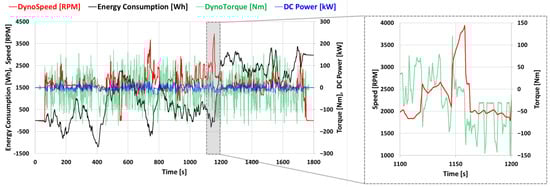
Figure 1.
Motor speed–torque profile in xEV driving conditions.
Accordingly, in EV drive systems, accurate torque response and high control stability are required over the entire driving range under various torque and speed conditions [10]. To achieve such control performance, optimal d-axis and q-axis current references corresponding to given torque commands are commonly derived through prior experiments under various conditions and stored in an LUT. The LUT, which contains current references mapped to torque and flux conditions, extracts optimal current references in real time based on the torque command from the vehicle control unit, the current motor speed, and the DC-link voltage. These current references are then provided to the current controller to ultimately generate the desired torque output [11].
However, if the current reference extracted from the LUT is applied directly to the current controller, the controller’s fast response may cause the torque to rise too rapidly, resulting in excessive mechanical stress on the drivetrain. For example, when a large torque command is applied instantaneously, the resulting rapid torque response may cause tire slip or lead to abrupt torque transmission, which can degrade ride comfort and impair driving stability [12]. For this reason, the current reference is not directly applied to the current controller. Instead, a ramp generator is used to gradually increase or decrease the current reference at a fixed rate during each control cycle. This approach enables modulation of the current response rate, allowing smooth control that accounts for both the dynamic characteristics of the vehicle and mechanical durability. Accordingly, the ramp slope of the current reference is predefined based on the characteristics of the vehicle type or drivetrain system, allowing both adequate responsiveness and ride comfort to be achieved simultaneously [13].
However, from the perspective of motor control, if the ramp slope of the current reference is fixed, the inverter output voltage may exceed the voltage limit during transient operating conditions in which the motor state changes rapidly, such as during rapid acceleration or deceleration. In such cases, the inverter enters the overmodulation region, which is a nonlinear control area, resulting in degraded control stability of the current controller [14,15,16,17]. Accordingly, this paper proposes a control strategy to address this issue by dynamically adjusting the rate of change of the current reference inside the ramp generator in real time, based on the voltage margin defined as the difference between the inverter output voltage and the voltage limit. In particular, since the q-axis current directly affects the torque, its ramp slope is kept constant to maintain the required responsiveness of the drive system. Meanwhile, the rate of change of the d-axis current is adjusted to ensure a sufficient voltage margin, thereby achieving stable current control. This control strategy causes the d-axis current response to either advance or delay during transient conditions, thereby counteracting voltage rises caused by speed or q-axis current. As a result, the controller can operate stably without exceeding the voltage limitation region.
The proposed method was validated using a dynamometer test setup based on a 38 kW class IPMSM and an inverter designed for HEV specifications. In addition, performance comparisons with the conventional control method were conducted using four speed–torque profiles that emulate various real driving modes. The experimental results confirmed significant improvements in both output torque accuracy and DC energy consumption during transient conditions in high-speed driving scenarios. These findings indicate that the proposed strategy can contribute to improved control reliability and extended driving range in xEV drive systems.
2. Conventional Control Structure and Challenges in Transient States
An IPMSM-based xEV drive system must perform precise current control in response to the torque command from the vehicle control unit, which varies in real time. To achieve this, a current reference is typically generated using an LUT based on the torque and flux commands. The torque–current LUT is constructed based on experimental data obtained under various operating conditions. It stores the optimal d-axis and q-axis current references corresponding to each combination of torque command, motor speed, and DC-link voltage in a tabulated form. Using this LUT, the appropriate current references are retrieved according to real-time operating conditions, enabling optimal control performance. Figure 2 illustrates a typical controller structure of an IPMSM used in an xEV drive system.
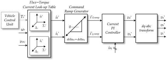
Figure 2.
Conventional IPMSM controller structure for xEV applications.
The torque command Te* received from the vehicle controller is converted into the d-axis and q-axis current commands, id* and iq*, through a pre-established LUT based on the motor speed ωr and the battery voltage vDC. The generated current commands are not directly applied to the controller; instead, they are processed by a ramp generator to impose constant rates of change, deltaid and deltaiq, resulting in the ramped current commands id*ramp and iq*ramp. The current controller calculates the reference voltages vd* and vq* to be applied to the inverter using individual PI controllers based on the d-axis and q-axis current errors. These voltages are then transformed into the three-phase voltage commands va*, vb* and vc* via inverse dq-to-abc transformation. Based on the generated phase voltage commands, the inverter determines the switching duties to supply the required currents to the motor, thereby ensuring that the target torque is accurately tracked. This controller structure is designed based on stable control performance under steady-state conditions and incorporates a ramp generator to regulate the response speed between current reference points. To prevent abrupt torque responses, the ramp generator does not apply the target current reference obtained from the LUT directly to the current controller. Instead, it gradually adjusts the reference at a fixed slope in each control cycle.
As shown in Equations (1) and (2), the ramp generator gradually increases or decreases the current reference by deltaid and deltaiq at each control cycle until the final target values id* and iq*, obtained from the LUT, are reached. During this process, the ramped current references id*ramp and iq*ramp are applied to the current controller. This mechanism allows the overall drive system responsiveness to be adjusted, playing a key role in maintaining a balance between driving stability and ride comfort by preventing physical disturbances caused by sudden torque changes. Therefore, it is important to predefine the ramp slope according to the characteristics of the drive system and apply it to the controller.
The operating region of an IPMSM applied to xEVs is generally defined by two physical constraints. The first is the maximum current, determined by the thermal rating of the motor windings and the cooling capability, as expressed in (3). The second is the maximum output voltage, determined by the applied DC-link voltage and the pulse width modulation (PWM) method, as expressed in (4).
In this context, the voltage equation of the IPMSM is given in (5), where R denotes the stator winding resistance, Ld and Lq represent the d-axis and q-axis inductances, respectively, ψf is the flux produced by the permanent magnets, and ω is the electrical angular velocity. Considering that the voltage drop caused by the winding resistance R is negligible compared with the electromotive force components determined by Ld and Lq, and assuming a steady-state conditions without abrupt current variations, (5) can be simplified to (6).
By substituting (6) into the voltage limit Equation (4) and simplifying, (7) is obtained. These conditions can be represented in the current synchronous reference frame as a current limit circle and a voltage limit ellipse, as shown in Figure 3. In particular, the center of the voltage ellipse is located in the negative d-axis direction by ψf/Ld, and its size decreases as the motor speed increases, thereby reducing the available operating region. Consequently, the operating region of the IPMSM must lie within the intersection of the current limit circle and the voltage limit ellipse, and the available voltage margin decreases sharply in the high-speed region.
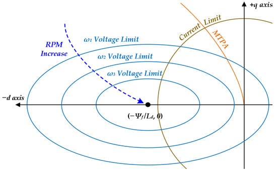
Figure 3.
Current limit circle and voltage limit ellipse of an IPMSM.
In conventional IPMSM control structures, the ramp slopes of the d-axis and q-axis current commands are typically set to be identical, allowing the current commands to change gradually. However, in actual operating conditions, transient events such as rapid acceleration or deceleration occur frequently. Under such conditions, a fixed ramp slope may fail to account for the physical constraints of the system, potentially leading to control instability. Figure 4 illustrates this issue by showing, step by step, how the current commands in the d–q synchronous reference frame change when an identical ramp slope (deltaid = deltaiq) is applied as the motor accelerates into the high-speed region. The initial point, start point A (id1*, iq1*), is located within both the current limit circle and the voltage limit ellipse, ensuring stable operation. As the motor speed increases from ωA to ωB, ωC and ωD, the reference current moves sequentially through points B and C before reaching the final target point D (id2*, iq2*).
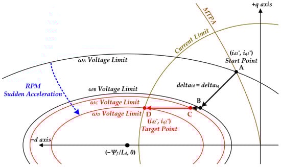
Figure 4.
Trajectory of the current reference vector in the d–q axis under a fixed ramp slope during rapid acceleration.
In the segment, both the d-axis and q-axis currents decrease at the same slope, resulting in a stable response within the voltage limit boundaries corresponding to ωA and ωB. In the segment, after the q-axis current reaches its target value iq2*, the d-axis current continues to decrease, placing the current vector at point C on the boundary of the voltage ellipse corresponding to ωC. In the segment, as the motor speed increases to ωD, the voltage ellipse shrinks, causing the current vector to move toward the final target point D (id2*, iq2*) while deviating outside the ellipse. Under this condition, the inverter operates in the overmodulation region, which may lead to voltage command saturation, output current distortion, and response delay.
This issue arises because a fixed ramp slope fails to account for the reduction in the voltage margin as the speed increases, and it becomes more pronounced during rapid acceleration when the q-axis command reaches its target before the d-axis command follows. This indicates the necessity for a modification in the control structure that allows the current command transition rate to be adjusted in real time according to the operating conditions. In transient conditions, the rate of change of the current appearing in the voltage equation can contribute to the increase in the inverter output voltage. However, since the inductance values are not large, this effect is relatively minor, and the structural tendency of the current vector trajectory to exceed the voltage limit is considered the dominant factor. Therefore, this paper proposes a real-time current command rate adjustment strategy based on the voltage margin ΔV, with the aim of achieving stable control even in transient response regions.
Figure 5 shows the waveform of the inverter output voltage measured during an experiment based on an actual driving profile. The blue line represents the measured inverter output voltage, while the black dashed line indicates the voltage limit determined by the DC-link voltage and the PWM modulation method. The waveform shows that the output voltage exceeds the voltage limit during the rapid acceleration phase. This occurred because the rate of change of the d-axis and q-axis current references was set identically, resulting in a temporary violation of the voltage limit during the transient period. Such an exceedance of the voltage limit is a critical issue that directly affects the controller’s performance. In general, in high-speed regions, the magnitude of the voltage demanded by the motor becomes significantly large, and the output voltage of the current controller may exceed the physical output limit of the inverter. In this case, the inverter can only produce its maximum achievable voltage, resulting in saturation of the controller’s voltage command. Once the voltage command is saturated, the PWM modulator enters a nonlinear operating region, where the switching duty is fixed at extreme values close to 0% or 100%, and the inverter output voltage can no longer linearly track the controller command. Consequently, the output of the current controller is distorted from the intended control signal, and the internal feedback path of the controller is also affected.
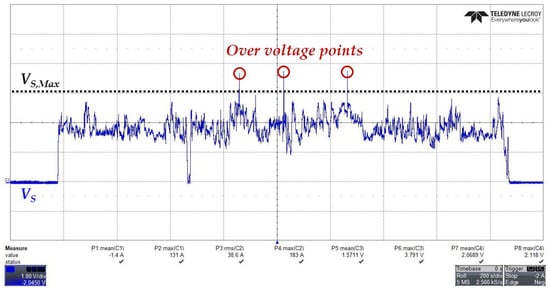
Figure 5.
Inverter output voltage waveform during a profile test under conventional control.
As a result, excessive overshoot, slow convergence, and abnormal distortion in the current response occur, leading to a degradation in torque control responsiveness and stability. This phenomenon is further aggravated under high-temperature driving conditions or heavy system loads, making it a critical factor for ensuring the reliability of EV drive systems. To prevent controller distortion caused by voltage saturation, the rate of change of the current command must be adjusted according to the operating conditions and the voltage margin. In particular, during transient intervals, such as rapid acceleration, the transition speed of the d-axis current responsible for field-weakening must be actively regulated to ensure that the inverter does not exceed the voltage limit. This is essential for preventing performance degradation due to saturation and for maintaining the overall stability of the system.
3. Proposed Control Strategy for Enhancing Transient-State Stability
In this section, the structure and operating principle of the proposed control strategy are described. Unlike conventional approaches that use a fixed and arbitrary value for the rate of change in the current reference, the proposed control strategy dynamically adjusts the ramp slope of the d-axis current reference in real time based on the voltage margin between the inverter output voltage and its maximum limit, thereby ensuring stable control within the voltage constraint region.
Figure 6 illustrates a current control block diagram incorporating the proposed control strategy. The overall controller structure is similar to the conventional one, consisting of a LUT-based current reference extractor, ramp generator, PI current controller, and PWM inverter. The key difference lies in the internal logic of the ramp generator, where the slope of the d-axis current reference is adaptively adjusted.
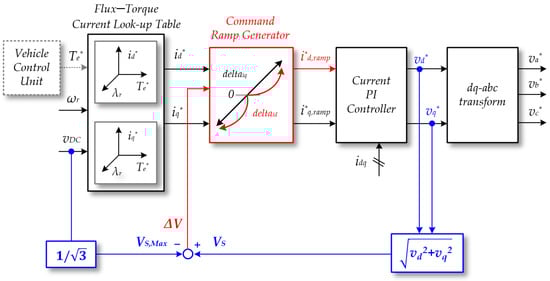
Figure 6.
Proposed IPMSM controller structure for xEV applications.
The control block diagram shown in Figure 6 calculates the magnitude of the output voltage vector VS, as expressed in (8), based on the d-axis and q-axis voltage commands vd* and vq* obtained from the current controller.
Meanwhile, the maximum output voltage VS,Max that the inverter can produce varies depending on the modulation method. In this study, based on space vector PWM (SVPWM), the maximum achievable output voltage is defined as (9). The voltage margin ΔV, obtained by comparing these two values, plays a key role in determining deltaid, the rate of change of the d-axis current command in the proposed control strategy.
The core concept of the proposed control method is to asymmetrically configure the ramp slopes of the d-axis and q-axis current references. In general, the q-axis current, which directly influences torque output, maintains a constant ramp slope to ensure torque responsiveness, whereas the d-axis current, which can directly reduce motor voltage through field-weakening, is adjusted with a variable rate of change depending on the operating condition. As a result, the method guides the system to remain within the voltage limit by controlling the transition path of the d-axis current vector.
Meanwhile, the control strategy proposed in this paper does not modify or replace the internal algorithm of the current controller; rather, it serves as a supplementary approach to mitigate transient phenomena that occur during the transfer of the current commands generated at a higher level to the controller. In particular, it aims to address abrupt command changes and entry into the overmodulation region, which arise when LUT-based current commands are updated relatively slowly due to the difference in communication cycles between the vehicle controller and the inverter. The proposed strategy is applicable regardless of the internal structure of the current controller and is intended to assist in maintaining the stable operation of an existing PI-based controller.
In the proposed control method, the rate of change of the d-axis current reference is determined by Equation (10), which is based on the voltage margin of the inverter and serves as a key strategy to prevent the voltage limit from being exceeded. In this equation, k is a scaling factor used to adjust the rate of change of the current reference according to the voltage margin, and deltaid,Max and deltaid,Min are determined experimentally by considering the control cycle and current response characteristics of the system.
The first condition in Equation (10) corresponds to the case where the d-axis current reference id*Curr obtained from the LUT in the current control cycle must change to a more negative value than the previous cycle’s reference id*Prev. This situation requires rapid and sufficient field-weakening to quickly and adequately secure the voltage margin against the voltage rise caused by an increase in the q-axis current or motor speed. When the voltage margin is small, the inverter output voltage is close to its voltage limit, and thus faster field-weakening is required; in this case, deltaid is set to a larger value close to deltaid,Max. Conversely, the second condition in Equation (10) represents the case where the magnitude of the negative d-axis current reference decreases, indicating a reduction in the field-weakening effect. When the magnitude of the d-axis current reference is decreasing and the voltage margin is small, an excessively rapid reduction can cause the voltage limit to be exceeded. Therefore, deltaid is set to a smaller value close to deltaid,Min, that is, a gentler slope, to ensure control stability. This strategy enables the d-axis current to proactively secure or maintain the voltage margin through field-weakening when the q-axis current either increases or decreases. By adjusting the rate of change of the d-axis current reference considering both the voltage margin and the direction of the reference change, control stability and torque responsiveness can be simultaneously achieved within the voltage-limit region.
The logic for calculating the change in the current command is implemented in two independent loops according to the controller execution structure. Figure 7 illustrates a flowchart of the implementation procedure for the proposed d-axis current command adjustment strategy. The overall control structure comprises the “LUT reference update loop,” which periodically updates the current commands extracted from the LUT in the upper-level controller, and the “inner control loop,” which operates at high speed in synchronization with the inverter’s internal controller. The LUT reference update loop operates at the communication cycle of the upper-level or vehicle controller (e.g., <1 kHz), extracts the d-axis current command id*Curr from the LUT, and updates the stored variable id*Prev for comparison with the previous value. The inner control loop operates at the current control cycle of the inverter (e.g., >8 kHz) and, in each control cycle, calculates the voltage margin between the present output voltage and the voltage limit. Based on this margin, either (10) or (11) is applied to compute the corresponding change deltaid, which is accumulated in the ramped current command id*ramp at every control cycle and is ultimately delivered to the current controller. By considering the difference between the two update cycles, the proposed algorithm evaluates the voltage margin and the direction of the command change in each control cycle with reference to the upper-level LUT command, determines the appropriate deltaid, and applies it cumulatively to achieve smooth and stable tracking of the current command.
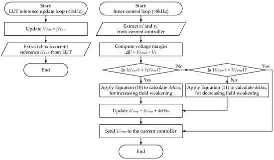
Figure 7.
Flowchart of the proposed d-axis current reference ramp control strategy with a dual-loop structure.
In practical xEV applications, the characteristics of an IPMSM vary depending on factors such as the internal structure, winding configuration, and cooling method. In particular, the inductance and flux exhibit nonlinear behavior, changing in real time according to the current magnitude and operating conditions. Accurately tracking these parameters and reflecting them in the control imposes a significant computational burden and increases implementation complexity. Therefore, this study aims to develop a control strategy that is insensitive to such parameter variations, applicable to various IPMSM structures, and suitable for real-time implementation. To this end, instead of employing a complex parameter-based modeling approach, an indirect control method is proposed that utilizes the voltage margin ΔV. The value of ΔV is determined from the output voltage calculated in the inverter controller, the DC-link voltage (e.g., battery voltage), and the maximum achievable output voltage VS,Max determined by the PWM method. This quantity can be computed in real time and serves as an effective indicator that concisely reflects the physical constraints of the system. In the proposed control strategy, the d-axis current command change is adjusted according to the magnitude of ΔV, thereby preventing voltage limit exceedance during transient intervals and achieving a more stable control response.
Figure 8 compares the simulation results of the conventional fixed-slope method and the proposed d-axis current slope adjustment strategy under conditions simulating the rapid acceleration of an HEV-specification IPMSM. Figure 8a shows the results of the conventional method, while Figure 8b presents the results of the proposed method. The red line represents the real-time voltage vector trajectory of the inverter, and the blue line indicates the voltage limit boundary defined by the PWM modulation method. With the conventional method, abrupt changes in the current commands during the transient interval caused the output voltage to exceed the voltage limit, resulting in a peak-to-peak voltage ripple of up to 29.9 V in the inverter output voltage, which can lead to degraded control stability. In contrast, the proposed method maintains the same starting and target points but adjusts the slope of the d-axis current command according to the real-time voltage margin ΔV, ensuring that the voltage vector remains within the voltage limit boundary throughout the process. As a result, the voltage ripple during the transient interval was stably suppressed to a maximum of 4.4 V. These results demonstrate that the proposed method effectively prevents voltage saturation and ensures the stability of current control by dynamically adjusting the change in the d-axis current command based on the real-time voltage margin ΔV. The method achieves stable control performance with simple computations, which makes it highly practical. Table 1 summarizes the key parameters of the motor used in the simulation, while Table 2 presents a quantitative comparison of the performance metrics for each control method. In particular, the total harmonic distortion (THD) of the phase current was reduced from 4.32% with the conventional method to 3.52% with the proposed method, and the peak phase current and peak DC input current were each reduced by approximately 8%. The peak output voltage and voltage ripple were also significantly reduced, indicating that the proposed control strategy can improve both control stability and energy efficiency during transient intervals.
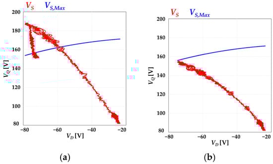
Figure 8.
Simulation results comparing control methods: (a) conventional fixed ramp control and (b) proposed adaptive ramp control.

Table 1.
Motor parameters used in the simulation model.
Table 2.
Comparison of simulation results between the conventional and proposed methods.
4. Experimental Verification
To validate the effectiveness of the proposed control strategy, a dynamometer test environment was constructed using a 38 kW class IPMSM and an inverter designed for HEV specifications. Figure 9 presents the dynamometer test configuration along with the IPMSM used in the experiment. To replicate a range of real-world driving conditions in the experiment, four different speed–torque profiles were applied in the experiment, and the performance difference between the conventional control method and the proposed strategy was analyzed accordingly. The detailed specifications of the motor used in the experiment are listed in Table 3, and the experiment aimed to quantitatively verify the effectiveness of the proposed control strategy, particularly in terms of stability during transient conditions. The IPMSM used in the experiments was a commercial HEV motor, and the model employed in the simulations was configured based on the parameters of this experimental motor. Therefore, both the experiments and simulations were conducted using the same electrical parameters (R, Ld, Lq, p, ψf), enabling direct comparison and validation between the experimental and simulation results.
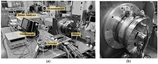
Figure 9.
Experimental setup: (a) dynamometer test bench and (b) IPMSM used in the HEV application.
Table 3.
Specifications of the IPMSM used in the experimental setup.
In this study, the performance of the proposed control strategy was verified under conditions representative of actual driving by constructing driving profiles based on real vehicle data from a hybrid vehicle. The driving data were acquired using an in-vehicle CAN communication-based data logging system. Four speed–torque profiles were defined, as shown in Figure 10a,b correspond to urban driving modes 1 and 2, while (c) and (d) correspond to highway driving modes 1 and 2. Each profile contained approximately 30 min of data and was designed to represent realistic and frequently occurring driving conditions, emphasizing driving patterns with frequent variations in speed and torque to evaluate the transient response characteristics of the controller. The red lines indicate the torque commands of each profile, while the blue lines represent the speed commands. These profiles adequately reflect rapid acceleration and deceleration conditions that can occur in real vehicle operation.
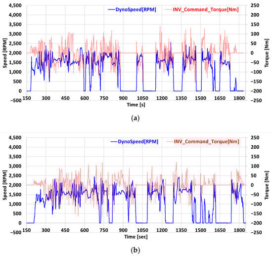
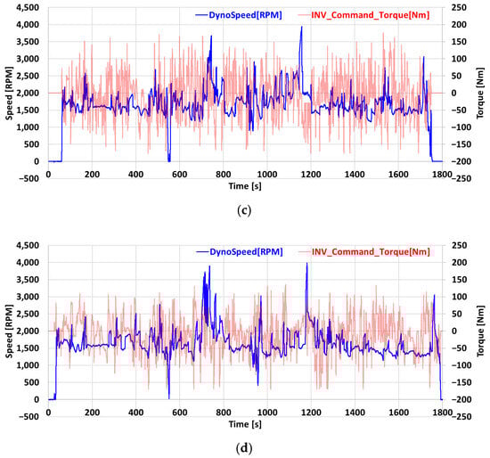
Figure 10.
Torque–speed profiles simulating HEV operation: (a) urban driving mode 1, (b) urban driving mode 2, (c) highway driving mode 1, and (d) highway driving mode 2.
To clearly and quantitatively analyze the cumulative performance differences in the proposed control strategy under real driving conditions, the average torque error and DC energy consumption were compared between the conventional method and the proposed method using four speed–torque profiles. The comparison results are summarized in Table 4 and Table 5, where Table 4 presents the average torque error for each driving mode, and Table 5 presents the DC energy consumption over the entire driving period. For each metric, the improvement in the proposed method over the conventional method is also expressed as a percentage to explicitly indicate the quantitative level of performance enhancement. The average torque error is defined as the mean value obtained by integrating the absolute instantaneous error between the reference torque and the actual output torque over the entire driving profile and dividing it by the total time. This metric was included to quantitatively evaluate how accurately and stably the controller output tracks the target torque, enabling an objective comparison of not only the torque response characteristics but also the tracking performance during both transient and steady-state intervals. The DC energy consumption is calculated as the accumulated value obtained by integrating the DC power at the inverter input over time during the profile test, representing the net amount of electrical energy consumed or recovered for vehicle propulsion over the entire driving cycle. This metric was included to evaluate the impact of control strategy differences on inverter input power consumption and to comprehensively compare the power usage efficiency and net energy consumption characteristics throughout the driving cycle. The reason the DC energy consumption shown in Table 5 appears as a negative value is that the driving profiles used in this study were configured based on an HEV environment without an external battery charging function and under conditions designed to prevent a decrease in the battery state of charge (SOC). Specifically, the overall driving profiles were designed such that the energy recovered through regenerative braking exceeds the energy used for propulsion, resulting in a cumulative negative DC energy consumption.
Table 4.
Comparison of the conventional and proposed methods in terms of torque error under four different speed–torque driving profiles.
Table 5.
Comparison of the conventional and proposed methods in terms of DC energy consumption under four different speed–torque driving profiles.
The analysis results indicate that, in the urban driving modes, there was no significant performance difference between the conventional and proposed methods. This is because, under low-speed operating conditions, the inverter output voltage is unlikely to reach the voltage limit, thereby reducing the influence of transient responses. In contrast, in the highway driving modes, a distinct performance difference was observed. High-speed driving contains frequent transient events, and under these conditions, the proposed method achieved greater improvements in both torque response error and DC energy consumption. These results demonstrate that, when the motor operates beyond the base speed in the high-speed region, the inverter output voltage approaches the voltage limit. If the current commands change abruptly in this situation, the controller may fail to respond stably, resulting in torque instability and unnecessary current consumption. This issue is more pronounced in EV drive systems in which LUT-based current commands are updated discontinuously in each communication cycle. The proposed control strategy addresses these issues by adjusting the change in the d-axis current command in real time according to the magnitude of ΔV, thereby suppressing voltage exceedance and current distortion during transient states. The experimental results verify that this approach enhances both the control stability and the energy efficiency of the overall system.
Figure 11 compares the inverter output voltage waveforms in the high-speed and urban driving modes before and after applying the proposed method, serving as comparative data to supplement the quantitative analysis results presented in Table 4 and Table 5. The figure is designed to visually examine the output voltage response characteristics during transient intervals and to compare, at the waveform level, how the intervals of modulation limit exceedance change when the proposed method is applied compared to the conventional method. In the high-speed driving mode, frequent exceedance of the modulation limit voltage occurs due to rapid changes in speed and torque, primarily in the field-weakening region. Under such transient conditions, distortion of the phase currents and inverter input current can occur, leading to reduced control stability. The proposed d-axis current reference rate adjustment strategy contributes to mitigating transient responses by suppressing such modulation limit exceedance, as demonstrated in the waveforms in Figure 11. For a more intuitive comparison, the modulation limit voltage is indicated with a black dashed line, and instances of exceedance are highlighted with red circles. In contrast, in the urban driving mode, voltage limit exceedance is rarely observed, and the differences between the two methods are relatively small.
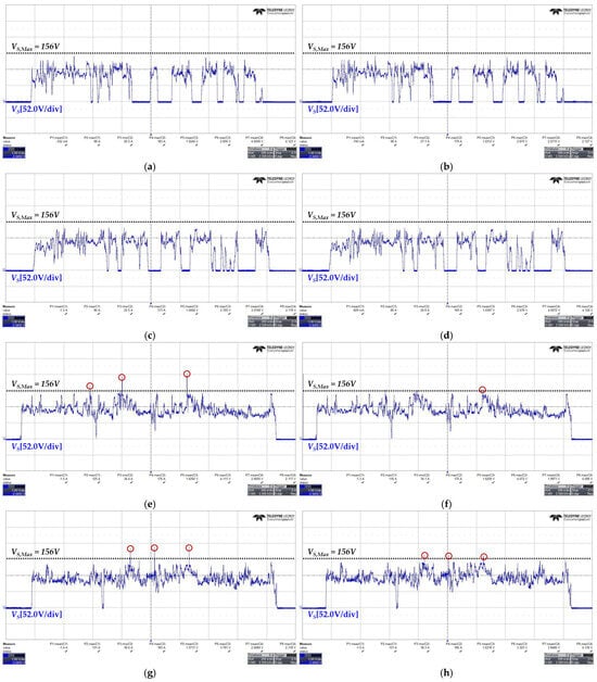
Figure 11.
Inverter output voltage waveforms under four different driving profiles before and after applying the proposed method. Over-limit points exceeding the modulation boundary are highlighted. (a,b) Urban driving mode 1: before and after applying the proposed method; (c,d) urban driving mode 2: before and after; (e,f) highway driving mode 1: before and after; (g,h) highway driving mode 2: before and after.
As noted earlier, the red circles in Figure 11 indicate transient intervals in the high-speed driving modes where the output voltage approached or exceeded the modulation limit. The operating conditions of these six events—including speed change, torque change, and transient duration—are summarized in Table 6, while the performance indicators for each event—maximum THD, peak phase current, peak DC input current, peak output voltage, and the maximum VS/VS,Max—are presented in Table 7. These results quantitatively confirm that the proposed method reduced both the magnitude and duration of modulation limit exceedance in all events, and in most cases, lowered current and THD, thereby demonstrating its effectiveness in mitigating transient responses.
Table 6.
Operating conditions for the six voltage-limit proximity or over-limit transient events (red circles in Figure 11), including speed change, torque change, and transient duration for each case.
Table 7.
Performance indicators for the six events in Table 6, comparing the conventional (Conv.) and proposed (Prop.) control strategies in terms of maximum THD, peak phase current, peak DC input current, peak output voltage, and the maximum value of VS/VS,Max.
To analyze the transient response characteristics of the proposed control strategy in greater detail, additional sensitivity tests were performed for the parameter k, which serves as the response gain to the voltage margin ΔV. The results are presented in Figure 12. This test simulated a transient scenario within the highway driving profile in which the motor accelerated from 1090 RPM to 3820 RPM while simultaneously transitioning from regenerative braking (−55 Nm) to motoring mode (+105 Nm). This transition occurred over approximately 0.9 s, and the current response characteristics for different k values were compared to assess the response characteristics and stability of the proposed control method. To quantitatively evaluate the performance of the proposed control strategy during the transient interval in Figure 12, additional performance metrics were extracted and summarized in Table 8. The quantitative results in Table 8 are based on data measured at the point within the transient response where the system stability was most degraded. In particular, the THD of the phase currents was calculated around the time instant when waveform distortion was most severe. As shown in Figure 12, smaller k values reduce the sensitivity to the voltage margin ΔV, thereby decreasing the change in the d-axis current command. As a result, sufficient field-weakening is not achieved during acceleration, leading to extended intervals in which the voltage limit ellipse is exceeded. Consequently, as observed in Table 8, distortion appears in both the phase current and inverter input current waveforms, and control stability degrades during the transient interval. In contrast, when k is set to an appropriate value, a balance between the response speed and stability of the current command is achieved, resulting in rapid convergence of the transient response and a reduction in current overshoot.
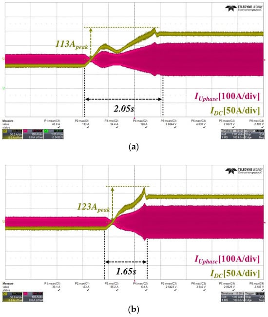
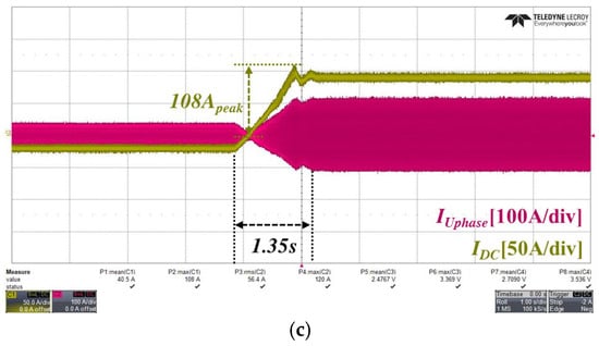
Figure 12.
Comparison of current responses for different values of the coefficient k during a simulated transient event in a highway driving profile (acceleration from 1090 RPM to 3820 RPM and torque transition from −55 Nm to + 105 Nm over approximately 0.9 s). (a) k = 0.00015; (b) k = 0.00020; (c) k = 0.00025.
Table 8.
Quantitative comparison of transient performance according to the coefficient k (based on Figure 12).
Additionally, although the proposed control strategy was developed and validated for an IPMSM used in electric vehicle traction applications, the underlying principle can also be applied to other types of synchronous machines such as SPMSMs, WRSMs, SynRMs, and PMa-SynRMs. SPMSMs have no rotor saliency, resulting in a very limited field-weakening range, and the improvement in high-speed performance is generally smaller compared to IPMSMs. WRSMs can directly control the air-gap flux through the rotor winding, offering potentially greater benefits at high speeds, but the brush and slip-ring structure limits their use as main traction motors. SynRMs operate without permanent magnets and produce torque solely through rotor saliency, allowing field-weakening operation but with lower torque density, making them less suitable for vehicle traction. PMa-SynRMs incorporate small permanent magnets into a SynRM rotor to improve torque density and efficiency, enabling a certain degree of field-weakening capability and potential performance benefits from the proposed strategy, though still to a lesser extent than in IPMSMs.
5. Conclusions
This study proposes a current reference generation strategy to enhance the transient response stability of an IPMSM controller in xEV drive systems. In conventional controller structures, the d-axis and q-axis current references are updated at the same rate, determined by a fixed ramp slope. This approach can lead to situations where the inverter output voltage exceeds its voltage limit, particularly during transients such as rapid acceleration or deceleration at high speeds. To address this issue, the proposed strategy controls the d-axis current reference by dynamically adjusting its rate of change in real time based on the voltage margin, defined as the difference between the inverter output voltage and its limit. This ensures that the voltage vector remains within the allowable range. The proposed method prevents voltage overshoot and simultaneously preserves the responsiveness of the q-axis current. As a result, both overall control stability and torque response performance are ensured. The effectiveness of the proposed control strategy was verified through dynamometer testing with an IPMSM configured for HEV specifications. The experimental results based on various speed–torque profiles that emulate real driving conditions showed minimal difference between the proposed and conventional methods under urban driving modes. However, under highway driving modes, significant improvements were observed in terms of torque response error and energy consumption. In addition, the inverter output voltage waveforms confirmed that the proposed method stably controls the system during transient periods, preventing significant violation of the voltage limit. In conclusion, the current reference rate adjustment strategy proposed in this study is an effective control approach that satisfies both transient performance and voltage constraint requirements. It is expected to contribute to improved stability and efficiency of IPMSM drive systems under high-speed and high-load conditions in future applications.
Author Contributions
Conceptualization, Y.S., S.C. and J.L.; methodology, Y.S. and S.C.; software, Y.S.; validation, Y.S. and S.C.; formal analysis, Y.S., S.C. and J.L.; investigation, Y.S. and S.C.; data curation, Y.S.; writing—original draft preparation, Y.S.; writing—review and editing, S.C. and J.L.; supervision, S.C. and J.L.; project administration, S.C. and J.L. All authors have read and agreed to the published version of the manuscript.
Funding
This research was supported by the Automotive Industry Technology Development Program (2410012302, Development of High Power Density Electric Traction System for EV with Multi pole(over 12poles) Traction Motor) funded by the Ministry of Trade, Industry and Energy (MOTIE, Korea).
Data Availability Statement
The original contributions presented in this study are included in this article. Further inquiries can be directed to the corresponding author.
Conflicts of Interest
The authors declare no conflicts of interest.
References
- Liu, X.; Chen, H.; Zhao, J.; Belahcen, A. Research on the Performances and Parameters of Interior PMSM Used for Electric Vehicles. IEEE Trans. Ind. Electron. 2016, 63, 3533–3545. [Google Scholar] [CrossRef]
- Wu, J.; Wang, J.; Gan, C.; Sun, Q.; Kong, W. Efficiency Optimization of PMSM Drives Using Field-Circuit Coupled FEM for EV/HEV Applications. IEEE Access 2018, 6, 15192–15201. [Google Scholar] [CrossRef]
- Dang, L.; Bernard, N.; Bracikowski, N.; Berthiau, G. Design Optimization with Flux Weakening of High-Speed PMSM for Electrical Vehicle Considering the Driving Cycle. IEEE Trans. Ind. Electron. 2017, 64, 9834–9843. [Google Scholar] [CrossRef]
- Yu, L.; Zhang, Y.; Huang, W. Accurate and Efficient Torque Control of an Interior Permanent Magnet Synchronous Motor in Electric Vehicles Based on Hall-Effect Sensors. Energies 2017, 10, 410. [Google Scholar] [CrossRef]
- Harnefors, L.; Pietilainen, K.; Gertmar, L. Torque-maximizing field–weakening control: Design, analysis, and parameter selection. IEEE Trans. Ind. Electron. 2001, 48, 161–168. [Google Scholar] [CrossRef]
- Lin, F.-J.; Liao, Y.-H.; Lin, J.-R.; Lin, W.-T. Interior Permanent Magnet Synchronous Motor Drive System with Machine Learning-Based Maximum Torque per Ampere and Flux-Weakening Control. Energies 2021, 14, 346. [Google Scholar] [CrossRef]
- Stumpf, P.; Tóth-Katona, T. Recent Achievements in the Control of Interior Permanent-Magnet Synchronous Machine Drives: A Comprehensive Overview of the State of the Art. Energies 2023, 16, 5103. [Google Scholar] [CrossRef]
- Nandi, A.K.; Chakraborty, D.; Vaz, W. Design of a comfortable optimal driving strategy for electric vehicles using multi-objective optimization. J. Power Sources 2015, 283, 1–18. [Google Scholar] [CrossRef]
- Krasopoulos, C.T.; Beniakar, M.E.; Kladas, A.G. Velocity and torque limit profile optimization of electric vehicle including limited overload. IEEE Trans. Ind. Appl. 2017, 53, 3907–3916. [Google Scholar] [CrossRef]
- Xu, G.; Xu, K.; Zheng, C.; Zhang, X.; Zahid, T. Fully Electrified Regenerative Braking Control for Deep Energy Recovery and Maintaining Safety of Electric Vehicles. IEEE Trans. Veh. Technol. 2016, 65, 1186–1198. [Google Scholar] [CrossRef]
- Jung, S.; Hong, J.; Nam, K. Current Minimizing Torque Control of the IPMSM Using Ferrari’s Method. IEEE Trans. Power Electron. 2013, 28, 5603–5617. [Google Scholar] [CrossRef]
- Prabhu, N.; Thirumalaivasan, R.; Ashok, B. Critical Review on Torque Ripple Sources and Mitigation Control Strategies of BLDC Motors in Electric Vehicle Applications. IEEE Access 2023, 11, 115699–115739. [Google Scholar] [CrossRef]
- Bianco, E.; Rubino, S.; Carello, M.; Bojoi, I.R. Advanced Torque Control of Interior Permanent Magnet Motors for Electrical Hypercars. World Electr. Veh. J. 2024, 15, 46. [Google Scholar] [CrossRef]
- Tripathi, A.; Khambadkone, A.M.; Panda, S.K. Dynamic Control of Torque in Overmodulation and in the Field Weakening Region. IEEE Trans. Power Electron. 2006, 21, 1091–1098. [Google Scholar] [CrossRef]
- Lerdudomsak, S.; Doki, S.; Okuma, S. Analysis for Unstable Problem of PMSM Current Control System in Overmodulation Range. In Proceedings of the IEEE Industry Applications Society Annual Meeting, Edmonton, AB, Canada, 5–9 October 2008; pp. 1–8. [Google Scholar]
- Zhou, C.; Yang, G.; Su, J. PWM Strategy with Minimum Harmonic Distortion for Dual Three-Phase Permanent-Magnet Synchronous Motor Drives Operating in the Overmodulation Region. IEEE Trans. Power Electron. 2016, 31, 1367–1380. [Google Scholar] [CrossRef]
- Shin, Y.; Cho, S.; Lee, D.; Seol, H.; Ryu, J.; Koo, G. Control Strategy to Improve Control Stability in Transient states of PMSM for xEV. In Proceedings of the IEEE Transportation Electrification Conference and Expo (ITEC), Chicago, IL, USA, 19–21 June 2024; pp. 1–6. [Google Scholar]
Disclaimer/Publisher’s Note: The statements, opinions and data contained in all publications are solely those of the individual author(s) and contributor(s) and not of MDPI and/or the editor(s). MDPI and/or the editor(s) disclaim responsibility for any injury to people or property resulting from any ideas, methods, instructions or products referred to in the content. |
© 2025 by the authors. Licensee MDPI, Basel, Switzerland. This article is an open access article distributed under the terms and conditions of the Creative Commons Attribution (CC BY) license (https://creativecommons.org/licenses/by/4.0/).