Abstract
Microgrids play a crucial role in the development of future smart grids, with multiple interconnected microgrids forming large-scale multi-microgrid systems that operate as smart grids. Multi-agent system (MAS)-based control solutions are the most suitable for addressing such control challenges. This paper presents a demand-side management (DSM) strategy using a meta-heuristic optimization technique for minimizing the household energy consumption cost using MAS. The binary grey wolf optimization algorithm (BGWOA) optimizes load scheduling, reducing electricity costs, without compromising consumer preferences using time-of-day (ToD) tariffs. The communication agents and load agents comprise the MAS used to streamline load control operations. The results demonstrate that MAS-based load control using metaheuristic optimization techniques enhances demand-side management, thus minimizing the electricity costs while adhering to contradictory parameters like user preferences, appliance duration, and load atomicity. This makes renewable energy integration more cost-effective in smart grids, thereby ensuring affordable, reliable, and sustainable energy for all.
1. Introduction
Smart grids and microgrids are key enablers of the UN Sustainable Development Goals (SDGs), especially SDG 7 (affordable and clean energy) and SDG 11 (sustainable cities). Smart grids enhance energy efficiency, integrate renewables, and improve real-time energy management, making urban systems more resilient and sustainable [1]. Microgrids support rural electrification by leveraging local renewable resources, offering scalable and decentralized energy solutions [2]. When multiple microgrids are interconnected, they form multi-microgrid (MMG) systems or microgrid clusters. These MMG systems, or microgrid clusters, boost energy reliability and adaptability, contributing to a decentralized smart energy network that supports sustainable development in both urban and rural areas [3].
Smart grids can be envisioned as networks of interconnected microgrids, thus redefining modern power systems by enabling a reliable and uninterrupted energy supply through the seamless integration of renewable energy sources [4]. This decentralized and intelligent architecture enhances grid flexibility and resilience, addressing challenges arising from the exponential growth in electricity demand and the inherent limitations of conventional power systems [5,6]. The evolving power demands of the 21st century are being effectively addressed through smart grid architectures that facilitate real-time energy management, bidirectional power flow, and seamless integration of rooftop solar and other distributed energy resources [7].
The technological advancement for the integration of renewable energy resources like photovoltaic (PV) solar energy and battery energy storage systems (BESS) has transformed each household into a smart microgrid [8], thus transforming the role of consumers into prosumers [9,10]. This transformation in the role of consumers opens new research perspectives for demand-side management in power systems [11]. Early research has given limited consideration to consumer behavior patterns and economic factors in the power consumption of households. Optimal load scheduling is foundational to intelligent, sustainable, and user-centric energy systems. It benefits individual households and contributes to enhancing grid efficiency, reliability, and the transition to clean energy [12]. The opportunities that renewable energy resources (RERs) and BESS have provides several dimensions for research in demand-side management [13]. Demand-response (DR) programs have been successfully implemented to achieve economic benefits with lower carbon emissions and streamlined usage patterns of prosumers [14,15].
Demand-side management, through load scheduling, can be formulated as a mixed-integer linear programming (MILP) optimization problem [16]. MILP is an optimization method used to formulate and solve cost minimization problems, capable of obtaining the global optimum when solved to optimality [17]. Residential electrical loads are classified into three main categories: critical loads, which require immediate, fixed-time operation (e.g., lights and fans); atomic controllable loads, which must run uninterrupted once started (e.g., washing machines); and nonatomic controllable loads, which can be interrupted and rescheduled within a time window (e.g., heating, ventilation, and air conditioning (HVAC) systems and electric vehicle (EV) chargers). This classification helps in managing energy usage more efficiently [18]. However, the MILP approach has certain limitations in representing multiple objectives and ensuring uninterrupted scheduling of household atomic loads.
From the literature [18,19], it is evident that metaheuristic approaches provide greater flexibility in problem representation, making them more suitable for controlling atomic household loads. According to [20], the grey wolf optimizer (GWO) outperforms particle swarm optimization (PSO) and genetic algorithms (GAs) in terms of convergence speed and the ability to avoid local minima through more effective exploration. As reported in [21], it outperforms PSO in solving discrete optimization challenges and mixed-integer linear programming tasks, including load scheduling, economic dispatch, and unit commitment. Furthermore, although genetic algorithms (GAs) can manage a large number of variables in optimization problems, GWO has been shown to perform more effectively in high-dimensional search spaces, as highlighted in [22,23]. Therefore, BGWOA was adopted in this study due to its ease of implementation, scalability, stability, and effectiveness in solving discrete and mixed-integer optimization problems.
In DR programs, time-of-use (ToU) pricing serves as a key mechanism for optimizing residential electricity consumption by incentivizing consumers to shift usage away from peak periods. A comparative study by Khan et al. [24] analyzed various dynamic pricing strategies, including ToU, critical peak pricing (CPP), and real-time pricing (RTP). While RTP offers greater potential for responsiveness and cost savings under dynamic conditions, ToD pricing is often more effective in environments with relatively stable consumption patterns due to its simplicity and predictability. ToD pricing is a specified implementation of ToU pricing, where electricity rates vary based on fixed daily time blocks, unlike ToU, which may incorporate seasonal or day-type variations. Accordingly, this paper adopted the ToD pricing model for load optimization.
MAS has been extensively used in large-scale and complex applications [17,25,26]. However, research on MAS-based demand-side management using metaheuristic optimization remains limited. In this study, MAS was adapted for load control by employing load agents only, reducing the complexities associated with managing multiple agents. This streamlined approach enhances efficiency and ensures effective load control.
Although numerous DSM studies have focused on optimization, only a limited number have incorporated the proposed solutions within a simulation environment for validation. Discrete variants of metaheuristic optimization algorithms, such as BGWOA, are well-suited for binary load-level scheduling but are largely absent from existing studies. Despite its potential benefits, the development of a unified cost-based multi-objective function that integrates energy cost, load priority, delay cost, and incentive values—expressed in a common unit (INR)—has received little attention in DSM research. Addressing the above-mentioned research gaps, the main contributions of this paper are as follows:
- A unified cost-based multi-objective function is formulated to combine energy cost, load priority, delay cost, and incentive values—each expressed in the same unit (INR). This approach eliminates the need for normalization or arbitrary weighting, thereby simplifying interpretation and enhancing mathematical clarity. Furthermore, using real monetary values for priority and delay penalties directly reflects user-centric preferences in cost terms. The optimization is implemented using BGWOA.
- Using scenario-based validation with distributed energy resource (DER) integration, the system is tested across three practical scenarios, including configurations with and without solar PV and BESS. The microgrid model is implemented using Simulink (MATLAB R2021b), and MAS implementation is developed using Simulink Stateflow to create the validation environment.
2. Problem Formulation
The objective of the DSM problem is to find an optimal schedule of operation so that the electricity bill of the consumer is minimized with the given tariff structure and the load parameters. Shiftable loads are shifted without violating the maximum demand limit imposed by the utility to minimize the electricity cost. DR programs use different tariff structures like ToU, CPP, and RTP. In this study, the ToD tariff provided by KSEB (Kerala State Electricity Board), Kerala, India [27], was used.
2.1. Load Modeling
Household load scheduling, which optimizes appliance operation based on electricity pricing, is a key component of residential DSM. It aims to minimize both peak-hour energy consumption and total electricity cost while ensuring user comfort and adherence to operational constraints.
This study considered the load scheduling problem as an optimization-based DSM strategy that balances user comfort, appliance constraints, and cost minimization under a ToD pricing scheme. Here, focus was given to critical and controllable loads, both atomic in nature.
The problem was mathematically formulated for 24 h. T indicates the 24 hourly time intervals within a day.
Each load was modeled using eight parameters. As shown in Table 1, each load is characterized by
| starting time slot at which the execution of the load starts. | |
| finishing time slot at which the execution of the load ends. | |
| baseline starting time, prefered time slot at which the execution of the load starts. | |
| baseline finishing time, prefered time slot at which the execution of the load ends. | |
| total number of time slots used by the load to complete its execution. | |
| power rating of the load in kW. | |
| priority factor used to prioritize the execution of the load. Unit in rupees. | |
| delay coefficient associated with the load that is used to represent the inconvenience associated with shifting the operation of said load. Unit in rupees. |

Table 1.
Load parameters.
The start time ( = 6) and finish time ( = 9) define the flexible operating window for . Within this interval, the load requires ( = 2) time slots to complete its execution. The user-preferred or baseline schedule specifies a start time of ( = 6) and a finish time of ( = 7), reflecting the ideal time slot as defined by the user. The rated power of is ( = 3 kW).
Load prioritization is determined using a priority factor (), where a lower value indicates higher priority. For instance, loads with ( = 1) are scheduled before those with ( = 2), ensuring that higher-priority tasks are executed earlier in the schedule. The delay penalty () quantifies the user’s inconvenience cost associated with shifting the load from its baseline schedule. For , a delay penalty of ( = 5) represents the penalty incurred per time slot of delay. For higher-priority loads, a larger delay penalty (e.g., = 10) is assigned to discourage extended postponement of their operation. In the case of , the maximum permissible delay is two time slots.
Delay penalty is a metric used to quantify the inconvenience experienced by consumers due to the postponement of controllable load operations [28]. The value of the delay penalty is selected based on the priority level of the load. For critical or high-priority appliances, the delay penalty is set higher than the average tariff (e.g., 10, given an average tariff of 7), thereby discouraging any significant scheduling deviation. In contrast, for controllable or low-priority loads, the delay penalty is assigned a value between 0 and the average tariff (e.g., 5), reflecting a higher tolerance to schedule shifts.
2.2. Optimization Problem
The demand-side management problem invovles minimizing the energy consumption cost from the utility grid.
2.2.1. Objective Function
The optimized load scheduling framework effectively balances the conflicting objectives of load prioritization and delay minimization. It enables the optimal scheduling of controllable household appliances under a time-of-day (ToD) pricing scheme, with the primary goal of minimizing electricity costs. This is achieved while satisfying key operational constraints, including user preferences, appliance runtime requirements, the inconvenience associated with load shifting, peak tariff avoidance, and the atomicity of load execution.
where
| is the time slot, . | |
| is the load, . | |
| is the total number of loads, which is 6. | |
| is the power source (utility grid and solar PV/BESS). | |
| is the total electricity cost. | |
| is the cost of electricity for the time slot t from source. | |
| is the rated power of in kW. | |
| is the variable indicating the ON/OFF status of at time slot t. |
The objective function formulated to minimize energy costs under the time-of-day (ToD) tariff structure is presented in Equation (3).
To incorporate load prioritization into the scheduling model, Equation (4) was developed by adding an additional term to Equation (3). This term, measured in rupees, is calculated as the product of the load’s priority factor, rated power, and binary load status. It guides the optimization process to favor schedules that align with the assigned priority levels of the loads, with higher-priority (lower-factor) loads scheduled earlier.
where
| is the priority factor of . Load priority is quantified in terms of rupees to reflect its relative importance in cost-based scheduling. |
The addition of the third term in Equation (5) to the existing objective function ensures optimal delay handling, particularly for lower-priority loads, by minimizing scheduling inconvenience within acceptable limits.
where
| denotes the delay penalty for , measured in monetary units (rupees). | |
| is the total delay (the number of time slots) that the was shifted during | |
| optimal scheduling. |
is calculated as follows:
where
| is the total number of time slots used by the to complete its execution. |
Here, in Equation (6), indicates the customer’s preferred pattern (expected operation time slots) of loads or devices. It is called the baseline operation schedule of appliances. The delay is calculated by finding the Euclidean distance between the baseline schedule and the optimal schedule generated [29].
A comparative study was conducted in [29] using different cases of load shifting and Equations (6) and (7). The results showed that the delay calculation was based on the Euclidean distance and was more appropriate than using absolute subtraction. Hence, in this paper, we used Equation (6) to calculate the delay.
The absolute subtraction method uses Equation (7) for delay calculation between the baseline schedule and the optimal schedule generated [30].
To promote beneficial behavior patterns in customers, incentives can be given to customers for shifting the load from peak period to off-peak period [30]. This is considered a smart method to indirectly control the load to cope with inadequate power generation. The customer’s behavioral pattern influences the baseline load pattern, leading to minimal energy costs.
Hence, Equation (5) can be rewritten by including a term connected to incentive, which is subtracted from the total cost calculation.
where represents the incentive value associated with each time slot t in the grid tariff structure. A fixed incentive of Rs 2 is offered during peak time slots to encourage load shifting, as referenced in [30]. This incentive acts as a negative cost in the objective function, effectively reducing the total energy expenditure for consumers who defer usage to high-tariff periods.
Thus, the multi-objective, constrained optimization problem with integer decision parameters can be formulated into a single-objective, constrained optimization problem using the linear weighted sum method and is mathematically formulated as follows:
Here, in Equation (9), , , , and represent the input parameters associated with the respective components of the multi-objective function, reflecting the relative importance of each objective [29,31,32]. Since all of the multiple objectives are measured in the same unit, depend on the same variable, and are interrelated, there is no need to normalize or assign weights for mathematical correctness. These objectives can be directly aggregated into a single composite objective function, preserving both the interpretability and correctness of the optimization model.
2.2.2. Constraints
The constraints are as given in Equations (10)–(13).
where
the load is in the “ON” state at its alloted time interval for slots only. This is similar to the case with .
where
is the maximum power demand limit set by the utility.
Equation (13) limits the power consumed at any time slot t, ensuring it is less than the permissible value set by the utility in kW. The value considered in this study was 20 kW.
3. Modeling of the Proposed System
3.1. MAS of the Proposed System
An MAS is a self-organizing computational framework composed of multiple intelligent agents that interact and cooperate to achieve a common objective. The suitability of MAS for solving complex engineering problems stems from key agent characteristics: autonomy, enabling independent decision-making; social ability, allowing communication through agent communication languages; reactivity, through environment-driven perception and response; and proactiveness, enabling timely and rational actions [33].
MAS break down a complex problem handled by a single entity like a centralized system into small simpler problems, which are handled by multiple entities similar to in a distributed system. MAS offer an efficient and flexible approach for scaling complex problems or systems, enabling distributed coordination and management as the system size or complexity increases [26].
System Architecture of the Proposed MAS System
The system architecture of the MAS system is shown in Figure 1. The BGWOA block and communication agent were implemented using MATLAB (2021b) script, while all other components were modeled in Simulink. The load agents were implemented using Simulink Stateflow, enabling efficient representation of their decision-making and control mechanisms. The microgrid contained a renewable energy source (Solar PV), connected to the microgrid using a boost converter. The battery system was incorporated into a microgrid to store excess solar energy generated. A voltage source inverter with an LCL filter was used to convert the DC power generated to AC. The microgrid was connected to the utility grid. Six loads were connected to the microgrid. The operational control of all six loads was carried out using load agents.
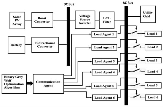
Figure 1.
System architecture of MAS the system.
The BGWOA block generated an optimal scheduling pattern (6 × 24 matrix) satisfying the objective function discussed earlier. The communication agent associated with the BGWOA block separated the operation pattern of each load (1 × 24 matrix) from the common load schedule. The operational pattern generated for each load was passed to corresponding load agents. Thes load agents controlled the “on” and “off” states of the loads using switches. The loads could be powered either by utility power or solar PV (if sufficient power was generated using solar PV). The MAS used for load control comprised communication and load agents. The load agent ensured that the load connected strictly following the operation pattern given by the optimization algorithm.
The operation of the MAS-based load control system is illustrated in the flowchart in Figure 2. The process begins with initializing the load profile and optimization parameters. Once all necessary inputs are gathered, they are fed into the optimization algorithm, which generates an optimal scheduling pattern for all six loads based on the prevailing microgrid conditions. These conditions include the power generated from PV, battery status, electricity tariff, incentive factors, load profile, customer preferences, and execution parameters. After generating the optimal pattern using the BGWO algorithm, the communication agent processes it into separate and specific load patterns for each load agent. These patterns are then stored in the common workspace, allowing load agents to access and utilize them for load control. The accuracy of the executed load pattern at any given time is validated by monitoring the load current. In the event of a communication agent failure, the corresponding load defaults to its baseline operation schedule to ensure uninterrupted execution.
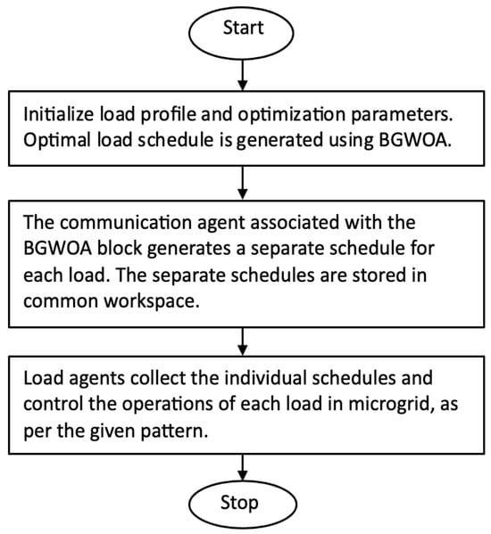
Figure 2.
Flow chart of the working MAS.
3.2. Microgrid Model for the Proposed System
The optimized schedule received from the BGWO was applied and tested in the microgrid developed in the Simulink environment, as shown in Figure 3. The major components include the following:
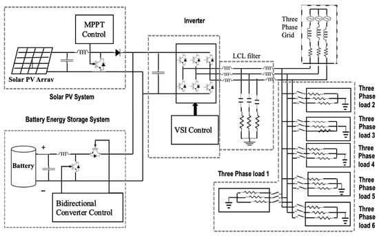
Figure 3.
Microgrid simulation model.
3.2.1. Solar Photovoltaic System
The solar PV system was designed to achieve a maximum output of 12 kW. Signal Builder was employed to generate a solar irradiance input profile that emulates real-world temporal variations observed under typical operating conditions. The temporal profile of solar irradiance is presented in Figure 4. Maximum power point tracking (MPPT) based on irradiance was used to trap the maximum power from the PV system [34]. A boost converter was used to condition the DC voltage received at 240 V to 720 V, where 720 V is the desired DC link voltage suitable for the conversion to an AC voltage of 415 V. Figure 5 illustrates the simulation results of the solar PV system, including the voltage, current, power output, and DC-link voltage characteristics.
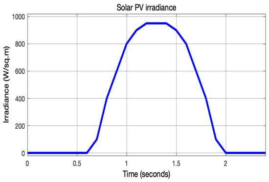
Figure 4.
Solar irradiance in . Simulation time was scaled such that 0.1 s represents 1 h of real-world time. Therefore, the interval from 0.1 to 2.4 s corresponds to a 24-h period.
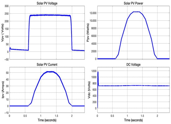
Figure 5.
Solar PV voltage, current, power, and DC link voltage.
3.2.2. Battery Energy Storage System (BESS)
The BESS was realized using a lithium-ion battery model in Simulink. The desired nominal voltage of the battery was 380 V, with an ampere capacity of 500 Ah. The chosen battery parameters were used to satisfy the load modeled in the microgrid. Batteries are a significant cost component in energy systems. Controlling degradation minimizes maintenance and replacement costs, leading to better lifecycle economics.
The primary methods employed to mitigate battery degradation included state of charge (SoC) management and temperature regulation. Temperature was actively maintained within an optimal range to minimize thermal stress on the battery. SoC management involved restricting the depth of charge and discharge cycles by maintaining the SoC between 20 and 80. This approach effectively reduced electrochemical stress, thereby prolonging battery lifespan and ensuring reliable operation.
3.2.3. Loads
The loads were modeled as AC-resistive loads with a maximum demand limit () at any point in time of less than or equal to 20 kW. is one of the constraints set by the utility to control load demand in the DSM problem. The loads were connected through switches to facilitate ON and OFF according to the schedule pattern received. The load parameters used are as shown in Table 1.
3.3. Microgrid Test Environment
Solar energy is used to reduce dependency on nonrenewable sources of energy. Solar energy can be produced more easily than other renewable energy resources (RERs). It is a widely available power source with zero carbon emissions. The solar energy was converted into electrical energy using solar photovoltaic arrays. The MPPT technique based on irradiance [34] was used to extract the maximum power from the solar PV array [35,36].
The solar PV array was connected to the point of common coupling using a boost converter and voltage source converter. The boost converter enabled the voltage of the solar PV array to match the desired DC link voltage. A battery was used in conjunction with a solar PV array to support the load during cloudy days and night time, ensuring a continuous power supply. The excess generated solar PV power was stored in the battery for later use [37,38]. This method decoupled the electricity generation from the demand. To achieve a DC link voltage of 720 V, the battery was connected through a bidirectional converter [39]. The grid-tied solar microgrid operated in current control mode [40]. The simulation parameters of solar PV are available in Table 2.
Table 2.
Solar PV/BESS simulation parameters.
The system parameters of the microgrid are shown in Table 3. Six resistive AC loads were connected in parallel to validate the scheduling scenario. A schematic diagram of the microgrid design is shown in Figure 3.
Table 3.
Microgrid system parameters.
3.4. Binary Grey Wolf Optimization (BGWO)
The grey wolf optimization (GWO) algorithm, developed by Mirjalili and colleagues in 2014 [22], is a recently introduced metaheuristic optimization technique. It is inspired by the leadership hierarchy and hunting behavior of grey wolves in nature.
The DSM problem is an MILP, where the solution takes discrete values, like 0, 1, or 2. The value 0 indicates the OFF position of the load. The value 1 indicates the ON position of the load using power from the utility. The value 2 states that the load is ON with PV/BESS power. The discrete nature of the problem restricts the search space to 0, 1, or 2. BGWOA is implemented using a sigmoid transformation to handle this binary format.
In the problem considered, six loads required scheduling for 24 h. The the solution matrix had to be a dimension of 6 × 24. The ON and OFF status of the at time t was generated using the following equation:
where and are random numbers distributed between [0, 1]. The probable solution matrix is that which satisfies the constraints (Equations (5)–(7)) discussed in Section 2. Probable solution matrices were considered the wolves (search agents) in this problem. The solution space was a multidimensional array of probable solution matrices, as shown in Figure 6. The pseudo-code to detail the working of BGWOA is given as Algorithm 1.
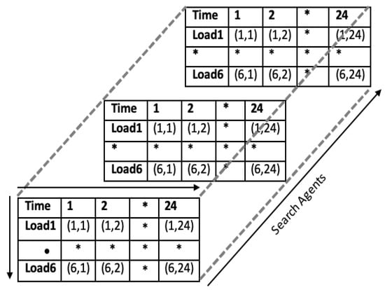
Figure 6.
Multidimensional array of search agents. The figure provides a visual representation of the candidate solutions of BGWOA. The symbols * and • are used to denote truncated entries in the 6 × 24 matrix representation, indicating that not all elements are explicitly shown.
The optimization parameters (like electricity tariff, load parameters, priority factor, inconvenience factor, incentive factor etc.), total number of search agents, and maximum number of iterations were initialized. The search agents satisfying the constraints were randomly generated, and the fitness of all search agents generated was calculated. The , , were identified amongst the search agents, and the new position of each search agent concerning the , , and search agents was calculated and updated using the a, A, and C parameters. was then calculated. Finally, the solution was chosen to be the search agent with the lowest cost.
| Algorithm1: Binary Grey Wolf Optimization Algorithm |
|
4. Results and Discussion
4.1. Binary Grey Wolf Optimization Algorithm (BGWOA) vs. Mixed Integer Linear Programming (MILP)
The objective of the demand-side management problem is to minimize the energy consumption cost from the utility grid. The load parameters used for the simulation study are given in Table 4. However, to compare the performance of BGWOA and MILP, the load parameters provided in Table 1 and Table 4 were used.
Table 4.
Load parameters.
BGWOA calculates the optimized load scheduling pattern (i.e., time slots) by considering load parameters, optimization parameters, and constraints. The optimized schedule minimizes the energy consumption cost while satisfying all system constraints and operational parameters. To validate the performance of BGWOA, MILP was used as a benchmark, as it guarantees convergence to the global minimum and is widely accepted for comparative evaluation.
As shown in Table 5, both optimization algorithms achieved the same optimal fitness value for the objective function defined in Equation (2) in Section 2 of this paper. The optimal time slots obtained were also identical, except for the case of loads 5 and 2. With reference to Table 1, the time slot 10–13 is prefered to 14–17, as it resulted in less delay while maintaining the same tariff rate for load 5. In the case of load 2, the optimal slot 11–14 is better than 12–15, as it resulted in lower delay.
Table 5.
Comparison of BGWOA and MILP with the load parameters given in Table 1.
Table 6 presents the comparative results of BGWOA and MILP obtained using the load parameters provided in Table 4. In the results, the optimal fitness value obtained using MILP is 1303; however, the operation of Load 4 was interrupted violating its atomicity in order to minimize the electricity cost. As uninterrupted operation is essential for the loads considered, the result cannot be deemed acceptable for the intended use case. At the same time, the BGWO algorithm achieved the global minimum and preserved the uninterrupted operation of all scheduled loads. These findings highlight the appropriateness of BGWOA as a candidate for further investigation and application in load scheduling problems.
Table 6.
Comparison of BGWOA and MILP with load parameters given in Table 4.
In MILP, constraints related to the dimensions of matrices play a crucial role in the solution process. Not all problems can be readily formulated and solved using MILP to obtain a global optimum. Due to this constraint, the objective functions defined by Equations (4) through (7) could not be effectively solved using the MILP approach.
Table 1 and Table 4 were compared in terms of average hourly power consumption and production, as presented in Table 7. The analysis indicates that the average energy consumption consistently exceeded the available generation capacity, thereby increasing the complexity of the optimization problem and necessitating more effective load scheduling strategies. The variation in the values of , , , and accounts for the distinct operational characteristics represented in the second table. As a result, the load parameters from Table 4 were selected for further evaluation.
4.2. Analysis of the Objective Function
This section analyzes how the defined objective function achieved the optimization goal described in Section 2.2.1, with supporting results presented in tabular form. The detailed analysis began with Equation (2) and proceeded through Equations (3) and (4), concluding with Equation (8).
Equations (2) and (3) were analyzed comparatively to determine the influence of load priority constraints on the optimization results. The results are tabulated in Table 8. For comparative analysis, initially, the priority of all the loads was set to 2. When all loads were assigned equal priority, the scheduling behaved as though no priority constraints had been applied. The resultant optimized time slots are presented in Column 4 of Table 8. The oriority assigned for each load is given in Column 5. The values in Coulmn 6 demonstrate that incorporating priority of loads into the objective function ensured that high-priority loads did not experience delays. For instance, load 2, when given the same priority factor as the other loads, began execution at time slot 10. However, with a priority factor of 1, it started at time slot 8. High-priority loads were allocated to the earliest possible time slots. Similarly, load 4 also commenced execution without any delay.
Table 8.
Comparative analysis of optimization results from Equations (2) and (3) to evaluate the impact of load priority constraints.
Table 9 illustrates the effect of the objective function defined in Equation (4). By adding a delay term to the objective function, low-priority loads no longer had to wait until the end of the operational range. As shown in Column 6 of Table 8, without the delay factor, load 1 started at time slot 10, load 3 at slot 13, and load 6 at slot 10. However, after incorporating the delay factor, optimal time slots were achieved with reduced delays, as read from Column 4 of Table 9. Load 1 started at time slot 9 instead of 10, load 3 at slot 12 instead of 13, and load 6 at slot 7 instead of 10. Thus, the delay factor ensured that no load experienced excessive delays.
Table 9.
Optimization outcomes with the load-specific delay constraint applied, as per Equation (4).
The incentive factor included in the objective function was to minimize the use of peak time slots when determining the optimal scheduling pattern. Consumers were offered an incentive of Rs 2/kW for shifting their loads from peak to off-peak time slots. Thus, comparing the results in Column 5 of Table 9 and Column 4 of Table 10, all loads except load 2 avoided peak time slots in the operational schedule. Load 2, however, was assigned high priority, so it began at the earliest available time slot. According to the KSEB tariff, peak time slots are from 6 to 8 and 18 to 22, normal tariff slots from 9 to 17, and off-peak slots from 12 to 5 and 23 to 24.
Table 10.
Final optimized scheduling results considering all objectives defined in Equation (8).
4.3. Analysis Using Different Simulation Scenarios
The optimization of load scheduling was carried out in three different scenarios as outlined below.
- Optimizing the energy consumption cost using grid power.
- Optimizing the energy consumption cost utilizing solar PV power and grid power.
- Optimizing the energy consumption cost utilizing solar PV power/BESS and grid power.
4.3.1. Optimizing the Energy Consumption Cost Using Grid Power
In this scenario, the optimization was carried out by considering
- the load parameters;
- the ToD tariff from Kerala State Electricity Board (KSEB).
As per the ToD tariff of KSEB, the 24-h day was segmented into three distinct time zones based on the utility’s load demand.
- Peak time zone;
- Normal time zone;
- Off-peak time zone.
Time slots 1–5 fell within the off-peak zone, offering the lowest electricity costs. The peak load time zones, with the highest electricity costs, occurred between time slots 6–8 and 18–22. Meanwhile, the normal time zone spanned from time slots 9–17, with electricity costs positioned between those of the low and high time zones. Figure 7 presents the ToD tariff structure of grid power in rupees for the respective time zones.
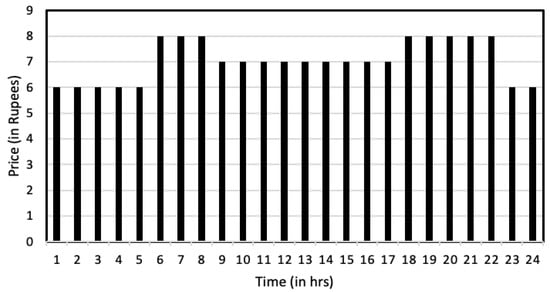
Figure 7.
ToD tariff of grid power.
Figure 8 illustrates the convergence of BGWOA using grid power. The vertical axis represents the optimal fitness values obtained with varying numbers of search agents during optimization. When 250 search agents were used, the optimal fitness value reached 1254. With five search agents, the optimal fitness was 1284, which decreased to 1279 with 10 search agents and further to 1264 with 15 search agents. Notably, the optimal fitness achieved with 45 search agents was the same as that with 250 search agents, both yielding a value of 1254. The graph indicates that an optimal number of search agents increases the likelihood of the algorithm converging to a global minimum.
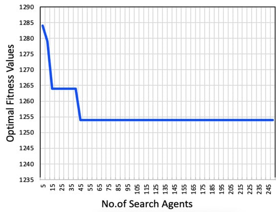
Figure 8.
BGWOA convergence graph using grid power.
Figure 9 presents a graphical representation of the expected operation schedule, also referred to as the baseline schedule, for all six loads. Figure 10 depicts the optimal load schedule obtained using BGWOA. A tabular representation is given in Table 10. The horizontal axis represents the 24-h time horizon, while the vertical axis indicates the power sources. In this case, all loads were supplied by grid power, with source 1 representing the grid and source 2 denoting PV power. The graph clearly illustrates the optimal operation schedule for all six loads with no noncritical loads operating during the peak time. The simulation results of the same are given in Figure 11.
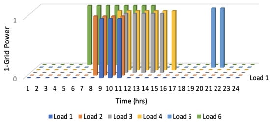
Figure 9.
Baseline schedule of all 6 loads.
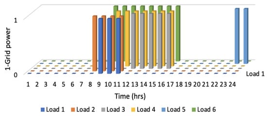
Figure 10.
BGWOA-optimized load pattern using grid power. Grid power is represented as source 1.
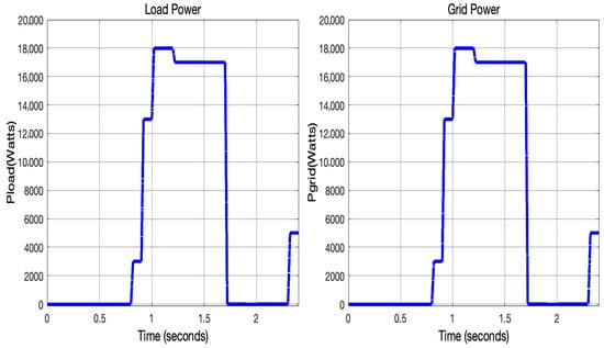
Figure 11.
Total power demand of household loads and corresponding energy consumption from the grid over a 24-h period.
4.3.2. Optimizing the Energy Consumption Cost Utilizing Solar PV Power and Grid Power
In the second scenario, both solar PV power and grid power were utilized for optimization. The maximum power generated by the solar PV array was 12 kW, provided in Table 2. For the simulation study, real-time irradiance data were sourced from SOLARMAN Smart APP, intelligent energy management application for global users (used by customers with rooftop solar PV systems), and the corresponding pattern was generated using Signal Builder. A plot of the solar PV power generated over 24 h is shown in Figure 12.
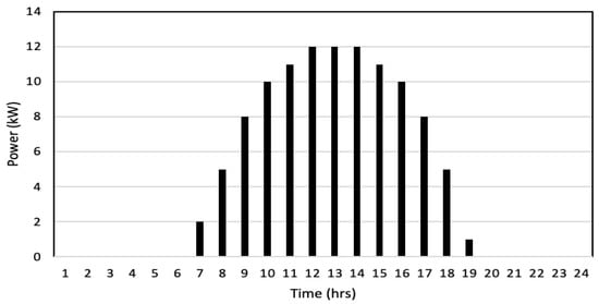
Figure 12.
Solar PV array power generated in 24 h.
Whenever solar power is unavailable, grid power is used to meet the load demand, with grid power serving as a backup source. The excess power generated by the solar PV array can be exported to the utility grid, and the KSEB as per the Kerala state electricity regulatory commission reimburses the customers at a nominal rate of Rs 3.15/- per unit. Here, in this study, we used Rs 5/per kW as the tariff rate for solar PV generated power. The combined grid tariff and PV power cost form the tariff structure was used for optimization, as shown in Figure 13. From 12 midnight to 6 a.m., and from 8 p.m. to 12 midnight, solar power was not available, so the grid tariff applied during these periods. From 7 a.m. to 7 p.m., when solar PV power was available, the cost of PV power (Rs 5/per kW) was used as the applicable tariff; otherwise, the grid tariff was considered.
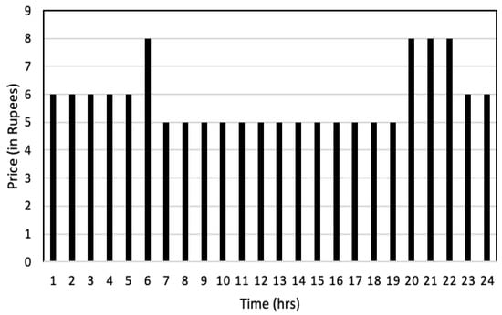
Figure 13.
Tariff structure for combined PV and grid power.
In addition to scenario 1, the optimization parameters also included the PV power generated over 24 h. Figure 14 illustrates the convergence of BGWOA using both PV and grid power. The vertical axis represents the optimal fitness values obtained with varying numbers of search agents used for optimization. With 250 search agents, the optimal fitness value for the objective function was 1168. The optimal fitness with five search agents was 1182, which decreased to 1178 with 10 search agents, and further dropped to 1173 with 15 search agents. The optimal fitness values obtained with 45 and 250 search agents were the same—1168. This suggests that as the number of search agents increased, the optimal fitness value decreased, leading to a more efficient schedule for load operation. Since the tariff rates for PV power were lower than the grid tariff, the optimal fitness value was also lower.
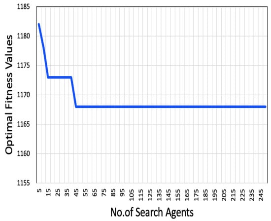
Figure 14.
BGWOA convergence plot with PV and grid power.
The loads were supplied based on the availability of PV power. As shown in Figure 15, load 2 was powered by PV power, except during time slot 9. Similarly, load 6 was supplied by both PV and grid power. The output generated by BGWOA for the second scenario included load status values of 0, 1, and 2. A status of 0 indicates the load is “off,” status 1 means the load is “on using grid power,” and status 2 signifies the load is “on using PV power.” The tabulated details can be understood by reading Table 4 and Table 10 and Figure 13. It can be noted that the majority of loads were distributed when solar power was most abundant. Notably, load 6 was moved from its 9–16 grid power schedule to 10–16. At 10, solar power was 3 kW higher than at 9. Thus, BGWOA also ensured optimal load scheduling in this scenario.
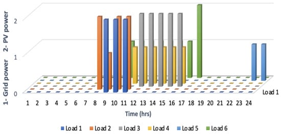
Figure 15.
Optimized load pattern using PV power and grid power.
Figure 16 illustrates the total power demand of household loads and corresponding energy supply by the grid and solar PV over a 24-h period.
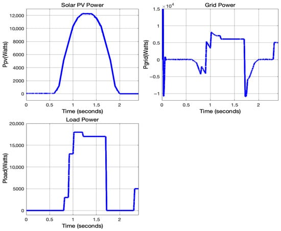
Figure 16.
24-h profile of the total household load demand and energy contribution from both grid and solar PV sources.
4.3.3. Energy Consumption Cost Utilizing Solar PV Power/BESS and Grid Power
The third scenario can be viewed as an extension of the second scenario, where PV power and BESS complement each other in meeting the load demands. Grid power was utilized as a backup whenever PV/BESS power was unavailable or not sufficient. Consequently, the tariff structure was reduced to the cost of PV power when the entire load was supplied by PV/BESS for the entire day.
As can be seen in Figure 17, the maximum production from PV was approximately 12 kW. The combined power supplied by PV and the battery to the microgrid was limited to 10 kW. The remaining energy was used to charge the battery. Hence, whenever the load power exceeded 10 kW, the excess power wascatered by the grid. At 8 and 9, the load power was less than 10 kW. From 10 to 16, the load power was greater than 10 kW. The same can also be seen in Figure 18. At time slots 10–16, the grid power took a positive value as power was drawn from the grid. At all other time slots, the excess power was supplied to the grid. Looking at the plot of the battery, it is clear that excess energy generated from time slots 10–16 was used to charge the battery.
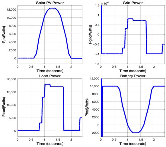
Figure 17.
24-h profile of the total household load demand and the energy contribution from the grid, solar PV system, and battery energy storage.
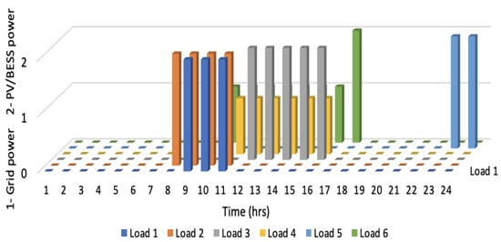
Figure 18.
Optimal load schedule using PV/BESS power and grid power.
Thus, it is proved that integrating renewable energy resources along with battery storage is a good method to achieve self-dependency in the energy management of households [40].
Table 11 shows the total electricity cost incurred while operating the optimal schedule generated, as well as the baseline schedule with the grid and grid PV tariffs. The graph in Figure 19 shows that the baseline schedule exceeded the maximum demand limit of 20 kW at time slot 11. The electricity cost was computed using Equation (3), which quantifies the cost based on the load profile and applicable tariff rates. The optimized load schedule demonstrates a strategic shift of demand away from peak tariff periods, with load operations predominantly aligned to time slots featuring higher solar power availability. Thus, the result proves that a BGWOA-based optimal schedule reduces the energy cost for consumers while considering user preferences and the utilization of power from renewable energy resources.
Table 11.
Comparison of the electricity cost (in rupees) incurred while using grid and grid PV tariffs.
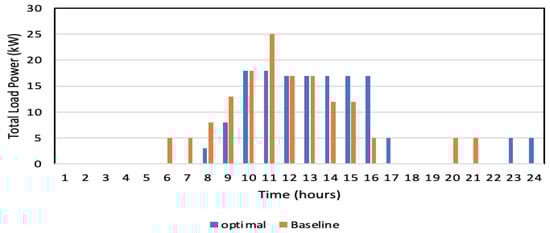
Figure 19.
Baseline vs. optimal schedule.
5. Limitations and Future Work
The proposed DSM framework is well-suited for deployment in residential microgrids equipped with advanced metering infrastructure (AMI).
Practically, the system can
- schedule controllable appliances during off-peak hours or during PV-surplus generation windows;
- react to price signals and user preferences;
- enable local control with fail-safe fallback to user-preferred baseline schedules in case of agent failure or communication breakdown;
- reduce operational costs for consumers and alleviate peak demand stress on the utility side, promoting grid stability.
However, its limitations should also be acknowledged.
First, the system was validated using only six household loads, which may not fully reflect the scalability challenges encountered in real-world residential or community microgrids. Future work will focus on incorporating real-time energy management into residential microgrids, as discussed in [41], to enhance robustness under severe environmental fluctuations. In addition, the study [42] presents an AI-based method for managing clusters of residential microgrids to reduce energy costs, maintain occupant comfort, and prevent equipment overloads. In future multi-microgrid systems, a pricing mechanism that simultaneously incentivizes both producers and consumers to actively participate in scheduling will be more effective [43]. Building on these insights, we plan to extend the MAS architecture to accommodate a larger number of controllable loads by adopting hierarchical or layered control strategies to address scalability and reduce computational overheads. Second, fault tolerance in the event of communication agent failure was not fully addressed. While fallback to a baseline schedule was implemented, more robust distributed coordination methods and fault-handling mechanisms will be explored in future work to ensure system resilience. Finally, while BGWOA was selected based on its proven efficiency, a comparative analysis with other metaheuristic techniques, such as particle swarm optimization (PSO) and genetic algorithms (GAs), based on key performance indicators (KPIs) [44], was not within the scope of this work. Such benchmarking will be addressed in future studies to provide a comprehensive evaluation of algorithmic performance in DSM applications.
6. Conclusions
In this study, a cost-optimized demand-side management framework was developed using the binary grey wolf optimization Algorithm (BGWOA) and deployed through a multi-agent system (MAS) for real-time load scheduling in residential microgrids. The simulation results across three practical scenarios demonstrated the effectiveness of the proposed approach. Notably, the optimized load schedules achieved up to a 27% reduction in electricity costs compared to the baseline operation, with approximately 65% of controllable loads shifted away from peak tariff periods. The integration of solar PV and battery storage further enhanced system performance, maintaining the lowest cost operation in scenario 3. The study demonstrated the significance and adaptability of BGWOA in load scheduling applications. A unified, cost-based multi-objective function was formulated to incorporate user preferences (priority and delay), ToD tariffs, and incentives—all expressed in monetary terms, thereby eliminating the need for normalization or weighting. The successful integration of BGWOA within a real-time MAS architecture, modeled in Stateflow, demonstrates the feasibility and real-world applicability of the proposed DSM framework for smart residential microgrids.
Author Contributions
S.V. performed the methodology implementation, programming, data aquisition and analysis, and result analysis. P.R.K. helped with the manuscript writing, document preparation, and result interpretation. E.A.J. contributed to the conceptualization and computing analysis. All authors have read and agreed to the published version of the manuscript.
Funding
This research received no external funding.
Data Availability Statement
The original contributions presented in this study are included in the article. Further inquiries can be directed to the corresponding author.
Conflicts of Interest
The authors declare no conflicts of interest.
Abbreviations
The following abbreviations are used in this manuscript:
| MAS | Multi-agent system |
| DSM | Demand-side management |
| BGWOA | Binary grey wolf optimization algorithm |
| ToD | Time-of-day |
| SDG | Sustainable development goals |
| PV | Photovoltaic |
| BESS | Batery energy storage system |
| RER | Renewable energy resource |
| DER | Distributed energy resource |
| DR | Demand response |
| MILP | Mixed-integer linear programming |
| PSO | Particle swarm optimization |
| GA | Genetic algorithm |
| ToU | Time-of-use |
| CPP | Critical peak pricing |
| RTP | Real-time pricing |
| KSEB | Kerala State Electricity Board |
| GWO | Grey wolf optimization |
| MMG | Multi-microgrid |
References
- Tamasiga, P.; Chetty, K.; Chattopadhyay, D.; Robinson, D.; Kenny, P. Empowering Communities Beyond Wires: Renewable Energy Microgrids and the Impacts on Energy Poverty and Socio-Economic Outcomes. Energy Rep. 2024, 12, 4475–4488. [Google Scholar] [CrossRef]
- Bhattacharyya, S.C. Energy access programs and sustainable development: A critical review and analysis. Energy Sustain. Dev. 2012, 16, 260–271. [Google Scholar] [CrossRef]
- UN-Habitat. World Cities Report 2020: The Value of Sustainable Urbanization; United Nations Human Settlements Programme: Nairobi, Kenya, 2020. [Google Scholar]
- Butt, O.M.; Zulqarnain, M.; Butt, T.M. Recent advancement in smart grid technology: Future prospects in the electrical power network. Ain Shams Eng. J. 2021, 12, 687–695. [Google Scholar] [CrossRef]
- Alotaibi, I.; Abido, M.A.; Khalid, M.; Savkin, A.V. A comprehensive review of recent advances in smart grids: A sustainable future with renewable energy resources. Energies 2020, 13, 6269. [Google Scholar] [CrossRef]
- Shaukat, N.; Islam, M.R.; Rahman, M.M.; Khan, B.; Ullah, B.; Ali, S.M.; Fekih, A. Decentralized, democratized, and decarbonized future electric power distribution grids: A survey on the paradigm shift from the conventional power system to microgrid structures. IEEE Access 2023, 11, 60957–60987. [Google Scholar] [CrossRef]
- Amin, S.M.; Wollenberg, B.F. Toward a smart grid: Power delivery for the 21st century. IEEE Power Energy Mag. 2005, 3, 34–41. [Google Scholar] [CrossRef]
- Rahbar, K.; Xu, J.; Zhang, R. Real-time energy storage management for renewable integration in microgrid: An off-line optimization approach. IEEE Trans. Smart Grid 2015, 6, 124–134. [Google Scholar] [CrossRef]
- Zafar, R.; Mahmood, A.; Razzaq, S.; Ali, W.; Naeem, U.; Shehzad, K. Prosumer based energy management and sharing in smart grid. Renew. Sustain. Energy Rev. 2018, 82, 1675–1684. [Google Scholar] [CrossRef]
- Kotilainen, K. Energy prosumers’ role in the sustainable energy system. In Affordable and Clean Energy; Springer International Publishing: Cham, Switzerland, 2019; pp. 1–14. [Google Scholar]
- Jabir, H.J.; Teh, J.; Ishak, D.; Abunima, H. Impacts of demand-side management on electrical power systems: A review. Energies 2018, 11, 1050. [Google Scholar] [CrossRef]
- Zeng, P.; Xu, J.; Zhu, M. Demand response strategy based on the multi-agent system and multiple-load participation. Sustainability 2024, 16, 902. [Google Scholar] [CrossRef]
- Palensky, P.; Dietrich, D. Demand side management: Demand response, intelligent energy systems, and smart loads. IEEE Trans. Ind. Inform. 2011, 7, 381–388. [Google Scholar] [CrossRef]
- Strbac, G. Demand side management: Benefits and challenges. Energy Policy 2008, 36, 4419–4426. [Google Scholar] [CrossRef]
- Haider, H.T.; See, O.H.; Elmenreich, W. A review of residential demand response of smart grid. Renew. Sustain. Energy Rev. 2016, 59, 166–178. [Google Scholar] [CrossRef]
- Bradac, Z.; Kaczmarczyk, V.; Fiedler, P. Optimal scheduling of domestic appliances via MILP. Energies 2014, 8, 217–232. [Google Scholar] [CrossRef]
- Logenthiran, T.; Srinivasan, D.; Shun, T.Z. Multi-agent system for demand side management in smart grid. In Proceedings of the 2011 IEEE Ninth International Conference on Power Electronics and Drive Systems (PEDS), Singapore, 5–8 December 2011; pp. 938–943. [Google Scholar]
- Remani, T.; Jasmin, E.A.; Imthias Ahamed, T.P. Residential load scheduling with renewable generation in the smart grid: A reinforcement learning approach. IEEE Syst. J. 2018, 13, 3283–3294. [Google Scholar] [CrossRef]
- Remani, T.; Jasmin, E.A.; Imthias Ahamed, T.P. Load scheduling with maximum demand using binary particle swarm optimization. In Proceedings of the 2015 International Conference on Technological Advancements in Power and Energy (TAP Energy), Kollam, India, 10–12 December 2015; pp. 1–5. [Google Scholar] [CrossRef]
- Kamboj, V.K.; Bath, S.K.; Dhillon, J.S. Solution of non-convex economic load dispatch problem using Grey Wolf Optimizer. Neural Comput. Appl. 2016, 27, 1301–1316. [Google Scholar] [CrossRef]
- Gupta, S.; Deep, K. An efficient grey wolf optimizer with opposition-based learning and chaotic local search for integer and mixed-integer optimization problems. Arab. J. Sci. Eng. 2019, 44, 7277–7296. [Google Scholar] [CrossRef]
- Mirjalili, S.; Mirjalili, S.M.; Lewis, A. Grey wolf optimizer. Adv. Eng. Softw. 2014, 69, 46–61. [Google Scholar] [CrossRef]
- Ayub, S.; Ayob, S.M.; Tan, C.W.; Arif, S.M.; Taimoor, M.; Aziz, L.; Bukar, A.L.; Al-Tashi, Q.; Ayop, R. Multi-Criteria Energy Management with Preference Induced Load Scheduling Using Grey Wolf Optimizer. Sustainability 2023, 15, 957. [Google Scholar] [CrossRef]
- Khan, A.R.; Mahmood, A.; Safdar, A.; Khan, Z.A.; Khan, N. Load forecasting, dynamic pricing and DSM in smart grid: A review. Renew. Sustain. Energy Rev. 2016, 54, 1311–1322. [Google Scholar] [CrossRef]
- Areekkara, S.; Kumar, R.; Bansal, R.C. An intelligent multi agent based approach for autonomous energy management in a microgrid. Electr. Power Compon. Syst. 2021, 49, 18–31. [Google Scholar] [CrossRef]
- Pipattanasomporn, M.; Feroze, H.; Rahman, S. Multi-agent systems in a distributed smart grid: Design and implementation. In Proceedings of the 2009 IEEE/PES Power Systems Conference and Exposition (PSCE), Seattle, WA, USA, 15–18 March 2009; pp. 1–8. [Google Scholar] [CrossRef]
- Kerala State Electricity Board Limited. Tariff at a Glance. 3 November 2023. Available online: https://www.kseb.in/updates (accessed on 15 June 2025).
- Ahamed, T.P.I.; Maqbool, S.D.; Malik, N.H. A reinforcement learning approach to demand response. In Proceedings of the Centenary Conference of Electrical Engineering, Bangalore, India, 15–17 December 2011; pp. 168–172. [Google Scholar]
- Javadi, M.S.; Askarzadeh, A.; Siano, P.; Mohammadi-Ivatloo, B. Self-scheduling model for home energy management systems considering the end-users discomfort index within price-based demand response programs. Sustain. Cities Soc. 2021, 68, 102792. [Google Scholar] [CrossRef]
- Rezaee Jordehi, A. Enhanced leader particle swarm optimisation (ELPSO): A new algorithm for optimal scheduling of home appliances in demand response programs. Artif. Intell. Rev. 2020, 53, 2043–2073. [Google Scholar] [CrossRef]
- Setlhaolo, D.; Xia, X.; Zhang, J. Optimal scheduling of household appliances for demand response. Electr. Power Syst. Res. 2014, 116, 24–28. [Google Scholar] [CrossRef]
- Bahlke, F.; Liu, Y.; Pesavento, M. Stochastic load scheduling for risk-limiting economic dispatch in smart microgrids. In Proceedings of the 2016 IEEE International Conference on Acoustics, Speech and Signal Processing (ICASSP), Shanghai, China, 20–25 March 2016; pp. 3121–3125. [Google Scholar] [CrossRef]
- Collins, M.E.; Silversides, R.W.; Green, T.C. Multi-agent system control and coordination of an electrical network. In Proceedings of the Universities Power Engineering Conference (UPEC), London, UK, 4–7 September 2012; pp. 1–5. [Google Scholar]
- Anjali, M.; Jasmin, E.A. Control of grid-tied solar battery system with irradiance-based MPPT. In Proceedings of the International Conference on Intelligent Solutions for Smart Grids and Smart Cities, Singapore, 21–23 September 2022; Springer Nature: Singapore, 2022; pp. 1–9. [Google Scholar]
- Subudhi, B.; Pradhan, R. A comparative study on maximum power point tracking techniques for photovoltaic power systems. IEEE Trans. Sustain. Energy 2013, 4, 89–98. [Google Scholar] [CrossRef]
- De Brito, M.A.G.; Sampaio, L.P.; de Azevedo e Melo, G.; Canesin, C.A. Evaluation of the main MPPT techniques for photovoltaic applications. IEEE Trans. Ind. Electron. 2013, 60, 1156–1167. [Google Scholar] [CrossRef]
- Kabir, M.N.; Mishra, Y.; Ledwich, G.; Dong, Z.Y.; Wong, K.P. Coordinated control of grid-connected photovoltaic reactive power and battery energy storage systems to improve the voltage profile of a residential distribution feeder. IEEE Trans. Ind. Inform. 2014, 10, 967–977. [Google Scholar] [CrossRef]
- Omran, W.A.; Kazerani, M.; Salama, M.M.A. Investigation of methods for reduction of power fluctuations generated from large grid-connected photovoltaic systems. IEEE Trans. Energy Convers. 2011, 26, 318–327. [Google Scholar] [CrossRef]
- Ponnaluri, S.; Khan, M.S.A.; Kumar, B.R. Comparison of single and two stage topologies for interface of BESS or fuel cell system using the ABB standard power electronics building blocks. In Proceedings of the 2005 European Conference on Power Electronics and Applications, Dresden, Germany, 11–14 September 2005; pp. 1–10. [Google Scholar]
- Mbungu, N.T.; Abu-Mahfouz, A.M.; Hancke, G.P.; Isaac, S.J. A dynamic energy management system using smart metering. Appl. Energy 2020, 280, 115990. [Google Scholar] [CrossRef]
- Wang, C.; Xiong, R.; Zhang, Y.; Zhao, H.; Cao, J. Prioritized Sum-Tree Experience Replay TD3 DRL-Based Online Energy Management of a Residential Microgrid. Appl. Energy 2024, 368, 123471. [Google Scholar] [CrossRef]
- Wang, C.; Wang, M.; Wang, A.; Zhang, X.; Zhang, J.; Ma, H.; Yang, N.; Zhao, Z.; Lai, C.S.; Lai, L.L. Multiagent Deep Reinforcement Learning-Based Cooperative Optimal Operation with Strong Scalability for Residential Microgrid Clusters. Energy 2025, 314, 134165. [Google Scholar] [CrossRef]
- Wang, C.; Liu, Y.; Zhang, Y.; Xi, L.; Yang, N.; Zhao, Z.; Lai, C.S.; Lai, L.L. Strategy for Optimizing the Bidirectional Time-of-Use Electricity Price in Multi-Microgrids Coupled with Multilevel Games. Energy 2025, 323, 135731. [Google Scholar] [CrossRef]
- Alrashed, S. Key performance indicators for Smart Campus and Microgrid. Sustain. Cities Soc. 2020, 60, 102264. [Google Scholar] [CrossRef]


Disclaimer/Publisher’s Note: The statements, opinions and data contained in all publications are solely those of the individual author(s) and contributor(s) and not of MDPI and/or the editor(s). MDPI and/or the editor(s) disclaim responsibility for any injury to people or property resulting from any ideas, methods, instructions or products referred to in the content. |
© 2025 by the authors. Licensee MDPI, Basel, Switzerland. This article is an open access article distributed under the terms and conditions of the Creative Commons Attribution (CC BY) license (https://creativecommons.org/licenses/by/4.0/).