Transient Voltage Stability Analysis of the Dual-Source DC Power System

Abstract

This paper analyzes the transient voltage stability of the dual-source DC power system. The system’s equivalent model is first established. Subsequently, the effect mechanisms of line parameters and voltage-source rectifiers’ current control inner loops on the system’s transient voltage instability are investigated. It indicates that these factors reduce the power supply capacity of the source, increasing the risk of transient instability in the system. Then, considering the influence of fault depths, the influence of different large disturbances on the transient voltage stability is investigated. Furthermore, the critical cutting voltage and critical cutting time for DC power systems are determined and then validated on the MATLAB R2023b/Simulink platform. Finally, based on the mixed potential function theory, the impact of system parameter variations on stability boundaries is analyzed quantitatively. Simulation verification is conducted on the MATLAB R2023b/Simulink platform, and experimental verification is conducted on the RT-LAB Hardware-in-the-Loop platform. The results of the quantitative analysis and experiments corroborate the conclusions drawn from the mechanistic analysis, underscoring the critical role of line parameters and converter control parameters in the system’s transient voltage stability.

1. Introduction

With the rapid development of power electronic technology and increasing popularity of renewable distributed generators, DC power systems incorporating more than one power source, as illustrated in Figure 1, have attracted significant research attention [1,2,3,4,5]. Various applications, including more-electric aircraft, marine vessels, commercial buildings, and electric vehicles, have adopted DC power distribution systems. Renewable sources such as wind power are often connected to the DC grid through the VSR to participate in energy supply [6,7,8,9].

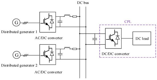
Figure 1. Typical structure of a dual-source DC power system.

However, the power electronic converters on the load side always behave as CPLs, whose NIR characteristics destabilize the DC power system [10,11,12,13]. For a CPL, the voltage variation occurs inversely to the current change. When large disturbances such as abrupt load increases or short-circuit failures occur, the NIR characteristics may induce a power imbalance during the transient process, consequently leading to bus voltage oscillations [14]. To improve the efficiency of power transmission, ensuring the bus voltage stability is the primary goal of DC power system operation. Therefore, it is crucial to investigate physical mechanisms underlying voltage instability during transient processes and identify the key parameters and system segments that predominantly influence stability.

The nonlinear characteristics of the DC power systems are strongly revealed when a large perturbation occurs. To analyze stability characteristics and depict operating trajectories, nonlinear quantities are typically linearized through time-domain analysis, after which the asymptotically stable region is constructed according to the system’s equilibrium points [15,16,17]. In Refs. [15,17], several classic transient analysis methods are applied, and the influence of circuit parameters on the stable region is illustrated. But the specific expression of the stable boundary is unknown. Ref. [16] discusses large-signal analysis methods available to DC power systems with CPLs but omits critical components such as current control loops. The principle of these methods is based on constructing energy functions using Lyapunov’s second method. However, the Lyapunov function-based stability analysis method cannot provide an algebraic expression of the system’s stability region and thus fails to visually demonstrate the impact of parameters on transient stability [18]. In contrast, the mixed potential method can directly construct mathematical expressions of the system’s stability boundary, thereby providing explicit guidance for parameter design of the system [19,20]. Table 1 summarizes the commonly used transient stability analysis methods and presents their advantages and disadvantages. By comparison, it can be seen that the mixed potential function method is a suitable analysis method for high-order nonlinear systems.

Table 1. Comparison of various transient stability analysis methods.

Method	Advantages	Limitations
Time-domain simulation methods [21]	The analysis results are reliable and accurate. Suitable for various nonlinear systems. The complete time-domain and frequency-domain characteristics of the system are retained.	For high-order nonlinear systems, the calculation process is complex and time-consuming.
TS fuzzy modeling methods [14,15,21]	The influence of the system’s physical and control dynamics on the stability domain can be revealed. Can be extended to high-order systems.	Obtained regions of attraction are conservative. The more nonlinear variables in the system, the more computationally complex the analysis is.
Mixed potential function methods [19,20,22]	The stability criterion can be obtained in mathematical form. High compatibility. The physical interpretation of the energy function is well-defined.	If only the circuit structure is taken into consideration when constructing the mixed potential function, the stability boundaries obtained are conservative.
Sum-of-squares programming methods [23,24]	Less conservative.	Higher orders make it computationally intractable due to the large scale of the semi-definite programming problem to be solved.
Inverse trajectory methods [25,26,27]	Accurately depict the attraction domain of power systems and achieve visualization.	Only applicable to low-order power systems.

As for the mechanistic analysis, most studies focus on the transient stability of AC power systems [28,29,30,31], where instability mechanisms are characterized using P-δ curves. On the basis of the extended equal-area criterion, these references reveal that the reason for the transient angle instability is the mismatch between the acceleration area and the deceleration area, causing the generator rotor to accelerate and be unable to stop. Based on this theoretical foundation, control methods for enhancing the transient stability of AC power systems were proposed in Refs. [28,31], while a unique index for evaluating system transient stability was developed in Ref. [30]. The revelation of instability mechanisms holds significant implications for advancing stability research. However, the research on instability mechanisms of DC power systems is insufficient. In addition, DC power systems generally do not consider synchronous generators and have no rotational inertia, so the analysis method based on P-δ curves is not applicable. Early work in [32] proposed a stability criterion for VSC-based DC power grids based on the principle of equal electric quantity. However, this approach neglects the impact of line parameters and source converters’ current control inner loops, which play critical roles in determining system transient dynamics. Moreover, the transient behavior of the system under different disturbance types or fault depths has not been investigated sufficiently. Therefore, existing studies on the instability mechanisms in DC power systems are insufficient, highlighting the need for more in-depth research in this field.

Considering line parameters and dynamic responses of VSRs’ current control inner loops, the transient voltage stability of the dual-source DC power system is investigated to address the limitations of prior studies. The main contributions of this paper are as follows:

(1)

The source–load interaction characteristics of the system are represented intuitively based on the equivalent system model derived through equivalence transformation of the VSR’s control structure and circuit configuration, thereby revealing the essential requirements for stable operation. On the basis of stable operating requirements, the critical cutting voltage and critical cutting time when different large disturbances occur can be determined under ideal conditions, which is further validated through MATLAB/Simulink simulations.

(2)

Transient voltage instability mechanisms are investigated considering line parameters and current inner-loop control parameters of VSRs. Under different large disturbances (e.g., abrupt load increases or short-circuit faults with varying depths), the influence of system parameters on the source power supply capacity is discussed, revealing the system’s dynamic characteristics during transient processes.

(3)

The stability criterion and boundaries of the system are revealed based on the mixed potential theory. In accordance with Lyapunov’s third theorem on stability, the impact of crucial parameters on transient voltage stability is analyzed and verified through MATLAB/Simulink simulations and experiments. The obtained results provide valuable guidance for the design of system parameters.

This paper is organized as follows: The topology and equivalent model of the dual-source DC power system are analyzed in Section 2. In Section 3, the operational characteristics of the source and the load under various large disturbances are investigated, revealing instability mechanisms. Section 4 estimates the system’s critical cutting voltage and critical cutting time during different transient processes, and verifies the effectiveness of this determination method in MATLAB/Simulink. Thereafter, the impact of parameters on stabilizing boundaries is quantified using the mixed potential function method in Section 5. To verify the theoretical analysis, in Section 6, the simulation model of the dual-source DC power system is constructed, and experiments are carried out on the RTLAB platforms. Finally, the conclusions are summarized in Section 7.

2. Topology and Modeling of the Dual-Source DC Power System

This section introduces the construction and mathematical model of the dual-source DC power system. By employing the pole-zero cancelation method, the current control loop of the VSR is simplified to an equivalent first-order inertial model. In this way, while maintaining the dynamic performance of control loops, the source-side converter can be simplified to a controlled current source. Meanwhile, the load-side converter is typically equivalent to a CPL. Then, the equivalent model of the dual-source power system is established.

2.1. Topology and Control of the Dual-Source DC Power System

Figure 2 illustrates the topology of the dual-source DC power system investigated in this paper. The system consists of two VSRs, DC-side capacitance (C₁, C₂ and C_s), line resistance (R₁ and R₂), line inductance (L₁ and L₂), and a CPL. In DC power systems, the constant-voltage-controlled converter and its terminal load can typically be modeled as a CPL. Two VSRs provide stable and continuous electrical energy for the load, improving the system’s stability.

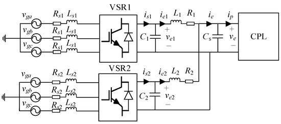
Figure 2. The topology of the dual-source DC power system.

Unlike master–slave control that requires communication links for power distribution, DC droop control facilitates autonomous power sharing among parallel VSRs using only local voltage measurements, thereby eliminating communication dependencies [33]. In the dual-source DC system investigated, the droop control strategy is adopted to enhance reliability and simplify system architecture by removing the need for a centralized communication network. And the current inner loop with PI control structures is adopted to enhance the response speed of the control system. Therefore, as shown in Figure 3, the control strategy of VSR1 is primarily based on a dual-loop structure. The control structure of VSR2 is consistent with that of VSR1. In this case, the bus voltage of the system remains constant in stable operation.

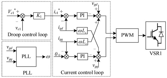
Figure 3. The control blocking of VSR1.

2.2. Modeling of the Dual-Source DC Power System

As derived in reference [34], the current inner loops in VSRs can be simplified as the first-order model W_ci [14]. VSRs investigated in this paper can be equated to voltage-controlled current sources with the expression shown in (1).

$$\left\{\begin{array}{l}{i}_{s1}=K_1(V_{e1}^{*}-v_{e1})W_{ci1}\\ i_{s2}=K_2(V_{e2}^{*}-v_{e2})W_{ci2}\end{array}\right.$$

(1)

where i_s1 is the output current of VSR1, and i_s2 is the output current of VSR2. K₁ and K₂ represent the droop coefficients of VSR1 and VSR2, respectively. V_e1^* and V_e2^* denote the reference output voltages of VSR1 and VSR2, respectively. v_e1 and v_e2 are output voltages of VSR1 and VSR2. W_ci1 and W_ci2 represent the first-order models of VSR1 and VSR2, respectively. And W_ci1 and W_ci1 can be calculated by (2).

$$\left\{\begin{array}{l}{W}_{ci1}={\displaystyle \frac{1}{1+s{T}_1}}\\ W_{ci2}={\displaystyle \frac{1}{1+s{T}_2}}\end{array}\right.$$

(2)

where T₁ and T₂ denote the inertial time constants of current control loops in VSR1 and VSR2, respectively. T₁ and T₂ can be calculated by (3).

$$\left\{\begin{array}{l}{T}_1={\displaystyle \frac{L_{s1}}{k_{pi1}{K}_{PWM1}}}={\displaystyle \frac{R_{s1}}{k_{ii1}{K}_{PWM1}}}\\ T_2={\displaystyle \frac{L_{s2}}{k_{pi2}{K}_{PWM2}}}={\displaystyle \frac{R_{s2}}{k_{ii2}{K}_{PWM2}}}\end{array}\right.$$

(3)

where L_s1 and L_s2 represent the AC grid inductance of VSR1 and VSR2, respectively. R_s1 and R_s2 denote the AC grid resistance of VSR1 and VSR2, respectively. k_pi1 and k_ii1 are the proportional and integral coefficients of the current controller in VSR1. k_pi2 and k_ii2 are the proportional and integral coefficients of the current controller in VSR2. K_PWM1 and K_PWM2 are the gains of PWM in VSR1 and VSR2.

Equation (4) is the large-signal model of a CPL. The transmission line model is represented by a Π-type lumped parameter equivalent circuit [35]. In this case, the effects of line capacity and resonance phenomena are ignored. The distributed capacitance is integrated into the DC-link capacitors (C₁, C₂, and C_s) at both terminals of the transmission line. Thus, only the line inductance and resistance parameters are retained. In addition, the impact of limiters and over-modulation in VSRs is not considered. Figure 4 demonstrates the equivalent circuit of the dual-source DC power system, and the parameter explanation along with their initial values are listed in Table 2.

$$i_p={\displaystyle \frac{P_s}{v_e}}$$

(4)

where P_s is the load power of the CPL, and v_e denotes the bus voltage of the system.

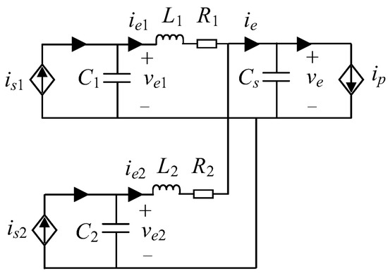
Figure 4. The equivalent circuit of the dual-source DC power system.

Table 2. Control and circuit parameters of the dual-source DC power system.

Items	Symbols	Values
Line resistance	R1, R2	0.3 Ω, 1 Ω
Line inductance	L1, L2	3 mH, 3 mH
DC-side capacitance of CPL	Cs	1.5 mF
DC-side capacitance of VSR1	C1	4.3 mF
DC-side capacitance of VSR2	C2	4.3 mF
Droop control coefficient of VSR1	K1	0.8
Droop control coefficient of VSR2	K2	0.5
Reference voltage of VSR1	Ve1*	650
Reference voltage of VSR2	Ve2*	700
Inertial time constant of the current control loop in VSR1	T1	15 × 10−5
Inertial time constant of the current control loop in VSR2	T2	21 × 10−5
Grid inductance	Ls1, Ls2	2 mH, 2 mH
Grid resistance	Rs1, Rs2	0.1 Ω, 0.1 Ω
Grid voltage	vg	311 V
Grid angular frequency	w	314 rad/s

According to the circuit illustrated in Figure 4, the state equations of the dual-source DC power system can be expressed as follows:

$$\left\{\begin{array}{l}{T}_1{\displaystyle \frac{d{i}_{s1}}{dt}}+i_{s1}=(V_{e1}^{*}-v_{e1})K_1\\ T_2{\displaystyle \frac{d{i}_{s2}}{dt}}+i_{s2}=(V_{e2}^{*}-v_{e2})K_2\\ C_1{\displaystyle \frac{d{v}_{e1}}{dt}}=i_{s1}-i_{e1}\\ C_2{\displaystyle \frac{d{v}_{e2}}{dt}}=i_{s2}-i_{e2}\\ v_{e1}=v_e+R_1{i}_{e1}+L_1{\displaystyle \frac{d{i}_{e1}}{dt}}\\ v_{e2}=v_e+R_2{i}_{e2}+L_2{\displaystyle \frac{d{i}_{e2}}{dt}}\\ C_s{\displaystyle \frac{d{v}_e}{dt}}=i_{e1}+i_{e2}-i_p\end{array}\right.$$

(5)

where C₁ is the DC-side capacitance of VSR1, C₂ is the DC-side capacitance of VSR2, and C_s is the DC-side capacitance of CPL. i_e1 is the current flowing through the branch containing L₁ and R₁, and i_e2 is the current flowing through the branch containing L₂ and R₂.

3. Transient Voltage Instability Mechanisms Considering System Parameters

Based on the model built in Section 2, operational characteristics and essential stable operating requirements of the dual-source DC power system are revealed in this section. Compared with previous works, the influence of line parameters and current control inner loops of VSRs on the system’s transient performance is taken into consideration. An intuitive visualization of the system’s transient voltage instability phenomena is also provided. Through researching movements of the system’s source and load characteristic curves on a two-dimensional plane diagram (v_e-i_dc) under different large disturbances, the underlying mechanisms of transient voltage instability are investigated.

3.1. Operational Characteristics and Requirements for Stable Operations

According to (5), the operational characteristics of the system can be modeled as

$$\left\{\begin{array}{l}{i}_e=A-{\displaystyle \frac{(R_2+R_1)v_e}{R_1{R}_2}}\\ C_s{\displaystyle \frac{d{v}_e}{dt}}=i_e-i_p\end{array}\right.$$

(6)

where i_e denotes the system’s source characteristics, i_p denotes the system’s load characteristics, v_e denotes the bus voltage of the system, and the variable A in the expression of i_e can be expressed by

$$A={\displaystyle \frac{V_{e1}^{*}}{R_1}}+{\displaystyle \frac{V_{e2}^{*}}{R_2}}-{\displaystyle \frac{i_{s1}}{R_1{K}_1}}-{\displaystyle \frac{i_{s2}}{R_2{K}_2}}-{\displaystyle \frac{T_1}{R_1{K}_1}}{\displaystyle \frac{d{i}_{s1}}{dt}}-{\displaystyle \frac{T_2}{R_2{K}_2}}{\displaystyle \frac{d{i}_{s2}}{dt}}-{\displaystyle \frac{L_1}{R_1}}{\displaystyle \frac{d{i}_{e1}}{dt}}-{\displaystyle \frac{L_2}{R_2}}{\displaystyle \frac{d{i}_{e2}}{dt}}$$

(7)

where the variable A remains constant during stable operations, while it is variable when disturbances occur. This is because all DC currents (e.g., i_e1, i_e2, i_s1 and i_s2) maintain steady-state values in stable operations, resulting in zero-valued differential terms for DC currents in the expression of A. And the VSRs’ output currents i_s1 and i_s2 are constants when the system is stable.

Figure 5a illustrates source–load interactions of the dual-source DC power system, where the source characteristic curve i_e intersects the load characteristic curve i_p at operation points S_o and S₁. The expressions of the source characteristic curve i_e and the load characteristic curve i_p are shown in (6). The corresponding bus voltages for S_o and S₁ are represented as U_o and U₁. The system’s initial bus voltage is defined as U_(to). If U_(to) > U₁, i_p > i_e means that the powersupplied by the source cannot meet the needs of the load at the initial state. So, the capacitance C_s will discharge to maintain the load need, leading v_e to drop and eventually stabilize at U₁ due to the existence of power balance at S₁ (i_p = i_e). If U₁ > U_(to) > U_o, i_p < i_e means that the power provided by the source is more than the load needs. The capacitance C_s will charge to restore the excessive power, causing v_e to rise and finally stay at U₁ as mentioned before. Thus, the operation point S₁ is defined as the stable operation point [32], which represents an equilibrium state of the system. When U_o > U_(to) > 0, i_p > i_e, the power supplied by the source cannot meet the needs of the load during the whole dynamic process, causing the discharge of C_s. The discharge of C_s reduces the value of the bus voltage, making v_e continue to drop until 0 V. Therefore, the system can be stable if U_(to) > U_o. S_o is defined as the unstable operation point, and U_o is defined as the limit operating voltage.

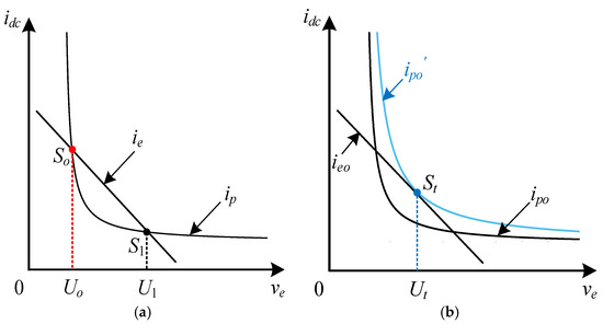
Figure 5. Operational characteristics of the dual-source DC power system. (a) Interaction between the system’s source and load. (b) Operational characteristics of the system when P_s = P_{s_max}.

The foregoing analysis yields the requirements for stable operations of the system: the source and load operating characteristic curves must share common operating points, with the initial bus voltage U_(to) during dynamic processes exceeding the limit operating point U_o. If the above requirements are satisfied, the system will stabilize at the operation point S₁, and the values of DC voltages and currents corresponding to the point S₁ are the system’s steady-state values.

Assuming the load power P_s corresponding to i_po is defined as P_so, if P_s = P_s′ (P_s′ > P_so), as shown in Figure 5b, the source curve i_eo will tangent the corresponding load characteristic curve i_po′ at the operation point S_t. The bus voltage of the operation point S_t is defined as U_t. In this case, if U_(to) > U_t, i_po′ > i_eo, the capacitance C_s will discharge to maintain the load needs, leading v_e to drop and eventually stabilize at U_t because the power equilibrium is achieved at S_t. If U_t > U_(to) > 0, i_po′ > i_eo all the time, so the discharge of C_s reduces the value of bus voltage, making v_e continue to drop until 0 V. Thus, S_t is the stable operating point as well as the unstable operation point for the system when P_s = P_s′. According to stable operation requirements, P_s′ is the maximum power P_{s_max} that the source i_eo can afford for stable operation. The values of U_t and P_{s_max} are expressed as (8). When the source characterization presents as i_eo, the load power P_s is supposed to be less than P_{s_max} for stable operations. The variable A in (8) is a constant determined by steady-state DC current values under the condition that the source characteristic behaves as i_eo. Therefore, these steady-state values vary with changes in the source characteristics i_e, resulting in differences in U_t and P_{s_max}.

$$\left\{\begin{array}{l}{U}_t={\displaystyle \frac{R_1{R}_{2}A}{2(R_1+R_2)}}\\ P_{s\_max}={\displaystyle \frac{R_1{R}_2{A}^2}{4(R_1+R_2)}}\end{array}\right.$$

(8)

3.2. Effect Mechanisms of System Parameters on the Transient Voltage Stability

In previous research, the line parameters and current inner-loop control parameters of VSRs were ignored [14,32]. In this case, the operational characteristics of the dual-source DC power system can be expressed as(9). When an abrupt increase occurs, movement trajectories of the system’s operating points can be illustrated in Figure 6a. Changes in load will alter the system’s operating states. During the transient process, the DC-side capacitor discharges to meet the load requirements, causing v_e to decrease and the load-side current value to increase. Therefore, after the disturbance occurs, the load operating point will move from point S₁ on the i_p curve to point S₂ on the i_p’ curve, and the source operating point will move along the i_ef curve from point S₁ to point S₂. Operating point S₂ is the new stable operating point. Under the above disturbance, the method discussed in previous works can obtain a new equilibrium state of the system and achieve transient voltage stability.

$$\left\{\begin{array}{l}{i}_{ef}=V_{e1}^{*}{K}_1+V_{e2}^{*}{K}_2-(K_1+K_2)v_e\\ (C_s+C_1+C_2){\displaystyle \frac{d{v}_e}{dt}}=i_{ef}-i_p\end{array}\right.$$

(9)

where i_ef denotes the source characteristics ignoring line parameters and current inner-loop control parameters of VSRs.

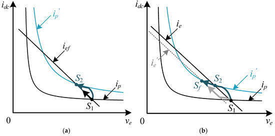
Figure 6. Transient operational characteristics of the dual-source DC power system. (a) Transient operational characteristics without line parameters and VSRs’ current control inner loops. (b) Transient operational characteristics with line parameters and VSRs’ current control inner loops.

However, the aforementioned analysis is overly idealistic. In practical power systems, the influence of line parameters on stability is typically non-negligible. Moreover, for VSRs employing dual closed-loop control, the current inner loop governs the system’s dynamic response performance and further affects the source operating characteristics during transient processes. Therefore, the combined impact of line parameters and the current inner loops on the system’s operational behavior is investigated. The operational characteristics of the dual-source DC power system can thus be expressed as (6).

Unlike previous works, the value of A reduces under the same large disturbance due to the rise in DC currents (e.g., i_e1, i_e2, i_s1 and i_s2) and differential terms for DC currents, as derived from (7). It results in a downward shift of the source characteristic curve post-disturbance, as illustrated in Figure 6b. The trajectories of the system’s operating points are depicted as follows: The source operation point transitions from point S₁ on curve i_e to S_f on curve i_e′, while the load operating point moves from S₁ on curve i_p to S_f on curve i_p′. Here, S_f is the new stable operating point for the dual-source DC power system, considering line parameters and current inner loops in VSRs. Under the new equilibrium state represented by the point S_f, the value of v_e is lower, while the DC currents exhibit higher magnitudes. Moreover, a more severe disturbance may eliminate common operating points between the source and load characteristic curves, as a larger power supply–demand mismatch leads to further increases in values and differential terms for DC currents. Overall, when considering line parameters and current inner loops of VSRs, the source’s supply capability is reduced, leading to deteriorated transient stability of the system. In extreme conditions, a greater disparity between power supply and demand results in a higher rate of rise in DC-side currents, which further diminishes the source’s supply capacity.

3.3. Influence of Different Large Disturbances on the Transient Voltage Stability

3.3.1. Abrupt Load Increases

Load failures are usually manifested as abrupt increases in the load power. In Figure 7, when an abrupt load increase occurs, i_p moves to i_p″. In this scenario, the requirements for stable operations of the system cannot be satisfied. The power imbalance between the source and load sharply increases the load-side current while reducing v_e. Simultaneously, due to the discharge of C₁ and C₂, v_e1 and v_e2 decrease while i_e1 and i_e2 increase. Consequently, the variable A in (6) experiences a sudden decline, shifting the source characteristic curve from i_e to i_e″. This process exacerbates the source–load imbalance, ultimately driving v_e to collapse rapidly to 0 V.

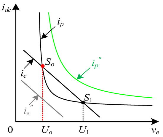
Figure 7. Changes in the system’s operation characteristics after an abrupt load increase.

However, during the transient process, the value of A varies due to DC current fluctuations (e.g., i_e1, i_e2, i_s1 and i_s2) and the presence of DC current differential terms. As demonstrated in (7), increasing the reference voltages (V_e1^* and V_e2^*) and droop coefficients (K₁ and K₂) or decreasing inertial time constants of the current control loop (T₁ and T₂) and line inductance-to-resistance ratio (L₁/R₁ and L₂/R₂) is beneficial for the system’s transient voltage stability.

3.3.2. Short-Circuit Failures

In the event of a short-circuit failure on the DC bus, as shown in Figure 8, the system’s load characteristics i_pc manifest as (10).

$$i_{pc}=i_p+i_L={\displaystyle \frac{P_s}{v_e}}+{\displaystyle \frac{v_e}{R_f}}$$

(10)

where R_f denotes the short-circuit resistance, and i_L is the short-circuit current.

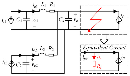
Figure 8. Equivalent circuit of the dual-source DC power system with a short-circuit failure.

The operational characteristics of the system under short-circuit failures are shown in Figure 9. The load curve is represented as i_pc (where R_f = R_f1 and P_s = P_o). A-value decreases during the transient process, shifting the source characteristic curve i_e to i_ec. In this case, the stable operation requirements are satisfied, so the system will finally work stably at S_c1. Figure 9a illustrates the influence mechanisms of fault depth variations on the transient stability. Systems with different short-circuit resistances exhibit different operating characteristics: A reduction in short-circuit resistance leads to a more significant power imbalance. When R_f = R_f2, i_p changes to i_pc1, the source characteristic curve i_e moves to i_ec′ due to a heavier reduction in A. No common operation points exist, and the system will collapse rapidly. In Figure 9b, given a fixed short-circuit resistance R_f1, post-disturbance systems show the following: An increase in P_s leads to a more significant power imbalance. For P_s = P_{s_c}′, i_p changes to i_pc2 and the source curve i_e moves to i_ec″ due to the heavier reduction in A. No common operation points for i_pc2 and i_ec″ exist, so the system will be unstable post-disturbance.

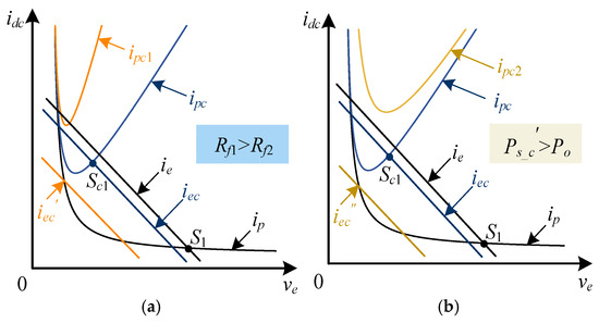
Figure 9. Operational characteristics of the dual-source DC power system with short-circuit failures. (a) Operational characteristics with different fault depths. (b) Operational characteristics with different P_s values.

In a word, the system can operate at a new equilibrium point if the post-disturbance conditions satisfy stable operation requirements. Otherwise, the system collapse will occur.

4. Determination of Critical Cutting Voltage for the Dual-Source DC Power System

Timely elimination of large disturbances is crucial for restoring power system stability. For DC power systems, two types of large disturbances are investigated in this paper: abrupt load increase and bus short-circuit failure.

The transient operating characteristics of the system are shown in Figure 10, where the line parameters and time constants of the current inner loop of source converters are ignored. Under these conditions, the source characteristic curve i_ef maintains a constant position despite large disturbances. At the initial state, the source curve i_ef intersects the load curve i_p at operating points S_o and S₁. In Figure 10a, i_p shifts to i_pf under an abrupt load increase. Provided that the fault is cleared before the bus voltage drops to U_o, the load operating point moves from curve i_pf to curve i_p, and i_p > i_ef at this moment. Finally, excess electricity is stored in DC capacitors and the bus voltage v_e stabilizes at U₁, where i_ef = i_p. Thus, the system returns to the initial steady state. For the short-circuit failure situation shown in Figure 10b, by the same reasoning, it can be concluded that as long as the fault is cleared before the bus voltage drops to U_o, the system can return to the initial steady state. We define the system’s critical cutting voltage as U_c. Therefore, U_c = U_o, which can be calculated by (11). The critical cutting time for DC power systems is defined as the time interval between the fault inception and the instant when the bus voltage drops to U_c, which is represented as t_c.

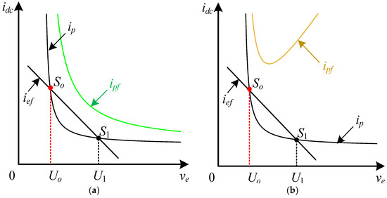
Figure 10. Transient operational characteristics of the system under different large disturbances. (a) Transient operational characteristics with an abrupt load increase. (b) Transient operational characteristics with a short-circuit failure.

Compared with post-fault AC power systems, DC power systems generally do not contain synchronous generators and have no rotational inertia. Therefore, when calculating U_c and t_c, only the dynamic variations in the DC-side capacitor current need to be considered, while the critical clearing time of AC power systems is generally calculated by the iterative method due to the dynamic behavior of second-order components [36].

$$U_c={\displaystyle \frac{\left(V_{e1}^{*}{K}_1+V_{e2}^{*}{K}_2\right)-\sqrt{{\left(V_{e1}^{*}{K}_1+V_{e2}^{*}{K}_2\right)}^2-4P_{so}\left(K_1+K_2\right)}}{2\left(K_1+K_2\right)}}$$

(11)

where P_so denotes the initial load power.

To validate the above analysis for U_c and t_c, a dual-source DC power system model is built in MATLAB/Simulink, with system parameters listed in Table 2. P_so = 140 kW and U_c is derived from (11). In the abrupt load increase case, there is an abrupt increase in P_s at 1.0 s. As illustrated in Figure 11, when a disturbance occurs, the bus voltage v_e recovers to U₁ if the overload is shed before v_e drops below U_c. Conversely, failure to shed the excessive load in a timely manner results in v_e collapsing to 0 V. In the short-circuit failure case, R_f = 0.01 Ω and the short-circuit failure occurs at 1.0 s. The experimental results are presented in Figure 12. Stable operation can be restored by promptly clearing the faulted line before v_e drops to U_c. It is noteworthy that during a short-circuit fault, the fault must be cleared within a microsecond-level time frame to maintain system stability, which imposes stringent requirements on circuit breakers.

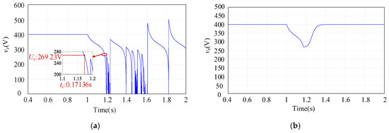
Figure 11. The bus voltage curve after an abrupt load increase: (a) 0 ≤ U_c < U_o; (b) U_c ≥ U_o.

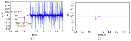
Figure 12. The bus voltage curve after a short-circuit failure: (a) 0 ≤ U_c < U_o; (b) U_c ≥ U_o.

5. Stability Analysis of the Dual-Source DC Power System Based on the Mixed Potential Function Method

This section constructs the mixed potential function of the system for quantifying the effects of parameters on transient voltage stability. Based on Lyapunov’s third stability theorem, the stability criterion and boundary of the system can be derived, guiding the parameter design to improve system stability.

5.1. Mixed Potential Function Construction for the System

Based on the inductors, capacitors, and non-energy-storage elements in the circuit, the mixed potential function of the system can be established, which is expressed as

$$P(\mathit{i},\mathit{v})={\displaystyle \int {\displaystyle \sum _{\mu >r+s}{v}_{\mu }}}d{i}_{\mu }+{\displaystyle \sum _{\delta =r+1}^{r+s}{i}_{\delta }{v}_{\delta }}$$

(12)

where i and v are vectors of all inductance currents and capacitance voltages in the circuit, respectively. v_μ is the voltage of non-storage element μ, and i_μ is its current. v_δ is the voltage of capacitance δ, and i_δ is its current. μ represents the non-storage element branch, and δ denotes the capacitance branch. r is the number of inductance branches in the system, and s is the number of capacitance branches in the system.

Uniform expression for the mixed potential function is

$$P(\mathit{i},\mathit{v})=-A(\mathit{i})+B(\mathit{v})+(\mathit{i},\mathit{\gamma }\mathit{v}-\mathit{\alpha })$$

(13)

where A(i) is the current potential function, and B(v) is the voltage potential function. γ is the constant matrix related to the circuit structure, and α is a constant vector.

Since T₁ and T₂ are extremely small, W_ci1 and W_ci2 can be approximated as the constant 1. Based on the equivalent system structure illustrated in Figure 4, the current potential function of non-storage elements in the dual-source DC power system can be derived as

$$\begin{array}{ll}\hfill {\displaystyle {\int }_{\Gamma }{\displaystyle \sum _{\mu >r+s}{v}_{\mu }}}d{i}_{\mu }& ={\displaystyle {\int }_0^{(V_{e1}^{*}-v_{e1})K_1}[V_{e1}^{*}-(V_{e1}^{*}-v_{e1})K_1/K_1]d[(V_{e1}^{*}-v_{e1})K_1]}\\ & +{\displaystyle {\int }_0^{(V_{e2}^{*}-v_{e2})K_2}[V_{e2}^{*}-(V_{e2}^{*}-v_{e2})K_2/K_2]d[(V_{e2}^{*}-v_{e2})K_2]}\\ & -{\displaystyle {\int }_0^{i_{e1}}{R}_1{i}_{e1}d{i}_{e1}}-{\displaystyle {\int }_0^{i_{e2}}{R}_2{i}_{e2}d{i}_{e2}}-{\displaystyle {\int }_0^{i_s}\frac{P_s}{i_s}d{i}_s}\end{array}$$

(14)

Total capacitance energy is calculated as

$${\displaystyle \sum _{\delta =r+1}^{r+s}{i}_{\delta }{v}_{\delta }}{|}_{\Gamma }=-v_{e1}[(V_{e1}^{*}-v_{e1})K_1-i_{e1}]-v_{e2}[(V_{e2}^{*}-v_{e2})K_2-i_{e2}]-v_e(i_{e1}+i_{e2}-i_s)$$

(15)

By combining (14) and (15), the mixed potential function of the system can be derived and expressed in the form of (13) as follows:

$$\begin{array}{ll}\hfill P(\mathit{i},\mathit{v})=& \underset{-A_1(i)}{\underbrace{-{\displaystyle \frac{R_1{i}_{e1}^2}{2}}}}\underset{-A_2(i)}{\underbrace{-{\displaystyle \frac{R_2{i}_{e2}^2}{2}}}}+\underset{B_1(v)}{\underbrace{{\displaystyle \frac{K_1{v}_{e1}^2}{2}}-K_1{V}_{e1}^{*}{v}_{e1}}}+\underset{B_2(v)}{\underbrace{{\displaystyle \frac{K_2{v}_{e2}^2}{2}}-K_2{V}_{e2}^{*}{v}_{e2}}}\\ & +\underset{B_3(v)}{\underbrace{{\displaystyle {\int }_0^{v_e}\frac{P_s}{v_e}}d{v}_e}}+{\left[\begin{array}{l}{i}_{e1}\\ i_{e2}\end{array}\right]}^T\left[\begin{array}{l}1 0 -1\\ 0 1 -1\end{array}\right] \left[\begin{array}{l}{v}_{e1}\\ v_{e2}\\ v_e\end{array}\right]\end{array}$$

(16)

5.2. Stability Criterion and Boundary Analysis for the System

According to Lyapunov’s third stability theorem, when all i and v values in the circuit satisfy (17) and the system satisfies the condition (18), the system is still able to operate at a stable equilibrium after a large disturbance. According to Lyapunov’s third theorem on stability, the system is guaranteed to converge to a stable equilibrium point after a large disturbance if the following conditions are met: (1) all current i and voltage v values in the circuit satisfy (17); (2) the system fulfills condition (18) as |i| + |v| → ∞ [19,20].

$$\left\{\begin{array}{l}{\mu }_1=\min {\lambda }_i(L^{-1/2}{A}_{ii}{L}^{-1/2})\\ {\mu }_2=\min {\lambda }_v(C^{-1/2}{B}_{vv}{C}^{-1/2})\\ {\mu }_1+{\mu }_2>0\end{array}\right.$$

(17)

where A_ii and B_vv can be calculated by (19).

$$\left\{\begin{array}{l}{P}_i={\displaystyle \frac{\partial P(\mathit{i},\mathit{v})}{\partial i}}\\ P_v={\displaystyle \frac{\partial P(\mathit{i},\mathit{v})}{\partial v}}\\ P^{*}(i,v)={\displaystyle \frac{{\mu }_1-{\mu }_2}{2}}P(i,v)+{\displaystyle \frac{1}{2}}(P_i,L^{-1}{P}_i)+{\displaystyle \frac{1}{2}}(P_v,C^{-1}{P}_v)\to \infty \end{array}\right.$$

(18)

$$\left\{\begin{array}{l}{A}_{ii}={\displaystyle \frac{{\partial }^{2}A(i)}{\partial i^2}}\\ B_{vv}={\displaystyle \frac{{\partial }^{2}B(v)}{\partial v^2}}\end{array}\right.$$

(19)

Based on (17), the eigenvalues of the system can be represented as

$$\left\{\begin{array}{l}{\lambda }_{i1}=R_1/L_1\\ {\lambda }_{i2}=R_2/L_2\\ {\lambda }_{v1}=K_1/C_1\\ {\lambda }_{v2}=K_2/C_2\\ {\lambda }_{v3}=-P_s/(C_s{v}_e^2)\end{array}\right.$$

(20)

Combining (17) and (20), the large-signal criterion of the system is

$$\min \left\{{\displaystyle \frac{R_1}{L_1}}-{\displaystyle \frac{P_s}{C_s{v}_e^2}},{\displaystyle \frac{R_2}{L_2}}-{\displaystyle \frac{P_s}{C_s{v}_e^2}}\right\}>0$$

(21)

Based on (21), it can be concluded that the transient voltage stability of the system is dependent on line parameters R₁, L₁, and C_s, as well as the load power P_s and the bus voltage v_e. As demonstrated in (5), the value of bus voltage v_e is influenced by parameters such as K, T, and V_e^* in the VSRs.

We set the parameter values as shown in Table 2. R₁/L₁ < R₂/L₂, and the stability criterion of the system is obtained by (22). Combined with transient values of v_e in the simulation, the stability boundary P_lim can be calculated. The original stability boundary P_limo = 44.88 kW. As illustrated in Table 3, we vary some parameters in Table 2 to validate the effects of parameters on the stability boundaries of the system while leaving other parameters unchanged. The system’s stability boundary can also be modified by adjusting control loop parameters (K, T, and V_e^*) in the dual-source DC power system due to their influences on the transient value of v_e.

$${\displaystyle \frac{R_1}{L_1}}-{\displaystyle \frac{P_s}{C_s{v}_e^2}}>0$$

(22)

Table 3. The stability boundary of the dual-source DC power system (R₁/L₁ < R₂/L₂).

Changed Parameters	Transient Value of ve	Value of Plim
R1 = 0.2 Ω, L1 = 5 mH	550 V	18.15 kW
Ve1* = 660 V, Ve2* = 710 V	564 V	47.71 kW
K1 = 1, K2 = 0.8	592 V	52.57 kW
Cs = 1 mF	552 V	30.47 kW
T1 = 3 × 10−3, T2 = 15 × 10−3	500 V	37.5 kW

Assuming R₂ = 0.1 Ω, R₂/L₂ < R₁/L₁, and the stability criterion of the system is obtained by (23). We set other parameter values as shown in Table 2, it can be derived that the original stability boundary P_limo′ = 13.78 kW. As illustrated in Table 4, we vary some parameters in Table 1 to validate the effects of parameters on the stability boundaries of the system, while leaving others unchanged.

$${\displaystyle \frac{R_2}{L_2}}-{\displaystyle \frac{P_s}{C_s{v}_e^2}}>0$$

(23)

Table 4. The stability boundary of the dual-source DC power system (R₂/L₂ < R₁/L₁).

Changed Parameters	Transient Value of ve	Value of Plim
R2 = 0.05 Ω, L2 = 5 mH	526 V	4.15 kW
Ve1* = 655 V, Ve2* = 705 V	530 V	14.05 kW
K1 = 0.9, K2 = 0.6	577 V	16.65 kW
Cs = 1 mF	515 V	8.84 kW
T1 = 3 × 10−3, T2 = 15 × 10−3	470 V	11.05 kW

As demonstrated in Table 3 and Table 4, an increase in K₁ or K₂ leads to a higher P_lim, whereas an increase in T₁ or T₂ reduces P_lim. Additionally, higher values of V_e1^* or V_e2^* contribute to an expanded stability boundary of the system. Conversely, decreasing C_s, R₂/L₂ or R₁/L₁ diminishes the stability margin. These findings align with the instability mechanisms discussed in Section 3.

6. Simulation and Experimental Verification

This section verifies the theoretical analysis through simulations first. The simulation model illustrated in Figure 2 is implemented on the MATLAB/Simulink platform. We subject the load power P_s to an abrupt step change from 10 kW to 50 kW at t = 1 s. The corresponding simulation results for various test cases are presented in Figure 13. Notably, transient stability refers to a power system’s ability to maintain a new steady-state operation or restore original steady-state operation following a large disturbance [37]. When subjected to large disturbances, systems exhibiting voltage collapse with severe oscillations inherently lack stable operating points [14,15].

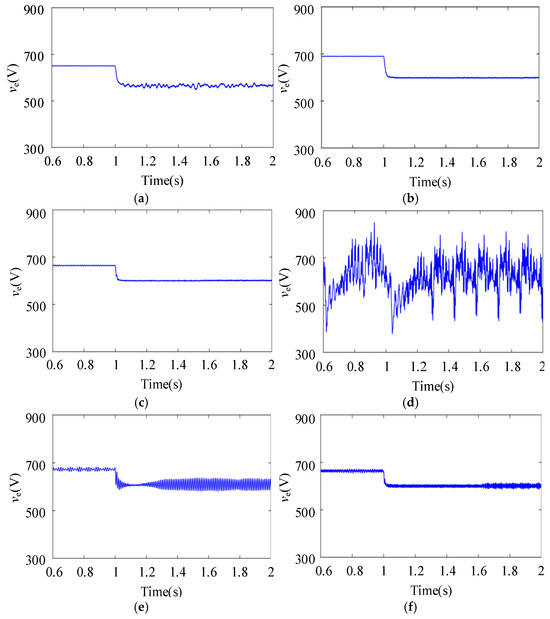
Figure 13. Simulation results of various test cases under a large disturbance. (a) Operation with the initial setting. (b) Operation with V_e1^* = 700 V and V_e2^* = 720 V. (c) Operation with K₁ = 1.2 and K₂ = 1. (d) Operation with V_e1^* = 700 V, V_e2^* = 720 V, T₁ = 15 × 10⁻³, and T₂ = 2 × 10⁻³. (e) Operation with V_e1^* = 700 V, V_e2^* = 720 V, R₁ = R₂ = 0.1 Ω, and L₁ = L₂ = 5 mH. (f) Operation with K₁ = 1.2, K₂ = 1 and C_s = 0.5 mF.

(1)

Figure 13a demonstrates the system’s transition from stable to unstable operation following an abrupt load increase, with the corresponding parameters listed in Table 2. As analyzed in Section 3.1 and supported by the P_limo calculated in Section 5.2, the system exhibits stable behavior prior to the load change, but the system will become unstable afterward because P_s exceeds the limit. The simulation results validate both the mechanistic analysis and the stability criterion.

(2)

As shown in Figure 13b, when V_e1^* increases to 700 V and V_e2^* increases to 720 V, there are no oscillations in the bus voltage v_e, and the system has reached a new stable equilibrium state. This phenomenon occurs because increasing parameter V_e1^* and V_e2^* increases the source supply’s rated voltage value A/R₁/R₂, thereby enhancing its energy delivery capability as the stability boundary P_lim expands. Increasing values of V_e1^* and V_e2^* can help the system retain the stable operation point during disturbances.

(3)

Compared to Figure 13a, in Figure 13c, increasing values of K₁ and K₂ helps the system transform to a new equilibrium point, which enhances the system’s transient voltage stability. The rationale is that increasing K₁ and K₂ effectively reduces the voltage source’s internal resistance, thereby enhancing the power delivery capacity of i_e to the load side and expanding the stability margin.

(4)

Case (d) increases T₁ and T₂ on the basis of case (b). As depicted in Figure 13d, variations in T₁ and T₂ destabilize the system. From the perspective of instability mechanisms, this phenomenon occurs because increasing parameters T₁ and T₂ reduces the source supply’s rated voltage value, consequently diminishing its energy delivery capability. In addition, the stability boundary P_lim is limited when T₁ and T₂ increase. Therefore, selecting smaller inertial time constants of current control loops is essential to ensure stable operation.

(5)

Based on case (b), reducing R₂ and R₁ while increasing L₁ and L₂ leads to bus voltage oscillations before and after a large disturbance, as shown in Figure 13e. These oscillations become more severe following the disturbance. As analyzed in Section 3.3 and based on the P_lim calculated in Section 5.2, the values of R₂/L₂ and R₁/L₁ are crucial to the transient voltage stability of the system, and decreasing the values of R₂/L₂ and R₁/L₁ will cause damage to the system stability. The simulation results exhibit agreement with the theoretical analysis.

(6)

In Figure 13f, decreasing C_s based on case (c) makes the bus voltage v_e oscillate, and the oscillations become more severe following the disturbance. This is because reducing C_s diminishes the stability limit power P_lim indicated by (21), consequently weakening the system’s disturbance rejection capability. However, the transient response of the system demonstrates significant improvement in speed.

The theoretical analysis has been further verified experimentally on the RT-LAB Hardware-in-the-Loop platform. We subject the load power P_s to an abrupt step change from 10 kW to 50 kW at t = 4 s. The experimental results are shown in Figure 14. The experimental results in Figure 14b,c demonstrate that increasing V_e1^*, V_e2^*, K₁ and K₂ indeed enhances the power supply capacity of the source end, improving the transient stability of the system. The experimental results in Figure 14d–f prove that reducing R₂/L₂, R₁/L₁ and C_s as well as increasing T₁ and T₂ have negative effects on the transient stability of the system.

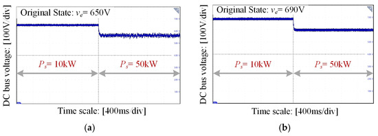
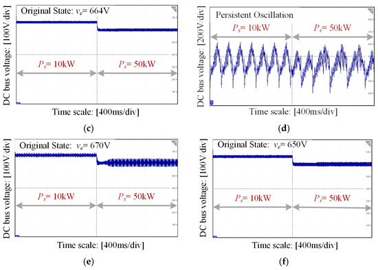
Figure 14. Experimental results of various test cases under a large disturbance. (a) Operation with the initial setting. (b) Operation with V_e1^* = 700 V and V_e2^* = 720 V. (c) Operation with K₁ = 1.2 and K₂ = 1. (d) Operation with V_e1^* = 700 V, V_e2^* = 720 V, T₁ = 15 × 10⁻³, and T₂ = 2 × 10⁻³. (e) Operation with V_e1^* = 700 V, V_e2^* = 720 V, R₁ = R₂ = 0.1 Ω, and L₁ = L₂ = 5 mH. (f) Operation with K₁ = 1.2, K₂ = 1 and C_s = 0.5 mF.

7. Conclusions

The main conclusions are as follows:

(1)

Stable operation requirements: To achieve stable operation, the source and load operating characteristic curves must share at least one common operating point, with the initial bus voltage during dynamic processes exceeding the limit operating point U_o. Under ideal conditions, the system’s critical cutting voltage is U_o when different large disturbances occur, and the critical cutting time is the time interval between the fault inception and the instant when the bus voltage drops to U_o. These results provide guidance for the fault protection.

(2)

Impact of converter control and line parameters: The line parameters and current inner-loop control parameters of VSRs reduce the power supply capacity of the source during transient processes, deteriorating the transient voltage stability of the system. When the system experiences large disturbances, such as abrupt load increases or short-circuit faults with varying depths, the transient voltage instability is fundamentally attributed to the absence of common operating points between the source and load characteristic curves, which violates the essential stability requirements. Therefore, in the design of source converter controllers, the current inner-loop inertia constant should be minimized to enhance the dynamic performance.

(3)

Crucial stability factors and design guidelines: The line resistance/inductance ratios and converter control parameters, such as the inertia constants of current control inner loops, critically influence transient voltage stability. Increasing the reference voltages, droop coefficients and DC-side capacitors, or reducing the inertial time constants of the current control loop and the line inductance-to-resistance ratios, enhances the transient voltage stability of the system. These findings offer quantitative design guidelines for optimal parameter selection in dual-source DC power systems.

(4)

Limitations and future work: However, during the transient process, the source curve is actually variable considering line parameters and the current inner-loop control dynamics. To obtain accurate U_c and t_c, it is necessary to predict the moving trajectories of the source characteristic curve i_e during the transient process. In addition, the influences of limiters and over-modulation are ignored. Further research can continue to address these deficiencies. Future work will also investigate instability mechanisms of DC power systems under multiple operational scenarios, including submarine DC power systems with pulsed power loads.

References

- Wang, T.; Li, F.; Yin, C.; Jin, G. Small Disturbance Stability Analysis of Onshore Wind Power All-DC Power Generation System Based on Impedance Method. Energies 2024, 17, 1459. [Google Scholar] [CrossRef]
- Hu, H.; Wang, X.; Peng, Y.; Xia, Y.; Yu, M.; Wei, W. Stability Analysis and Stability Enhancement Based on Virtual Harmonic Resistance for Meshed DC Distributed Power Systems with Constant Power Loads. Energies 2017, 10, 69. [Google Scholar] [CrossRef]
- Sun, K.; Yao, W.; Fang, J.; Ai, X.; Wen, J.; Cheng, S. Impedance Modeling and Stability Analysis of Grid-Connected DFIG-Based Wind Farm with a VSC-HVDC. IEEE J. Emerg. Sel. Top. Power Electron. 2020, 8, 1375–1390. [Google Scholar] [CrossRef]
- Nasirian, V.; Moayedi, S.; Davoudi, A.; Lewis, F.L. Distributed Cooperative Control of DC Microgrids. IEEE Trans. Power Electron. 2015, 30, 2288–2303. [Google Scholar] [CrossRef]
- Kunjumuhammed, L.P.; Pal, B.C.; Gupta, R.; Dyke, K.J. Stability Analysis of a PMSG-Based Large Offshore Wind Farm Connected to a VSC-HVDC. IEEE Trans. Energy Convers. 2017, 32, 1166–1176. [Google Scholar] [CrossRef]
- Zheng, L.T.; Luo, Y.B.; Fang, S.D.; Niu, T.; Chen, G.H.; Liao, R.J. Large-Signal Stability Analysis of All-Electric Ships with Integrated Energy Storage Systems. IEEE Trans. Ind. Appl. 2025. early access. [Google Scholar] [CrossRef]
- Ku, H.-K.; Park, C.-H.; Kim, J.-M. Full Simulation Modeling of All-Electric Ship with Medium Voltage DC Power System. Energies 2022, 15, 4184. [Google Scholar] [CrossRef]
- Bosich, D.; Giadrossi, G.; Pastore, S.; Sulligoi, G. Weighted Bandwidth Method for Stability Assessment of Complex DC Power Systems on Ships. Energies 2022, 15, 258. [Google Scholar] [CrossRef]
- Griffo, A.; Wang, J. Large Signal Stability Analysis of ‘More Electric’ Aircraft Power Systems with Constant Power Loads. IEEE Trans. Aerosp. Electron. Syst. 2012, 48, 477–489. [Google Scholar] [CrossRef]
- Kwasinski, A.; Onwuchekwa, C.N. Dynamic Behavior and Stabilization of DC Microgrids With Instantaneous Constant-Power Loads. IEEE Trans. Power Electron. 2011, 26, 822–834. [Google Scholar] [CrossRef]
- Chang, F.; Cui, X.; Wang, M.; Su, W.; Huang, A.Q. Large-Signal Stability Criteria in DC Power Grids with Distributed-Controlled Converters and Constant Power Loads. IEEE Trans. Smart Grid. 2020, 11, 5273–5287. [Google Scholar] [CrossRef]
- Herrera, L.; Zhang, W.; Wang, J. Stability Analysis and Controller Design of DC Microgrids with Constant Power Loads. IEEE Trans. Smart Grid. 2017, 8, 881–888. [Google Scholar]
- Belkhayat, M.; Cooley, R.; Witulski, A. Large Signal Stability Criteria for Distributed Systems with Constant Power Loads. In Proceedings of the PESC’95-Power Electronics Specialist Conference, Atlanta, GA, USA, 18–22 June 1995; Volume 2, pp. 1333–1338. [Google Scholar]
- Kim, H.; Kang, S.; Seo, G.; Jang, P.; Cho, B. Large-Signal Stability Analysis of DC Power System with Shunt Active Damper. IEEE Trans. Ind. Electron. 2016, 63, 6270–6280. [Google Scholar] [CrossRef]
- Marx, D.; Magne, P.; Nahid-Mobarakeh, B.; Pierfederici, S.; Davat, B. Large Signal Stability Analysis Tools in DC Power Systems with Constant Power Loads and Variable Power Loads—A Review. IEEE Trans. Power Electron. 2012, 27, 1773–1787. [Google Scholar] [CrossRef]
- Teng, C.P.; Wang, Y.B.; Zhou, B.K.; Wang, F.; Zhang, F.Y. Large-Signal Stability Analysis of DC Microgrid with Constant Power Loads. Trans. China Electro. Soc. 2019, 34, 973–982. [Google Scholar]
- Nie, J.T.; Zhao, Z.M.; Yuan, L.Q.; Wen, W.S.; Zhang, Y.C. Stability of Three-Phase Grid-Connected PWM Rectifier Cascaded with Constant Power Loads Based on TS Fuzzy Models. Power Syst. Technol. 2020, 44, 973–982. [Google Scholar]
- Kabalan, M.; Singh, P.; Niebur, D. Large Signal Lyapunov-Based Stability Studies in Microgrids: A Review. IEEE Trans. Smart Grid. 2017, 8, 2287–2295. [Google Scholar] [CrossRef]
- Brayton, R.K.; Moser, J.K. A Theory of Nonlinear Networks. I. Quart. Appl. Math. 1964, 22, 1–33. [Google Scholar] [CrossRef]
- Jeltsema, D.; Scherpen, J.M.A. On Brayton and Moser’s Missing Stability Theorem. IEEE Trans. Circuits Syst. II-Express Briefs 2005, 52, 550–552. [Google Scholar] [CrossRef]
- Xiong, L.S.; Liu, X.K.; Liu, Y.H.; Zhuo, F. Modeling and Stability Issues of Voltage-source Converter-dominated Power Systems: A Review. CSEE J. Power Energy Syst. 2022, 8, 1530–1549. [Google Scholar]
- Yin, H.H.; Xu, Q.M.; Zhou, X.P.; Huang, X.C.; Wang, L.; Shuai, Z.K. Large-Signal Stability Analysis of Modular Multilevel Converter Base on Mixed Potential Theory. CSEE J. Power Energy Syst. 2025, 11, 1211–1225. [Google Scholar]
- Anghel, M.; Milano, F.; Papachristodoulou, A. Algorithmic Construction of Lyapunov Functions for Power System Stability Analysis. IEEE Trans. Circuits Syst. I-Regul. Pap. 2013, 60, 2533–2546. [Google Scholar] [CrossRef]
- Meng, F.W.; Wang, D.N.; Yang, P.H.; Xie, G.Z.; Guo, F. Application of Sum-of-Squares Method in Estimation of Region of Attraction for Nonlinear Polynomial Systems. IEEE Access 2020, 8, 14234–14243. [Google Scholar] [CrossRef]
- Hu, Q.; Fu, L.J.; Ma, F.; Ji, F. Large Signal Synchronizing Instability of PLL-Based VSC Connected to Weak AC Grid. IEEE Trans. Power Syst. 2019, 34, 3220–3229. [Google Scholar] [CrossRef]
- Li, P.F.; Li, X.L.; Wang, C.S.; Guo, L.; Peng, K.; Zhang, Y.; Wang, Z. Review of Stability Analysis Model and Mechanism Research of Medium- and Low-Voltage Flexible DC Distribution System. Electr. Power Autom. Equip. 2021, 41, 3–21. [Google Scholar]
- Pan, L.; Li, X.L.; Wang, Z.; Tang, W.Q.Y.; Guo, L. Overview of Transient Stability Analysis of Phase Locked Loop Synchronization in Weak-Grid Connected VSC. Electr. Power Autom. Equip. 2023, 43, 138–151. [Google Scholar]
- Shen, C.; Shuai, Z.K.; Shen, Y.; Peng, Y.L.; Liu, X.; Li, Z.Y.; Shen, Z. Transient Stability and Current Injection Design of Paralleled Current-controlled VSCs and Virtual Synchronous Generators. IEEE Trans. Smart Grid. 2021, 12, 1118–1134. [Google Scholar] [CrossRef]
- Zhao, F.; Shuai, Z.K.; Huang, W.; Shen, Y.; Shen, Z.J.; Shen, C. A Unified Model of Voltage-Controlled Inverter for Transient Angle Stability Analysis. IEEE Trans. Power Deliv. 2022, 37, 2275–2288. [Google Scholar] [CrossRef]
- Shen, Y.; Peng, Y.L.; Shuai, Z.K.; Zhou, Q.; Zhu, L.P.; Shen, Z.J. Hierarchical Time-Series Assessment and Control for Transient Stability Enhancement in Islanded Microgrids. IEEE Trans. Smart Grid. 2023, 14, 3362–3374. [Google Scholar] [CrossRef]
- Zhao, F.; Shuai, Z.K.; Huang, W.; Peng, Y.L.; Zhou, K.; Li, R.E. Transient Stability Analysis of SG-VSG Parallel Systems Considering Mode Switching Control. CSEE J. Power Energy Syst. 2023. early access. [Google Scholar]
- Zhang, X.Y.; Shao, X.Y.; Fu, Y.; Zhao, X.Y.; Jiang, G.W. Transient Voltage Recovery Control and Stability Criterion of VSC-based DC Power Grid. IEEE Trans. Power Syst. 2021, 36, 3496–3506. [Google Scholar] [CrossRef]
- Karlsson, P. DC Distributed Power Systems-Analysis, Design and Control for a Renewable Energy System. Doctoral Thesis, LUND University, Lund, Sweden, 2002. [Google Scholar]
- Zhang, X.; Zhang, C.W. PWM Rectifiers and Their Control, 1st ed.; China Machine Press: Beijing, China, 2017; pp. 89–91. [Google Scholar]
- Ma, S.C.; Xu, B.Y.; Bo, Z.Q.; Andrew, K. The Research on Lumped Parameter Equivalent Circuit of Transmission Line. In Proceedings of the 8th International Conference on Advances in Power System Control, Operation and Management (APSCOM 2009), Hong Kong, China, 8–11 November 2009; pp. 1–5. [Google Scholar]
- Wang, G.Z.; Guo, J.B.; Ma, S.C.; Zhang, X.; Guo, Q.L.; Fan, S.X. Data-driven Transient Stability Assessment Using Sparse PMU Sampling and Online Self-check Function. CSEE J. Power Energy Syst. 2023, 9, 910–920. [Google Scholar]
- Liu, S.; Chen, C. Analysis of Energy Function for Transient Stability of Power System, 1st ed.; Science Press: Beijing, China, 2014; p. 11. [Google Scholar]
Disclaimer/Publisher’s Note: The statements, opinions and data contained in all publications are solely those of the individual author(s) and contributor(s) and not of MDPI and/or the editor(s). MDPI and/or the editor(s) disclaim responsibility for any injury to people or property resulting from any ideas, methods, instructions or products referred to in the content. |
© 2025 by the authors. Licensee MDPI, Basel, Switzerland. This article is an open access article distributed under the terms and conditions of the Creative Commons Attribution (CC BY) license (https://creativecommons.org/licenses/by/4.0/).