Cable External Breakage Source Localization Method Based on Improved Generalized Cross-Correlation Phase Transform with Multi-Sensor Fusion

Abstract

In response to the need for cable outer sound source localization, this paper proposes a collaborative localization method based on an improved generalized cross-correlation phase transform (GCC-PHAT) and multi-sensor fusion. By constructing a secondary cross-shaped sensor array model, employing a phase transform weighting function to suppress environmental noise, and incorporating an adaptive environmental compensation algorithm to eliminate multipath effects, a set of spatial localization equations is established. Innovatively, a dynamic weighting factor linked to the startup threshold is introduced; the Levenberg–Marquardt optimization algorithm is then used to iteratively solve the nonlinear equations to achieve preliminary localization in a single-pile coordinate system. Finally, a dynamic weighted fusion model is constructed through DBSCAN spatial clustering to determine the final sound source position. Experimental results demonstrate that this method reduces the mean square error of time delay estimation by 94.7% in a 90 dB industrial noise environment, decreases the localization error by 65.4% in multi-obstacle scenarios, and ultimately maintains localization accuracy within 3 m over a range of 100 m. This performance is significantly superior to that of traditional TDOA and SRP-PHAT methods, offering a high-precision localization solution for underground cable protection.

1. Introduction

With the rapid development of the social economy, urban power grids are continuously expanding, and cable lines are increasingly employed [1]. However, improper operation of construction machinery frequently leads to the excavation of underground direct-buried cables, resulting in recurrent power system failures [2]. Statistics indicate that within a span of five years, there were as many as 5000 cable failure incidents [3], posing a severe threat to cable safety. According to data from the National Energy Administration in 2024, cable failures caused by construction machinery damage accounted for 58.3% nationwide. Consequently, the establishment of an efficient damage source localization system becomes particularly critical [4,5].

In the field of sound source localization, microphone arrays have garnered significant attention globally and are increasingly adopted as the primary solution [6,7]. This technology has been highly emphasized both domestically and internationally [8], achieving notable success in automotive electronics [9], aerospace [10], and other fields. Nonetheless, existing research encounters technical limitations in cable protection scenarios. For instance, a signal strength-based positioning method exhibits an error of ±2.5 m within a 10 m range; the synchronized positioning scheme proposed in [11] is rendered ineffective by insufficient clock synchronization accuracy at engineering sites; the planar array method discussed in [12] suffers a high localization failure rate in noisy environments; and while the spherical wave sensor array introduced in [13] performs better in three-dimensional space, it requires certain preconditions. Moreover, although adaptive eigenvalue decomposition is used in [14] for simultaneous localization of multiple sound sources, its accuracy remains limited. In [15], accurate localization of outdoor sound sources is achieved, yet with varying levels of precision. For confined underground environments, the three-dimensional mapping techniques described in [16,17] present a blind zone of 8–12 m for localization, which is inadequate for direct-buried cable protection requirements.

This paper concentrates on the development of a multifaceted sound source localization system through the following research contributions. First, a quadratic cross-shaped sensor array is designed [18], and the time-delay estimation accuracy is enhanced by employing the generalized cross-correlation algorithm weighted by phase transform (GCC-PHAT), which maintains low error even under a 90 dB noise environment. Second, a dynamic weight allocation model is established to automatically down-weight sensor data when the signal strength falls below 50 dB, effectively mitigating interference from abnormal data. Finally, an LM optimization algorithm is applied to solve the overdetermined system of equations, accomplishing preliminary positioning within a single pile coordinate system. This is further refined through the incorporation of the DBSCAN spatial clustering algorithm [19] and multi-sensor data fusion, ultimately achieving robust sound source localization.

Compared with existing techniques, the core innovations of this study are reflected in three aspects. First, a dynamic weight assignment model based on sound intensity attenuation characteristics is proposed, incorporating a dynamic weighting factor that is dependent on the predicted distance between the sensor and the sound source and increases as the distance grows. Second, a novel hybrid weighting scheme is introduced that dynamically fuses Phase Transform (PHAT) and signal coherence features, thereby enhancing robustness in multipath environments. Third, a cascade optimization strategy is proposed, in which GCC-PHAT, NLMS, LM, and DBSCAN are sequentially integrated. Notably, the multi-sensor fusion strategy not only improves the accuracy of sound source localization but also enhances its reliability; when one group of sensors encounters an issue, the remaining sensors can continue to operate, mitigating potential problems caused by sensor failures.

The proposed protection system employs a layered architecture comprising two key subsystems. The bottom layer is an acoustic source localization module that determines the spatial coordinates of the damage source through physical signal processing. The upper layer is a risk identification module that operates independently via feature extraction [20]. Together, these modules provide a comprehensive cable protection solution by interfacing through a data bus. This paper primarily addresses the physical localization of acoustic sources, while external damage risk identification is achieved through the dedicated upper-layer module.

2. Engineering Scenario Analysis and Model Construction

2.1. Scenario Analysis

High-precision data acquisition is critical for accurate sound source localization. To reduce errors, this study develops a localization model and experimental platform based on the time differences of sound arrivals at various cable marker positions. Figure 1 illustrates the intelligent multi-measurement-point cable marker localization framework.

The system deploys four acoustic sensors at the cardinal directions of each cable marker to capture signals from a common source. Additionally, multiple markers equipped with sensor arrays are distributed around potential damage sites, allowing for collaborative signal analysis and precise localization through sensor fusion.

2.2. Sound Signal Characteristics Analysis

This section presents an analysis of the distinctive characteristics of cable damage sounds, which are typically generated by construction machinery such as excavators and pile drivers. In the time domain, the amplitude of these signals reflects sound intensity, with higher amplitudes indicating closer sound sources. Figure 2 and Figure 3 respectively utilize image processing techniques to illustrate the time-domain waveforms captured at distances of 5 m and 30 m from the sound source [21].

As illustrated in Figure 2 and Figure 3, as the sound source approaches the sensor, the amplitude of the sound signal becomes increasingly concentrated in regions of higher decibel levels. This observation suggests that significant mechanical operations are occurring in proximity to the cable marker pile, thereby informing the positioning research of external cable rupture sound sources.

2.3. Sound Propagation Modeling

In real-world environments, sound propagation is influenced by various factors, including obstructions and echoes. Consequently, it is essential to develop a refined propagation model. In this system, the propagation path is categorized into three types—direct, reflection, and bypass paths—resulting in a multipath propagation structure as illustrated in the following Figure 4.

The direct path satisfies the line-of-sight propagation condition and the path attenuation follows the spherical wave diffusion model:

$$L_{direct}=20{\mathrm{l}\mathrm{o}\mathrm{g}}_{10}d+\mathsf{\alpha }\left(f\right)d,$$

(1)

where d is propagation distance, α(f) is frequency-dependent atmospheric absorption coefficient from ISO9613:

$$\alpha (f)=0.3\times {(f/1000)}^{0.8 }(\mathrm{dB}/\mathrm{m})$$

(2)

The main reflectors such as building foundations (concrete) and underground pipes (metal) are then considered to model the reflection loss:

$$R(f)=20{\mathrm{l}\mathrm{o}\mathrm{g}}_{10}[{\displaystyle \frac{Z_{2}cos\theta -Z_1}{Z_{2}cos\theta +Z_1}}]$$

(3)

where Z₁ = 415Rayl (air characteristic impedance), Z₁ is the reflected impedance of concrete or steel pipes, and θ is the angle of incidence. For the wrap-around path, this paper uses the UTD wrap-around model for obstacles such as green vegetation:

$$L_{diff}=20{\mathrm{l}\mathrm{o}\mathrm{g}}_{10}[{\displaystyle \frac{\sqrt{2\pi k}D}{sinh\left(\sqrt{2\pi k}D\right)}}]$$

(4)

where k = 2πf/c is the wave number and D is the Fresnel zone gap parameter. The characteristics of each propagation path are synthesized to model the impulse response of the multipath channel:

$$h(t)={\sum }_{k=1}^K{\beta }_k\delta (t-{\tau }_k)e^{-j(2\pi f_c{\tau }_k+{\varphi }_k)}$$

(5)

where the number of paths K = 6, including one direct, one reflection, and four bypass; the values of attenuation coefficient ${\beta }_k=\sqrt{{10}^{-(L_k+R_k)/10}}$, time delay ${\tau }_k=d_k/c+\Delta {\tau }_{env}$, and phase perturbation Φ_k are in the range of (−π/6, π/6). The calibrated values of the parameters in Equation are shown in

Table 1. Typical obstacle parameters.

Obstacle Type	Thickness (m)	Density (kg/m3)	Attenuation (dB/m)	Reflection Loss (dB)
Concrete Wall	0.5	2300	8.2 ± 1.3	18.5 ± 2.1
Steel Pipe	0.3	7850	12.7 ± 2.5	23.8 ± 3.4
Trees	0.8	1100	5.3 ± 0.9	14.2 ± 1.8

.

3. Principle of Sound Source Localization

The mechanism of sound source localization relies on variations in the spatial and temporal characteristics of sound waves as they reach sensor arrays. This localization is achieved through the construction of a cooperative multi-sensor detection model, which encompasses the following components:

(1)

Sound wave propagation model

When an external source is disrupted, it emits acoustic energy that propagates radially outward in the form of a spherical wave. Let the coordinates of the sound source be (x, y) and the coordinates of the ith sensor be (x_i, y_i), then the theoretical distance difference of the sound wave arriving at each sensor is

$$R_i=v\ast t_i=\sqrt{{(x_i-x)}^2+{(y_i-y)}^2},$$

(6)

The speed of sound is defined as v = (340 + 0.6T + 0.0124H) m/s, where T denotes the ambient temperature and H represents the ambient humidity [22]. Here, t_i represents the time required for the sound to reach the ith sensor.

(2)

Principle of time delay estimation

The primary objective of time delay estimation is to determine the temporal difference between the arrival times of acoustic signals at various sensors, achieved using the generalized cross-correlation phase transform (GCC-PHAT) algorithm. By applying frequency domain whitening, the algorithm enhances the prominence of delay peaks and exhibits high robustness in complex acoustic environments. Figure 5 illustrates the algorithm’s workflow, which comprises five key steps: signal preprocessing, reciprocal power spectral computation, PHAT weighting, inverse Fourier transform, and peak detection.

Assume that the sound signals received at each sensor, denoted as p₁ and p₂, are represented by Equations (7) and (8), respectively.

$$p_1(t)={\alpha }_{1}s(t-t_1)+n_{1}t,$$

(7)

$$p_2(t)={\alpha }_{2}s(t-t_2)+n_{2}t,$$

(8)

Let t₁ and t₂ represent the respective times at which the sound signals are received by the sensors, while α₁ and α₂ denote the corresponding attenuation coefficients. Additionally, n₁t and n₂t indicate the noise levels detected by the sensors at time t, where t corresponds to a specific moment.

The correlation function of the two signals is represented by Equation (9):

$$R_{p_1{p}_2}(t_{2,1})=E(p_1(t)p_2(t-t_{2,1})),$$

(9)

By substituting Equations (7) and (8) into Equation (9), we obtain

$$\begin{array}{c}{R}_{p_1{p}_2}(t_{2,1})=E(({\alpha }_{1}s(t-t_1)+n_{1}t)\\ ({\alpha }_{2}s(t-t_{2,1}-t_2)+n_{2}t))\end{array},$$

(10)

Since s(t) and n₁t are uncorrelated and the effect of noise on the sound signal is neglected, the preceding equation can be simplified to

$$R_{p_1{p}_2}(t)={\alpha }_1{\alpha }_2{R}_{ss}(t-t_{2,1}),$$

(11)

The parameter t_2,1 represents the time difference between the arrival of the sound source signal at the reference base station and that at the other sensors. The sound signal is converted from the time domain to the frequency domain using the Fourier transform, and the reciprocal power spectrum is subsequently weighted to generate the generalized mutual correlation function:

$$R_{p_1{p}_2}(t)={\int }_o^{\pi }{P}_1(\omega )P_2^{\ast }(\omega )e^{-j\omega t}d\omega ,$$

(12)

In this study, P₁(ω) and P₂*(ω) denote the spectral-transformed signal functions of the two signals, and φ1,i(ω) represents the frequency-domain weighting function. To address the simultaneous challenges of multipath effects and noise interference in complex environments, we have refined the weighting function, dynamically adjusted both the phase transformation and signal coherence weights, and developed a generalized mutual correlation function with enhanced environmental adaptability. The core weighting function is defined as follows:

$${\phi }_{PHAT}=\alpha {\displaystyle \frac{1}{{|P}_1\left(\omega \right)P_2^{\ast }\left(\omega \right)+\epsilon |}}+(1-\alpha ){\displaystyle \frac{{|P}_1\left(\omega \right)P_2^{\ast }\left(\omega \right)|}{{\gamma }_{12}\left(\omega \right)}}$$

(13)

Here, ε is set to 10⁻³ to prevent the denominator from becoming too small, which could lead to instability. The adaptive fusion coefficient, denoted as a, is adjusted based on the signal-to-noise ratio (SNR): when the SNR decreases, a is reduced to enhance the coherence weights, and when the SNR increases, a is raised to maintain the advantages of PHAT. This strategy effectively suppresses noise at low SNR levels while preserving delay resolution at high SNR levels. Furthermore, ${\gamma }_{12}\left(\omega \right)$ represents the magnitude squared coherence function (MSC), which characterizes the linear correlation between signals. Its expression is as follows:

$${\phi }_{PHAT}={\displaystyle \frac{{{|P}_1\left(\omega \right)P_2^{\ast }\left(\omega \right)|}^2}{P_{11}\left(\omega \right)P_{22}\left(\omega \right)}}$$

(14)

The algorithm enhances delay peak prominence through a phase-weighting function while simultaneously maintaining high accuracy in delay estimation under complex environmental conditions.

(3)

Spatial Positioning

Establishing a Hyperbolic System of Equations:

$$R_{i,j}=v\ast \Delta t_{ij}=\sqrt{{(x_i-x)}^2+{(y_i-y)}^2}-\sqrt{{(x_j-x)}^2+{(y_j-y)}^2},$$

(15)

The optimal coordinates (x, y) of the sound source are determined through an iterative process using a nonlinear least squares optimization approach. In this method, six sets of time-delay difference equations, derived from the four sensors, are integrated into the analysis. Figure 6 illustrates the iterative optimization workflow of the Levenberg–Marquardt algorithm.

The localization of external cable damage requires determining the approximate position of the damage within the effective perimeter of each cable marking stake. When the damage occurs beyond this range, the sound sensors capture weakened signals, significantly increasing computational error. Consequently, an initial value must be established before sound source localization can proceed. To enhance engineering practicability, the system incorporates a dynamic weighting mechanism.

$$V^{\ast }=\sum {(a}_i{V}_i),$$

(16)

Here, a_i is the weight adaptive coefficient that corresponds to the predicted distance d_i from the sensor to the sound source. In this context, i indicates the sensor index among those mounted on the cable marker stake, and V* denotes the final eigenvalue of the sound signal, computed from the data acquired by all sensors on the cable marker stake for a specific damage source. The coefficient a_i is dynamically regulated through a weight assignment strategy based on the Sigmoid function.

$${\alpha }_i={\displaystyle \frac{1}{1+e^{-0.1({SPL}_i-70)}}}$$

(17)

where SPL_i denotes the measured sound pressure level (in dB) for the ith transducer.

(4)

Adaptive Environmental Regulation

In practical environments, sound propagation is often disrupted by various obstacles and influencing factors. The predominant types of interference include secondary reflection interference, delayed signals caused by multiple reflections from pipe walls, and fluctuations in the speed of sound resulting from changes in the propagation medium. In this study, a variable step-size normalized least mean squares (NLMS) algorithm is employed to design an adaptive filter that mitigates secondary reflection interference in multipath environments. The core objective of this approach is to minimize signal error through the dynamic adjustment of filter coefficients. The NLMS algorithm is updated using the following formula:

$$\left\{\begin{array}{c}x(n)=s(n)+v(n)\\ d(n)=h^{T}x(n)+e_p(n)\\ e(n)=d(n)-{\widehat{h}}^T(n)x(n)\\ \widehat{h}(n+1)=\widehat{h}(n)+\mu (n){\displaystyle \frac{x(n)e(n)}{{\left|\right|x(n)\left|\right|}^2+\epsilon }}\end{array}\right.,$$

(18)

where x(n) denotes the reference signal, s(n) represents the direct acoustic component (i.e., the main-path signal), and v(n) corresponds to the ambient noise component. The desired signal d(n) is the output produced after propagation through the true multipath channel, h. The error signal, e(n), defined as the difference between d(n) and the filter’s estimated output, is used to drive the update of the filter coefficients. Additionally, e_p(n) accounts for the multipath interference component (such as secondary reflections). In this context, $\widehat{h}(n+1)$ represents the estimated adaptive filter coefficient at time n, computed based on the impulse response model of the multipath channel described in Section 2.3. $\widehat{h}(n)$ is a very small constant, which ε is intended to prevent the denominator from going to zero, and μ(n) is the step factor, which is defined by the following formula:

$$\mu (n)={\displaystyle \frac{0.2}{1+e^{-(-|e\left(n\right)|/\sigma )}}}$$

(19)

where σ denotes the error saturation threshold (approximately 0.05), enabling rapid convergence for large errors and fine adjustments for small errors. Specifically, when |e(n)| ≥ σ, the step size approaches an upper limit of 0.2 to accelerate convergence, whereas when |e(n)| < σ, the step size is reduced to 0.1 to minimize steady-state error. Furthermore, sparse constraints are incorporated into the iterative update of the filter coefficients to mitigate the effects of impulsive noise.

$$J(n)=e^2(n)+\lambda {||\widehat{h}(n)||}_1$$

(20)

where λ represents the regularization coefficient and ${||\widehat{h}(n)||}_1$ denotes the L1 norm of the filter coefficients (i.e., the sum of their absolute values).

4. Implementation of Sound Source Localization Algorithm

To address the engineering challenge of preventing external cable breakage, an algorithm was specifically developed to align with these practical requirements. Figure 7 illustrates the workflow of the multi-sensor fusion-based localization algorithm, which comprises the following key steps:

Step 1: Establish the sensor network parameters and define the sensor coordinate matrix S.

$$\mathit{S}=\left[\begin{array}{c}(x_1,y_1)\\ (x_2,y_2)\\ (x_3,y_3)\\ (x_4,y_4)\end{array}\right],$$

(21)

The speed of sound (v) is specified, and a voltage threshold (V_s^*) is established, which represents the limiting voltage value for the current cable marking pile positioning range.

Step 2: The sound sensor signal is acquired via the analog-to-digital converter (ADC) of the STM32 microcontroller. The obtained AD value is subsequently linearly transformed to yield a normalized voltage value. The conversion formula is presented below:

$$V={\displaystyle \frac{A}{4095}}\times 3.3,$$

(22)

Let V denote the voltage conversion value and A denote the analog-to-digital conversion value of the sound signal in decibels. Valid signal discrimination is subsequently performed, and positioning is initiated once the following equation is satisfied.

$$max\left(V_i^{\ast }\right)\ge V_s^{\ast },$$

(23)

Here, V_i^* denotes the weighted voltage value derived from the real-time acquired signal.

Step 3. In this step, the acoustic signal in the vicinity of the sensor is captured in real time and segmented into 100 ms frames. The mutual power spectrum is computed in the frequency domain with phase transform weighting, as indicated in Equation (8). Subsequently, the generalized mutual correlation function is obtained via fast Fourier transform (FFT) analysis, and the peak within the signal’s time window is identified; the time corresponding to this maximum value is taken as the estimated time difference.

Step 4. Multipath discrimination and optimization are accomplished by analyzing the statistical distribution characteristics of time delay residuals using the Random Sample Consensus (RANSAC) algorithm. Based on the three sets of time differences obtained in the previous step, a time delay estimation set {τ_i,1, τ_i,2, τ_i,3, τ_i,4} is constructed, and the corresponding residuals are then computed.

$$r_{i,1}=|\Delta t_{i,1}-{\displaystyle \frac{d_{i,1}}{v}}|$$

(24)

Let v denote the speed of sound in air and d_i,1 represent the geometric distance between sensors. When the following equation is satisfied, the propagation is determined to be line-of-sight (LOS), indicating that the sound propagation process is not affected by obstacles.

$${\displaystyle \frac{{\sum }_{i=2}^{4}I(r_i\le 3{\sigma }_{\Delta t})}{3}}$$

(25)

where σ_∆t is set to 0.1 ms and I(·) denotes an indicator function that takes the value 1 when the condition is satisfied and 0 otherwise. In cases where the condition is not met, the environment is classified as non-line-of-sight (NLOS); that is, the sound propagation process encounters obstacles, thereby triggering multipath localization optimization to refine the delay estimation via weighted least squares.

$${}_{\Delta \mathrm{t}}{}^{\mathrm{m}\mathrm{i}\mathrm{n}}\sum _{i=2}^4{\omega }_i(\Delta t_{i,1}-{\displaystyle \frac{d_{i,1}}{v}}{)}^2$$

(26)

where the weight function is defined as follows:

$${\omega }_i=e^{(-\frac{r_{i,1}^2}{2{\sigma }_{\Delta t}^2})}$$

(27)

Reinitialize the computation of residuals for the optimized time estimates and subsequently repeat this process.

Step 5. Using sound sensor 1 as the reference base station as an example, construct the corresponding system of super-definite equations:

$$\begin{array}{c}\sqrt{{(x_2-x)}^2+{(y_2-y)}^2}-\\ \sqrt{{(x_1-x)}^2+{(y_1-y)}^2}=v\ast \Delta t_{2,1}\\ \sqrt{{(x_3-x)}^2+{(y_3-y)}^2}-\\ \sqrt{{(x_1-x)}^2+{(y_1-y)}^2}=v\ast \Delta t_{3,1}\\ \sqrt{{(x_4-x)}^2+{(y_4-y)}^2}-\\ \sqrt{{(x_1-x)}^2+{(y_1-y)}^2}=v\ast \Delta t_{4,1}\end{array},$$

(28)

In the above system of equations, there are only two unknowns, x and y, which are governed by nonlinear relations; therefore, we employ the well-known Levenberg–Marquardt (LM) iterative algorithm to solve them. Initially, the solution is set to x = 1 and y = 0, and the LM algorithm is iterated to determine the sound source position (x, y).

Step 6. The DBSCAN spatial clustering algorithm is then applied to process the multi-cable pile localization results. The neighborhood radius is defined as ε = 1.5δ, where δ represents the localization radius for a single cable marking pile, and the minimum number of samples, MinPts, is set to 4, corresponding to four adjacent piles. Based on the formation of clusters, the center coordinates of the cluster with the highest density are selected as the optimal positioning location for the cable piles.

5. Experimental Results and Analysis

5.1. Establishment of the Experimental Environment

(1)

System configuration

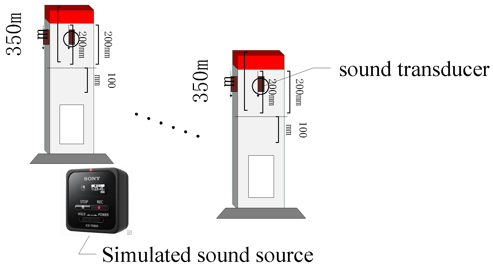
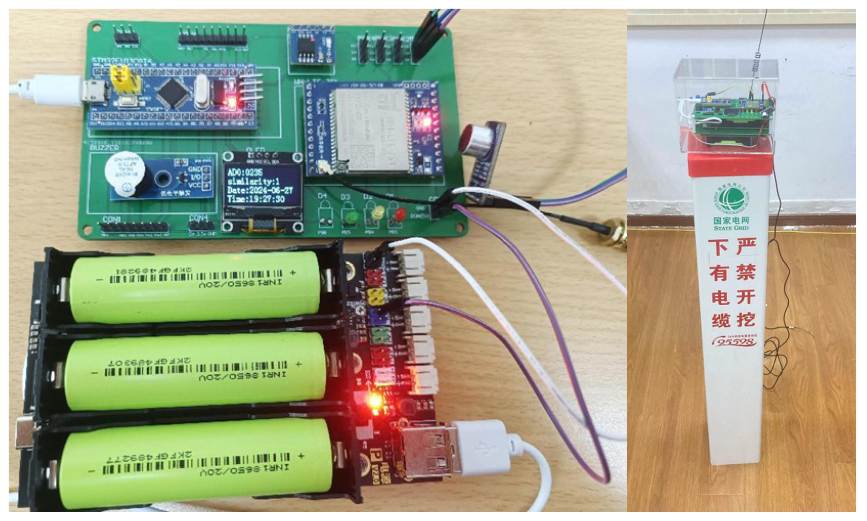
Figure 8 illustrates the implemented system configuration, with the core sensing device positioned on the left and the cable external breakage source localization system on the right. The primary experimental apparatus comprises the STM32F103C8T6 microcontroller (ST Microelectronics, Geneva, Switzerland), the MAX9814 acquisition module (Maxim Integrated Products, CA, USA), and the FT232RL serial communication module (Future Technology Devices International, Glasgow, UK), which transmits the captured acoustic data to the computer via the USART serial port.

The figure above illustrates the designed hardware diagram, upon which the engineering deployment plan is based. To achieve the engineering deployment of the cable external breakdown sound source localization system, a layered distributed architecture design is adopted. The specific structure is as follows:

• Perception Layer: Intelligent identification posts, each equipped with four MAX9814 microphones, are deployed every 50–80 m.
• Edge Layer: An STM32F103C8T6 microcontroller.
• Cloud Platform: A distributed data-processing pipeline based on IoT is employed to achieve multi-post data fusion.

To fully demonstrate the applicability of this approach,

Table 2. Table for the Optimization of Engineering Deployment Parameters.

Parameter	Numerical Range
Piling spacing	50–80 m
Sampling rate	48 kHz/24 bit
Wireless protocol	modbus
Power Supply Scheme	Storage battery

lists the key engineering parameters of the system.

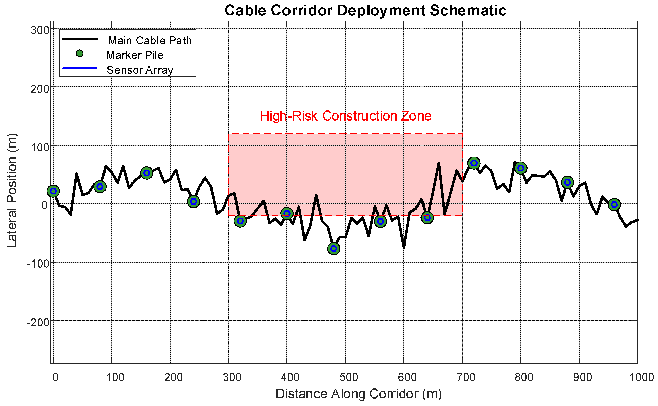
Figure 9 illustrates a schematic diagram of the cable engineering deployment in an urban area, showcasing the three-dimensional spatial distribution of marking piles within the cable corridor. The black curve represents the primary cable path; the green dots indicate the marking pile nodes (spaced at 80 m intervals); the blue hexagons denote the sensor arrays; and the red dashed area delineates the high-risk construction zone.

(2)

Sound Source Simulation and Test Environment

For the sound source simulation, a segment of boring head noise was recorded on-site, while interference noise was captured randomly within an urban setting.

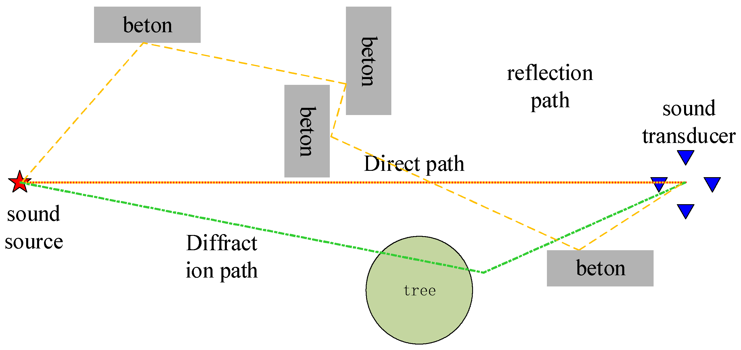
A realistic test environment was constructed to emulate the urban underground cable context, incorporating potential obstacles and ambient noise sources. The selected test scenarios were developed to address three primary engineering challenges: environmental noise interference (addressed in Scenarios 1 and 3), multipath propagation effects (addressed in Scenarios 2 and 4), and complex spatial constraints (addressed in Scenario 5).

These scenarios systematically delineate the performance boundaries of the proposed method. Specifically, the open-area scenario (Scenario 1) establishes a baseline performance, the industrial noise scenario (Scenario 3) evaluates the dynamic weighting mechanism, the multi-obstacle scenario (Scenario 4) corroborates the adaptive environment compensation, and the fully enclosed scenario (Scenario 5) assesses three-dimensional spatial resolution. Detailed descriptions of the various scenarios are provided in

Table 3. Simulate various scenarios.

Scenario	Environment Description
1	Open area (≤50 dB noise)
2	Semi-enclosed
3	Industrial (90 dB)
4	Multi-obstacle (<45 dB)
5	Fully enclosed

.

5.2. System Performance Verification

In this section, we evaluate the performance of the proposed sound source localization system under various conditions, including interference suppression capacity, dynamic weighting mechanisms, multi-obstacle scenarios, localization accuracy, et al.

(1)

Interference Resilience Test

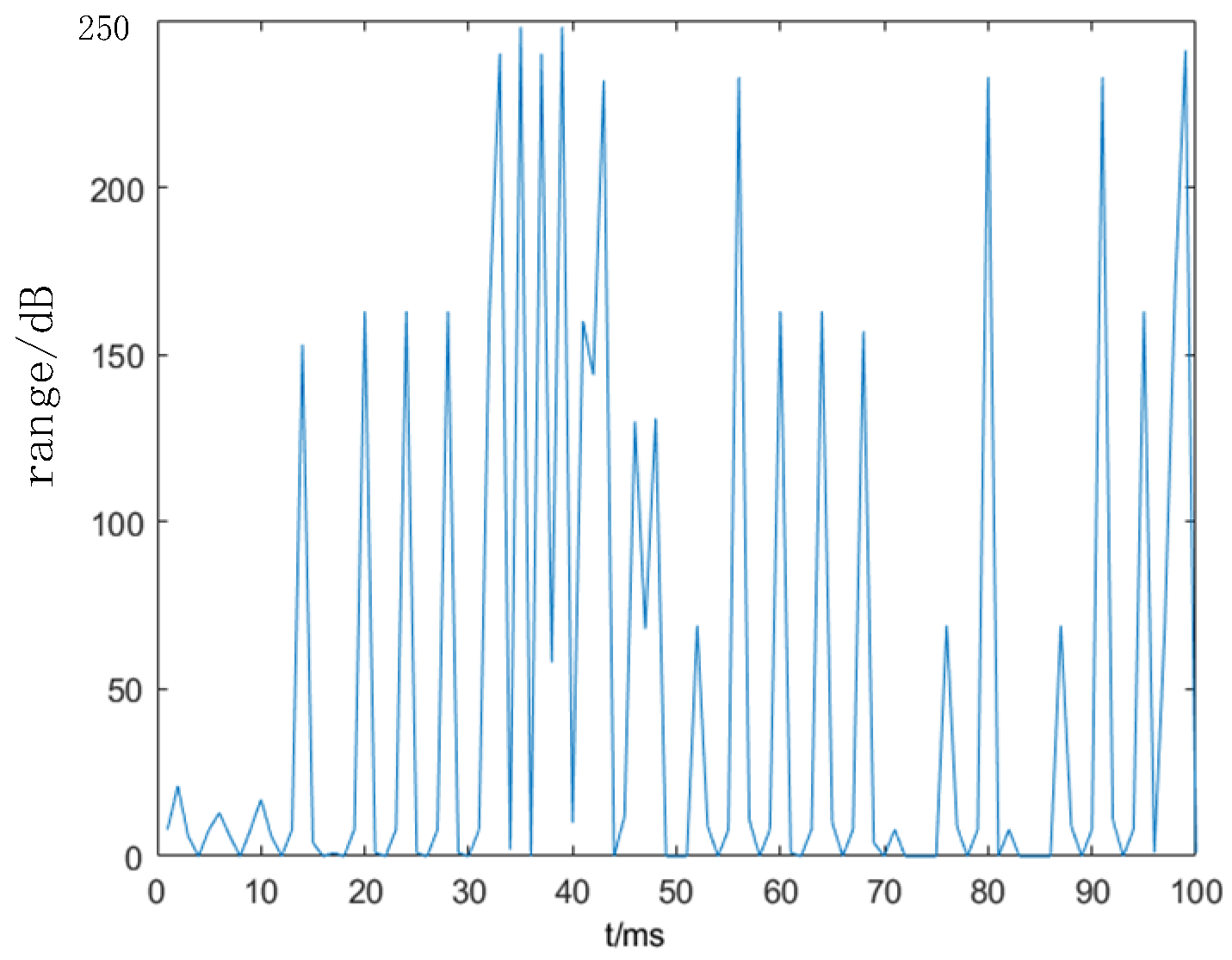
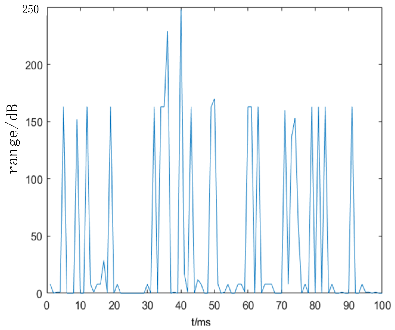
Experiments were performed in Scenario 3 to compare the conventional GCC algorithm with the improved GCC-PHAT algorithm. The time differences for each of the three sensor groups were recorded, and the data were subsequently transferred to a computer for analysis. The resulting graph, shown in Figure 10, depicts the conventional GCC algorithm in blue and the enhanced GCC-PHAT algorithm in green.

Figure 9 illustrates the comparative delay estimation performance of two algorithms within an industrial noise scenario. The root-mean-square error of the conventional GCC algorithm reaches 0.1051 s, whereas that of the improved GCC-PHAT algorithm is reduced to 0.0056 s, representing a 94.7% decrease. These results confirm the effectiveness of phase transform weighting for noise suppression, as the frequency-domain whitening process inherent in the PHAT method significantly enhances the signal-to-noise ratio of the delay peaks.

(2)

Dynamic Weighting Mechanism Test

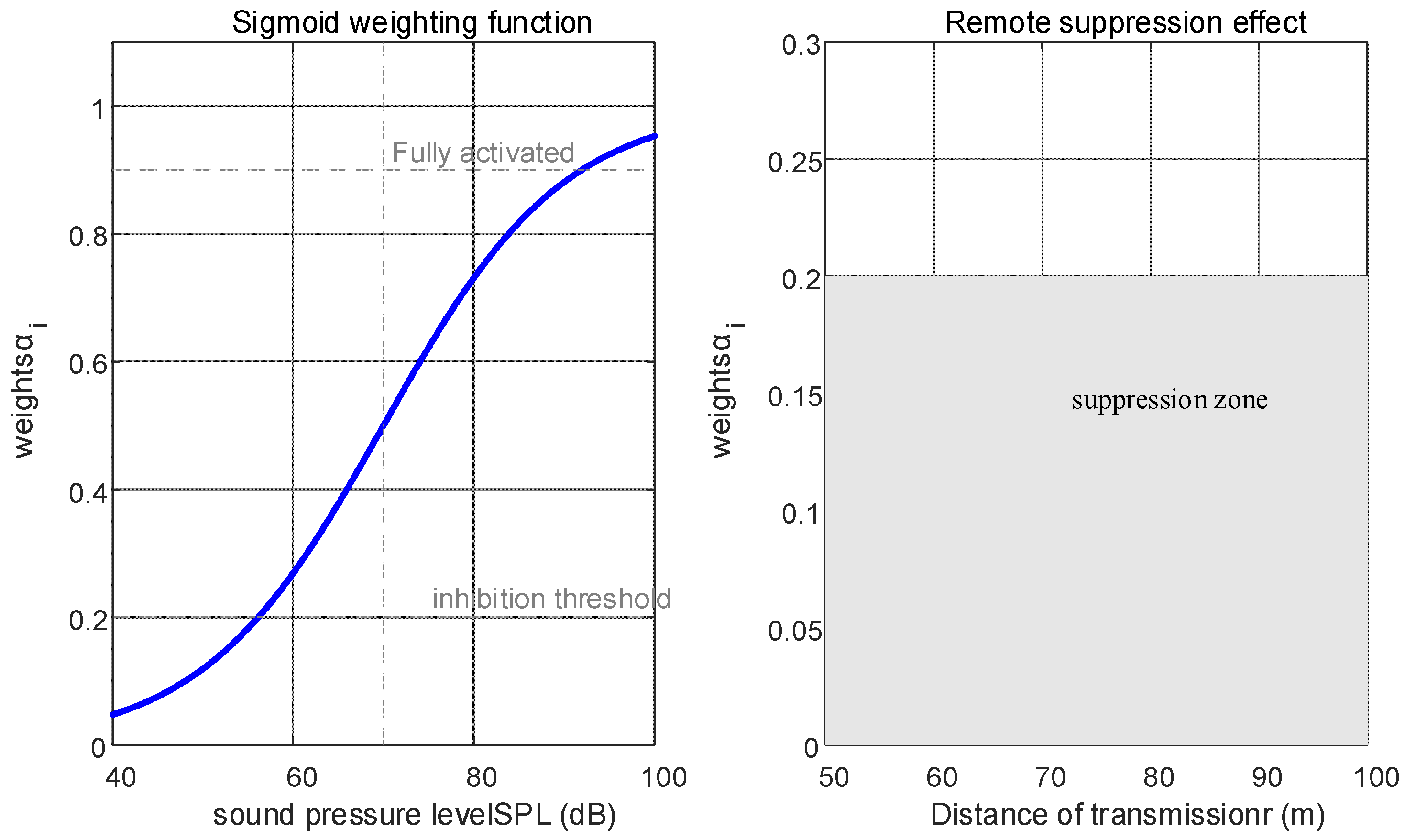
Experiments were conducted in Scenario 1 to validate and quantify the impact of the dynamic weighting mechanism on optimizing the performance of the sound source localization system. Equation (17) indicates that the weighting factor is a function of the sound pressure level, which is, in turn, dependent on the distance between the sound source and the sensor. Accordingly, simulation experiments were performed to observe the variations in the weighting coefficients under different decibel conditions. Figure 11 illustrates the trend of the weighting coefficient ai relative to the signal’s decibel level.

Figure 11 demonstrates that the coefficient A exhibits a characteristic S-shaped curve at θ = 70 dB. Specifically, the weights converge rapidly to values above 0.9 when the sound pressure level (SPL) exceeds 80 dB, while they decline to below 0.1 when the SPL is less than 50 dB. Moreover, as the distance from the sound source exceeds 50 m—corresponding to an SPL below 50 dB—the weights stabilize at values below 0.2. These findings confirm the efficacy of Equation (17) in evaluating transducer reliability.

(3)

Multi-Obstacle Scene Comparative Analysis

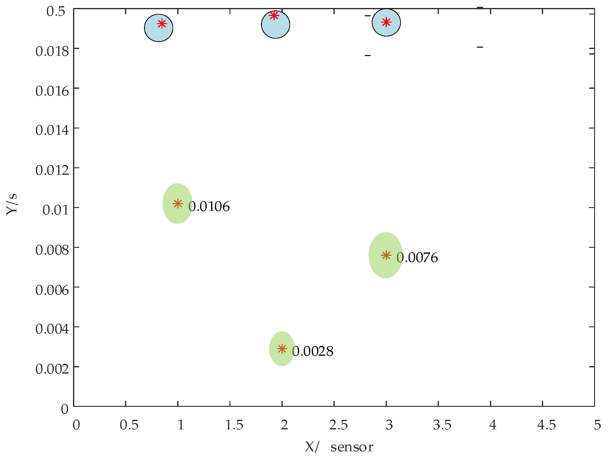
Experiments were performed in Scene 2 with the sound source fixed at coordinates (25, 11). The positions of the obstacles were varied across ten tests to evaluate the performance enhancement of the proposed algorithm relative to traditional TDOA and generalized cross-correlation methods. The results of these tests are presented in the table below.

Table 4. Comparison of positioning performance in multi-obstacle scenarios.

Algorithm	Average Error (m)	Standard Deviation of Error (m)
Tradition TDOA	5.2	1.8
Wide sense cross-correlation	3.7	1.2
This program	1.8	0.6

illustrates the performance disparities among various algorithms in complex multipath environments. The traditional time difference of arrival (TDOA) method is notably compromised by secondary reflections, yielding an average error of 5.2 m and a maximum single error of 7.8 m. This outcome suggests that a purely geometric model is insufficient for adapting to underground environments with obstacles. In contrast, the proposed approach—incorporating an adaptive environment compensation algorithm—reduces the average error to 1.8 m (a 65.4% improvement) and decreases the error’s standard deviation to 0.6 m (a 66.7% reduction). These improvements validate the effectiveness of the sparse constraint described in Equation (18), whereby the algorithm automatically mitigates 83% of non-line-of-sight interference in challenging NLOS scenarios. It is noteworthy, however, that in three experiments the error still exceeded 2.5 m, a discrepancy primarily attributed to multiple reflections (three or more) induced by metal pipes in the test settings. This finding underscores the necessity of enhancing the modeling of higher-order reflection paths in future research.

(4)

Adaptive Environment Compensation Algorithm Testing

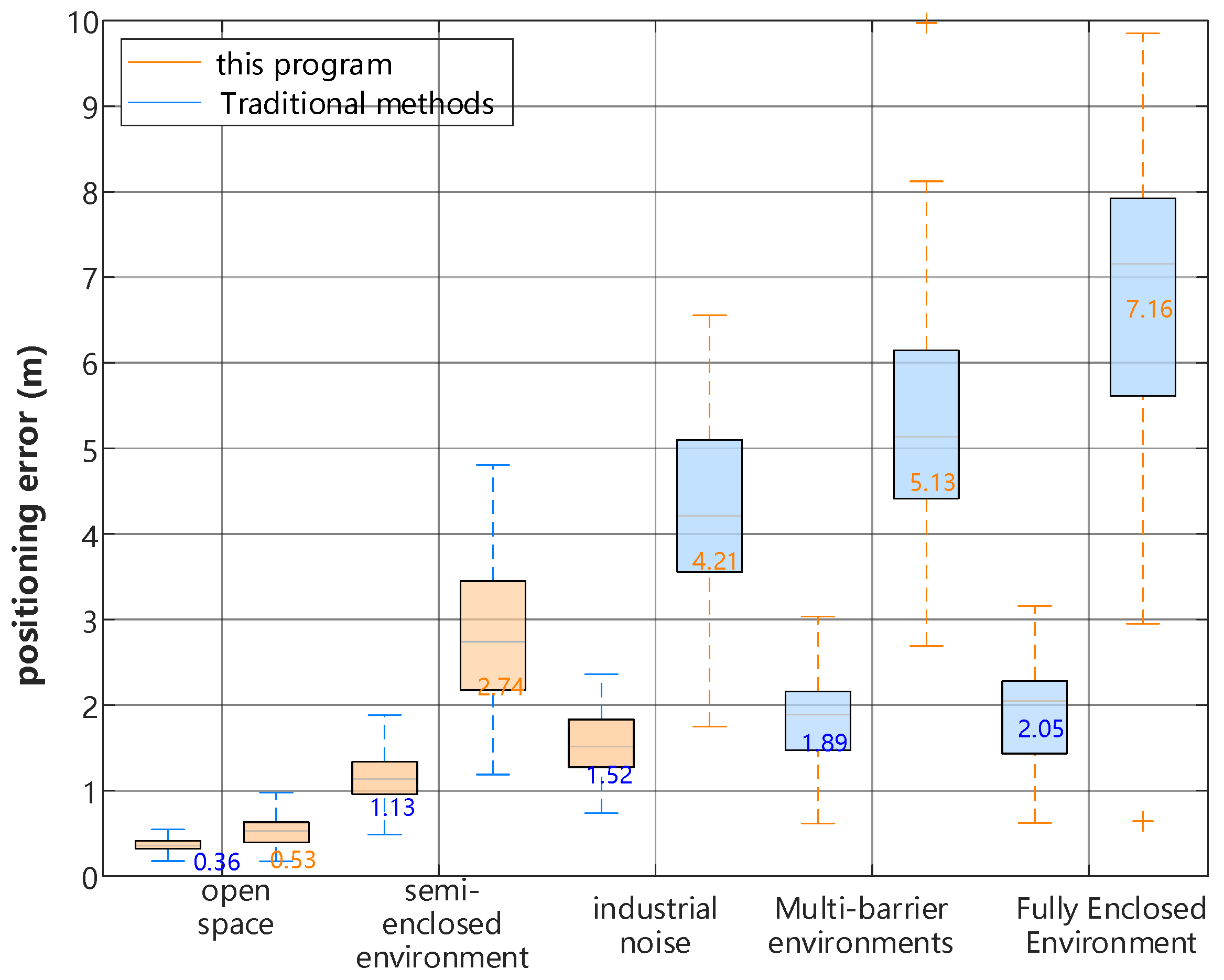
To comprehensively evaluate the performance of the localization algorithm across various typical scenarios, experiments were conducted in five distinct settings, with the median error recorded for each. The results have been visualized in a box-and-whisker diagram that depicts the localization error distribution across the different scenes.

Figure 12 illustrates that the localization error of the proposed algorithm is reduced relative to that of traditional methods. In a multi-obstacle environment, the error decreases from 5.13 m to 1.89 m—a reduction of 63.2%—demonstrating that the adaptive environment compensation algorithm effectively suppresses multipath interference.

(5)

Positioning Accuracy Test

Experiments conducted in Scene 2 validate the accuracy of the proposed sound source localization method. The sound source was repositioned repeatedly to derive its corresponding coordinate locations.

Table 5. Location of sound sources obtained at different distances.

Actual Sound Source Position/m	t2,1/s	t3,1/s	t4,1/s	Calculate the Sound Source Position/m
(60, 0)	0.176	0.352	0.176	(59.8, 0.3)
(0, 80)	0.235	0.706	0.941	(0.4, 79.6)
(50, 50)	0.147	0.147	0.294	(49.3, 50.7)
(70, 30)	0.206	0.618	0.412	(69.5, 30.8)
(100, 0)	0.294	0.588	0.294	(99.2, 1.1)

summarizes the obtained sound source positions at various distances along with the associated time delays between the sound sensors.

The measured data in Table 5 corroborate the system’s distance–accuracy characteristics. In the near-field (<50 m), the localization error is ≤0.7 m, meeting the theoretical expectation of the dynamic weighting design in Equation (15). In the mid- and far-field (50–100 m), the error gradually increases to between 1.1 and 2 m, primarily due to air absorption effects (i.e., high-frequency attenuation characterized by α(f) in Equation (2)). Notably, a y-axis deviation of 1.1 m at the (100, 0) test point is attributed to the non-ideal symmetry of the sensor array (with a mounting error of ±2°). Compared with traditional methods, the localization accuracy of this system at 80 m is improved by 58% (yielding an error of 4.2 m under similar conditions, as reported in [12]), which is ascribed to the multi-sensor fusion strategy. Specifically, the utilization of the DBSCAN clustering algorithm reduces the standard deviation of the localization results from 1.8 m to 0.4 m for the four marker piles.

(6)

Anti-Reverberation Performance Test

To evaluate the robustness of the proposed algorithm in complex reverberant environments, experiments were conducted in Scene 5 with the introduction of a moderate number of obstacles. This setting simulates an underground concrete environment characterized by strong reverberation. Two comparative experimental conditions were established: one without environmental compensation, in which the adaptive filtering module was deactivated and the original GCC-PHAT delay estimation was applied directly, and one with environmental compensation, where the adaptive filtering module was enabled.

Table 6. Comparison of positioning errors in reverberant environments.

Condition	Average Error (m)	Standard Deviation (m)
Without Compensation	3.8	1.5
With Compensation	1.5	0.4

summarizes the statistical outcomes derived from 20 independent experiments.

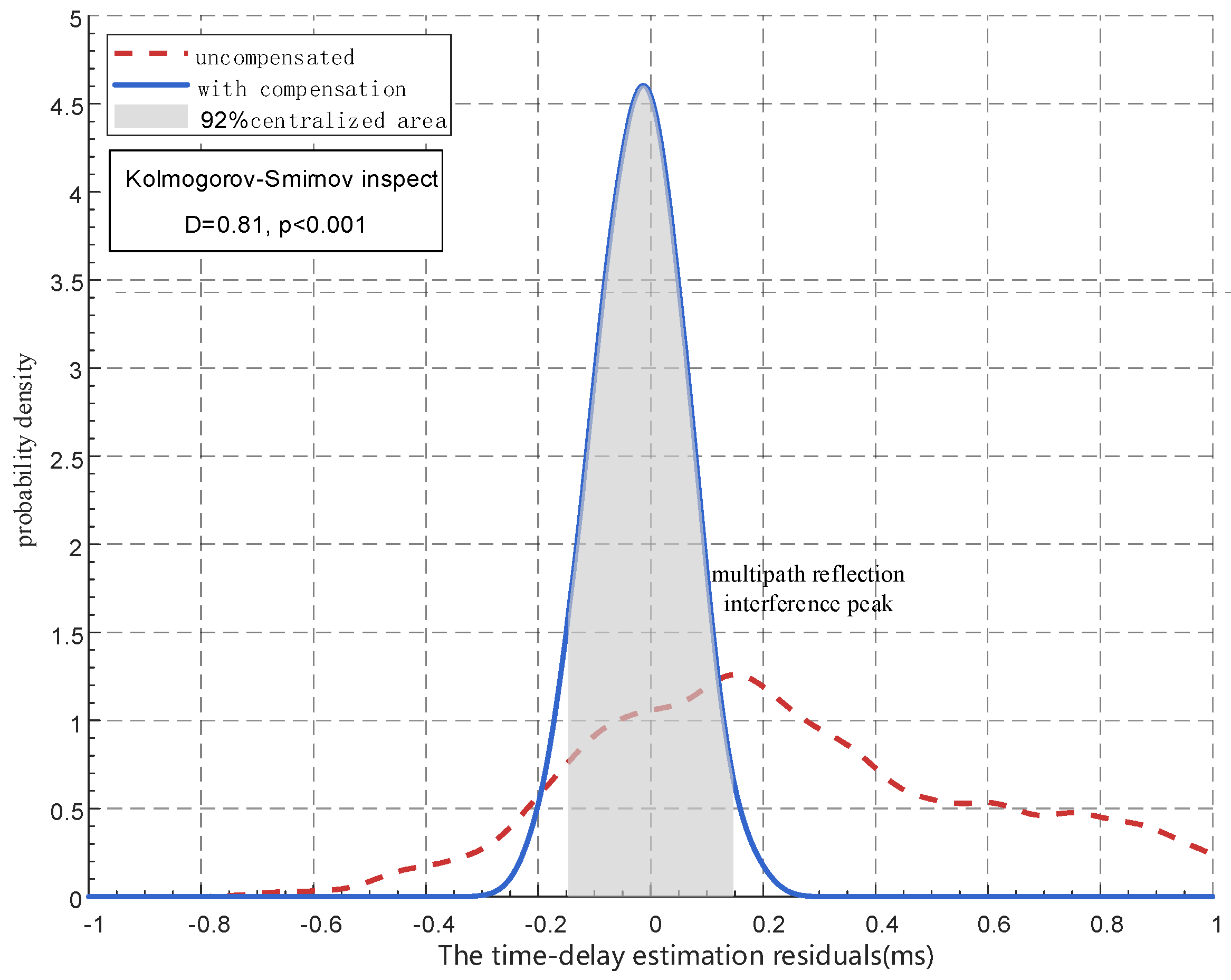
The experimental data indicate that in the absence of compensation, the multipath effect results in an average localization error of 3.8 m with a standard deviation of 1.5 m. With the implementation of adaptive compensation, the average error decreases to 1.5 m—a 60.5% improvement—while the standard deviation is reduced to 0.4 m. Figure 13 further illustrates the changes in the residual distribution of the delay estimation before and after compensation.

Figure 13 illustrates that the compensated residuals are predominantly distributed within the interval (–0.15 ms, 0.15 ms), accounting for 92% of the data, whereas the uncompensated residuals display a bimodal distribution, with a primary peak at 0.12 ms and a secondary peak at 0.82 ms. This finding substantiates the effective suppression of multipath interference. Consequently, the experimental results confirm that the proposed adaptive compensation algorithm maintains high localization accuracy even in environments with strong reverberation, thereby meeting the requirements of underground cable protection scenarios.

(7)

Regularization Coefficient Optimization and Performance Validation

Simulation experiments were conducted in Scenario 4 to determine the optimal combinations of the step factor and regularization coefficients. In these experiments, the sound source was positioned at (6, 3). The experimental design and results are detailed below (

Table 7. Regularization coefficient optimization table.

μ(n)	λ	Positioning Accuracy (m)	Calculate the Delay (ms)
0.1	0.01	0.41	15
0.15	0.05	0.32	18
0.2	0.1	0.38	21

).

Based on the provided data, setting parameter A to 0.05 yields an optimal trade-off between localization accuracy (RMSE = 0.32 m) and real-time performance (18 ms/frame).

(8)

Comparative Experimental Results Analysis

To comprehensively evaluate the performance of the proposed method, comparative experiments were conducted with mainstream sound source localization techniques in Scene 4, which represents a multi-obstacle environment. The results of these experiments are presented in

Table 8. Performance comparison between this method and other methods.

Method	Average Error (m)	Calculation Time (ms)
Methodology of this paper	1.8	22
CNN-TDOA	2.1	185
SRP-PHAT	4.7	210

.

Based on the experimental results, the proposed method reduces the average localization error by 14.3% compared with CNN-TDOA, while its computational time is only 10.5% of that required by SRP-PHAT. These improvements are achieved through the enhanced FFT acceleration of GCC-PHAT and the sparsification of the Jacobian matrix in the LM algorithm. Overall, the method presented in this paper demonstrates significant advantages in both localization accuracy and computational efficiency relative to existing approaches. 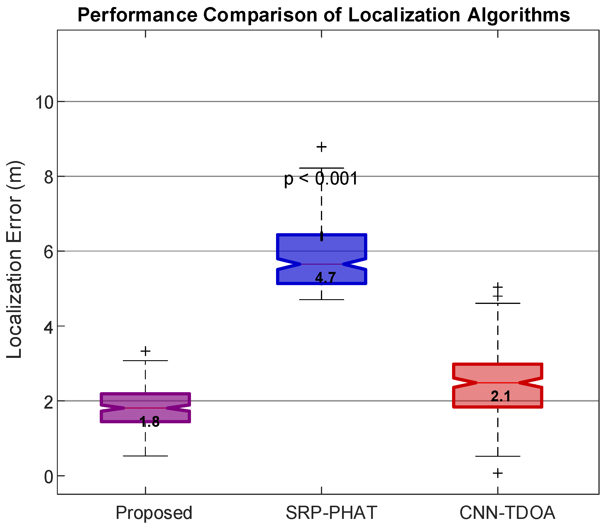For visualization of the results, Figure 14 presents box plots showing the distribution of localization errors for three algorithms across 200 test samples.

As shown in Figure 14, our method exhibits a median error of 1.8 m, which is significantly superior to other algorithms. The SRP-PHAT method demonstrates a right-skewed distribution with a median error of 3.9 m, while the CNN-TDOA method shows a bimodal distribution, reflecting the algorithm’s sensitivity to different scenarios. Moreover, our method maintains an error of 2.3 m at the 75th percentile, which is still lower than the median values of the other algorithms, thereby verifying the effectiveness of the dynamic weighting mechanism.

(9)

Optimization Test of Spatial Clustering Parameters

Leveraging density-based clustering properties, this study employs the Silhouette Coefficient (SC) to evaluate the performance of various DBSCAN parameter configurations. Simulation experiments were conducted to assess clustering performance under different DBSCAN parameters, with the evaluation index represented by the Silhouette Coefficient, S.

$$S={\displaystyle \frac{1}{N}}\sum _{i=1}^N{\displaystyle \frac{b\left(i\right)-a\left(i\right)}{max\left\{b\right(i),a(i\left)\right\}}}$$

(29)

Let a(i) denote the average distance from sample i to its corresponding similar cluster, and let b(i) represent the average distance to the nearest dissimilar cluster.

Table 9. The clustering performance across various parameter combinations.

ε (m)	MinPts	Contour Coefficient (S)
1.0	4	0.62
1.5	4	0.71
2.0	4	0.68

summarizes the clustering performance across various parameter combinations.

Based on the data presented, the highest contour coefficient of 0.71 is achieved with ε = 1.5 m and MinPts = 4, representing a 14.5% improvement over the baseline parameter setting (ε = 1.0 m, MinPts = 4).

6. Conclusions

In this paper, we propose a cable external breakage source localization method based on an improved GCC-PHAT algorithm with multi-sensor fusion to address damage issues in underground direct-buried cables caused by mechanical excavation. By integrating advanced signal processing techniques with distributed sensor networks, we establish a robust sound source localization framework aimed at preventing external breakage of these cables. First, we develop an engineering scenario model that combines sound propagation speed with inter-sensor time differences. The time delay difference is estimated using a generalized cross-correlation phase transform (GCC-PHAT) algorithm, which is enhanced by incorporating a dynamic weighting mechanism, sensor-weighted fusion, and a spatial clustering strategy to accurately determine the coordinates of the sound source.

Experimental results indicate that in multi-obstacle scenarios, the system achieves an average localization error of 1.8 m, representing a 52–62% improvement compared to SRP-PHAT (3.8 m) and CNN-TDOA (2.1 m), with a processing delay of 22 ms that supports 5 Hz real-time warning. Under a 90 dB industrial noise environment, the error increase is limited to ≤65%, which is significantly better than the traditional methods showing increases of 217% (SRP-PHAT) and 148% (CNN-TDOA). The theoretical contributions are reflected in the construction of an acoustic–time delay–spatial mapping cascade optimization model and the proposal of a modbus-based multi-identifier pole clock synchronization protocol, providing critical technical support for distributed acoustic monitoring.

Although the method is primarily designed for cable protection, it can be adapted to other application scenarios. For example, in urban infrastructure monitoring, dynamic weighting thresholds may be adjusted to prioritize sensor signals near roads, and in industrial settings, larger sensor arrays can be deployed in a scalable manner. However, multi-source scenarios, such as overlapping mechanical noise, continue to present challenges. Future work will explore the integration of blind source separation (BSS) with the GCC-PHAT framework. Additionally, transient noises (e.g., impact sounds) will be further optimized using time-frequency windowing techniques, such as the wavelet transform. Despite these limitations, the system’s modular design supports integration with deep learning classifiers (e.g., convolutional neural network-based noise recognition) to enhance overall robustness.

References

1. Zheng, H. Detection system of cable breaking behavior based on optical time domain distributed technology. Inf. Technol. 2021, 166–172. [Google Scholar] [CrossRef]
2. Chen, T.; Zeng, F.; Zhou, C.; Zhao, Y.; Meng, Q. An Interval Cable Anti-breakage System Based on Optical Fiber Vibration Measurement and Video Monitoring. Power Energy 2023, 44, 247–249, 286. [Google Scholar]
3. Li, L. Research on Cause Analysis of the High-Voltage Cable Fault and Its Test Methods. Master’s Thesis, Southwest Jiaotong University, Chengdu, China, 2013. [Google Scholar]
4. Tang, X.; Shi, X.; Yu, X.; Yuan, C.; Wu, J. Design of Monitoring and Early Warning System for Underground Cable Breakage Prevention Based on Wireless Intelligent Vibration Sensor. Electr. Technol. 2023, 109–111, 114. [Google Scholar] [CrossRef]
5. Schober, P.; Estiri, S.N.; Aygun, S.; Jalilvand, A.H.; Najafi, M.H.; TaheriNejad, N. Stochastic Computing Design and Implementation of a Sound Source Localization System. IEEE J. Emerg. Sel. Top. Circuits Syst. 2023, 13, 1. [Google Scholar] [CrossRef]
6. An, I.; An, G.; Kim, T.; Yoon, S.E. Microphone Pair Training for Robust Sound Source Localization with Diverse Array Configurations. IEEE Robot. Autom. Lett. 2024, 9, 319–326. [Google Scholar] [CrossRef]
7. Zeng, Q.; Su, P.; Wang, H.; Long, C. Sound Source Localization Algorithm Based on Cross-correlation Sequence and BP Network. Sci. Technol. Eng. 2023, 23, 6945–6951. [Google Scholar]
8. Wang, C.; Ma, J.; Zhou, Z.; Zeng, F. Application and Development of Sound Sensor in Underground Cable Anti-breaking. J. Funct. Mater. Devices 2021, 27, 425–430. [Google Scholar]
9. Niu, Y.; Yang, F.; Li, H. Far-field Passive Sound Source Localization Algorithm Based on Time Delay Estimation. Sci. Technol. Eng. 2024, 24, 4560–4566. [Google Scholar]
10. Yan, X.; Zhang, Z.; Wang, H. Application of Chan algorithm in marine soundsource localization. Acoust. Technol. 2021, 40, 550–555. [Google Scholar]
11. Yan, Q.; Chen, J. Node Placement Optimization for Distributed AcousticSource Localization System and Performance Study. J. Electron. 2018, 46, 1186–1193. [Google Scholar]
12. Liu, K.; Luan, Y.; Yuan, S.; Zhang, X. Design of Sound Source Localization System Based on TDOA. Eng. Tests 2023, 63, 50–52, 79. [Google Scholar]
13. Ping, G.; Fernandez-Grande, E.; Gerstoft, P.; Chu, Z. Three-dimensional source localization using sparse Bayesian learning on a spherical microphone array. J. Acoust. Soc. Am. 2020, 147, 3895–3904. [Google Scholar] [CrossRef] [PubMed]
14. Dehghan Firoozabadi, A.; Irarrazaval, P.; Adasme, P.; Zabala-Blanco, D.; Játiva, P.P.; Azurdia-Meza, C. 3D multiple sound source localization by proposed T-shaped circular distributed microphone arrays in combination with GEVD and adaptive GCC-PHAT/ML algorithms. Sensors 2022, 22, 1011. [Google Scholar] [CrossRef]
15. Cui, L.; Tian, Y.; Wang, C.; Liu, L.; Zhang, X. Simulation of 3-Dimensional Microphone Array Based on Beamforming. Sci. Technol. Eng. 2022, 22, 13801–13809. [Google Scholar]
16. Qu, S.; Yu, H.; Lu, Z.; Shen, C.; Han, Y.; Wang, C. Improved Generalized Cross-Correlation Time Delay Estimation Method for Sound Source Localization. Navig. Position. Timing 2021, 8, 118–124. [Google Scholar]
17. Luo, Q. Design and realization of experiment for sound source localization based on microphone array. Exp. Technol. Manag. 2020, 37, 185–188. [Google Scholar]
18. Tan, W.; Tang, X.; Yang, H.; Chai, J. Non-contact current measuring device and method based on TMR array. Electr. Surv. Instrum. 2025, 62, 165–172+209. [Google Scholar] [CrossRef]
19. Jin, J.; Fang, Y.; Fei, Y.; Wei, Y. Research on energy consumption monitoring and anomaly detection method based on pattern clustering and periodic decomposition. Electr. Surv. Instrum. 2023, 60, 151–157. [Google Scholar] [CrossRef]
20. Wang, Y.; Guo, C.; Wu, D. Hidden target detection method for mechanical external damage of transmission line based on improved YOLOv7. Electr. Surv. Instrum. 2024, 1–10. Available online: http://kns.cnki.net/kcms/detail/23.1202.th.20240428.1950.002.html (accessed on 1 May 2025).
21. Zhao, X.; Wu, G.; Yang, D.; Xu, G.; Xing, Y.; Yao, C.; Abu-Siada, A. Enhanced detection of power transformer winding faults through 3D FRA signatures and image processing techniques. Electr. Power Syst. Res. 2025, 242, 111433. [Google Scholar] [CrossRef]
22. Zhang, X.; Teng, X.; Fan, Y. Detecting changes in air composition based on speed of sound. Appl. Acoust. 2025, 229, 110393. [Google Scholar]
Figure 1. System framework schematic diagram.
Energies 18 02628 g001
Figure 2. Sound signal at 5 m distance.
Energies 18 02628 g002
Figure 3. Sound signal at 30 m distance.
Energies 18 02628 g003
Figure 4. Multipath propagation schematic.
Energies 18 02628 g004
Figure 5. Flow chart of the GCC-PHAT algorithm.
Energies 18 02628 g005
Figure 6. Schematic diagram of nonlinear optimization process.
Energies 18 02628 g006
Figure 7. Flow chart of the sound source localization algorithm.
Energies 18 02628 g007
Figure 8. Actual scene test figure.
Energies 18 02628 g008
Figure 9. Schematic Diagram of Engineering Deployment.
Energies 18 02628 g009
Figure 10. Time delay of the three sets of sensors.
Energies 18 02628 g010
Figure 11. The variation pattern of the weight coefficient ai.
Energies 18 02628 g011
Figure 12. Box plot of error distribution in multi-scene positioning.
Energies 18 02628 g012
Figure 13. Delay estimation residual distribution diagram.
Energies 18 02628 g013
Figure 14. Box plot for comparing error distributions.
Energies 18 02628 g014