Modelling and Simulation of Pico- and Nano-Grids for Renewable Energy Integration in a Campus Microgrid

Abstract

Research in renewable energy sources and microgrid systems is critical for the evolving power industry. This paper examines the operational behavior of both pico- and nano-grids during transitions between grid-connected and islanded modes. Simulation results demonstrate that both grids effectively balance the power flow, regulate the state of charge (SOC), and stabilize the voltage during dynamic operational changes. Specific scenarios, including grid disconnection, load sharing, and weather-based energy fluctuations, were tested and validated. This paper models both pico-grids and nano-grids at the Singapore Institute of Technology Punggol Campus, incorporating solar PVs, energy storage systems (ESSs), power electronic converters, and both DC and AC loads, along with utility grid connections. The pico-grid includes a battery storage system, a single-phase inverter linked to a single-phase grid, and DC and AC loads. The nano-grid comprises solar PV panels, a boost converter, a battery storage system, a three-phase inverter connected to a three-phase grid, and AC loads. Both the pico-grid and nano-grid are configurable in standalone or grid-connected modes. This configuration flexibility allows for a detailed operational analysis under various conditions. This study conducted subsystem-level modelling before integrating all components into a simulation environment. MATLAB/Simulink version R2024b was utilized to model, simulate, and analyze the power flow in both the pico-grid and nano-grid under different operating conditions.

1. Introduction

The global shift towards a clean energy environment has significantly driven the study of renewable energy sources (RESs). These sources are heralded for their environmental friendliness due to their minimal or zero emissions compared to traditional fossil fuels, which are major contributors to carbon dioxide emissions, greenhouse gases, and overall environmental pollution [1]. As a response to these environmental challenges, there has been a substantial move towards RES-like hydroelectric, biomass, wind, solar, wave, tidal, and geothermal energy, which are continually replenished by nature [2].

The integration of RESs within smart grid technology is a crucial development, bridging the gap between energy demand and supply. Smart grids, equipped with advanced metering systems (AMSs), energy management systems (EMSs), and advanced communication systems, manage the distribution and optimization of renewable energy more effectively than conventional grids. They handle challenges in supply–demand balance, power generation, distribution, and electricity pricing more adeptly [3,4].

This paper aims to investigate the operational characteristics of pico- and nano-grids, particularly their behavior during connection and disconnection from a larger microgrid. By simulating various scenarios, this paper explores how these grids maintain energy balance and support reliable operation under both grid-connected and islanded conditions. This study emphasizes the importance of seamless transitions in ensuring the efficiency and reliability of microgrid systems. The nano-grid, suitable for individual buildings, and the pico-grid, designed for standalone applications within a building, aim to demonstrate how the integration of solar photovoltaic (PV) systems and energy storage can optimize the power flow and enhance grid reliability. The smaller power networks, pico-grids and nano-grids, should be able to function both in an islanded (stand-alone) and a grid-connected mode and should be able to operate steadily in a cluster [5]. In [6], a comprehensive review of the recent developments in nano-grid research, including the control topologies and methods that allow for the nano-grid’s intelligent control, are covered. Significant advances have been made in nano-grid control and energy management, particularly concerning the seamless operation of interconnected systems. Ref. [7] focuses on optimal energy management in microgrids and nano-grids, addressing the challenges posed by uncertainty in renewable energy sources. This is aligned with our study’s focus on grid-connected and islanded modes of operation for pico- and nano-grids. The operation of a basic nano-grid with a rule-based controller and load behavior in response to fluctuating renewable energy source electricity availability is modelled in [8]. The concept and architecture of Open Energy Systems (OESs) for a higher-level control of the components of a standalone nano-grid is introduced in [9]. In [10], the use of an optimal energy management system to mitigate the impact of energy uncertainties in an interconnection between microgrid–nano-grid were studied. The power management of a nano-grid for grid support and deploying power converters to regulate power quality is discussed in [11]. Newer studies specifically addressing nano-grid control are reported in the literature. For example, ref. [12] explores power management and control systems in low-voltage DC nano-grids, which are highly relevant to the load management strategies presented in our study. The hybrid AC/DC control framework proposed by [13] provides valuable insights into managing energy sources in nano-grids. In [14], an adaptive hierarchical control strategy using fuzzy logic is proposed to improve nano-grid energy management, which echoes our control approach. The droop control method for dynamic power sharing in nano-grid clusters by [15] is another example of a control strategy that could be applied to improve our system’s responsiveness and efficiency.

The integration of advanced communication technologies like cloud computing and IoT in smart grids is required to support the use of smart energy management systems (EMSs) to optimize a microgrid’s or nano-grid’s performance [16]. Recent research and development efforts in nano-grids are also focusing on the ability to interconnect nano-grids to trade energy [17,18]. An extensive review of peer-to-peer (P2P) energy trading in smart grids, including mechanisms and challenges, is presented in [19]. These authors emphasize the importance of decentralized frameworks, such as blockchains, for energy trading between nano-grids. A decentralized blockchain mechanism for a demand–response program in nano-grids is proposed in [20]. A predictive optimization-based model for an optimal energy sharing plan between a cluster of nano-grids is proposed in [21]. Peer-to-peer energy trading platforms can encourage the formation of federated power plants within local grids, including nano-grids, which will enable a more resilient power system [22]. Importantly, ref. [23] emphasizes the critical role of sustainable energy systems in addressing global energy challenges, focusing on multidisciplinary approaches to integrate renewable sources effectively. This aligns with the modelling of pico- and nano-grids as sustainable solutions for localized energy management, ensuring efficient operation while reducing CO₂ emissions through renewable integration.

With the establishment of the Singapore Institute of Technology (SIT) in Punggol Digital District, a Multi-Energy Microgrid (MEMG) has been implemented and will be fully operational in late 2024, aiming to achieve zero emissions [24]. Approximately 10,000 m² of solar panels will be installed on rooftops to power the campus, significantly reducing reliance on the main utility grid and advancing the institution’s sustainability goals. This development motivates the need for a testbed to model and analyze the operation of both pico-grids and nano-grids in the campus’s west zone.

This paper aims to model and simulate the pico-grid and nano-grid using MATLAB/Simulink to achieve the following:

• Explore and study the individual subsystems of both the pico-grid and nano-grid.
• Model and integrate relevant components.
• Develop simulation models to analyze the power flow.
• Perform tests to assess operations under realistic scenarios.

The primary contributions of this paper include a detailed study, modelling, and simulation of a pico-grid and nano-grid. This work constructs a comprehensive model of these systems using MATLAB/Simulink to facilitate a power flow analysis under various operating conditions. In what follows, Section 2 discusses the proposed architecture for the pico-grid and nano-grid and their modelling. Section 3 presents the test conditions and simulation results. Section 4 concludes the paper and outlines future areas of work.

2. Systems’ Description and Modelling

2.1. Proposed Architecture of Pico-Grid System

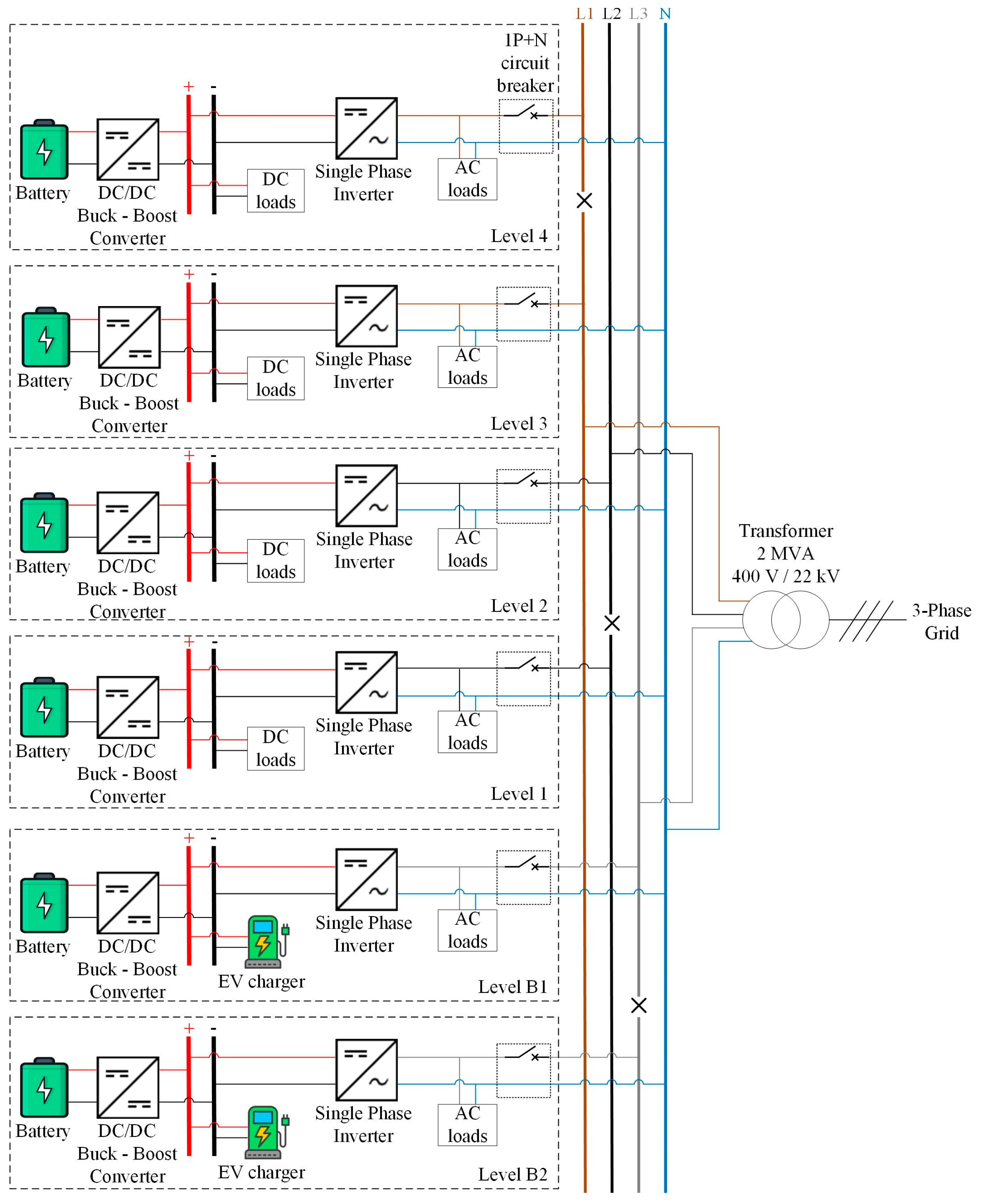
Figure 1 shows the proposed architecture of a pico-grid system to be implemented in various buildings at the SIT Punggol Campus. The building is a six-story structure with two basement car parks and four levels of amenities, including classrooms, lecture theatres, and a server room. Each level is equipped with a standalone pico-grid system to supply power to DC and AC loads. Every two levels are connected via a circuit breaker to one phase of the utility grid, and each level’s pico-grid system includes a 1P+N circuit breaker for the option of an islanded or grid-connected mode. For instance, levels B1 and B2 can be linked and connected to the single-phase grid by closing their respective circuit breakers, allowing load sharing if one level’s demand is higher.

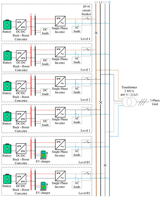
Figure 1. Overview of a pico-grid in a building at SIT Punggol Campus.

The major components of the building are as follows:

• Levels 1 to 4 are designated for classrooms, lecture theatres, and a server room.
• Levels B1 and B2 are used as car parks, each equipped with two electric vehicle chargers.

The pico-grid system includes a battery energy storage system (BESS), a single-phase inverter, DC loads, and AC loads. The primary energy source is the battery, connected to a bidirectional DC/DC buck–boost converter to supply the DC and AC loads. Excess power from the system can be sold back to the grid.

2.1.1. Load Demand of Pico-Grid System

The load demand for each level of a building can be estimated using the Gross Floor Area (GFA). The lighting power demand is calculated according to the Singapore Standard for Energy Efficiency SS530, with the maximum allowable lighting power density (LPD) for different space types outlined in SS530, as shown in Table 1 [25]. The nominal values for receptacle loads for various space types are taken from the Building Construction Authority (BCA) non-residential development Green Mark technical guide, detailed in Table 2 [26].

Table 1. SS530 lighting power density guideline.

Interior Spaces—Type of Usage		LPD (W/m2)
Space-by-space method
Office work and study
Offices, meeting rooms, copy/print rooms, class rooms, lecture theatres, computer rooms, reading areas		12
Laboratories		16
Atrium, halls and retail
Entrance halls, atriums, concourses, lobbies, auditoriums and concert halls		10
Multi-purpose halls, conference halls		16
Retail general lighting and (accent, display, decorative)	Jewelry and crystal	15 (+20)
	Furniture, clothing and accessories, cosmetics, artwork	15 (+10)
	Others, e.g., supermarket, vehicles, sporting goods, hardware and stationery, pharmacy, and undetermined usage during early design	15 (+5)
Food and Relax
Food courts, canteens, hawker centres (including dining area and food preparation)		10
Restaurants, lounges, bars (including dining area and food preparation, accent, display, decorative)		12
Transport and goods
Circulation areas, corridors		7
Stairs, escalators, travelators		6
Lift lobbies		7
Carparks		3
Loading docks		5
Warehouses		7
Storage areas		10

Table 2. Receptacle load values for different spaces.

Receptacle Loads	Nominal Values
Computer-intensive office	22 W/m2
General office areas	16 W/m2
Large conference areas	11 W/m2
Schools (tertiary/IHLs)	8 W/m2
Schools (primary/secondary)	5 W/m2
Server/computer rooms	540 W/m2

The load demand estimation is divided into DC and AC loads. The lighting system, electric vehicle chargers, and server racks are considered DC loads, while receptacle loads such as computers and monitors, which require single-phase power, are considered AC loads. A diversity factor of 50% is assumed for the building.

From Table 3 and Table 4, the estimated lighting system for levels B1 and B2 is 2300 W each, and the receptacle load is 1100 W each. There are two electric vehicle charging stations in the car park areas of B1 and B2, each estimated to require 7 kW/unit, as shown in Table 5.

Table 3. DC load estimation of levels B1 to B2 of SIT Punggol Campus.

BUILDING LIGHTING POWER BUDGET
Description	Areas (m2)	Design Data			SS 530 Requirements
		Design Lighting Power Budget (W/m2)	Lighting Diversity Factor	Total Power Consumption (by Area) (W)	Total Power Consumption (by Area) (W)	Design Lighting Power Budget (W/m2)
B1 to B2 of SIT Punggol Campus
Carpark	700	3	0.5	1050	2100	3
Facilities office	100	12	0.5	600	1200	12
Stairs	100	6	0.5	300	600	6
Lift Lobby A	100	7	0.5	350	700	7
Total	1000			2300	4600

Table 4. AC load estimation of levels B1 to B2 of SIT Punggol Campus.

BUILDING RECEPTACLE LOAD
Description	Areas (m2)	Design Data			SS 530 Requirements
		Design Power Budget (W/m2)	Power Diversity Factor	Total Power Consumption (by Area) (W)	Total Power Consumption (by Area) (W)	Design Power Budget (W/m2)
B1 to B2 of SIT Punggol Campus
Carpark	700	0	0	0	0	0
Facilities office	100	16	0.5	800	1600	16
Stairs	100	1	0.5	50	100	1
Lift Lobby A	100	5	0.5	250	500	5
Total	1000			1100	2200

Table 5. Estimated load demand of electric charging stations for B1 and B2.

ELECTRIC CHARGING STATIONS POWER BUDGET
Levels	Space Type	Quantity	Power (W/unit)	Power Diversity Factor	Total Power Consumption (W)
B1	Electric Charging stations	2	7000	0.5	7000
B2	Electric Charging stations	2	7000	0.5	7000
Total (W)					14,000

From Table 6 and Table 7, the estimated lighting system for levels L1, L2, and L3 is 4900 W each, with a receptacle load of 4150 W each. These levels have higher power consumption due to the presence of amenities such as classrooms and lecture theatres.

Table 6. DC load estimation of levels L1 to L3 of SIT Punggol Campus.

BUILDING LIGHTING POWER BUDGET
Description	Areas (m2)	Design Data			SS 530 Requirements
		Design Lighting Power Budget (W/m2)	Lighting Diversity Factor	Total Power Consumption (by Area) (W)	Total Power Consumption (by Area) (W)	Design Lighting Power Budget (W/m2)
L1 to L3 of SIT Punggol Campus
Classrooms	200	12	0.5	1200	2400	12
Lecture Theatre	200	15	0.5	1500	3000	15
Corridors	300	7	0.5	1050	2100	7
Stairs	100	6	0.5	300	600	6
Lift Lobby A	100	7	0.5	350	700	7
Toilets	100	10	0.5	500	1000	10
Total	1000			4900	9800

Table 7. AC load estimation of levels L1 to L3 of SIT Punggol Campus.

BUILDING RECEPTACLE LOAD
Description	Areas (m2)	Design Data			SS 530 Requirements
		Design Power Budget (W/m2)	Power Diversity Factor	Total Power Consumption (by Area) (W)	Total Power Consumption (by Area) (W)	Design Power Budget (W/m2)
L1 to L3 of SIT Punggol Campus
Classrooms	200	8	0.5	800	1600	8
Lecture Theatre	200	8	0.5	800	1600	8
Corridors	300	5	0.5	750	1500	5
Stairs	100	1	0.5	50	100	1
Lift Lobby A	100	5	0.5	250	500	5
Toilets	100	5	0.5	250	500	5
Total	1000			4150	8300

From Table 8 and Table 9, the estimated lighting system for level L4 is 4350 W, with a receptacle load of 4150 W. Level 4 includes an office area and a server room, which houses four server racks, each estimated at 5 kW/unit, as shown in Table 10.

Table 8. DC load estimation of Level L4 of SIT Punggol Campus.

BUILDING LIGHTING POWER BUDGET
Description	Areas (m2)	Design Data			SS 530 Requirements
		Design Lighting Power Budget (W/m2)	Lighting Diversity Factor	Total Power Consumption (by Area) (W)	Total Power Consumption (by Area) (W)	Design Lighting Power Budget (W/m2)
L4 of SIT Punggol Campus
Server rooms	100	13	0.5	650	1300	13
Offices	300	10	0.5	1500	3000	10
Corridors	300	7	0.5	1050	2100	7
Stairs	100	6	0.5	300	600	6
Lift Lobby A	100	7	0.5	350	700	7
Toilets	100	10	0.5	500	1000	10
Total	1000			4350	8700

Table 9. AC load estimation of level L4 of SIT Punggol Campus.

BUILDING RECEPTACLE LOAD
Description	Areas (m2)	Design Data			SS 530 Requirements
		Design Lighting Power Budget (W/m2)	Lighting Diversity Factor	Total Power Consumption (by Area) (W)	Total Power Consumption (by Area) (W)	Design Lighting Power Budget (W/m2)
L4 of SIT Punggol Campus
Server rooms	100	0	0	0	0	0
Offices	300	16	0.5	2400	4800	16
Corridors	300	5	0.5	750	1500	5
Stairs	100	1	0.5	50	100	1
Lift Lobby A	100	5	0.5	250	500	5
Toilets	100	5	0.5	250	500	5
Total	1000			3700	7400

Table 10. Estimated load demand of server room.

SERVER ROOM POWER BUDGET
Levels	Space Type	Quantity	Power (W/unit)	Power Diversity Factor	Total Power Consumption (W)
L4	Server Racks	4	5000	0.5	10,000
Total (W)					10,000

2.1.2. Modelling of Battery Energy Storage System

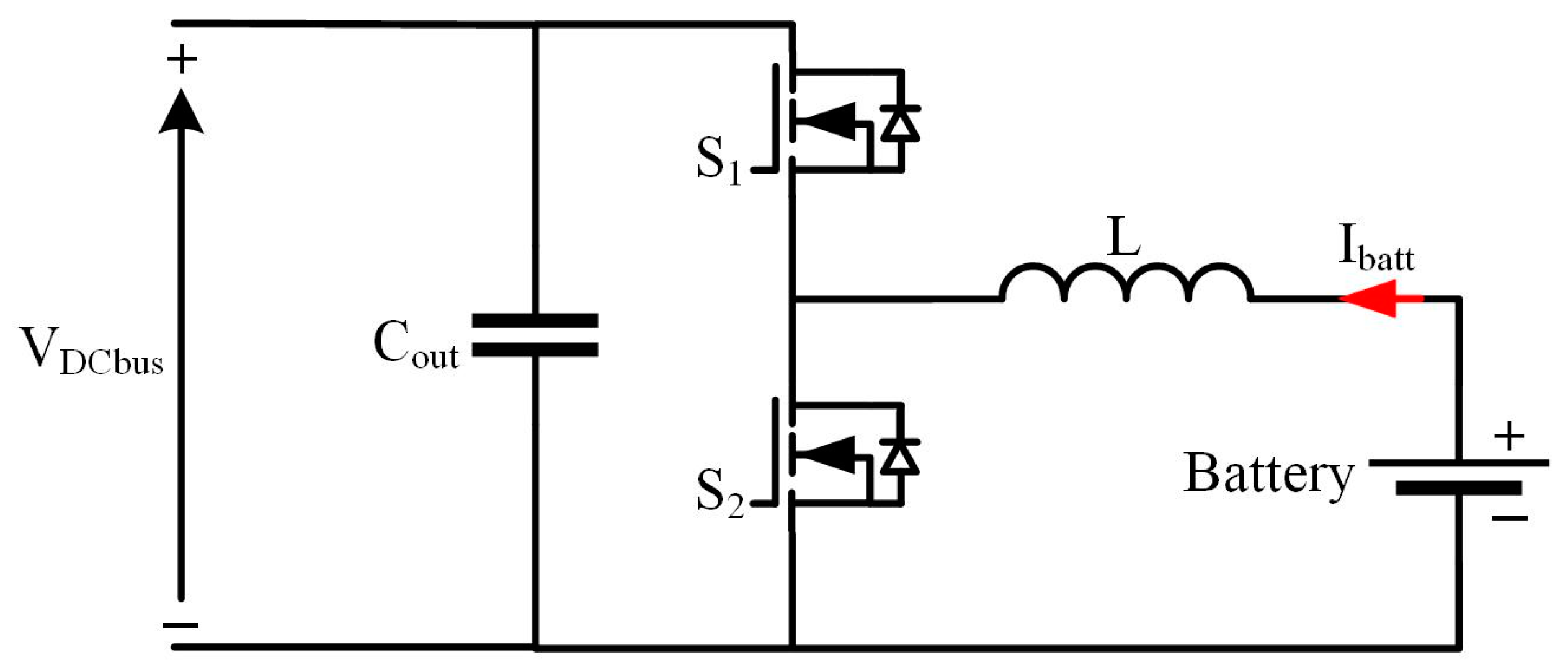
Figure 2 shows the schematic of the BESS using a bidirectional DC/DC converter [27,28]. The topology includes a half-bridge power module, an output capacitor, and an inductor connected to a battery. This system can operate in either boost mode for discharging or buck mode for charging, depending on control inputs. Figure 3 shows the control scheme, utilizing a Proportional Integral (PI) controller and Pulse Width Modulation (PWM) for precise control over the battery output. The simplicity, ease of implementation, and reliability of PI control make it an appropriate choice for real-time energy balancing in pico- and nano-grids, particularly where the system response needs to be fast and stable under dynamic load conditions. PI controllers have a long history of applications in actual microgrid control due to their straightforward tuning process and predictable behavior in handling system transients.

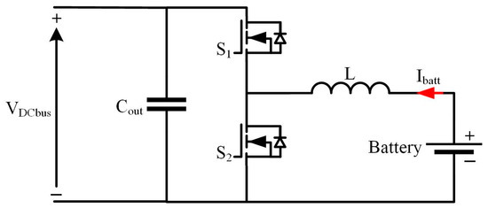
Figure 2. Proposed topology used in BESS.

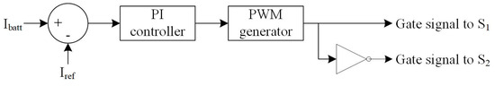
Figure 3. Proposed control algorithm used to control BESS.

To calculate the power stage in boost and buck modes, three key parameters are needed: input voltage, nominal output voltage, and maximum output current. The first step is to determine the duty cycle (D), which is essential for calculating the maximum switching current. The minimum input voltage is used in Equation (1) to determine this maximum switching current.

$$\mathrm{D}=1-{\displaystyle \frac{{\mathrm{V}}_{\mathrm{in}\left(\min \right)}}{{\mathrm{V}}_{\mathrm{out}}}}$$

(1)

The inductor is a key component of the topology, as its value determines the maximum output current. Before calculating the inductor value, the inductor ripple current must be determined, typically estimated at 20% to 40% of the maximum output current ripple. Equations (2) and (3) are used to calculate the inductor ripple current. Once this value is obtained, the estimated inductor value can be determined using Equation (4).

$${\mathrm{I}}_{\mathrm{out}\left(\max \right)}={\displaystyle \frac{{\mathrm{P}}_{\mathrm{out}}}{{\mathrm{V}}_{\mathrm{out}}}}$$

(2)

$$\Delta {\mathrm{I}}_{\mathrm{L}}=\left(0.2\mathrm{to}0.4\right)\times {\mathrm{I}}_{\mathrm{out}\left(\max \right)}\times {\displaystyle \frac{{\mathrm{V}}_{\mathrm{out}}}{{\mathrm{V}}_{\mathrm{in}}}}$$

(3)

$$\mathrm{L}={\displaystyle \frac{{\mathrm{V}}_{\mathrm{in}}\times \left({\mathrm{V}}_{\mathrm{out}}-{\mathrm{V}}_{\mathrm{in}}\right)}{\Delta {\mathrm{I}}_{\mathrm{L}}\times {\mathrm{F}}_{\mathrm{s}}\times {\mathrm{V}}_{\mathrm{out}}}}$$

(4)

The output capacitor value is determined by calculating the ripple voltage, typically estimated at 1% to 5% of the output voltage. Equation (5) is used to calculate the ripple voltage. With this value, the minimum output capacitor value can be found using Equation (6).

$$\Delta {\mathrm{V}}_{\mathrm{out}}=\left(1\%\mathrm{to}5\%\right)\times {\mathrm{I}}_{\mathrm{out}\left(\max \right)}\times {\mathrm{V}}_{\mathrm{out}}$$

(5)

$${\mathrm{C}}_{\mathrm{out}\left(\min \right)}={\displaystyle \frac{{\mathrm{I}}_{\mathrm{out}\left(\max \right)}\times \mathrm{D}}{{\mathrm{F}}_{\mathrm{s}}\times \Delta {\mathrm{V}}_{\mathrm{out}}}}$$

(6)

For the buck mode operation of the bidirectional converter, the same calculation sequence is used, following the buck converter formulas. The ripple current and voltage are calculated similarly to the boost mode. The duty cycle is calculated using Equation (7), the inductor value using Equation (8), and the minimum output capacitor using Equation (9).

$$\mathrm{D}={\displaystyle \frac{{\mathrm{V}}_{\mathrm{out}}}{{\mathrm{V}}_{\mathrm{in}\left(\max \right)}}}$$

(7)

$$\mathrm{L}={\displaystyle \frac{{\mathrm{V}}_{\mathrm{out}}\times \left({\mathrm{V}}_{\mathrm{in}}-{\mathrm{V}}_{\mathrm{out}}\right)}{\Delta {\mathrm{I}}_{\mathrm{L}}\times {\mathrm{F}}_{\mathrm{s}}\times {\mathrm{V}}_{\mathrm{in}}}}$$

(8)

$${\mathrm{C}}_{\mathrm{out}\left(\min \right)}={\displaystyle \frac{\Delta {\mathrm{I}}_{\mathrm{L}}}{8\times {\mathrm{F}}_{\mathrm{s}}\times \Delta {\mathrm{V}}_{\mathrm{out}}}}$$

(9)

2.1.3. Modelling of Single-Phase Inverter

Figure 4 shows the schematic of a single-phase inverter [27]. This inverter uses two half-bridge modules connected to an inductor, output capacitor, and an AC source to mimic an AC grid. The switch pairs S1 and S4 and S2 and S3 operate together. The switching states of the inverter is shown in Table 11.

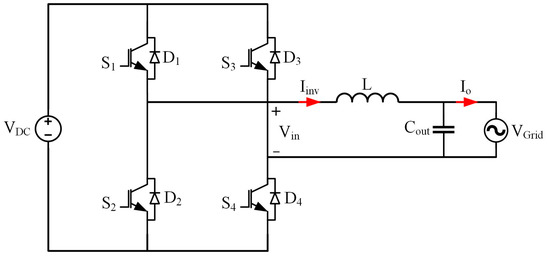
Figure 4. Proposed topology used in single-phase inverter.

Table 11. Switching states of the single-phase inverter.

Cycle	S1	S2	S3	S4	Voltage at Bridge Output	State
Positive half cycle	ON	OFF	OFF	ON	VDC	1
	OFF	ON	OFF	ON	0	2
Negative half cycle	OFF	ON	ON	OFF	−VDC	3
	ON	OFF	ON	OFF	0	4

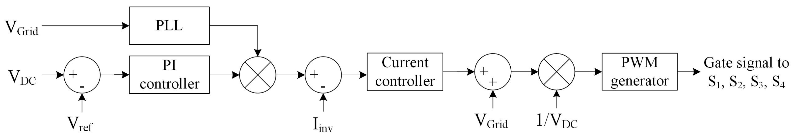
Since the single-phase inverter is connected to the BESS, it is essential to maintain the voltage at the DC busbar. Figure 5 shows the control scheme used for this inverter. To control the gating signals of S1, S2, S3, and S4, the actual DC bus voltage is compared to a reference value to generate an error signal, which is fed into a PI controller. The output of the Phase Lock Loop (PLL) is multiplied with the PI controller’s output, and the inverter current I_inv is subtracted from this result. This error is then processed by a Proportional Resonant (PR) current controller, and the output is added to the voltage set by V_grid. Finally, this output is multiplied by $1/{\mathrm{V}}_{\mathrm{DC}}$ to determine the duty cycle, which is used by a PWM generator to generate the gating signals for the switches.

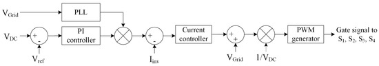
Figure 5. Proposed control algorithm used to control single-phase inverter.

To determine the power stage of a single-phase inverter, three critical parameters must be considered: input voltage, nominal output voltage, and maximum output current. A key aspect of this topology is the filter design before connecting to the grid. First, the RMS current value for the desired grid voltage must be determined, followed by the system’s peak current, as shown in Equations (10) and (11), respectively. Using the peak current, the inductor ripple current—typically between 20% and 40% of the peak current—can be calculated using Equation (12). Finally, with the calculated inductor ripple current, the inductor value is determined using Equation (13).

$${\mathrm{I}}_{\mathrm{out}\left(\mathrm{rms}\right)}={\displaystyle \frac{{\mathrm{P}}_{\mathrm{out}}}{{\mathrm{V}}_{\mathrm{out}\left(\mathrm{rms}\right)}}}$$

(10)

$${\mathrm{I}}_{\mathrm{peak}}={\mathrm{I}}_{\mathrm{out}\left(\mathrm{rms}\right)}\times \sqrt{2}$$

(11)

$$\Delta {\mathrm{I}}_{\mathrm{peak}}=\left(20\%\mathrm{to}40\%\right)\times {\mathrm{I}}_{\mathrm{peak}}$$

(12)

$$\mathrm{L}={\displaystyle \frac{{\mathrm{V}}_{\mathrm{in}}}{4\times {\mathrm{F}}_{\mathrm{s}}\times \Delta {\mathrm{I}}_{\mathrm{peak}}}}$$

(13)

The value of the filter capacitor is estimated using the cutoff frequency of an LC filter. For effective attenuation of the switching frequency, the cutoff frequency is set at one-tenth or less of the switching frequency. By comparing Equations (14) and (15), the final equation for capacitance is derived and shown in Equation (16).

$${\mathrm{F}}_{\mathrm{c}}={\displaystyle \frac{1}{2\mathsf{\pi }\sqrt{\mathrm{LC}}}}$$

(14)

$${\mathrm{F}}_{\mathrm{c}}\le {\displaystyle \frac{{\mathrm{F}}_{\mathrm{sw}}}{10}}$$

(15)

$$\mathrm{C}={\displaystyle \frac{10}{2{\mathsf{\pi }\mathrm{F}}_{\mathrm{s}}}}\times {\displaystyle \frac{1}{\mathrm{L}}}$$

(16)

2.2. Proposed Architecture of Nano-Grid System

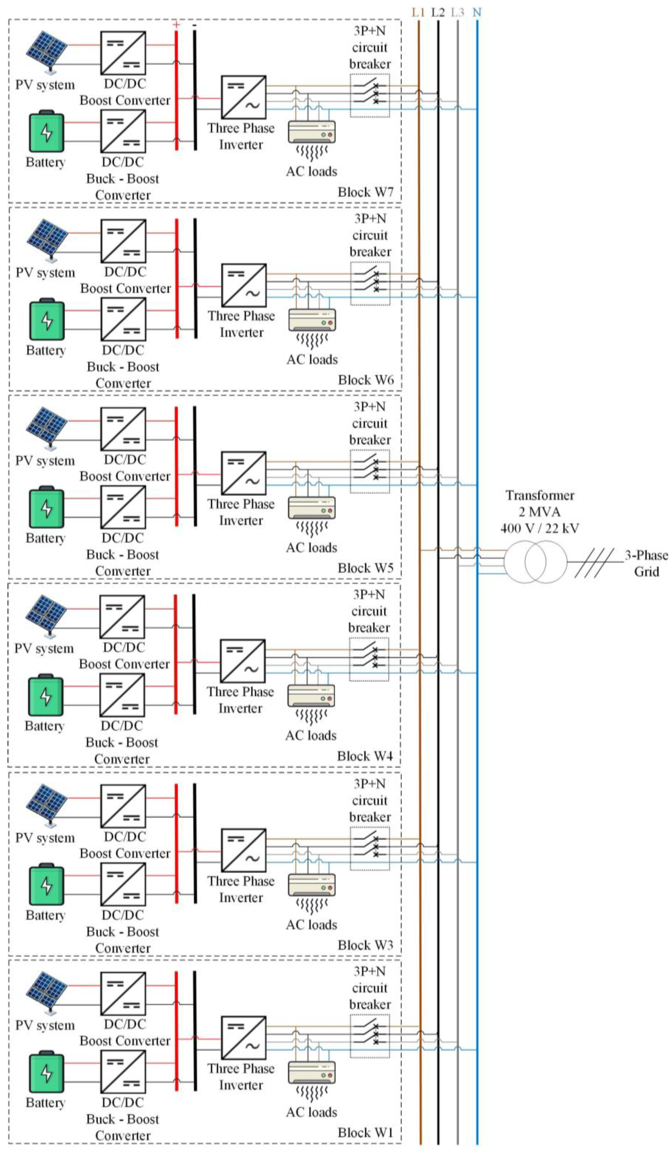
Figure 6 shows the proposed nano-grid system architecture designed to power an entire building at the SIT Punggol Campus. Each nano-grid in the building includes a 3P+1N circuit breaker prior to connecting to the grid. These circuit breakers are normally closed; thus, each building’s nano-grid remains connected to the utility grid. This setup enables the nano-grid to function in either islanded or grid-connected modes. In grid-connected mode, it supports load sharing with other nano-grids, while in islanded mode, it operates independently.

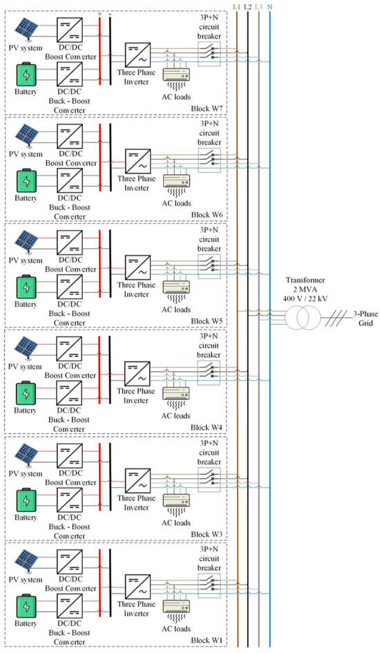
Figure 6. Overview of nano-grid system of a building at SIT Punggol Campus.

The nano-grid system consists of a solar PV array, a BESS, a three-phase inverter, and AC loads. The solar PV and battery storage serve as the main energy sources. On the DC side, the solar PV connects to a boost converter regulated by an MPPT controller, with its output feeding into the DC busbar. The battery connects through a bidirectional DC/DC buck–boost converter, also feeding into the DC busbar. A three-phase inverter links to the DC busbar, with its output directed to AC loads and the utility grid.

2.2.1. Load Demand of a Nano-Grid System

Table 12 shows the load demand for the nano-grid system. For this study, only AC loads are included, focusing on the centralized cooling system for the building. Air conditioning is required for four levels, with an estimated cooling power of 20 W/m² and a diversity factor of 50%. The total power consumption was calculated to be 40 kW. This value will be used in the simulation model in Section 3.

Table 12. Load demand estimation for centralized cooling.

BUILDING COOLING POWER BUDGET
Levels	Space Type	Areas (m2)	No of Floors	Cooling Power (W/m2)	Cooling Power Diversity Factor	Total Power Consumption (by Area) (W)
L1 to L4	School building	1000	4	20	0.5	40,000
Total (W)						40,000

2.2.2. Modelling of Solar PV Boost Converter

Figure 7 shows the schematic of a boost converter integrated with a solar PV system [29,30]. The proposed design for the solar PV boost converter includes a MOSFET, a diode, an output capacitor, and an inductor connected to a solar array module. The converter operates in Continuous Conduction Mode (CCM). When MOSFET S1 is activated, the inductor stores energy. When S1 is deactivated, the inductor’s current decreases, causing it to act as a voltage source in series with the input voltage, thus regulating the output voltage. The boost converter is modelled using Equations (1) to (6).

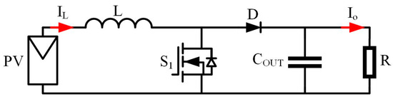
Figure 7. Proposed topology used in solar PV boost converter.

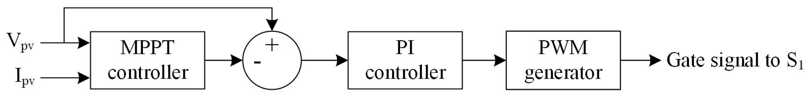
Figure 8 shows the control scheme for the solar PV boost converter. A PI controller is employed to generate the duty cycle, which is then fed into a PWM generator to produce the gating signal for S1. There are other alternative control techniques such as Model Predictive Control (MPC) and Fuzzy Logic Control (FLC). For instance, while MPC offers superior performance in optimizing future control actions based on system modelling, its computational complexity can be a limiting factor in real-time applications for smaller-scale grids like pico- and nano-grids. FLC, on the other hand, excels at handling uncertainties and nonlinearities but requires more advanced tuning and decision-making processes. In this paper, PI control was chosen due to its simplicity, lower computational burden, and ability to meet the system requirements without excessive overhead. An MPPT controller is utilized to maximize the power harvested from the PV panel. The Perturb and Observe (P&O) method [31] is adopted, as it directly measures the voltage and current. The MPPT controller generates a voltage reference, which is compared with the PV voltage to produce an error signal that is fed into the PI controller.

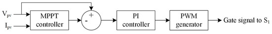
Figure 8. Proposed control algorithm used to control boost converter.

2.2.3. Modelling of Three-Phase Inverter

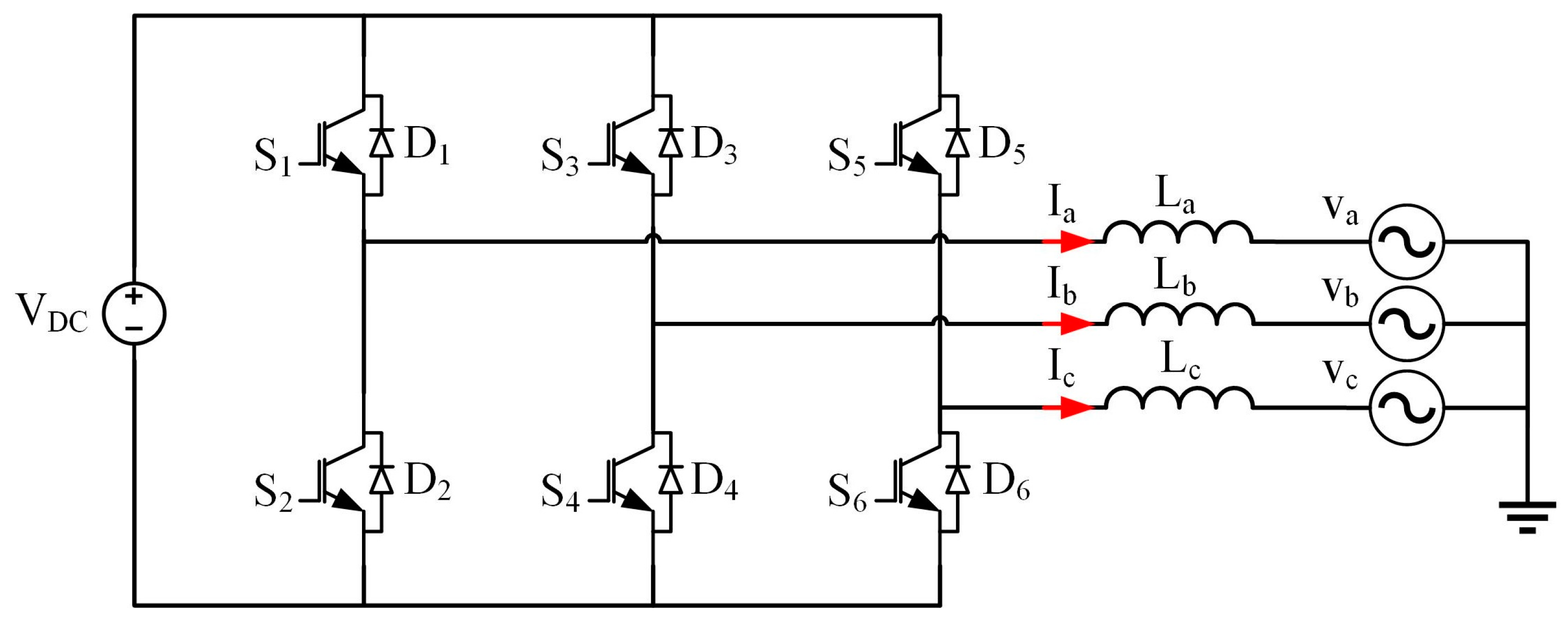
Figure 9 shows the schematic diagram of the three-phase inverter. The proposed design consists of three half-bridge modules connected to three inductors and an AC source to emulate an AC grid. Table 13 provides the switching states for the three-phase inverter.

Figure 9. Proposed topology used in three-phase inverter.

Table 13. Switching states of the three-phase inverter.

S1	S2	S3	S4	S5	S6	Vab	Vbc	Vca	State No
ON	OFF	ON	OFF	ON	OFF	0	0	0	1
OFF	ON	ON	OFF	ON	OFF	−VDC	0	VDC	2
ON	OFF	OFF	ON	ON	OFF	VDC	−VDC	0	3
ON	OFF	ON	OFF	OFF	ON	0	VDC	−VDC	4
ON	ON	OFF	OFF	ON	OFF	0	−VDC	VDC	5
ON	OFF	OFF	ON	OFF	ON	VDC	0	−VDC	6
OFF	ON	ON	OFF	OFF	ON	−VDC	VDC	0	7
OFF	ON	OFF	ON	OFF	ON	0	0	0	8

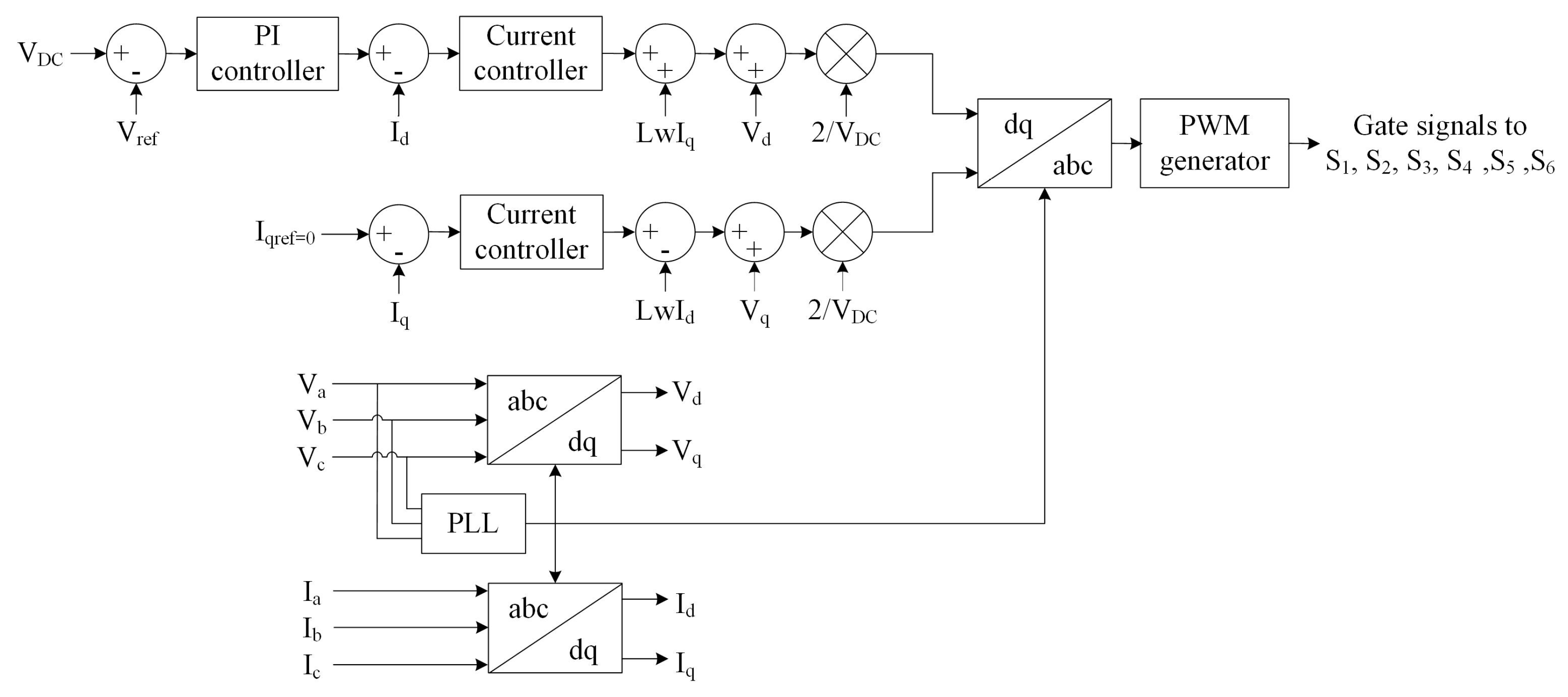
As the input of the three-phase inverter is linked to the DC busbar, it is important to maintain the DC bus voltage. Figure 10 presents the control scheme for the three-phase inverter. This scheme requires voltage and current sensing. The line-to-line voltage from the grid is converted into d–q voltage using Clark’s transformation, and the PLL is implemented with the three-phase grid voltage. The inverter-side current is also transformed into the d–q domain. Here, I_d represents the active current, while I_q corresponds to the reactive current.

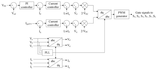
Figure 10. Proposed control algorithm used to control three-phase inverter.

The inverter operates with two control loops: an outer voltage loop and an inner current loop. In the voltage loop, a reference voltage is set to maintain the DC busbar voltage, which is then compared with the measured DC voltage to produce an error signal. This error is processed by a PI controller to generate a reference current I_d, while the reference current I_q is set to zero. In the current loop, the reference I_d and I_q are compared with the actual inverter currents, and the resulting error signals are sent to PI controllers to obtain reference voltages U_d and U_q.

The reference voltage U_d is adjusted by adding the actual V_d and the term LωI_d, where ω is the grid frequency, and L is the filter inductor. Similarly, U_q is adjusted by adding the actual V_q and the term −LωI_q. For the sine PWM scheme, the relationship between the modulation index and inverter voltage is provided in Equations (17) and (18). To obtain the actual V_d and V_q, the reference V_d and V_q are multiplied by ${\displaystyle \frac{{\mathrm{V}}_{\mathrm{DC}}}{2}}$. These are then transformed back to the abc domain to determine the reference duty cycle for PWM generation.

$${\mathrm{V}}_{\mathrm{d}}=\mathrm{md}\times {\displaystyle \frac{{\mathrm{V}}_{\mathrm{DC}}}{2}}$$

(17)

$${\mathrm{V}}_{\mathrm{d}}=\mathrm{mq}\times {\displaystyle \frac{{\mathrm{V}}_{\mathrm{DC}}}{2}}$$

(18)

2.2.4. Assumptions and Limitations of Component Modelling

During the modelling process, certain assumptions were made to focus on key performance metrics and to simplify the analysis:

• Idealized Switching Behavior: It was assumed that the switching devices operate ideally, with no switching losses or parasitic effects. This idealization allows for a clearer understanding of the core dynamics but may not account for all real-world losses.
• Continuous Conduction Mode (CCM): All converters were assumed to operate in CCM, where the current through the inductor never falls to zero. This assumption simplifies the analysis of ripple characteristics and maintains stable operation.
• Thermal Effects and Nonlinearities: The effects of temperature on component performance and nonlinear behaviors (e.g., saturation of inductors) were not included in this stage of the analysis.

3. Simulation Studies

This section presents the simulation of the proposed pico-grid and nano-grid architectures described in Section 3 using MATLAB/Simulink. The models include components such as battery energy storage systems (BESSs), single-phase inverters, solar PV boost converters, and three-phase inverters. The DC and AC loads are modelled based on the load demand estimations provided in Section 2. Various test conditions are simulated to reflect real-time scenarios.

3.1. Simulation of Pico-Grid System

The pico-grid system is modelled in MATLAB/Simulink to simulate various test conditions based on real-time scenarios. Each BESS in the pico-grid system can provide up to 10 kW of power to both DC and AC loads, with the power reference set using the Iref parameter in the BESS control algorithm. The DC link voltage of the DC busbar is maintained at 400 V using the single-phase inverter’s outer voltage loop control algorithm. The output of the single-phase inverter is connected to the single-phase grid. The parameters of the proposed pico-grid system are shown in two tables: Table 14 shows the BESS parameters, and Table 15 shows the single-phase inverter and grid parameters used in this simulation.

Table 14. Parameters of BESS for pico-grid system.

Parameters	Value
Battery nominal voltage	Vbatt = 48 V
Battery rated capacity	Ibatt = 300 Ah
Initial SOC	SOC = 45%
Switching frequency	Fsw = 10 kHz
Inductor value	L = 2.5 mH

Table 15. Parameters of single-phase inverter for pico-grid system.

Parameters	Value
Switching frequency	Fsw = 5 kHz
Filter inductor	L = 2.5 mH
Filter capacitor	C = 1000 µF
DC link voltage	VDC = 400 V
Distribution grid voltage	Vgrid = 230 V (phase)

The selection of parameters, such as inductor values, capacitor sizes, and switching frequencies, was based on achieving a balance between system performance, efficiency, and stability. The inductor was sized to limit the ripple current to 20–40% of the rated output current, minimizing losses while maintaining output voltage stability. For example, in the case of the BESS, using Equation (4), with an input voltage of 48 V, a duty cycle of 0.5, a switching frequency of 20 kHz, and a desired ripple current of 10 A, the calculated inductor value is approximately 0.04 mH. Similarly, the capacitor value of the inverter was determined using Equation (6) to ensure a voltage ripple of 1–5% of the DC bus voltage. For a 400 V DC bus with an output current of 200 A, a duty cycle of 0.5, and a switching frequency of 5 kHz, the calculated capacitor value is approximately 1000 μF, which was selected to maintain voltage stability.

The choice of switching frequency balanced efficiency, ripple suppression, and thermal considerations. Higher switching frequencies reduce current ripple but increase switching losses and heat generation, while lower frequencies enhance efficiency but can increase output ripple. A frequency of 20 kHz was selected to achieve a balance suitable for the given converter size and thermal design.

It is important to note that the actual values used in the simulation as shown in Table 14 and Table 15 differ slightly from the theoretical calculations. During the simulation process, some variations in performance were observed, prompting adjustments to the parameter values to achieve desired outcomes and ensure the stability and accuracy of the results.

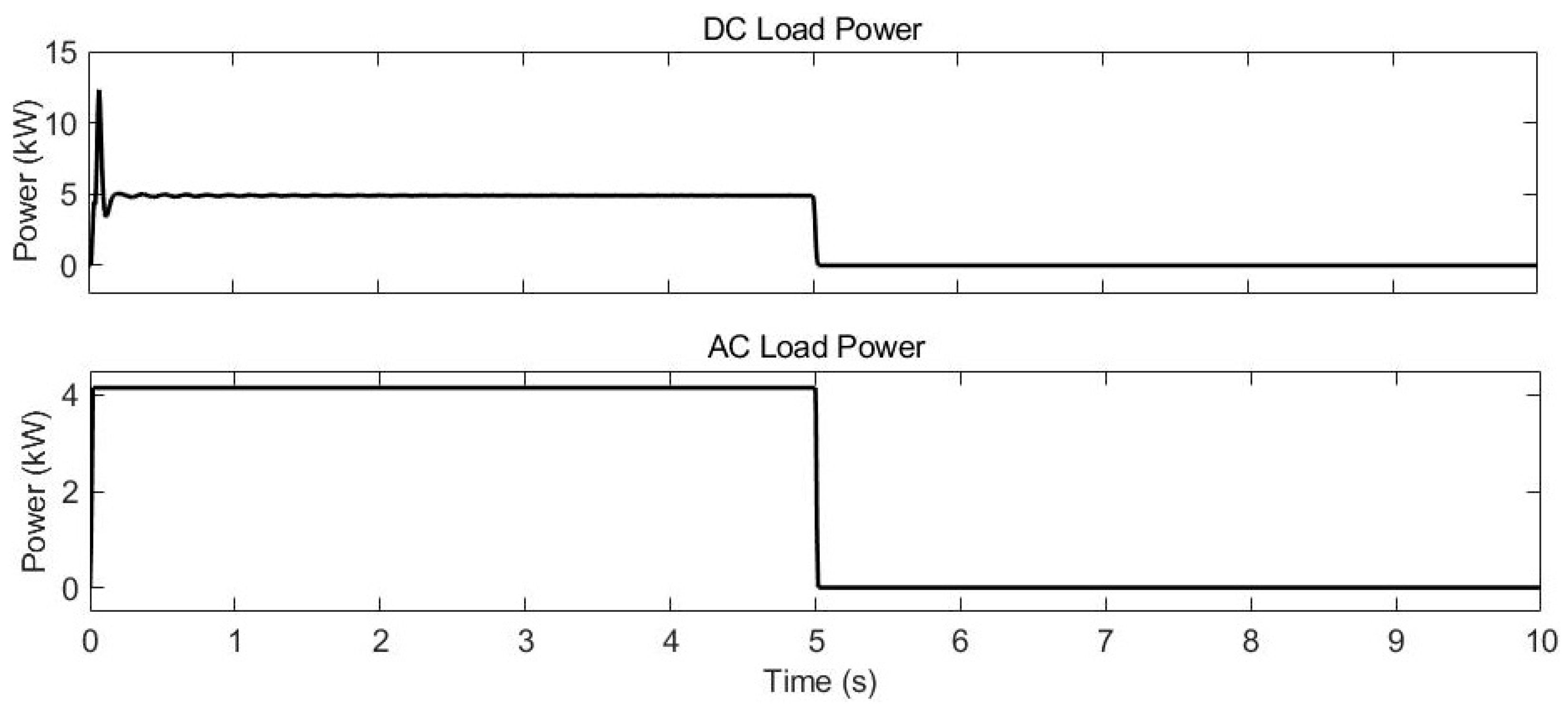
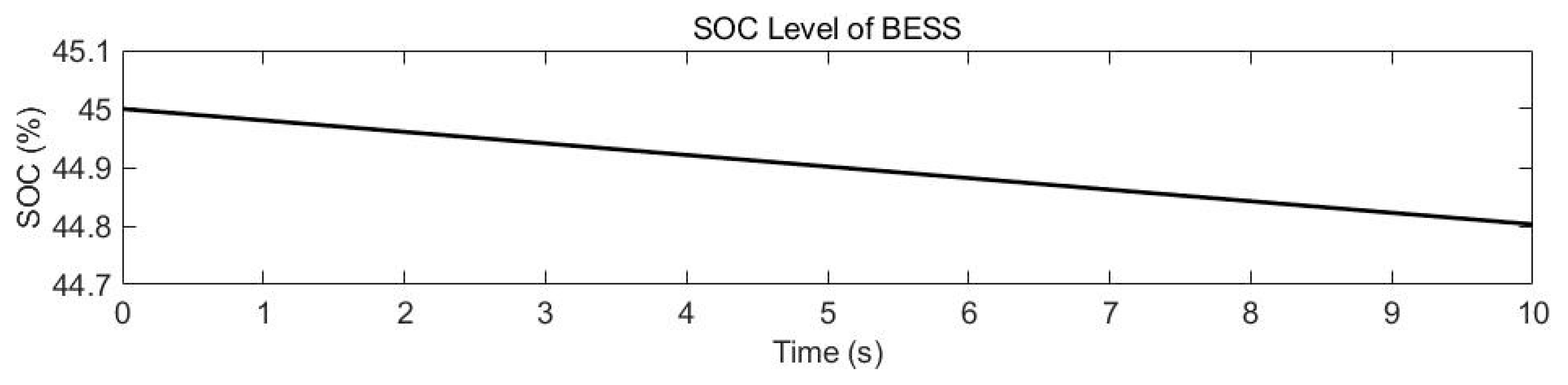
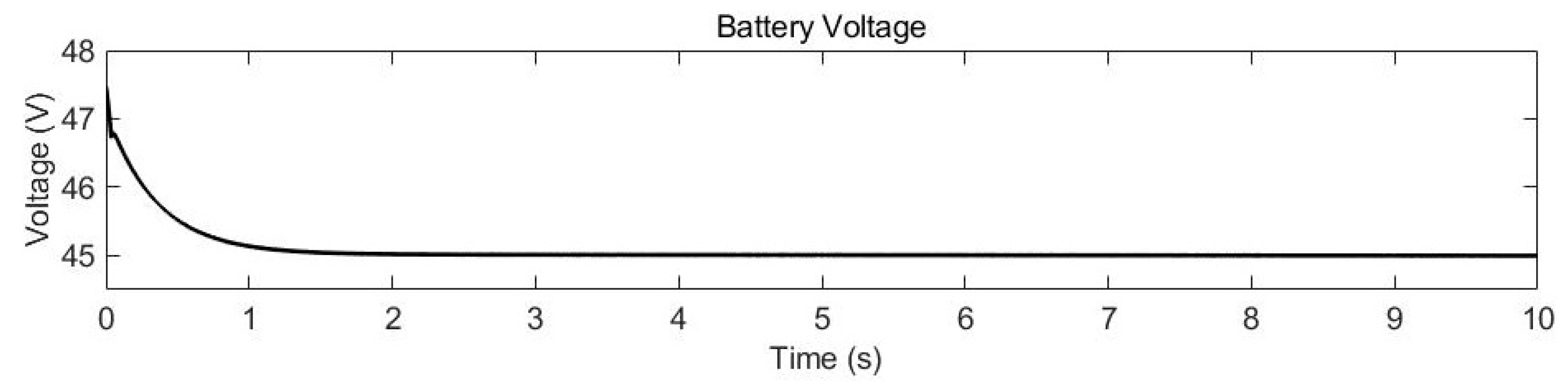
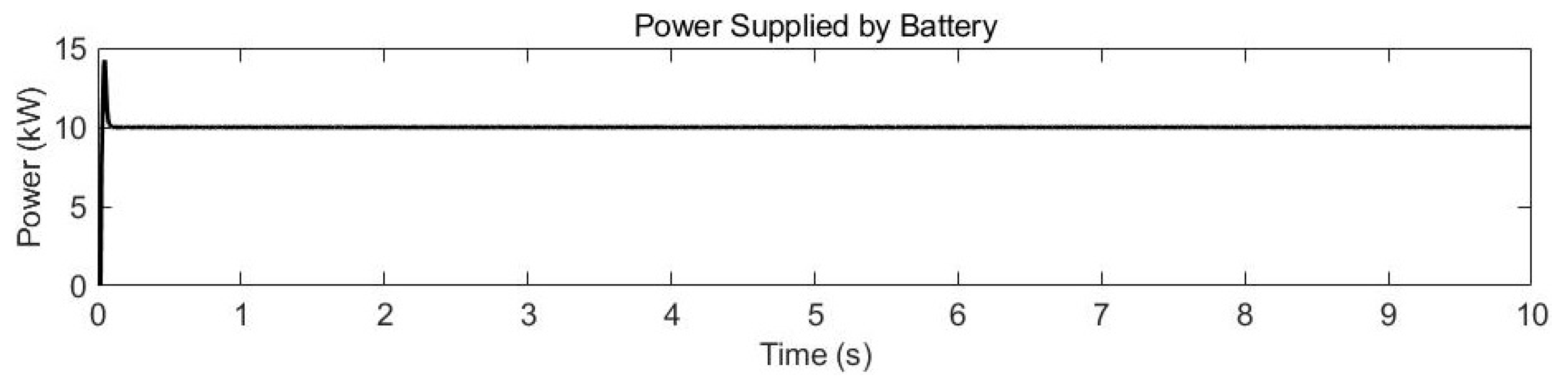
To integrate the BESS with a single-phase inverter, the load demand estimated in Section 2 for each individual level is utilized in this simulation to demonstrate the system’s operation. Figure 11 shows the simulation model for this integration. In this scenario, the DC load is set at 4900 W, and the AC load at 4150 W, as shown in Figure 12. The simulation focuses on discharging the battery to supply both DC and AC loads. The battery begins with a state of charge (SOC) of 45%, which decreases as the battery discharges, as shown in Figure 13. During discharge, the battery voltage drops from 48 V to 45 V, as shown in Figure 14, and the battery current tracks the reference current, as shown in Figure 15. The battery has a capacity of 10 kW, as shown in Figure 16.

Figure 11. Simulation model of BESS integration with single-phase inverter.

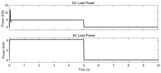
Figure 12. Load demand estimation of DC (top) and AC (bottom) loads for pico-grid system.

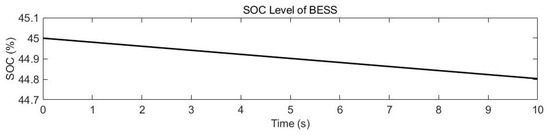
Figure 13. The SOC level of the BESS during discharging in pico-grid system.

Figure 14. The battery voltage of the BESS during discharging in pico-grid system.

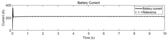
Figure 15. Battery current of BESS during discharging in pico-grid system.

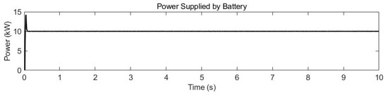
Figure 16. Battery capacity of BESS during discharging in pico-grid system.

The battery’s input voltage is stepped up to 400 V, which is fed into the DC busbar, as shown in Figure 17. The single-phase inverter then converts this 400 V DC into 230 V AC for grid connection. With a total load demand of 9050 W and a system capacity of 10 kW, any surplus power can be exported to the grid, as shown in Figure 18.

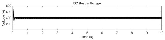
Figure 17. Voltage level at DC busbar in pico-grid system.

Figure 18. Surplus power delivered to the grid in pico-grid system.

3.1.1. Test Condition 1: Battery Charging at Night

The simulation model shown in Figure 11 is used to simulate the process of charging the BESS from the grid during nighttime hours, when grid power is available at lower tariffs, and the load demand is reduced. Charging the battery at night is advantageous as it leverages off-peak electricity tariffs and reduces the load on the utility grid, making the pico-grid operation more efficient and cost-effective.

In this simulation, the BESS begins with a SOC of 45%, which gradually increases as the battery absorbs energy from the grid, as shown in Figure 19. Figure 20 shows that as the SOC increases, the battery voltage also rises from about 47.45 V to about 48.2 V, which is close to its nominal level, demonstrating a smooth charging process. Throughout the charging period, the DC busbar voltage is maintained at 400 V, as shown in Figure 21, ensuring the system remains stable. The BESS operates in buck mode, stepping down the voltage to 48 V to match the battery’s nominal charging voltage, supporting the system’s ability to balance load demands and maintain consistent power flow during energy storage operations.

Figure 19. SOC level of the BESS during charging in pico-grid system.

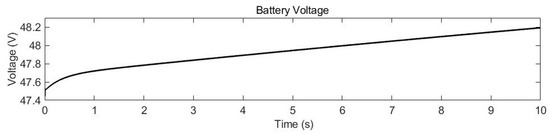
Figure 20. Battery voltage of the BESS during charging in pico-grid system.

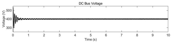
Figure 21. DC bus voltage of the BESS during charging in pico-grid system.

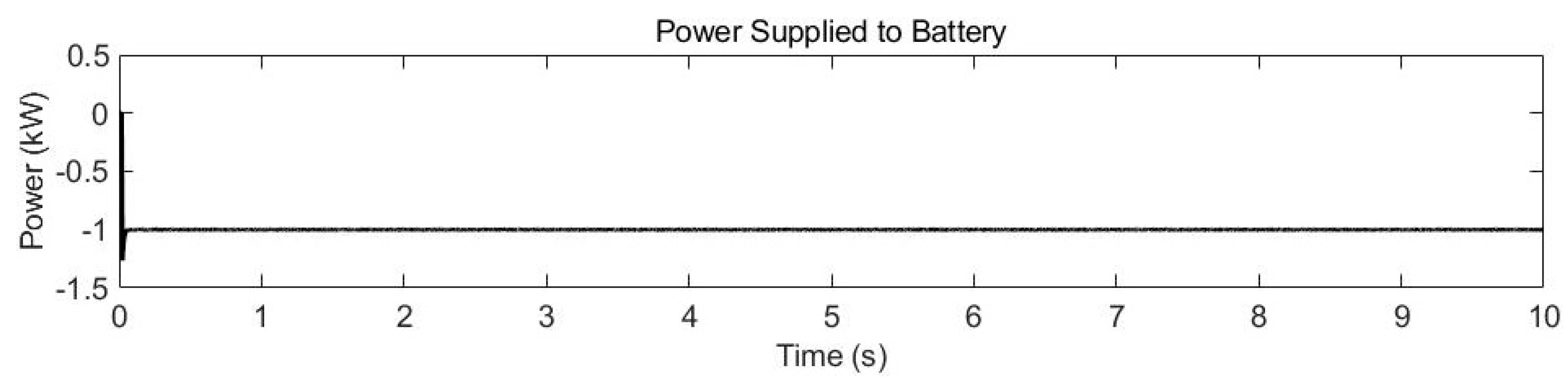
The power reference for this simulation is set at −1 kW, meaning the battery is configured to receive 1 kW of power for charging. The battery current adjusts accordingly, following the reference current as it charges, as shown in Figure 22. The consistent power flow from the grid is used to charge the battery, with the grid supplying 1 kW of power, which the battery stores for future use, as shown in Figure 23. The steady increase in the battery’s SOC and voltage, as observed in the simulation, demonstrates the proper functioning of the BESS inverter controller.

Figure 22. Battery current of BESS during charging in pico-grid system.

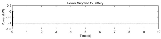
Figure 23. Battery capacity of BESS during charging in pico-grid system.

The results show that the charging process is stable and controlled, with a gradual increase in the battery’s SOC, typical of a nighttime charging scenario. The rise in battery voltage from about 47.45 V to about 48.2 V as seen in Figure 20, follows the design of the charging algorithm, demonstrating that the system can effectively manage power flow and grid interaction during off-peak hours. The key advantage of nighttime charging is the reduced cost due to lower tariffs, as well as a more balanced load on the grid, making the operation not only economical but also efficient for grid management. Additionally, Figure 24 shows the supplying of power from the grid to charge the battery during this process, highlighting the grid’s role in supporting the battery’s energy needs during off-peak hours.

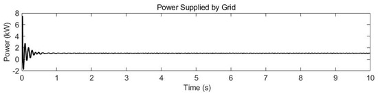
Figure 24. Supplying power from the grid to charge the battery in pico-grid system.

3.1.2. Test Condition 2: Rainy Day Operation

In this simulation, two pico-grid models are connected in parallel and linked to a single-phase grid to analyze the power flow between two levels of a building, as shown in Figure 25. The load demand for each level, as previously estimated, is used to demonstrate system operation. Levels 1 and 2 of the building are selected for this power flow analysis, with the simulation assuming a DC load of 4900 W and an AC load of 4150 W at for 0 ≤ t < 5 s, as shown in Figure 26. During the initial time interval for 0 ≤ t < 5 s, both levels have identical DC and AC loads. The system is balanced, with each level generating sufficient power to meet its own demand. The batteries on each level supply the load requirements, and the surplus power of about 1800 kW generated is exported to the grid as shown in Figure 27.

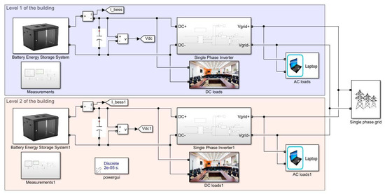
Figure 25. Two parallel pico-grids connected to the single-phase grid.

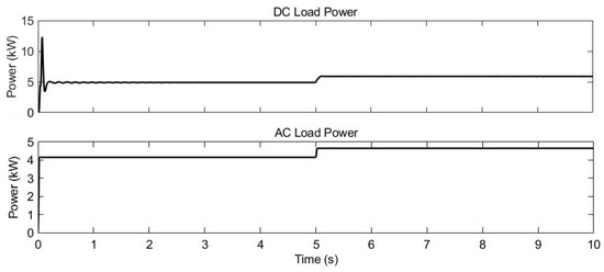
Figure 26. DC (top) and AC loads (bottom) of two pico-grids system.

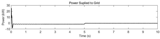
Figure 27. Surplus power from the system sent to the grid for two pico-grids system.

During rainy conditions, the pico-grid adapts dynamically by drawing power from the grid when local generation is insufficient. As shown in Figure 26, the system maintains a steady output voltage of 230 V AC and ensures that the increased load on Level 2 is supported through power sharing. The power exported to the grid drops from 1800 W to 300 W, as shown in Figure 27, demonstrating the system’s real-time load balancing capability.

At t = 5 s, the load demand on level 2 is increased, with the DC load and the AC load increasing to 5900 W and 4650 W respectively, as shown in Figure 26. This sudden increase in demand on level 2 exceeds the power generated by its battery, necessitating a transfer of power from level 1 to meet the increased load on level 2. Since both levels are connected in parallel to the single-phase grid, the system dynamically redirects surplus power from level 1 to support the increased load on level 2.

As a result of this power transfer, the surplus power that was initially being exported to the grid decreases to only about 300 W for 5 ≤ t < 10 s, as shown in Figure 27. Prior to the increase in load demand, both levels were generating surplus power for grid export. After the load spike on level 2, the system prioritizes local demand, thus reducing the power exported to the grid. This demonstrates the pico-grid’s ability to adapt to real-time changes in power demand, efficiently managing both internal loads and external grid interaction.

3.2. Simulation of Nano-Grid System

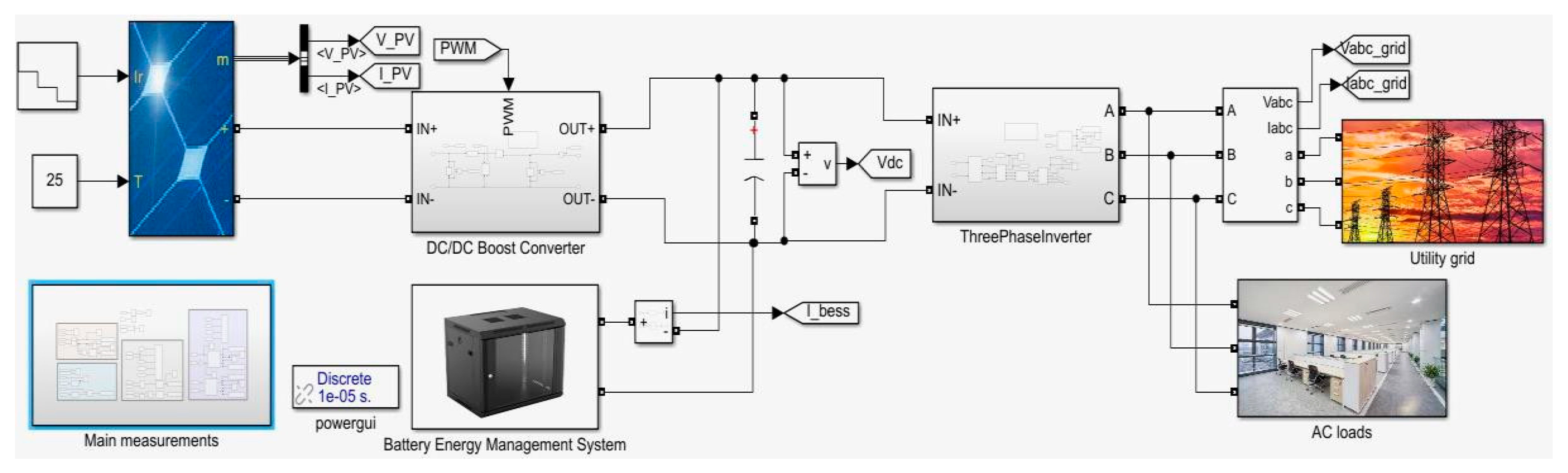
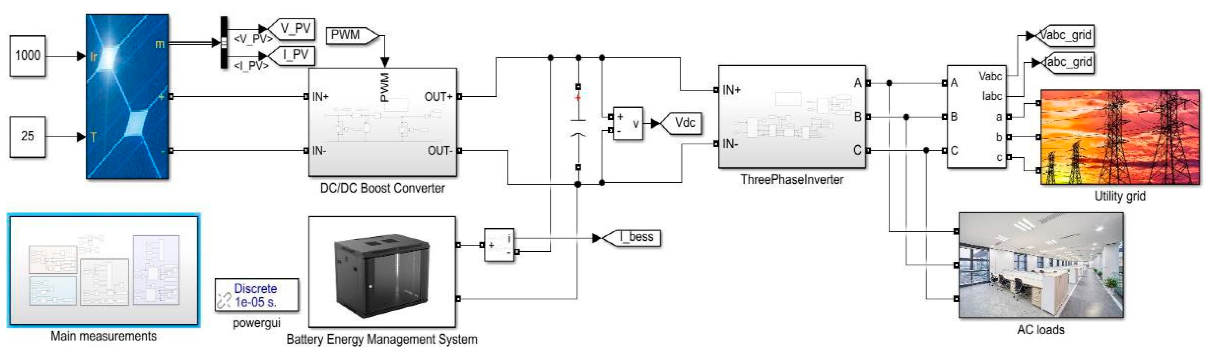
The nano-grid system was modelled in MATLAB/Simulink to simulate various test scenarios based on real-world conditions. In this setup, the solar PV system is designed to generate 40 kW of power, while the BESS can provide an additional 10 kW to meet both DC and AC load demands. The solar PV panels are connected to a boost converter, which steps up the input voltage from 400 V to 1000 V at the DC busbar. The DC link voltage of the busbar was maintained at 1000 V using the outer voltage loop control algorithm of the three-phase inverter. The power reference for the BESS was determined by the I_ref in the proposed BESS control algorithm.

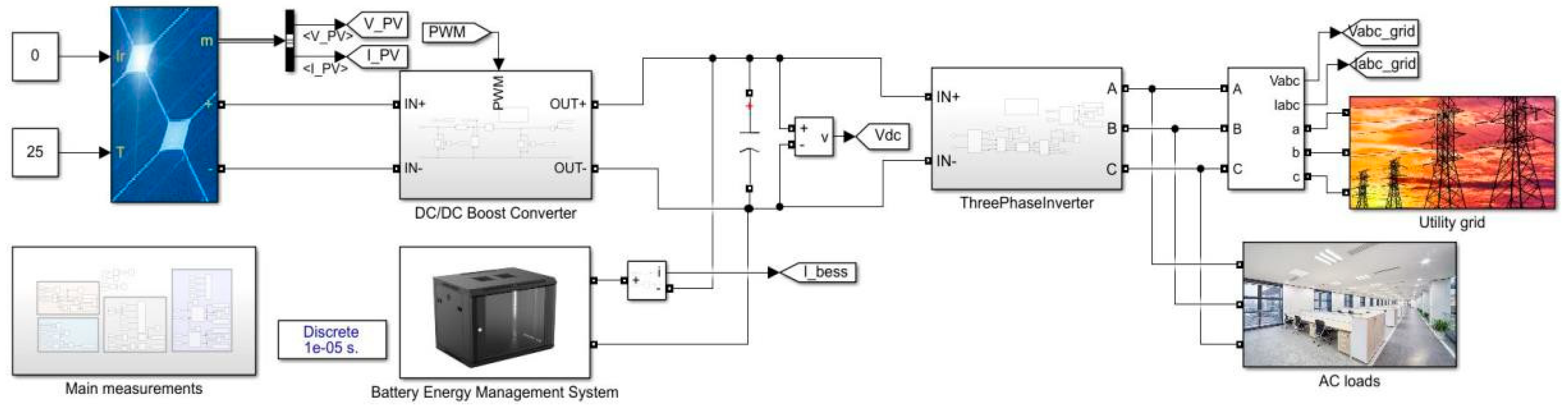
The parameters of the nano-grid system are detailed in four tables: Table 16 lists the solar PV system parameters, Table 17 details the boost converter parameters, Table 18 outlines the BESS parameters, and Table 19 provides the three-phase inverter and grid parameters. Figure 28 shows the integration of the solar PV system, BESS, and three-phase inverter.

Table 16. Parameters of solar PV system for nano-grid system.

Parameters	Value
Series-connected strings	10
Parallel-connected strings	10
Vmp	Vmp = 40.8 V
Imp	Imp = 9.81 A
Sun irradiance	Ir = 1000 W/m2
Cell temperature	T = 25 °C

Table 17. Parameters of boost converter for nano-grid system.

Parameters	Value
Switching frequency	Fsw = 5 kHz
Inductor value	L = 2.5 mH
Input capacitor value	Cin = 1000 µF
Output capacitor value	Cout = 4000 µF

Table 18. Parameters of BESS for nano-grid system.

Parameters	Value
Battery nominal voltage	Vbatt = 400 V
Battery rated capacity	Ibatt = 300 Ah
Initial SOC	SOC = 45%
Switching frequency	Fsw = 10 kHz
Inductor value	L = 1 mH

Table 19. Parameters of three phase inverter.

Parameters	Value
Switching frequency	Fsw = 10 kHz
Inductor value	L = 10 mH
DC link voltage	VDC = 1000 V
Distribution grid voltage	Vgrid = 400 V (line)

Figure 28. Simulation model of integration of solar PV and BESS with three-phase inverter.

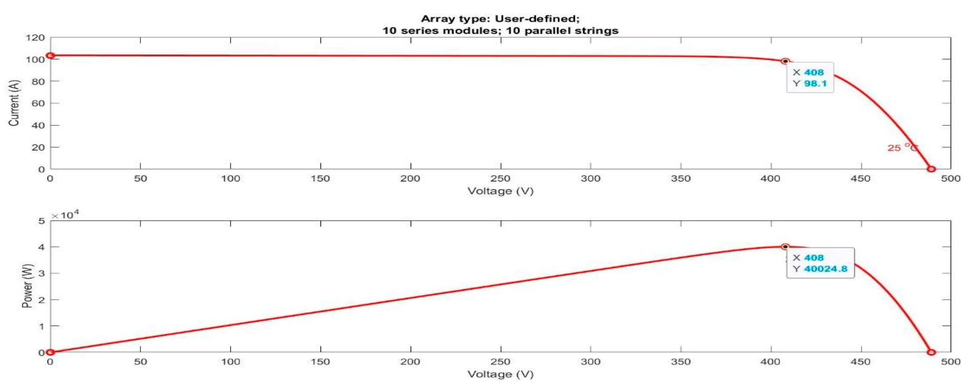
The load demand estimated in Section 2 was used in this simulation to demonstrate the system’s operation. The solar PV array consists of 10 series-connected and 10 parallel-connected modules, producing a total of 40 kW, as shown in Figure 29. The AC load in the simulation was set to 40 kW, as shown in Figure 30, with both the solar PV and BESS supplying the AC loads.

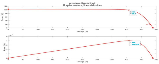
Figure 29. Solar PV array waveform.

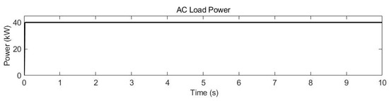
Figure 30. Load demand estimation of AC loads in nano-grid system.

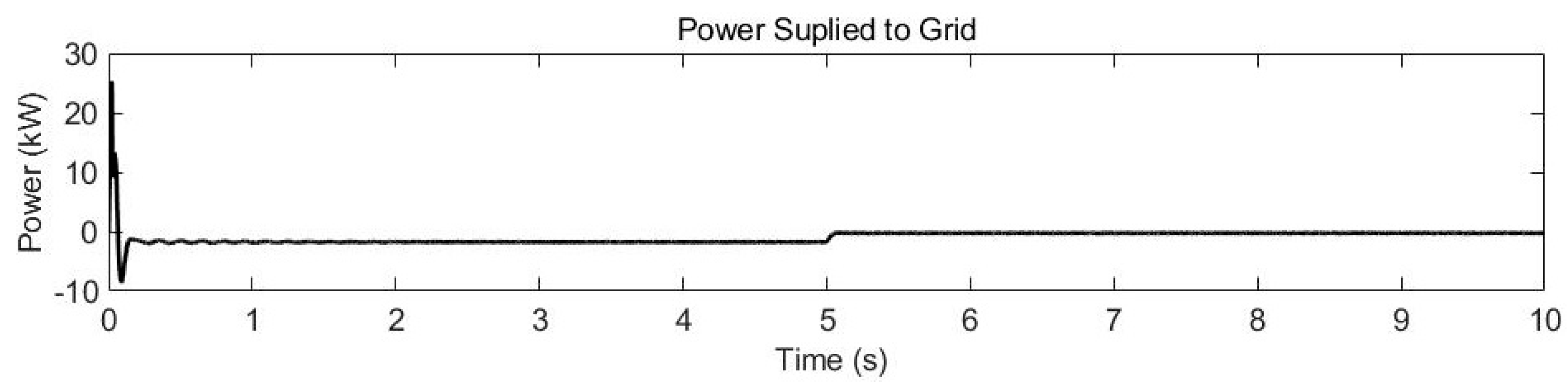
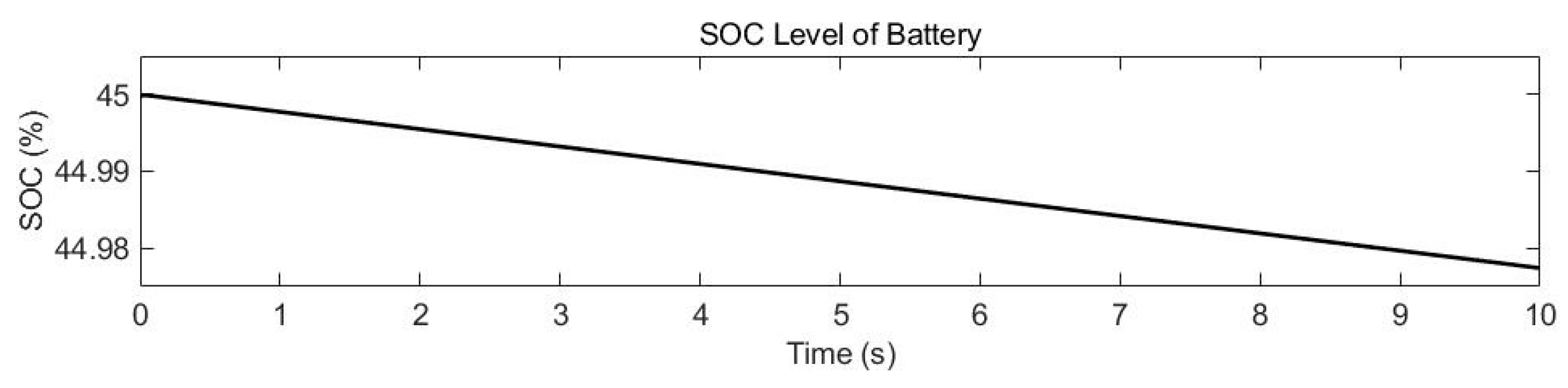
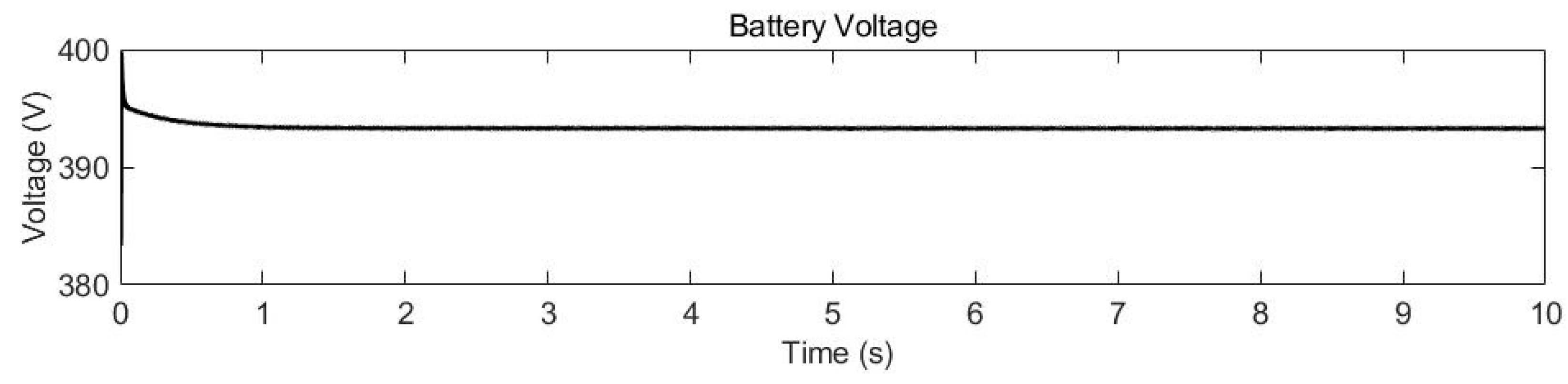
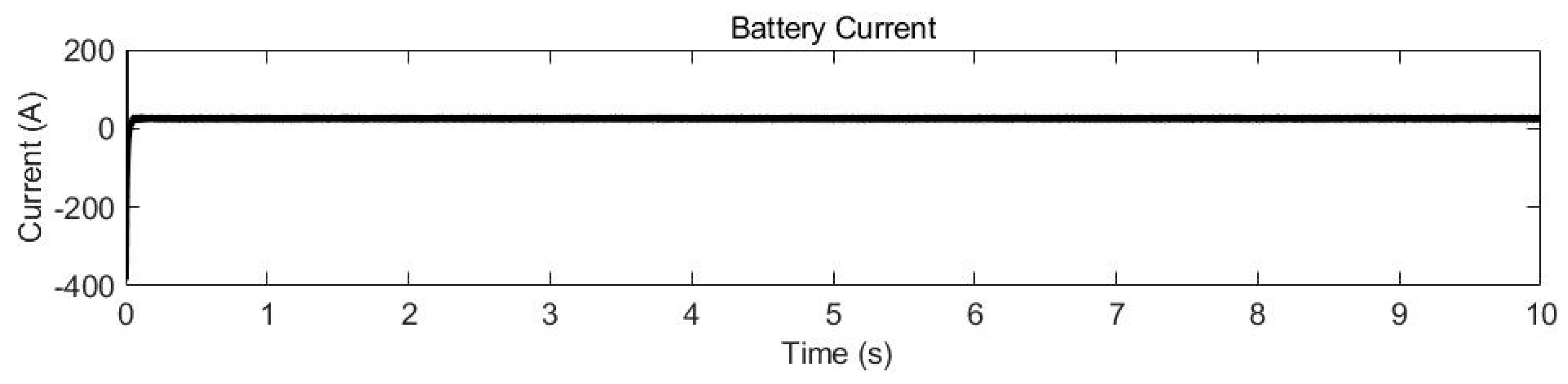
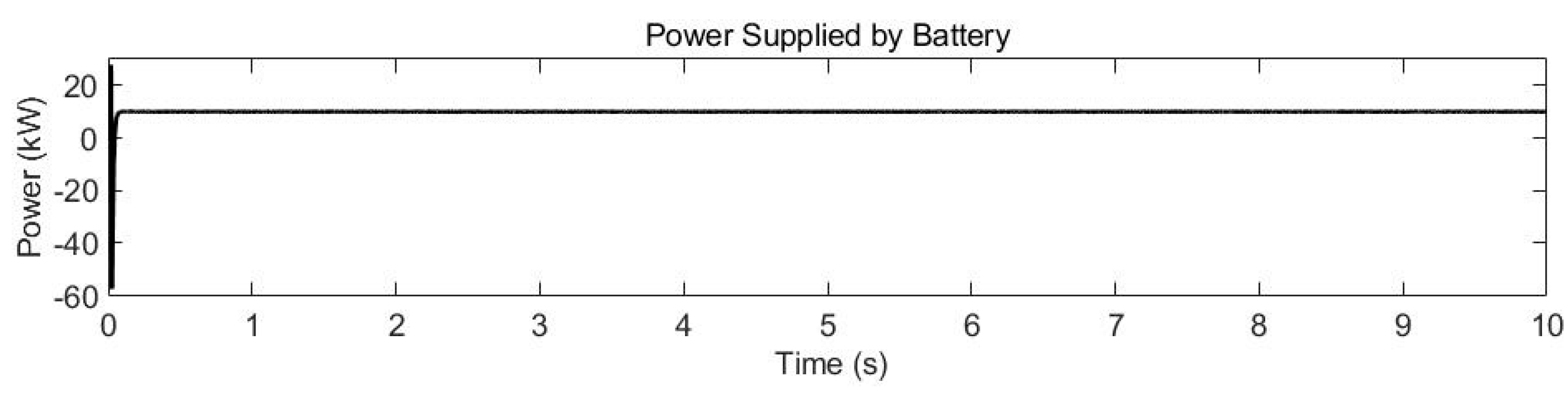
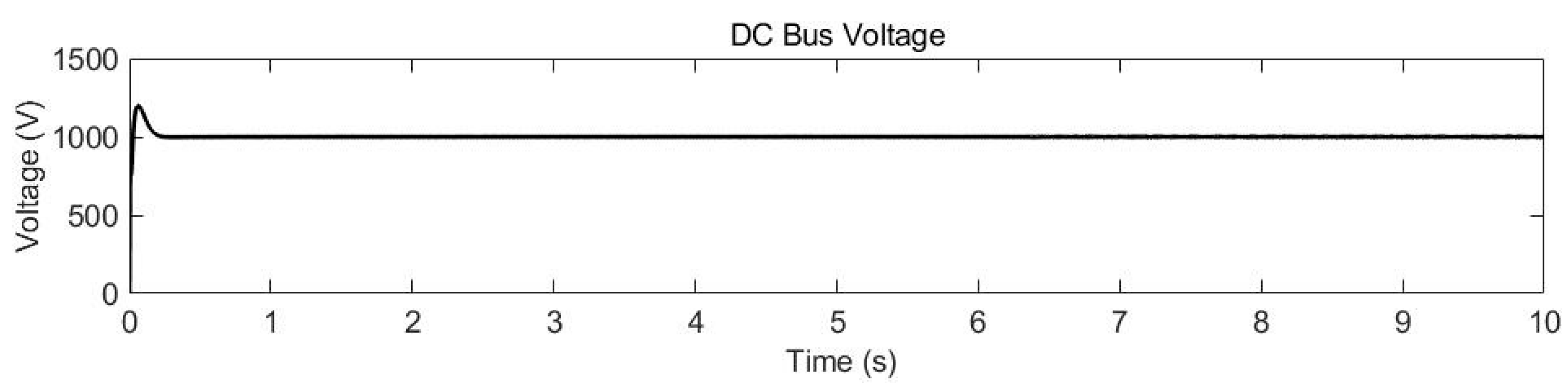
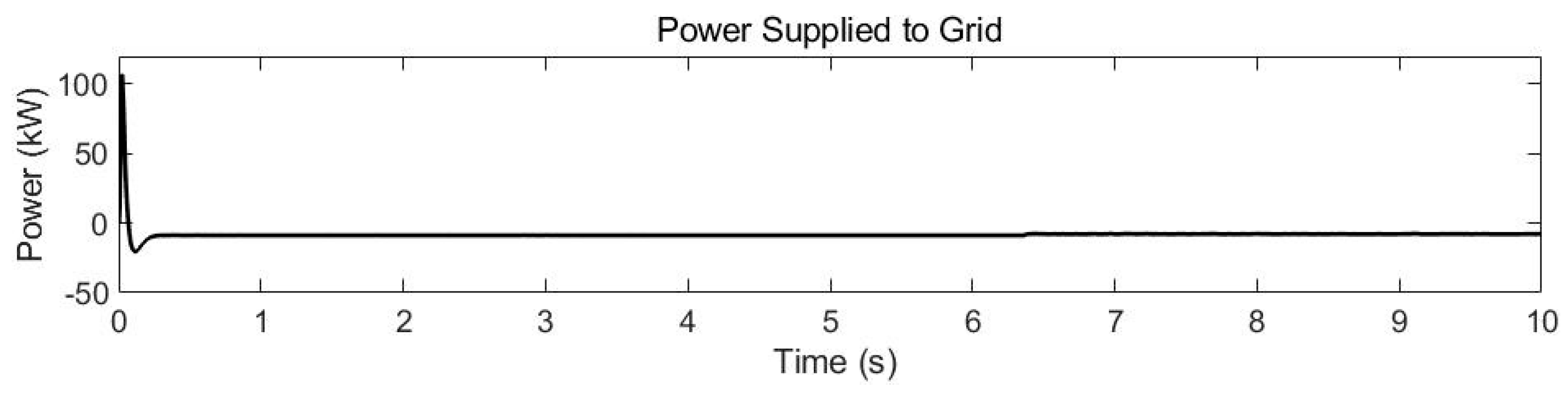
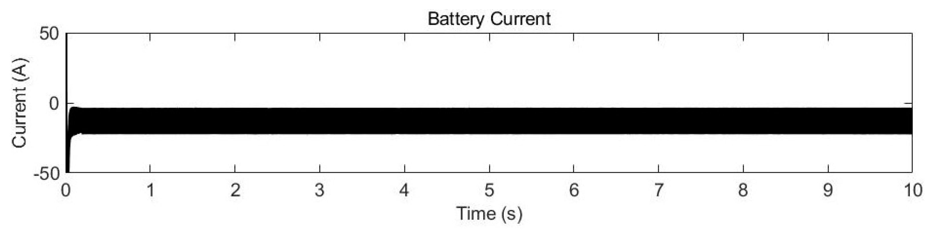
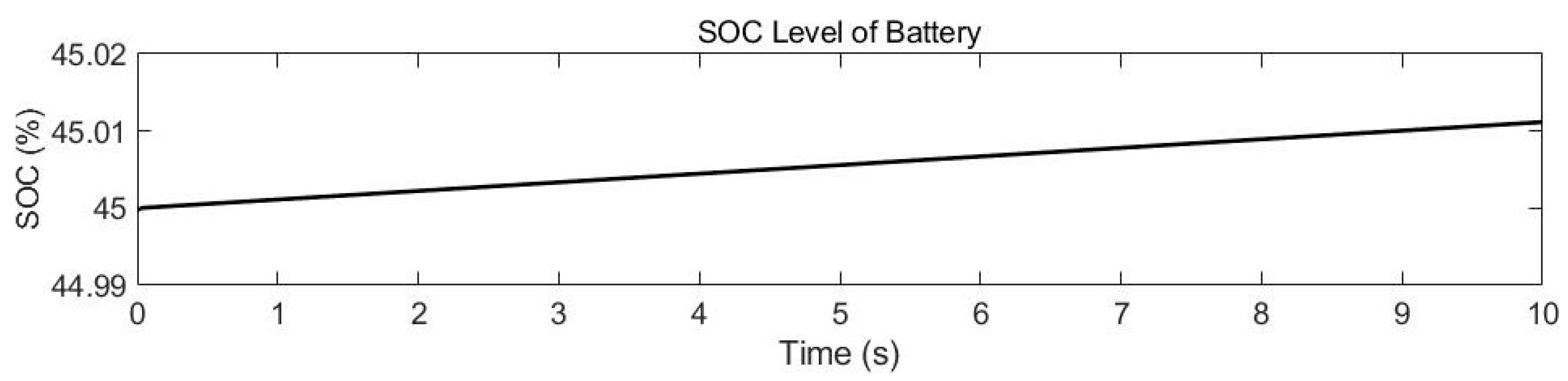
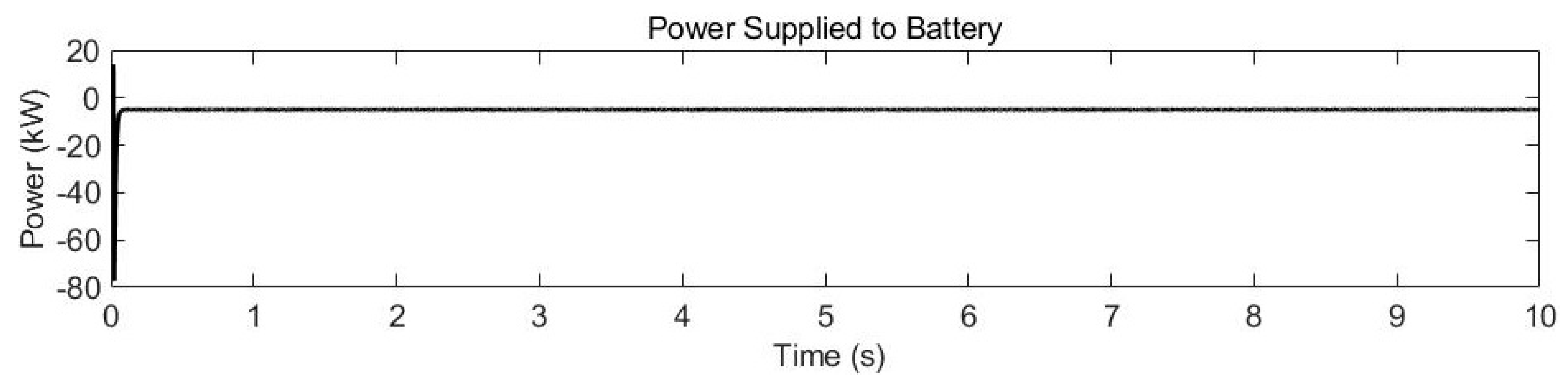
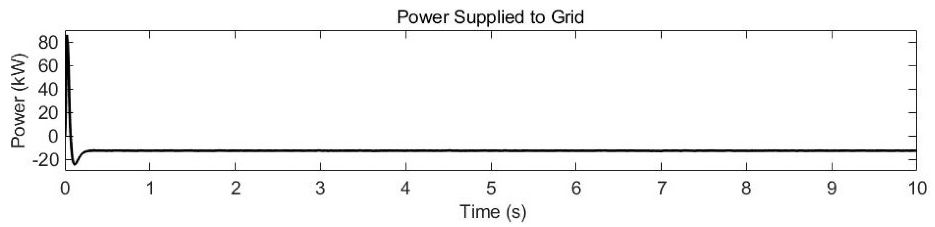
The solar PV panels are connected to a boost converter that raises the voltage from 400 V to 1000 V at the DC busbar. The battery starts with an SOC of 45%, which gradually decreases as it discharges to supply the load, as shown in Figure 31. During discharging, the battery voltage drops from 400 V to 390 V, as shown in Figure 32, and the battery current aligns with the reference current, as seen in Figure 33. The battery’s capacity was set to 10 kW, as shown in Figure 34. The battery’s input voltage was stepped up to 1000 V at the DC busbar, as shown in Figure 35. The 1000 V DC from the busbar was then inverted to 400 V AC by the three-phase inverter, which is connected to the grid. With a load demand of 40 kW and a combined power generation of 50 kW from the solar PV and BESS, the excess power can be exported to the grid, as shown in Figure 36.

Figure 31. SOC of battery during discharging in nano-grid system.

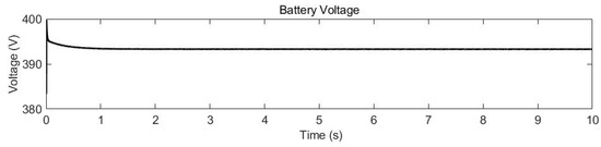
Figure 32. Battery voltage of the BESS during discharging in nano-grid system.

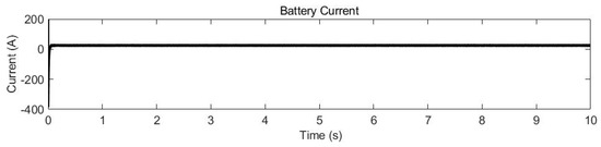
Figure 33. Battery current of BESS during discharging in nano-grid system.

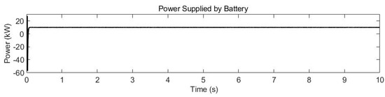
Figure 34. Power supplied by battery of BESS during discharging in nano-grid system.

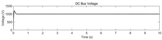
Figure 35. Voltage level at DC busbar in nano-grid system.

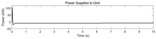
Figure 36. Surplus power delivered to the grid in nano-grid system.

3.2.1. Test Condition 1: Charging of Battery at Night

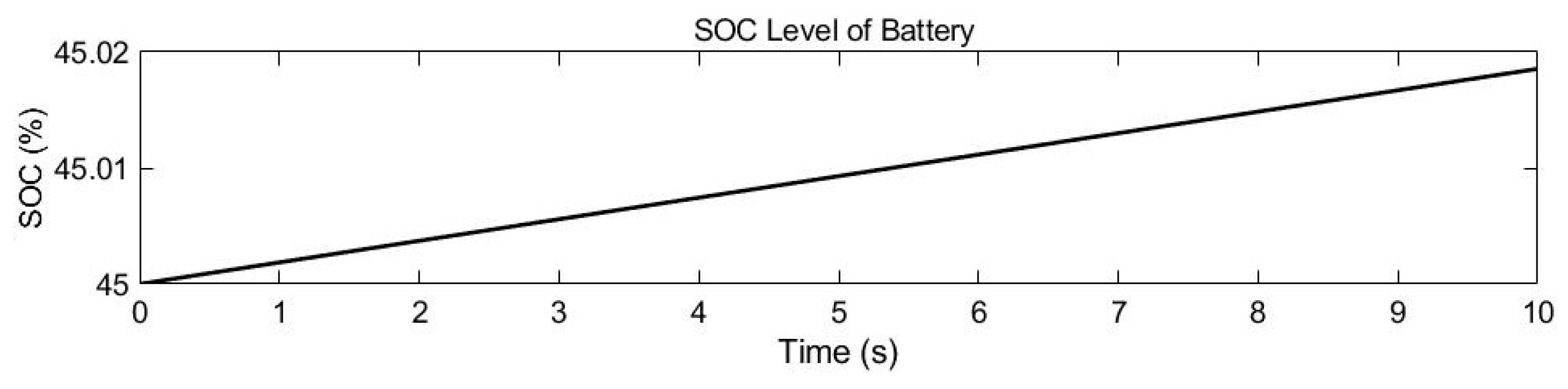
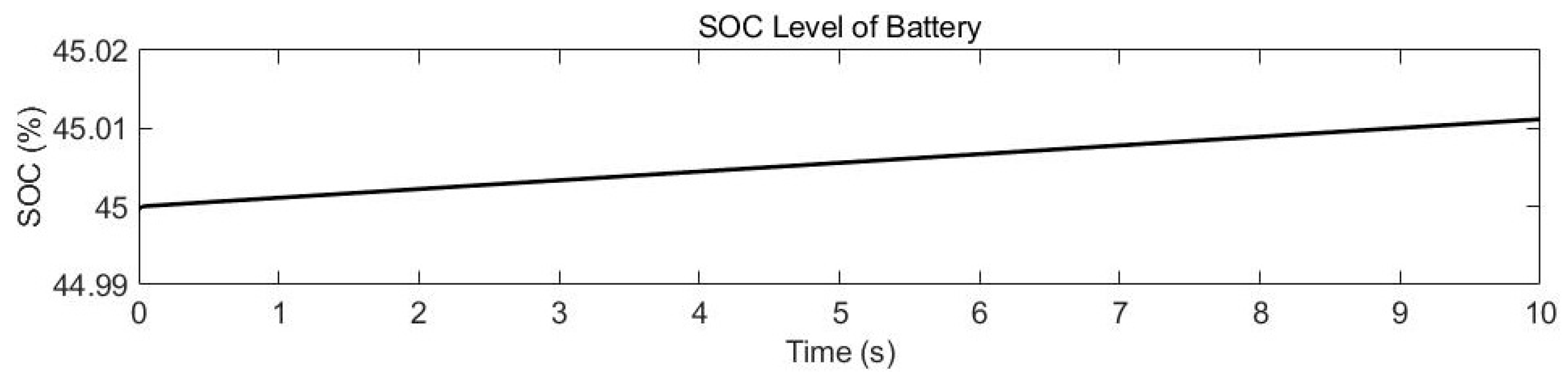
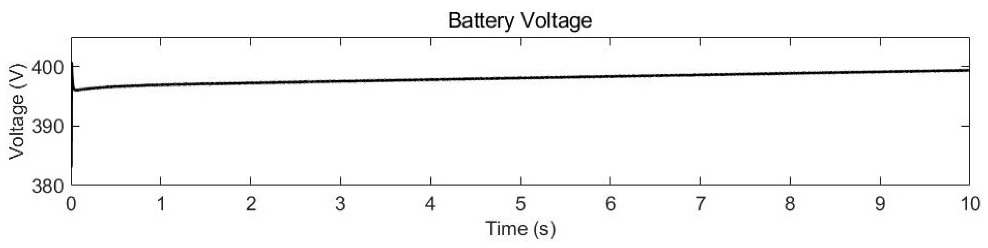
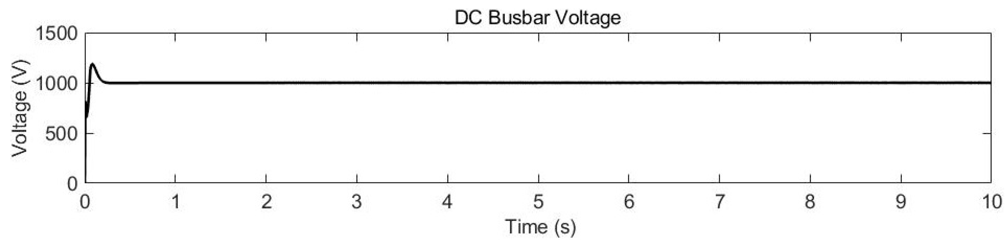
The simulation model shown in Figure 37 was used to simulate the battery charging process from the grid during nighttime hours, capitalizing on the advantages of lower load demands and cheaper electricity tariffs. This test scenario demonstrates the benefits of using grid power to charge the battery under conditions that favor energy storage. The battery starts with an initial SOC of 45%, which gradually increases as the charging progresses, as shown in Figure 38. During this process, the battery voltage rises from 396 V to its nominal level of 398 V, as shown in Figure 39, reflecting a smooth and controlled charging process that aligns with the designed charging algorithm. The nano-grid operates efficiently in buck mode while charging its battery from the grid. Figure 38 shows that the SOC increases steadily from 45% to 90%, while the DC bus voltage remains stable at 1000 V, as shown in Figure 40. This consistent behavior supports the assertion of smooth transitions under grid-connected conditions.

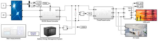
Figure 37. Simulation model to demonstrate charging of battery.

Figure 38. SOC of battery during charging in nano-grid system.

Figure 39. Battery voltage of the BESS during charging in nano-grid system.

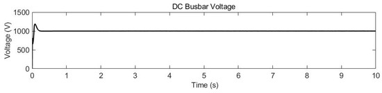
Figure 40. Voltage level at DC busbar in nano-grid system (Test Condition 1).

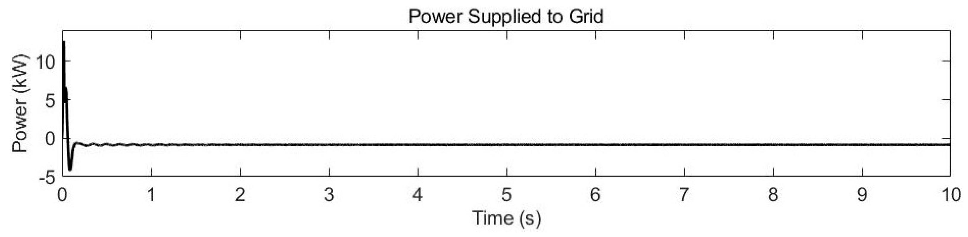
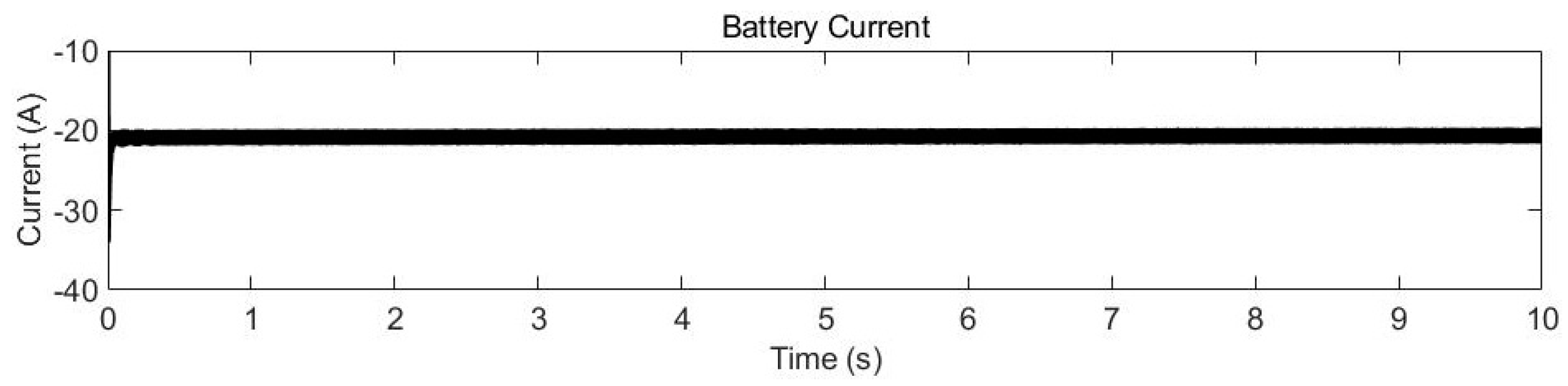
Throughout the charging operation, the DC busbar voltage was kept stable at 1000 V, as shown in Figure 40, which is crucial for ensuring system-wide stability. The BESS (BESS) functions in buck mode, stepping down the voltage to 400 V to match the battery’s charging requirements. The power reference for the BESS was set at −5 kW, indicating that the battery is controlled to receive 5 kW of power. The battery current adjusts accordingly, following this reference throughout the charging, as shown in Figure 41, while the consistent power flow of 5 kW supplied by the grid confirms that the system is effectively in charging mode. The grid’s role in supporting the battery’s energy needs is evident, as shown in Figure 42, with the energy drawn from the grid clearly shown in Figure 43.

Figure 41. Battery current of BESS during charging in nano-grid system.

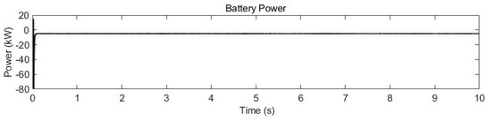
Figure 42. Battery capacity of BESS during charging in nano-grid system.

Figure 43. Drawing power from the grid to charge the battery in nano-grid system.

The charging process is demonstrated to be stable and well-regulated, with a gradual increase in the battery’s SOC being characteristic of a nighttime charging scenario, where cost and efficiency benefits are maximized due to lower electricity tariffs and reduced grid stress. The 2 V rise in battery voltage from 396 V to 398 V, seen in Figure 39, shows that the charging dynamics are steady and within the optimal range to preserve battery health. By maintaining a smooth voltage increase, the system reduces the likelihood of overvoltage conditions, which could otherwise lead to overheating or affect the lifespan of the battery.

3.2.2. Test Condition 2: Operation During Rainy Day

The simulation model shown in Figure 44 was used to evaluate the system performance when solar irradiance decreases due to rainfall. This test scenario demonstrates how the nano-grid adapts when solar energy generation is significantly reduced, and both the BESS and the grid must supply the load.

Figure 44. Simulation model to demonstrate a rainy-day operation.

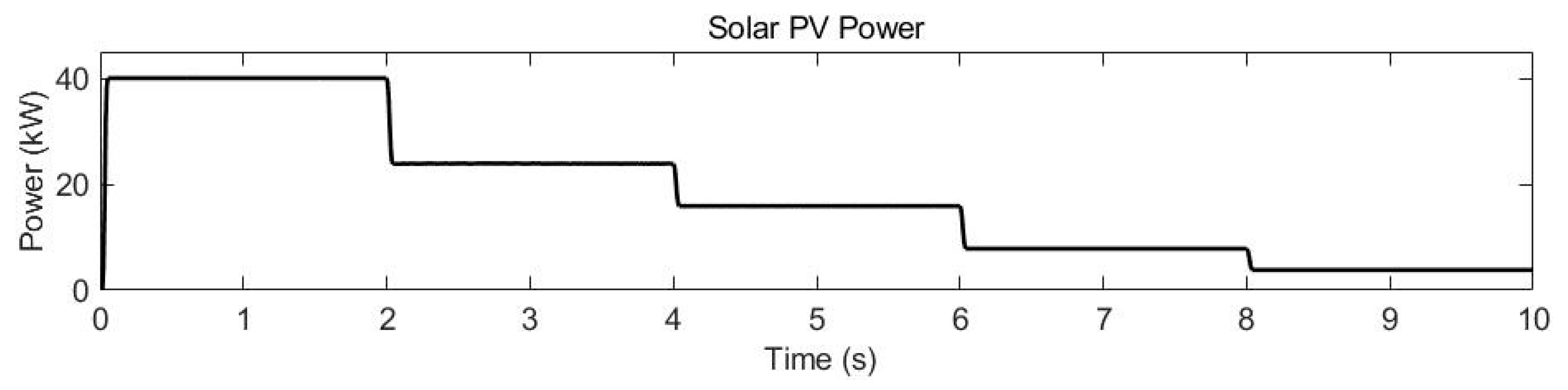
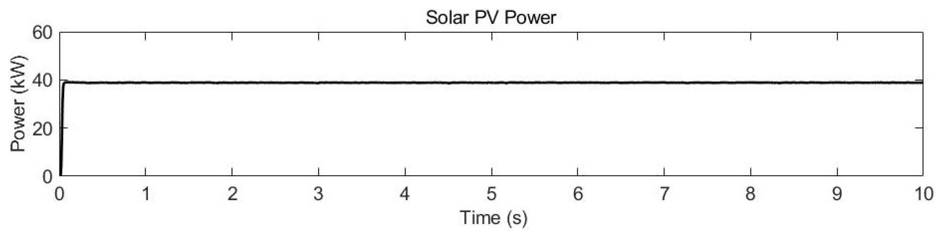
Initially, during the time interval 0 ≤ t < 2 s, the solar irradiance is 1000 W/m², allowing the solar PV system to generate 40 kW of power, as shown in Figure 45. At this stage, the solar PV system alone can meet the AC load demand of 40 kW, shown in Figure 46, without any contribution from the grid. During this period, the system operates efficiently, leveraging solar energy to fully support the load. This demonstrates the grid-support functionality and the nano-grid’s ability to maintain operational stability.

Figure 45. Solar PV power in nano-grid system.

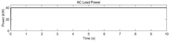
Figure 46. Load demand of AC loads in nano-grid system.

However, at t = 2 s, the irradiance drops to 800 W/m², reducing the solar PV output to 24 kW. This decrease in solar generation results in a shortfall, as the combined power from the solar PV and BESS (which was set to supply 10 kW) is now insufficient to meet the 40 kW load demand. Consequently, the system draws an additional 6 kW from the grid to balance the energy supply and meet the load requirements. The seamless transition from solar power to grid support demonstrates the system’s flexibility in managing fluctuating renewable energy output.

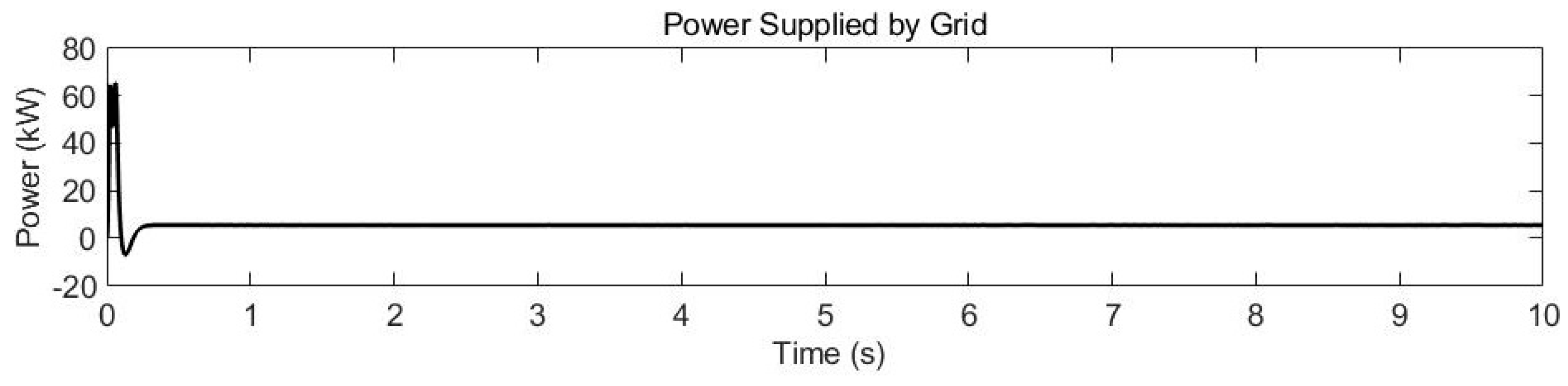
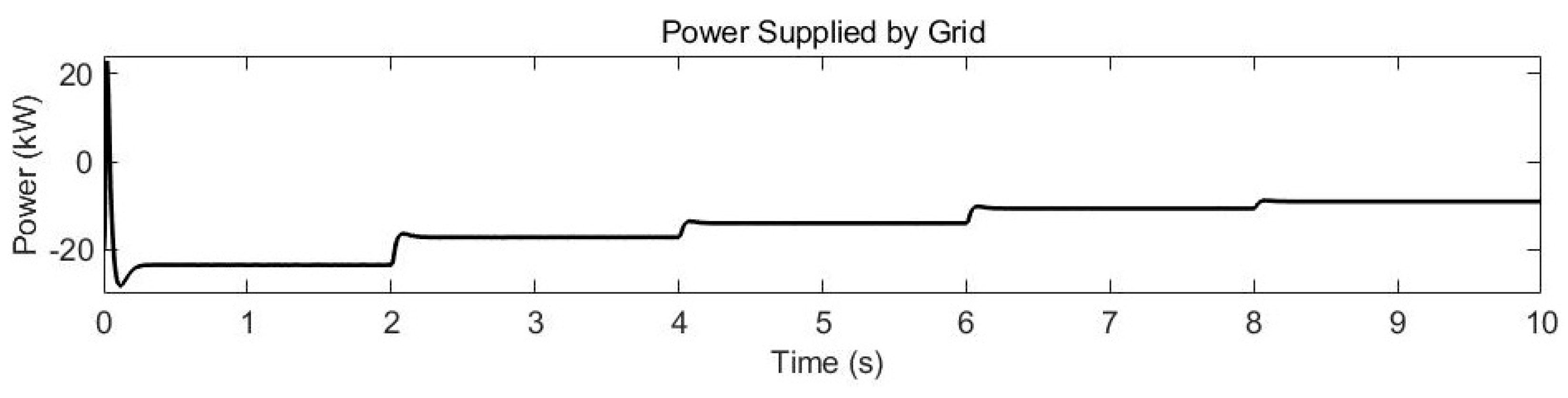
As the simulation progressed, at t = 8 s, solar irradiance further decreased to 100 W/m², reducing the solar PV output to just 4.8 kW. At this point, the system requires significant grid support, as both the BESS and solar PV system can only supply a total of 14.8 kW. The grid must provide the remaining 25.2 kW to meet the 40 kW load demand, as shown in Figure 47. This shift highlights the critical role of grid support during periods of low renewable energy generation, ensuring continuous power supply despite adverse weather conditions.

Figure 47. Power supplied by the grid to the load in nano-grid system.

3.2.3. Test Condition 3: Operation on a Sunny Day

In this test scenario, the simulation model, as shown in Figure 48, was used to evaluate the nano-grid’s performance when solar irradiance is high, and the load demand is low. The AC load was set to 20 kW, as shown in Figure 49, while the solar PV system generated 40 kW of power, as shown in Figure 50. This creates a situation where solar generation exceeds the load demand, and the nano-grid must manage the excess power.

Figure 48. Simulation model to demonstrate a sunny-day operation.

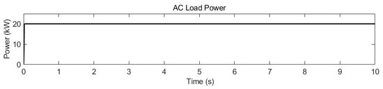
Figure 49. Load demand estimation of AC loads in nano-grid system (Test Condition 3).

Figure 50. Solar PV power generated in nano-grid system.

The system handles this surplus by first directing excess energy towards charging the BESS. The SOC increases beyond 45%, indicating that the battery is being charged, as shown in Figure 51. The battery charges at a steady rate of 5 kW, as shown in Figure 52, ensuring that the system makes efficient use of the available excess solar energy. The remaining surplus power, after meeting both the load demand and battery charging needs, is exported to the grid. This export of power, 15 kW, is shown in Figure 53.

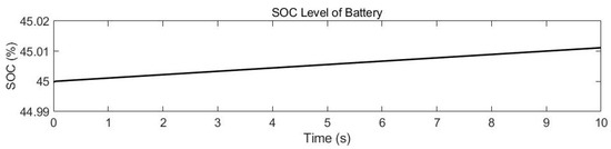
Figure 51. SOC of battery during charging in nano-grid system (Test Condition 3).

Figure 52. Battery capacity of BESS during charging in nano-grid system (Test Condition 3).

Figure 53. Surplus power delivered to the grid in nano-grid system (Test Condition 3).

This simulation highlights the system’s ability to dynamically adjust the power flow to balance solar generation with load demand. With solar generation producing 40 kW and the AC load set at 20 kW, the system efficiently manages the excess energy by charging the battery and exporting the remaining power to the grid. This dynamic adjustment optimizes the use of renewable energy, reducing reliance on external power sources and contributing to overall grid stability.

The gradual increase in the battery’s SOC, as observed in Figure 54, indicates that the charging process is stable and well-controlled. The battery charges at a rate of 5 kW, ensuring that it does not experience any abrupt increases in voltage that could lead to inefficiencies or potential damage. The system’s control algorithms are designed to keep the charging process within safe and optimal parameters, thereby preserving the battery’s health and prolonging its lifespan.

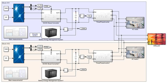
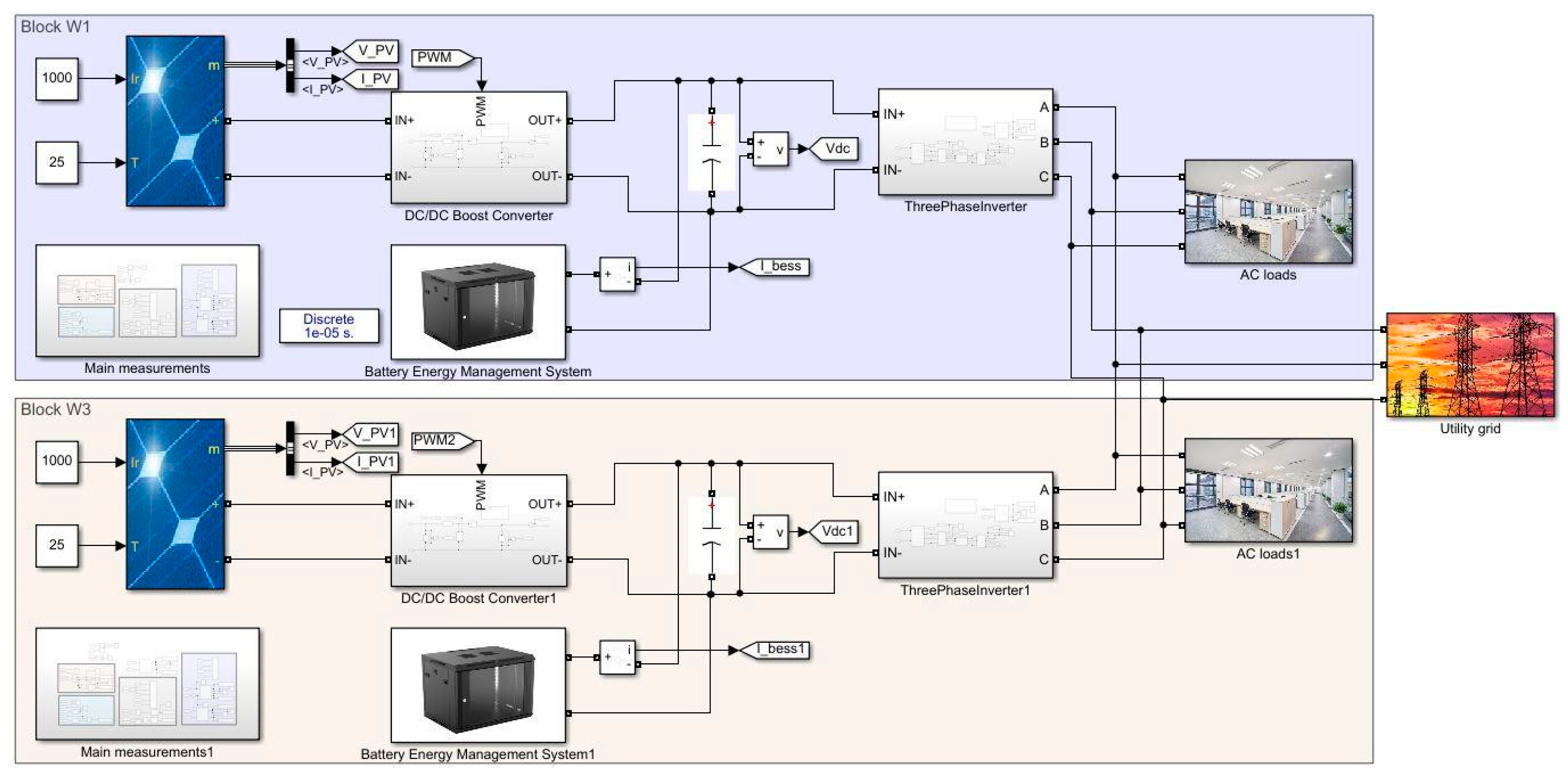
Figure 54. Two parallel nano-grids connected to the three-phase grid.

3.2.4. Test Condition 4: Power Sharing Between Two Nano-Grid Systems

In this test scenario, the simulation model shown in Figure 54 was used to examine the dynamics of the power flow between two buildings, represented by blocks W1 and W3, connected via two parallel nano-grids. These nano-grids are also connected to the utility grid, enabling the system to balance load demands across the buildings. Initially, the AC loads for both buildings were set at 40 kW for the time interval 0 ≤ t < 5 s, as shown in Figure 55. During this period, both blocks have identical load demands, and the system remains balanced, with each nano-grid supplying its own load.

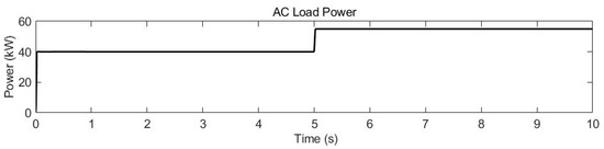
Figure 55. AC loads before an increase for two nano-grids system.

However, at t = 5 s, the load demand in block W3 increases, raising the AC load to 55 kW, while the load in block W1 remains at 40 kW, as shown in Figure 55. Since the solar PV system and BESS in block W3 are insufficient to meet this increased demand, additional power must be drawn from block W1 to support the excess load in block W3. This power transfer between the two nano-grids ensures that the load demand in block W3 is met without compromising the stability of the system.

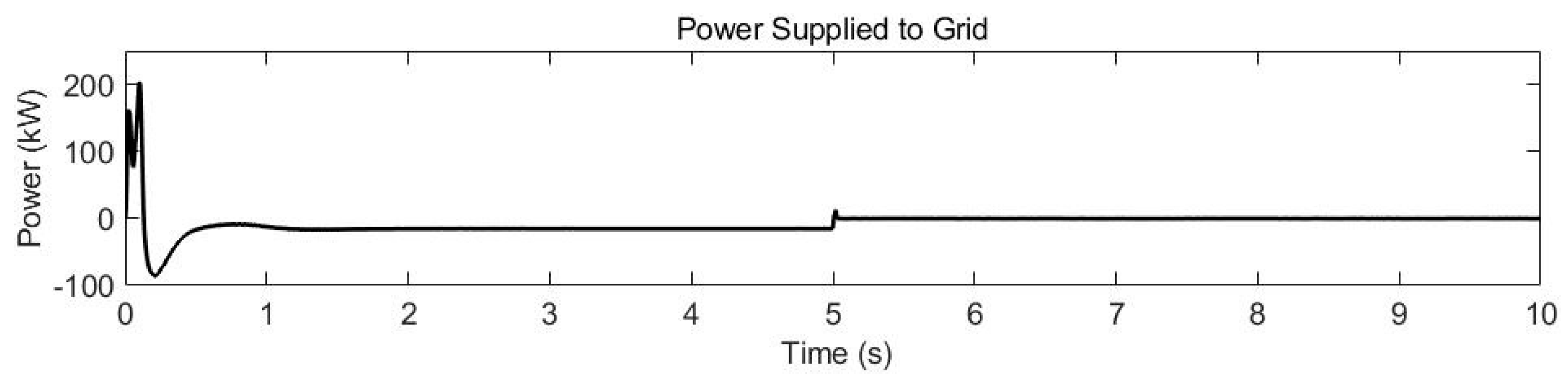
As a result of this increased demand, the surplus power initially being exported to the grid decreases after t = 5 s, as shown in Figure 56. Prior to the increase in load demand, both blocks were generating surplus power, which was exported to the grid. However, after the load increase in block W3, the system prioritizes local demand, reducing the amount of power available for grid export.

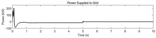
Figure 56. Surplus power from the system sent to the grid for a two-nano-grid system.

4. Conclusions

This study provides a detailed analysis of the operational behavior of pico- and nano-grids during transitions between grid-connected and islanded modes. The simulations that are modelled are based on the SIT campus microgrid and demonstrate the ability of these smaller grids to manage energy flows efficiently and maintain stability under various operational scenarios. This study includes a comprehensive examination of the architectures, subsystem modelling, control algorithms, and operational characteristics of both models, with simulations conducted to understand the power flow, system functionality, and reliability.

In the pico-grid simulations, various scenarios were explored, including battery discharge to loads, nighttime charging, and the parallel operation of two pico-grids to assess load sharing. The pico-grid system proved effective for applications with lower load demands, relying heavily on battery storage and supplemental grid power. When the battery’s state of charge (SOC) is low, support from the grid becomes essential. A parallel operation of multiple pico-grids demonstrated the potential for mutual support and reduced reliance on the grid.

For the nano-grid simulations, scenarios such as solar PV and battery power supply, nighttime battery charging, combined battery and grid power during periods of low solar generation, and the parallel operation of two nano-grids were investigated. The nano-grid system is well-suited for higher load demands due to its integration of solar PV generation and battery storage. However, the variability in solar PV outputs, which is affected by weather conditions, requires additional support from both the battery and the grid. Connecting multiple nano-grids in parallel enhances system reliability and further reduces grid dependency.

The simulation results clearly show how both pico- and nano-grids manage energy flows effectively, maintaining stable SOC levels, DC/AC voltages, and seamless power sharing under varying load conditions. Key scenarios, including grid disconnection, renewable energy fluctuations, and parallel grid operations, were validated with simulation data, confirming the reliability and adaptability of the proposed system.

The next phase involves validating the simulation outcomes with a hardware implementation. A small-scale nano-grid system could be set up on a building rooftop using commercially available solar PV panels, battery storage, a DC charge controller, a single-phase inverter, and a load bank. This setup will enable practical power flow analysis, with real-time data collection facilitated by a power quality data logger. As the nano-grid and pico-grid systems in the SIT campus become fully operational, future work will also include comparing simulation results with actual performance data to ensure accuracy and reliability.

References

- Qazi, A.; Hussain, F.; Rahim, N.A.B.D.; Hardaker, G.; Alghazzawi, D.; Shaban, K.; Haruna, K. Towards Sustainable Energy: A Systematic Review of Renewable Energy Sources, Technologies, and Public Opinions. IEEE Access 2019, 7, 63837–63851. [Google Scholar] [CrossRef]
- Pali, B.S.; Vadhera, S. Renewable Energy Systems for Generating Electric Power: A Review. In Proceedings of the 2016 IEEE 1st International Conference on Power Electronics, Intelligent Control and Energy Systems (ICPEICES), Delhi, India, 4–6 July 2016. [Google Scholar]
- Andujar, J.M.; Segura, F.; Dominguez, T. Study of a Renewable Energy Sources-Based Smart Grid: Requirements, Targets, and Solutions. In Proceedings of the 2016 3rd Conference on Power Engineering and Renewable Energy (ICPERE), Yogyakarta, Indonesia, 16–18 September 2016. [Google Scholar]
- Ullah, Z.; Asghar, R.; Khan, I.; Ullah, K.; Waseem, A.; Wahab, F.; Haider, A.; Ali, S.M.; Jan, K.U. Renewable Energy Resources Penetration within Smart Grid: An Overview. In Proceedings of the 2020 International Conference on Electrical, Communication, and Computer Engineering (ICECCE), Istanbul, Turkey, 12–13 June 2020. [Google Scholar]
- El-Shahat, A. Nanogrid Technology Increasing, Supplementing Microgrids. Nat. Gas Electr. 2016, 33, 1–7. [Google Scholar] [CrossRef]
- Burmester, D.; Rayudu, R.; Seah, W.; Akinyele, D. A Review of Nanogrid Topologies and Technologies. Renew. Sustain. Energy Rev. 2017, 67, 760–775. [Google Scholar] [CrossRef]
- Rai, S.K.; Mathur, H.D.; Bansal, R.C. Optimal energy management of nanogrid using battery storage system. Sustain. Energy Technol. Assess. 2023, 55, 102921. [Google Scholar] [CrossRef]
- Nordman, B.; Christensen, K. Local power distribution with nanogrids. In Proceedings of the 2013 International Green Computing Conference Proceedings, Arlington, VA, USA, 27–29 June 2013; pp. 1–8. [Google Scholar]
- Werth, A.; Kitamura, N.; Tanaka, K. Conceptual Study for Open Energy Systems: Distributed Energy Network Using Interconnected DC Nanogrids. IEEE Trans. Smart Grid 2015, 6, 1621–1630. [Google Scholar] [CrossRef]
- Jirdehi, M.A.; Ahmadi, S. The optimal energy management in multiple grids: Impact of interconnections between microgrid–nanogrid on the proposed planning by considering the uncertainty of clean energies. ISA Trans. 2022, 131, 323–338. [Google Scholar] [CrossRef] [PubMed]
- de Oliveira, F.M.; Mariano, A.C.S.; Salvadori, F.; Ando Junior, O.H. Power Management and Power Quality System Applied in a Single-Phase Nanogrid. Energies 2022, 15, 7121. [Google Scholar] [CrossRef]
- Sulthan, S.M.; Siddhara, S.A.; Revathi, S.B.; Mansoor, O.M.; Veena, R.; Ahamed, T.P.I. Centralized power management and control of a low voltage DC nanogrid. Energy Rep. 2023, 9 (Suppl. 10), 1513–1520. [Google Scholar] [CrossRef]
- Joos, G.; Agbossou, B.L.; Ould-Ben-Tahar, T. Real-time control and energy management system for a hybrid AC/DC nanogrid. IEEE Trans. Sustain. Energy 2022, 13, 2038–2048. [Google Scholar]
- Kumar, P.; Maurya, V.N.; Shukla, S. Adaptive hierarchical control strategy for energy management in a nanogrid using fuzzy logic. IEEE Trans. Ind. Appl. 2020, 56, 4321–4332. [Google Scholar]
- Yu, X.; Xue, Y.; Guerrero, J.L.; Gadh, R. An event-triggered droop control method for dynamic power sharing in nanogrid clusters. IEEE Trans. Power Electron. 2017, 32, 7951–7961. [Google Scholar]
- Hussain, A.; Bui, V.H.; Kim, H.M. Microgrids as a Resilience Resource and Strategies Used by Microgrids for Grid Support: A Comprehensive Review. IEEE Access 2019, 7, 123744–123764. [Google Scholar]
- Bagherzadeh, L.; Shahinzadeh, H.; Shayeghi, H.; Dejamkhooy, A.; Bayindir, R.; Iranpour, M. Integration of Cloud Computing and IoT (CloudIoT) in Smart Grids: Benefits, Challenges, and Solutions. In Proceedings of the 2020 International Conference on Computational Intelligence for Smart Power System and Sustainable Energy (CISPSSE), Keonjhar, India, 29–31 July 2020; pp. 1–8. [Google Scholar]
- Shahinzadeh, H.; Mirhedayati, A.-S.; Shaneh, M.; Nafisi, H.; Gharehpetian, G.B.; Moradi, J. Role of Joint 5G-IoT Framework for Smart Grid Interoperability Enhancement. In Proceedings of the 2020 15th International Conference on Protection and Automation of Power Systems (IPAPS), Shiraz, Iran, 30–31 December 2020; pp. 12–18. [Google Scholar]
- Ullah, H.; Siddiqui, A.S.; Naeem, M.; Alghamdi, A.S. Peer-to-Peer Energy Trading in Smart Grids: A Comprehensive Review. IEEE Access 2021, 9, 43444–43462. [Google Scholar]
- Pop, C.; Cioara, T.; Antal, M.; Anghel, I.; Salomie, I.; Bertoncini, M. Blockchain Based Decentralized Management of Demand Response Programs in Smart Energy Grids. Sensors 2018, 18, 162. [Google Scholar] [CrossRef] [PubMed]
- Qayyum, F.; Jamil, H.; Jamil, F.; Kim, D. Predictive Optimization Based Energy Cost Minimization and Energy Sharing Mechanism for Peer-to-Peer Nanogrid Network. IEEE Access 2022, 10, 23593–23604. [Google Scholar] [CrossRef]
- Morstyn, T.; Farrell, N.; Darby, S.J.; McCulloch, M.D. Using peer-to-peer energy-trading platforms to incentivize prosumers to form federated power plants. Nat. Energy 2018, 3, 94–101. [Google Scholar] [CrossRef]
- Fortuna, L.; Arturo, B. Sustainable Energy Systems. Energies 2022, 15, 9227. [Google Scholar] [CrossRef]
- Singapore Institute of Technology. A Smart Campus to Call Home—SIT Begins Construction of Centralised Campus in Punggol with Groundbreaking Ceremony. 27 April 2021. Available online: https://www.singaporetech.edu.sg/digitalnewsroom/a-smart-campus-to-call-home--sit-begins-construction-of-centralised-campus-in-punggol-with-groundbreaking-ceremony/ (accessed on 1 June 2024).
- Enterprise Singapore. Code of Practice for Energy Efficiency Standard for Building Services and Equipment; Springer: Singapore, 2014. [Google Scholar]
- Building and Construction Authority (BCA). GM ENRB: 2017—Green Mark for Non-Residential Buildings. Available online: https://www1.bca.gov.sg/docs/default-source/docs-corp-buildsg/sustainability/green-mark-enrb-2017-technical-guide_(11feb2020)-to-upload708672f9aeaf4cb58ceb01298bd1de70.pdf (accessed on 1 June 2024).
- Rashid, M.H. Power Electronics: Circuits, Devices & Applications; Pearson: London, UK, 2013. [Google Scholar]
- Wang, W.; Li, J.; Li, H.; Wang, P. Modelling and Control of Bidirectional DC-DC Converter in Energy Storage Applications. In Proceedings of the 2013 IEEE Energy Conversion Congress and Exposition (ECCE), Denver, CO, USA, 15–19 September 2013; pp. 1024–1031. [Google Scholar] [CrossRef]
- Erickson, R.W.; Maksimovic, D. Fundamentals of Power Electronics, 2nd ed.; Kluwer Academic Publishers: Norwell, MA, USA, 2001. [Google Scholar]
- Bhaskar, M.; Ashok, S. PV-Fed Bidirectional DC-DC Converter for Battery Management System. In Proceedings of the 2015 IEEE International Conference on Power Electronics, Drives and Energy Systems (PEDES), Bangalore, India, 16–19 December 2015; pp. 1–6. [Google Scholar]
- Esram, T.; Chapman, P.L. Comparison of Photovoltaic Array Maximum Power Point Tracking Techniques. IEEE Trans. Energy Convers. 2007, 22, 439–449. [Google Scholar] [CrossRef]
Disclaimer/Publisher’s Note: The statements, opinions and data contained in all publications are solely those of the individual author(s) and contributor(s) and not of MDPI and/or the editor(s). MDPI and/or the editor(s) disclaim responsibility for any injury to people or property resulting from any ideas, methods, instructions or products referred to in the content. |
© 2024 by the authors. Licensee MDPI, Basel, Switzerland. This article is an open access article distributed under the terms and conditions of the Creative Commons Attribution (CC BY) license (https://creativecommons.org/licenses/by/4.0/).