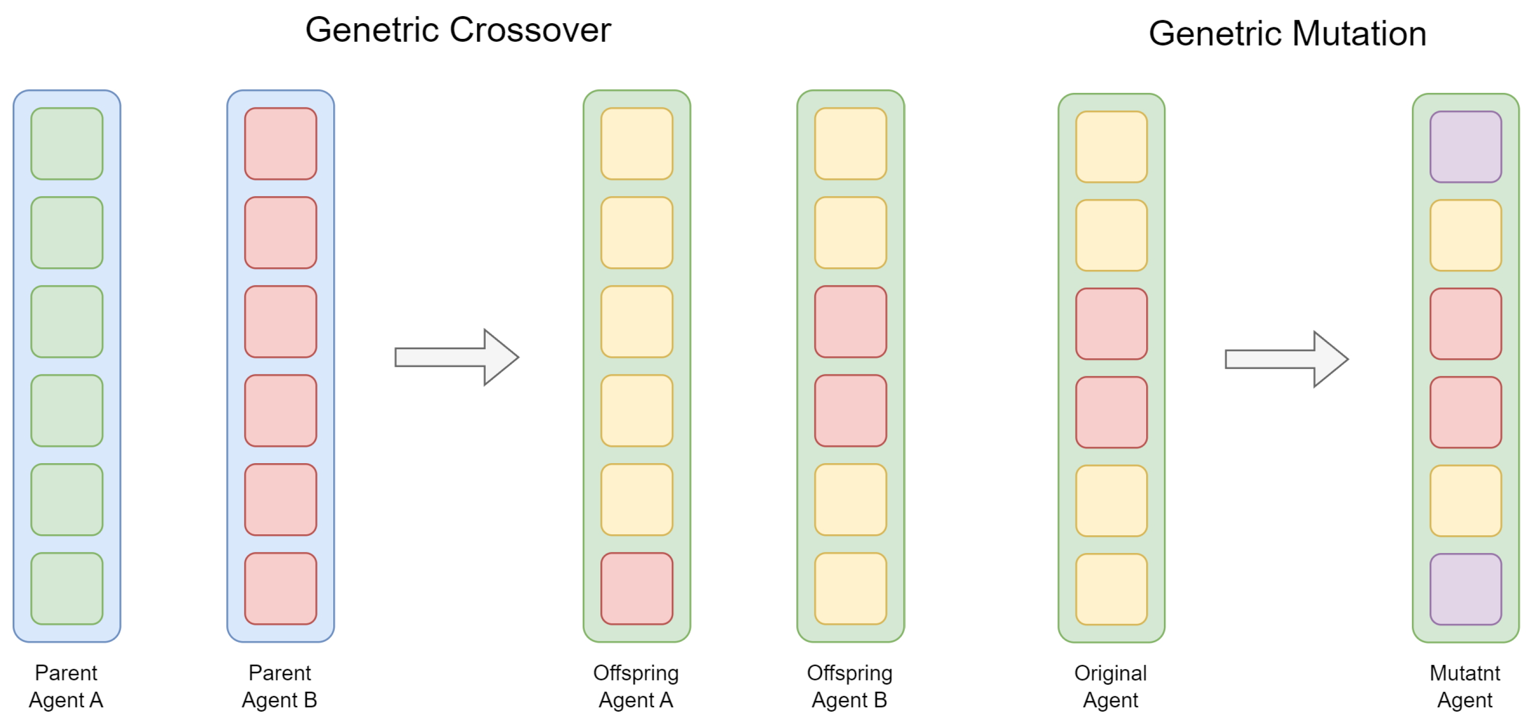
You are currently viewing a new version of our website. To view the old version click .
Energies
  • Article
  • Open Access

30 December 2024

Optimizing Lightweight Recurrent Networks for Solar Forecasting in TinyML: Modified Metaheuristics and Legal Implications

,
,
,
,
and
1
Kosovo and Metohija Academy of Applied Studies, Dositeja Obradovića BB, 38218 Leposavic, Serbia
2
Faculty of Tourism and Hospitality Management, Singidunum University, Danijelova 32, 11000 Belgrade, Serbia
3
Faculty of Informatics and Computing Singidunum University, Danijelova 32, 11000 Belgrade, Serbia
4
Faculty of Informatics and Computer Science, University of Union-Nikola Tesla, 11000 Belgrade, Serbia
This article belongs to the Special Issue Tiny Machine Learning for Energy Applications

Abstract

The limited nature of fossil resources and their unsustainable characteristics have led to increased interest in renewable sources. However, significant work remains to be carried out to fully integrate these systems into existing power distribution networks, both technically and legally. While reliability holds great potential for improving energy production sustainability, the dependence of solar energy production plants on weather conditions can complicate the realization of consistent production without incurring high storage costs. Therefore, the accurate prediction of solar power production is vital for efficient grid management and energy trading. Machine learning models have emerged as a prospective solution, as they are able to handle immense datasets and model complex patterns within the data. This work explores the use of metaheuristic optimization techniques for optimizing recurrent forecasting models to predict power production from solar substations. Additionally, a modified metaheuristic optimizer is introduced to meet the demanding requirements of optimization. Simulations, along with a rigid comparative analysis with other contemporary metaheuristics, are also conducted on a real-world dataset, with the best models achieving a mean squared error (MSE) of just 0.000935 volts and 0.007011 volts on the two datasets, suggesting viability for real-world usage. The best-performing models are further examined for their applicability in embedded tiny machine learning (TinyML) applications. The discussion provided in this manuscript also includes the legal framework for renewable energy forecasting, its integration, and the policy implications of establishing a decentralized and cost-effective forecasting system.

1. Introduction

In recent years, the use of fossil fuels has fallen out of favor for power production. The limited nature of fossil resources, as well as their unsustainable characteristics, has led to increased interest in renewable sources [1]. Nevertheless, the integration of renewable sources is not without challenges [2]. Sources such as wind turbines, solar cells, or electric dams can require a comparatively large upfront investment. Additionally, certain sources, such as solar and wind, rely heavily on external factors like the weather, making them unreliable for certain critical applications [3,4]. Despite these challenges, the integration of renewable sources is essential for sustainability and energy independence. The accurate prediction of solar power generation is crucial for efficient grid management and energy trading. Renewable sources also benefit from being relatively clean and decentralized, which can alleviate many losses caused by power line inefficiencies.
The legal framework for the production and distribution of solar power in Western Balkan countries is increasingly harmonized with European Union (EU) legislation, which issues various legal documents to regulate the development of the energy sector and support the use of renewable energy sources. In policies and directives such as the White and Green Papers on energy policy and renewable energy sources, the EU focuses on supply security, environmental protection, and industry competitiveness. Directive 2018/2001/EU [5] highlights the importance of renewable energy use and sets targets for 2030, including reducing CO2 emissions by 40%, increasing the share of renewable energy to 32%, and raising the share of renewables in transportation to 14%. To achieve these goals, member states develop national action plans with strategies, legislative frameworks, and incentives. Since the introduction of this directive, the share of renewable energy in the EU’s energy consumption has grown from 12.5% in 2010 to 23% in 2022 [6].
In line with EU policies, the legal framework for solar energy production and distribution in Western Balkan countries is oriented toward alignment with EU requirements. Although there are differences in the legislation of each country, most apply common standards through laws such as the Energy Act and the Renewable Energy Act, as well as through national energy development strategies. All Western Balkan countries have a basic Energy Act that encompasses renewable energy sources (RESs). This law typically defines the rights and obligations of solar energy producers, the obligation of transmission systems to facilitate grid connections for RES producers, procedures for issuing permits for the construction and commissioning of solar power plants, and incentives for investments in RES through subsidies, feed-in tariffs, or favorable loans.
The use of artificial intelligence (AI) has demonstrated impressive capabilities for handling time-series forecasting [7], even in the energy sector. By leveraging the forecasting abilities of AI algorithms to balance production and demand, better utilization of this valuable resource can be attained. Furthermore, by providing a more accurate and reliable estimate of production, better integration can be achieved with existing power distribution systems, reducing transmission losses [8,9].
However, AI algorithms are often computationally demanding, requiring substantial investments to train and execute predictions. Models are usually run on relatively expensive graphics processing units (GPUs) and require supporting system infrastructure. This can lead to relatively high power demands. Optimized models could potentially be compared and executed on significantly cheaper systems, enabling accurate models to run at a fraction of the hardware costs and with significantly lower power demands. Tiny machine learning (TinyML) [10] is a subset of machine learning (ML) that explores the deployment of ML models on microcontroller units (MCUs). Such deployment could significantly reduce the cost of using ML in deployment, especially in remote locations where solar and wind turbines may be installed. Further use of predictive models could help better integrate forecasting models into Internet of Things (IoT) networks [11,12].
This work explores the use of metaheuristic optimization algorithms to select optimal hyperparameters for three types of recurrent neural networks (RNNs) [13]. The goal is to select lightweight architectures that can be ported to MCUs for field use while maintaining suitable performance. As the task of hyperparameter tuning is often considered NP-hard [14], a modified metaheuristic optimizer is proposed, and a comparative analysis is conducted against several contemporary optimizers on two publicly available datasets, resulting in six experiments in total. The best-performing models are further explored for their forecasting potential once deployed on an MCU. The contributions of this work can be summarized as follows:
  • An exploration of the legal foundations of energy forecasting in the Western Balkan region;
  • The proposal of a lightweight framework for the in situ forecasting of solar energy production using models optimized for MCUs;
  • The introduction of a modified metaheuristic optimizer tailored to the optimization needs of this study;
  • The selection of lightweight time-series forecasting architectures with suitable accuracy for power systems;
  • The implementation of the proposed model on an MCU to evaluate the practical effectiveness of the approach.
The structure of the remaining work is outlined as follows: Section 2 covers preceding works that inspire and support this study. In Section 3, the methodology is discussed in detail. Section 4 and Section 5 discuss the experimental configuration and present the attained results. Section 6 concludes the work and presents proposals for future research in the field.

3. Methodology

3.1. The Variable Neighborhood Search Optimizer

The variable neighborhood search (VNS) [49] algorithm utilizes a systemic approach to adapt the neighborhood structure during optimization. The idea behind this approach is to focus on exploring more distant locations within the search space and allow the algorithm to avoid local and focus on global optima. The main stages of the optimization strategy are shaking, local search, and neighborhood change.
During shaking procedures, a solution in a simulated neighborhood, different from the current best, is selected. The structure of this neighborhood is then meticulously altered to effectively explore regions. This can be represented as
x N k ( x )
where N k ( x ) denotes a neighborhood index in a given iteration K, while x denotes the current solution and x is the output. Once x is determined, a local search is conducted, as described in the following:
f ( x ) f ( x )
If the local search finds an improved solution, meaning f ( x ) < f ( x ) , the current solution is updated to x = x , and the neighborhood index is reset to k = 1 . If not, the algorithm explores more distant neighborhoods by increasing k:
k k + 1
These procedures are repeated until a suitable solution is found or another criterion is met. The VNS algorithm is fairly flexible, and different criteria can be used depending on the goal of optimization.

3.2. The Modified VNS Algorithm

While the original VNS [49] optimizer still showcases admirable performance, extensive testing using congress of evolutionary computing (CEC) benchmarking functions [50] hints that room for improvement exists. Empirical tests also suggest that population diversity improvements can help bolster the outcomes attained by the optimizer. Integrating an adaptive approach could help the modified optimizer strike a better balance between intensification and exploration, further benefiting the attained solution.
Diversification control mechanisms have been proposed in the literature [51] centered on the L 1 norm. This metric allows for the consideration of diversity on both the agent and population levels. Given a set of agents p for an n-dimensional problem, the L 1 norm can be computed as follows:
x j ¯ = 1 m i = 1 m x i j
D j p = 1 m i = 1 m x i j x ¯ j
D p = 1 n i = 1 n D j p ,
where x ¯ denotes the mean vector of agent positions across search space dimensions, with D j p denoting an individual diversity vector denoted as the L 1 norm and D p signifying the diversity score of the entire population.
Since greater diversity is preferred in the early stages, diversity is dynamically adjusted throughout optimization. The L 1 norm manages this diversity via a dynamic threshold parameter, D t . If population diversity is found to be inadequate, the worst-performing agents are removed from the population. Diversity is tracked using D t , with an initial diversity value D t 0 calculated as follows:
D t 0 = j = 1 N P ( u b j l b j ) 2 · N P ,
As the algorithm progresses and solutions approach the optimal region, the value of D t should decrease from the initial value D t = D t 0 according to the following rule:
D t + 1 = D t D t · t T ,
where t and t + 1 represent the current and next iterations, and T is the total number of iterations per run. In the later stages, as D t is gradually reduced, this mechanism will no longer be triggered, regardless of the value of D P .
In each optimization iteration, n r s worst-performing agents are removed from the population, and new solutions are generated using techniques inspired by the GA [31]. If D t < D P , then replacement agents are produced by recombining 2 random agents in the population. If the condition is not met, the two best-performing agents are recombined. By randomly changing the created agent parameters, mutation further alters the obtained solutions. The crossover and mutation mechanisms are depicted in Figure 1.
Figure 1. Genetic crossover and mutation mechanisms.
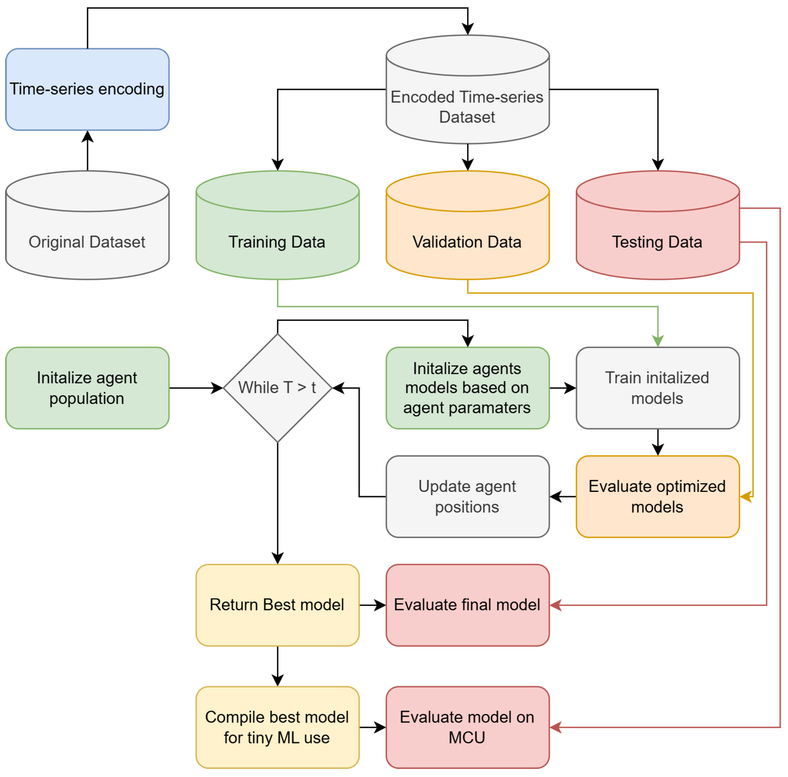
Crossover and mutation are controlled by the crossover and mutational probability parameters C P and M P , which have been shown to provide the best results when set to P C = 0.1 and M P = 0.1 .
The updated metaheuristic incorporates an extra adaptive parameter. To encourage exploration in the early phases of optimization, an adjustable ψ parameter is used. Later phases use the original FA’s [52] remarkably potent intensification plan to encourage exploitation. The following equation presents the search processes for the FA:
X i ( t + 1 ) = X i ( t ) + β e γ r i j 2 ( X j ( t ) X i ( t ) ) + α ϵ i ( t ) ,
where, as of iteration t, r i j indicates the location of agent j, while X i ( t ) represents the position of the firefly. Depending on their distance from one another, the parameter β regulates the attraction between i and j. γ represents the light absorption coefficient, α governs the randomness, and ϵ i ( t ) represents the stochastic vector.
In order to balance exploration and exploitation and enable both algorithms to participate, the ψ parameter is first set to 1.5 and is changed in each iteration in accordance with
ψ t + 1 = ψ t t / T
where t is the current optimization iteration, and T is the total. The FA search will be used if a randomly generated value in the range [ 0 , 1 ] at the beginning of each iteration exceeds ψ ; if not, the VNS search techniques are used. The suggested optimizer is called the diversity-oriented adaptive VNS (DOAVNS) with the included adjustments in mind. Algorithm 1 provides the procedural pseudocode for this optimizer.
Algorithm 1 Proposed DOAVNS optimizer code.
  • Initialize solutions for a population P
  • Set initial states for N R S = 2 , ψ = 1.5
  • while T > t do
  •    for Agent a in P do
  •       Evaluate agent
  •       Assign fitness
  •    end for
  •    Determine D p
  •    Remove worst N R S agents form population
  •    if  D P < D t  then
  •       for  N R S  do
  •          Apply crossover between agents and random agents
  •          Apply mutation to the generated agents
  •       end for
  •    else
  •       for  N R S  do
  •          Apply crossover between the best agent and a random agent
  •          Apply mutation to the generated agents
  •       end for
  •    end if
  •    Select random value R between [ 0 ,   1 ]
  •    if  R > ψ  then
  •       Leverage FA search for updates
  •    else
  •       Leverage VNS search for updates
  •    end if
  • end while
  • return Best attained solution

3.3. The ESP32 Platform for TinyML Use

The ESP32 [53] is a popular platform for IoT devices. The system-on-a-chip offers many advantages with an affordable, small footprint. The device supports several Bluetooth protocols as well as Wi-Fi functionality. In module form, several standard interfaces are available, including UART, I2C, GPIO, DAC, and ADC, as well as SD card support and motor PWM. This makes the ESP32 a very versatile platform for use in IoT networks [54], especially when considering the low minimum current demands of only 500 mA. The module relies on two low-power Xtensa 32-bit LX6 microprocessors and supports 446 KB of ROM as well as 520 KB of on-chip SRAM. The ESP32 can support a real-time operating system (RTOS). A low-power coprocessor can be utilized if computational resources are not required, such as in the case of monitoring peripherals, allowing for further power reduction.
Several frameworks exist for porting ML models for use on the ESP32, with support from the Arduino community [55]. One such framework allows for TensorFlow Lite models to be compiled, loaded, and run on the ESP32. The best-performing model optimized by metaheuristic optimizers in this work is subjected to compilation and adapted for use on the ESP32 chip. The Arduino IDE is used for programming, TensorFlow Lite is used for model compilation, and Python is used to conduct model training and optimization tasks.
TinyML offers considerable cost benefits in hardware and energy consumption. Microcontrollers compatible with TinyML like STM32 and Arduino Nano 33 BLE Sense cost approximately USD 5–20 per unit, compared to traditional IoT or edge devices such as Raspberry Pi or industrial computers, which range from USD 30 to 150. This results in hardware cost savings of up to 80%. In addition, TinyML devices typically consume just 1–10 milliwatts of power, considerably less than the 1–5 watts consumed by standard edge computing devices, resulting in over 90% reduction in energy usage and leading to lower operational costs and reduced battery maintenance needs.
Deployment and maintenance are also more economical with TinyML. These devices require minimal infrastructure and are simpler for management, resulting in an estimated 50% reduction in deployment and maintenance costs in comparison to the standard edge solutions. Furthermore, by processing data on-device, TinyML drastically reduces the volume of data sent to the cloud, considerably lowering bandwidth and storage costs. This can lead to bandwidth savings of up to 70%, which is particularly beneficial in remote or high-data environments.

3.4. Proposed Framework

The framework proposed in this paper includes three-stage optimization. This encompasses data preparation and time-series encoding. A set of samples is used to create a time series, and data are separated into training, testing, and validation portions. Agent populations are generated, and based on solution parameters, models are generated. The generated models are trained using the training portion of the dataset and evaluated on the validation set. Once a termination criterion is met, the final model is evaluated using the withheld training portion. The best trained model is then compiled for use on an MCU, and performance is simulated using the UART input. In other words, once model optimization is completed (typically using more expensive hardware such as GPUs or TPUs), these optimized models can be efficiently deployed on embedded devices, operating with minimal power consumption. A flowchart explaining the proposed framework is presented in Figure 2.
Figure 2. Proposed framework flowchart.
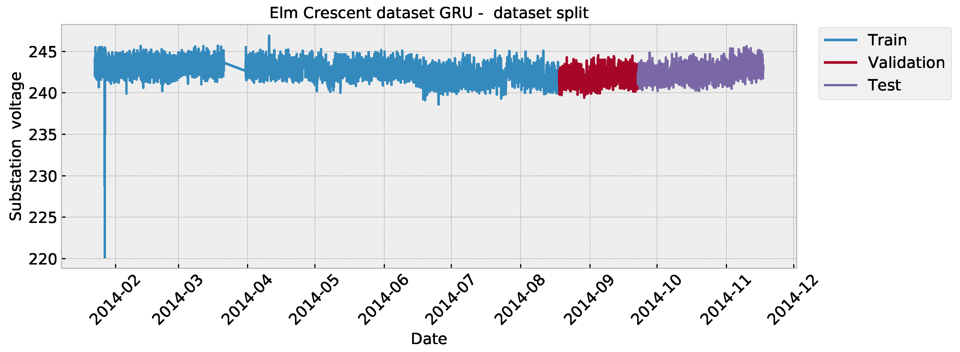
4. Experimental Setup

To evaluate the effectiveness of the proposed method, a publicly available dataset sourced from the real world was used, which can be found on Kaggle (https://www.kaggle.com/datasets/pythonafroz/solar-panel-energy-generation-data, accessed on 25 October 2024). The simulations concentrated on the Elm Crescent and Forest Road segments of the dataset. The data were sequentially divided into training, validation, and testing sets in a 70/10/20 ratio. Simulations were performed with a 12-step lag and 1-step-ahead targets. The dataset divisions are illustrated in Figure 3 for the Elm Crescent and in Figure 4 for the Forest Road portion of the dataset.
Figure 3. Elm Crescent dataset visualization.
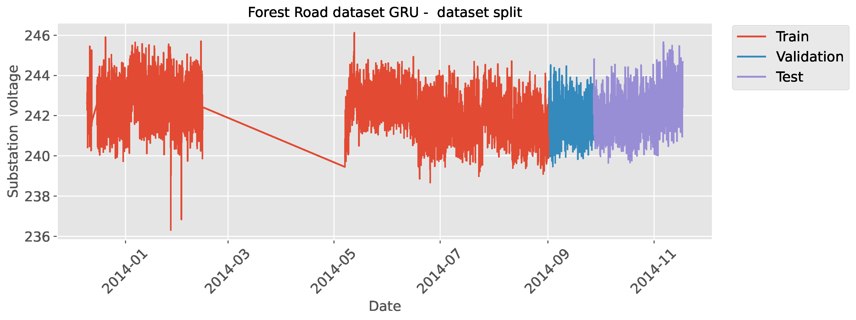
Figure 4. Forest Road dataset visualization.
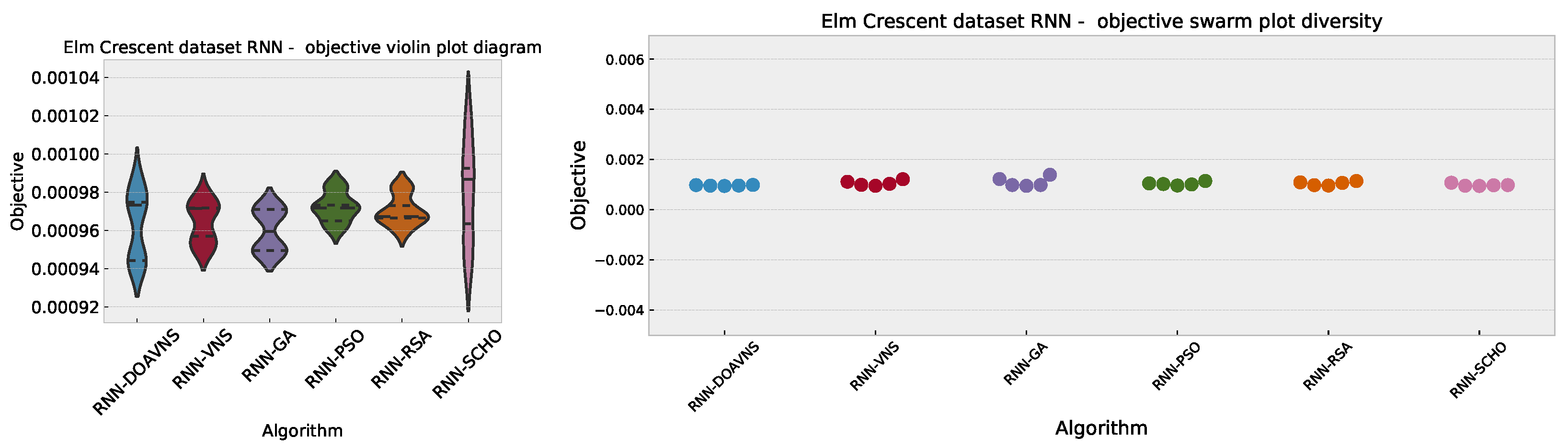
A comparative simulation was conducted between the proposed algorithm and the baseline VNS [49]. The evaluation also included other algorithms, such as the GA [31], PSO [30], RSA [32], and SCHO [33]. Each optimizer was implemented separately for the simulations using the parameter configurations specified in the original papers for each algorithm. Seven iterations were performed for each optimizer, utilizing a population of five individuals, and the simulations were run independently 30 times due to the high computational cost associated with optimization. The optimizers were responsible for hyperparameter selection for the RNN, LSTM, and GRU models using empirically determined ranges, as detailed in Table 1.
Table 1. Parameter ranges for RNN, LSTM, and GRU networks.
Model performance is assessed using standard regression metrics [56].
RMSE = 1 n i = 1 n b i b ^ i 2
MAE = 1 n i = 1 n b i b ^ i
MSE = 1 n i = 1 n ( b i b ^ i ) 2
R 2 = 1 i = 1 n ( b i b ^ i ) 2 i = 1 n ( b i b ¯ ) 2
An additional metric known as the index of agreement (IoA) [57] was also tracked during optimization to provide a more comprehensive view of the models’ performance. The formula for this metric is provided below:
IoA = 1 i = 1 n ( b i b ^ i ) 2 i = 1 n ( | b i b ¯ |   +   | b i b ^ i | ) 2
In the given formulas, b i and b ^ i represent the actual and predicted values for the i-th sample, b ¯ represents the mean value, and n is the sample size. For the simulations performed, MSE is used as the objective function, while R 2 serves as the indicator function.

5. Simulation Outcomes

The simulation outcomes attained in the conducted experiments are presented in three parts. Firstly, the simulation scores of the RNN on the Elm Crescent and Forest Road datasets are presented. In all tables containing simulation outcomes, the best score in every observed category is highlighted in bold. Then, LSTM simulation outcomes are presented in the same order. Finally, simulations with GRU are presented. The best-performing models in each set of simulations are then compared separately in terms of detailed metrics. The outcomes are subjected to statistical validation. Finally, simulations for a model deployed on an ESP32 are reported.

5.1. RNN Simulations

5.1.1. RNN Elm Crescent Simulations

Comparisons in terms of the objective function for Elm Crescent RNN simulation scores are presented in Table 2. The introduced optimizer attained the best-performing model, scoring an objective function result of 0.000943 . The GA showcases impressive performance, achieving the best scores in the worst, mean, and median outcomes, while the PSO showcases the highest rate of stability despite not matching the favorable performance of other optimizers. Further stability comparisons are provided in terms of objective and indicator score distribution diagrams for the objective function in Figure 5 and indicator function in Figure 6. While the modified optimizer showcases a lower rate of stability in comparison to the baseline optimizer, this is to be somewhat expected when boosting algorithm diversification. Furthermore, this drop in stability allowed the optimizer to explore more promising regions of the search space, ultimately attaining the best-performing parameter selections for this test case.
Table 2. Elm Crescent RNN simulations’ objective function outcomes.
Figure 5. Elm Crescent RNN simulations’ objective function distribution diagrams.
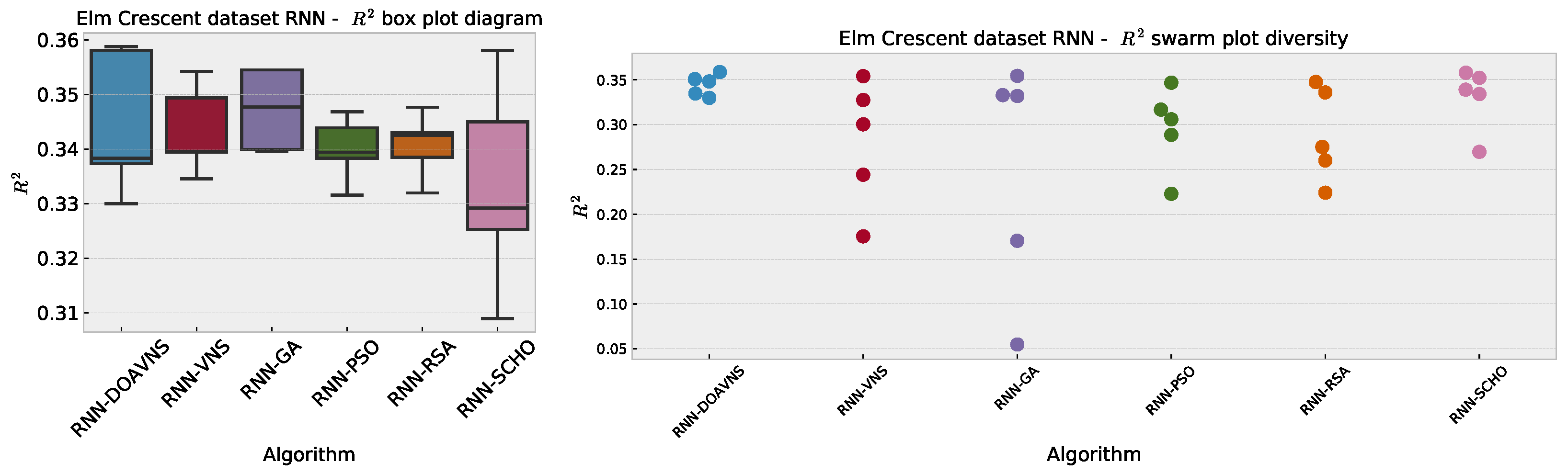
Figure 6. Elm Crescent RNN simulations’ indicator function distribution diagrams.
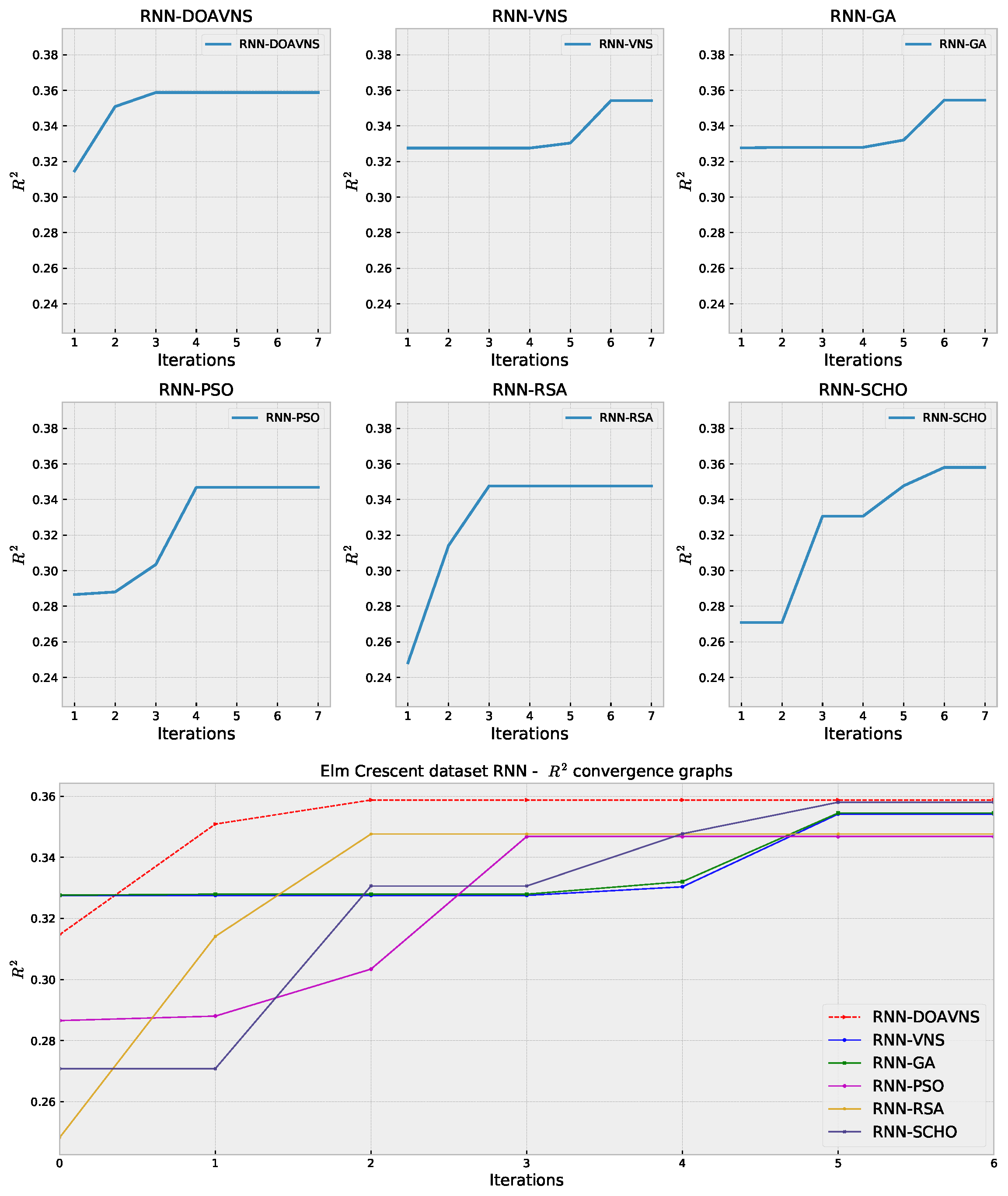
Further comparisons in terms of detailed metrics are provided in Table 3. The model optimized by the introduced DOAVNS optimizer showcases a definitive advantage over other models, attaining the best scores across all metrics.
Table 3. Elm Crescent RNN simulations’ detailed metrics for the best-performing optimized models.
Further insights into the performance of the optimizer and its ability to prevent premature stagnation, as well as avoid being trapped in local optima, are showcased in terms of convergence diagrams. For each of the algorithms included in the comparative analysis, convergence diagrams in terms of objective and indicator functions are provided in Figure 7 and Figure 8. The boost in diversification helps the introduced optimizer converge toward an optimum, while other algorithms struggle with local best solutions.
Figure 7. Elm Crescent RNN simulations’ objective function convergence diagrams.
Figure 8. Elm Crescent RNN simulations’ indicator function convergence diagrams.
The parameter selections made by each algorithm for the respective best-performing model are provided in Table 4 to facilitate simulation repeatability. The predictions made by the best-performing model are provided in Figure 9, while the plot of the error over time is presented in Figure 10.
Table 4. Best-performing RNN model parameter selections for Elm Crescent simulations.
Figure 9. Forecasts of best DOAVNS model from Elm Crescent RNN simulations.
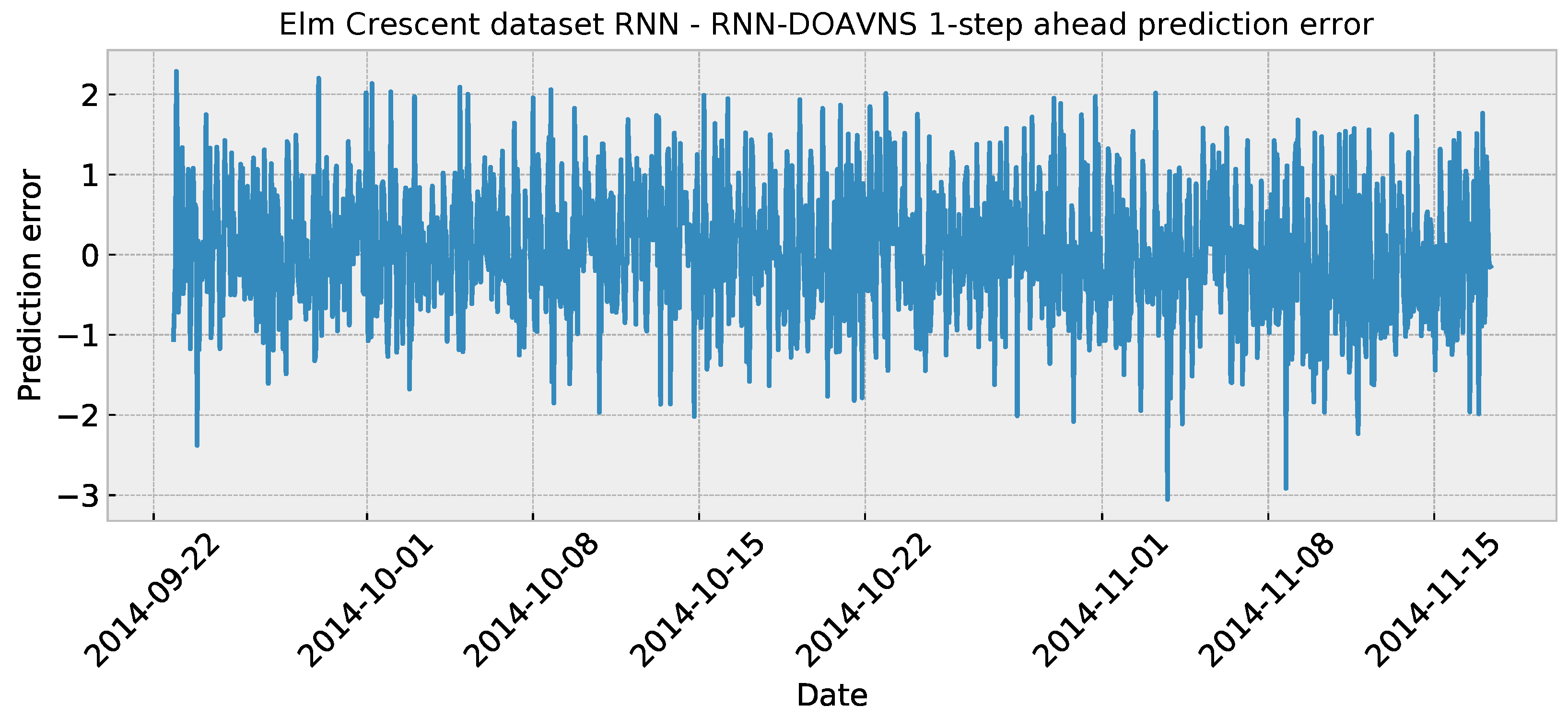
Figure 10. Elm Crescent RNN simulations’ error over time.
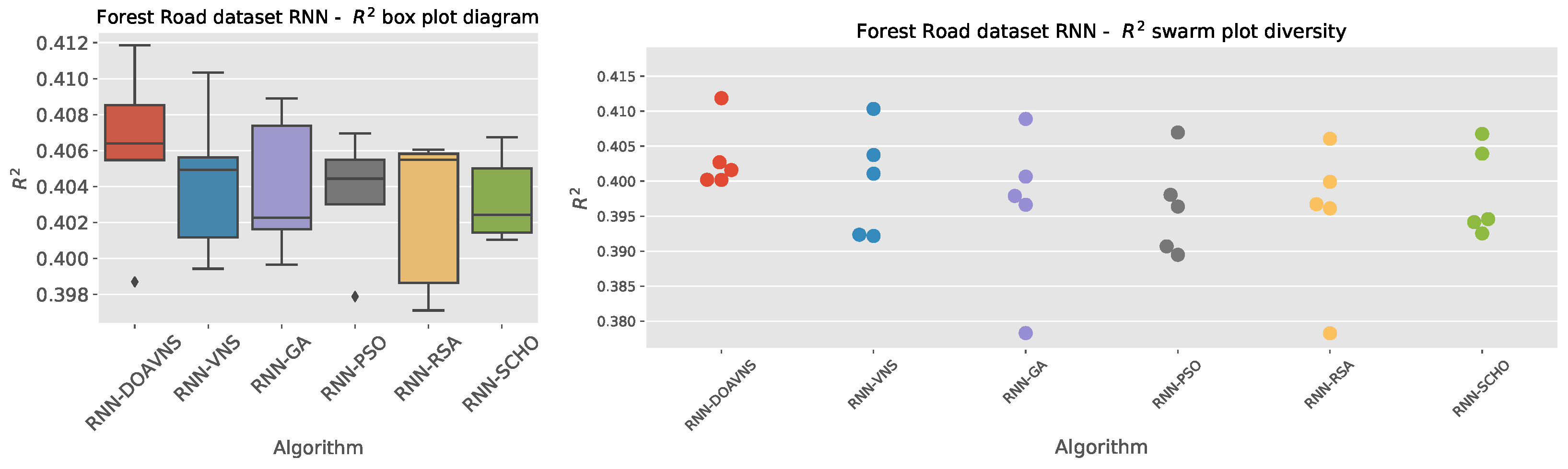
5.1.2. RNN Forest Road Simulations

Comparisons in terms of the objective function for Forest Road RNN simulation scores are presented in Table 5. The introduced optimizer attained the best-performing model, scoring an objective function result of 0.000943 . The introduced optimizer showcases superior performance in the mean and median outcomes, with respective scores of 0.007275 and 0.007275 . The SCHO algorithm attained the best outcomes in terms of worst-case simulations. The highest rate of stability is demonstrated by the SCHO. Further stability comparisons are provided in terms of objective and indicator score distribution diagrams for the objective function in Figure 11 and indicator function in Figure 12. The modified algorithm showcases a slightly reduced stability in this set of simulations, focusing on a more promising region in comparison to all other optimizers, as well as the baseline PSO.
Table 5. Forest Road RNN simulations’ objective function outcomes.
Figure 11. Forest Road RNN simulations’ objective function distribution diagrams.
Figure 12. Forest Road RNN simulations’ indicator function distribution diagrams.
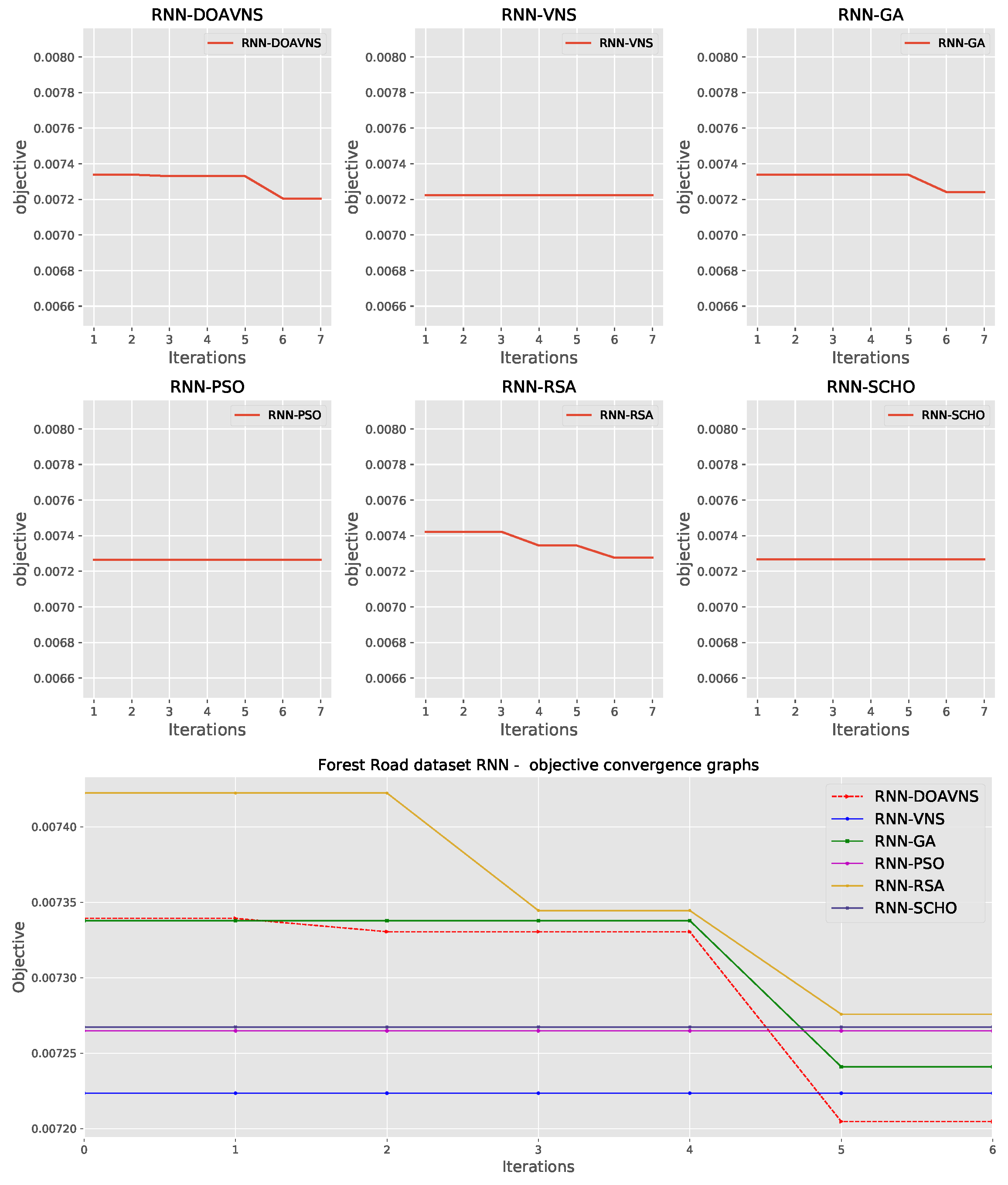
Further comparisons in terms of detailed metrics are provided in Table 6. The model optimized by the introduced DOAVNS optimizer showcases the best scores in terms of R2, MSE, and RMSE, while the GA showcases a high score in terms of MAE, and the SCHO showcases the best IoA score.
Table 6. Forest Road RNN simulations’ detailed metrics for the best-performing optimized models.
Convergence diagrams for each optimizer are provided in Figure 13 and Figure 14 for objective and indicator scores. The introduced optimizer overcomes a local optimum and converges toward a better solution in iteration five, outperforming competing optimizers.
Figure 13. Forest Road RNN simulations’ objective function convergence diagrams.
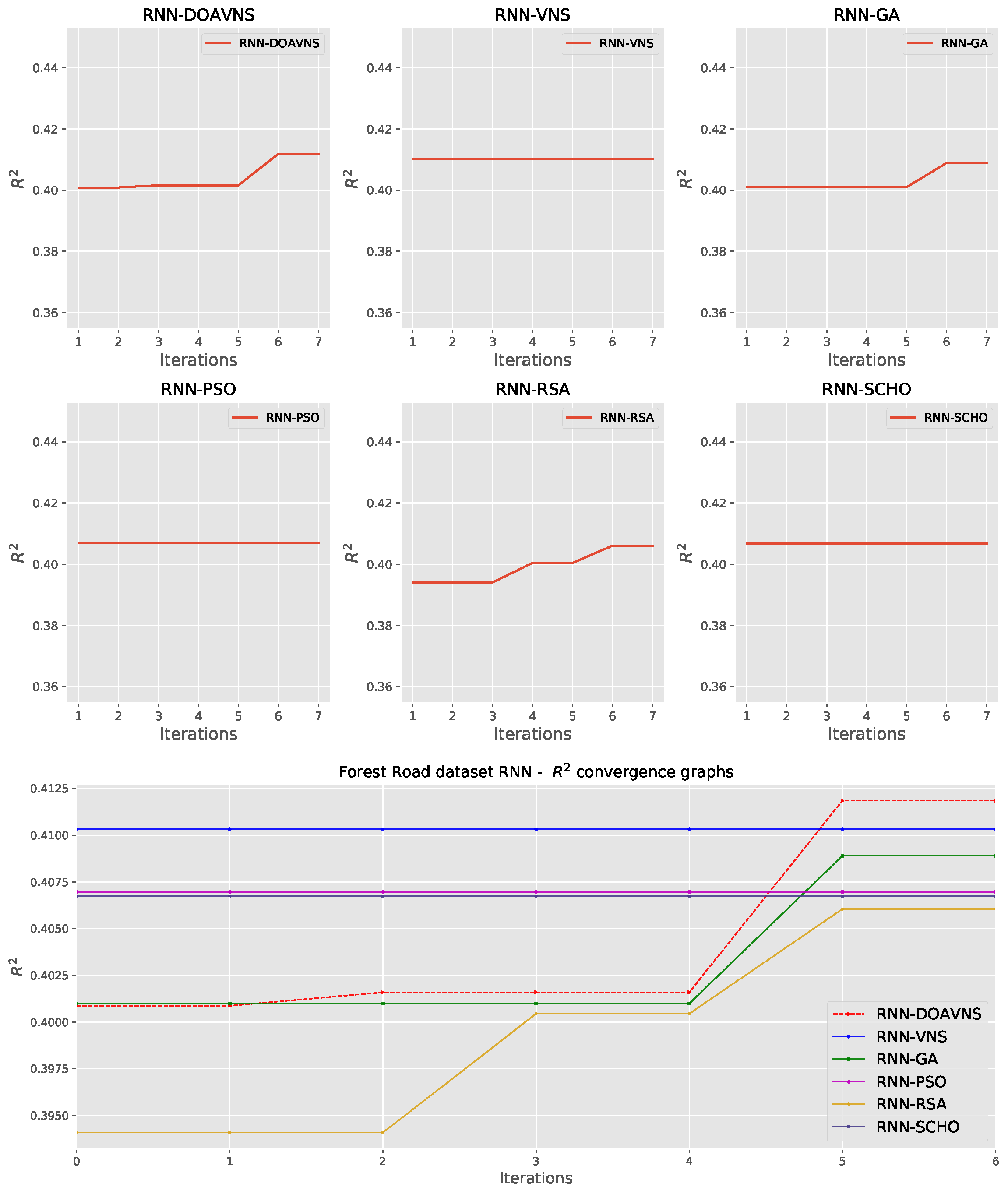
Figure 14. Forest Road RNN simulations’ indicator function convergence diagrams.
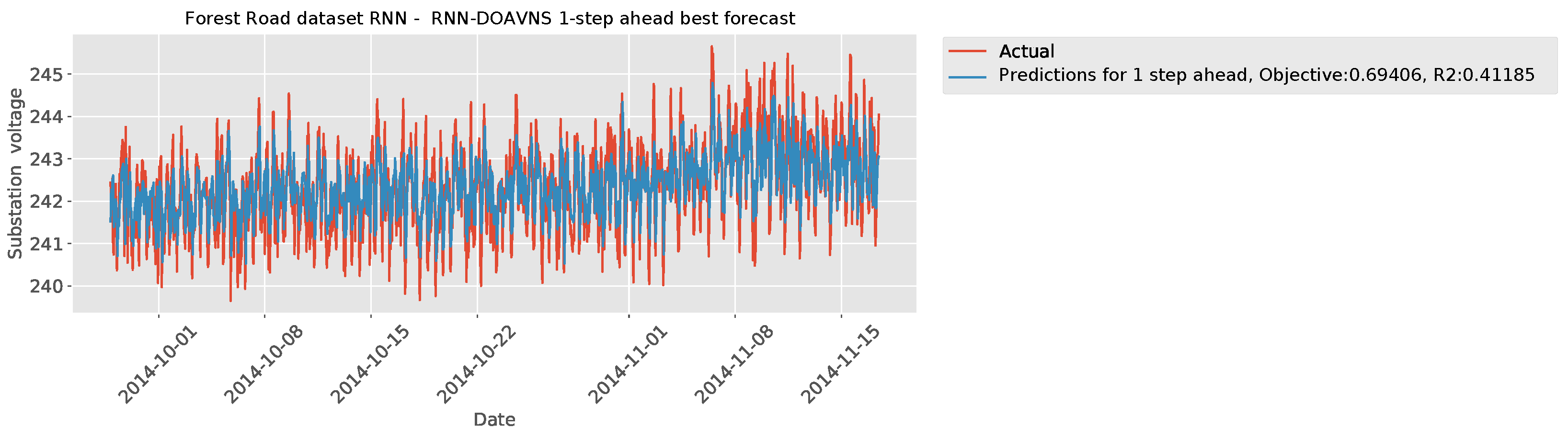
The parameter selections made by each algorithm for the respective best-performing model are provided in Table 7 to facilitate simulation repeatability. The predictions made by the best-performing model are provided in Figure 15, while the plot of the error over time is showcased in Figure 16.
Table 7. Best-performing RNN model parameter selections for Forest Road simulations.
Figure 15. Forecasts of best DOAVNS model from Forest Road RNN simulations.
Figure 16. Forest Road RNN simulations’ error over time.
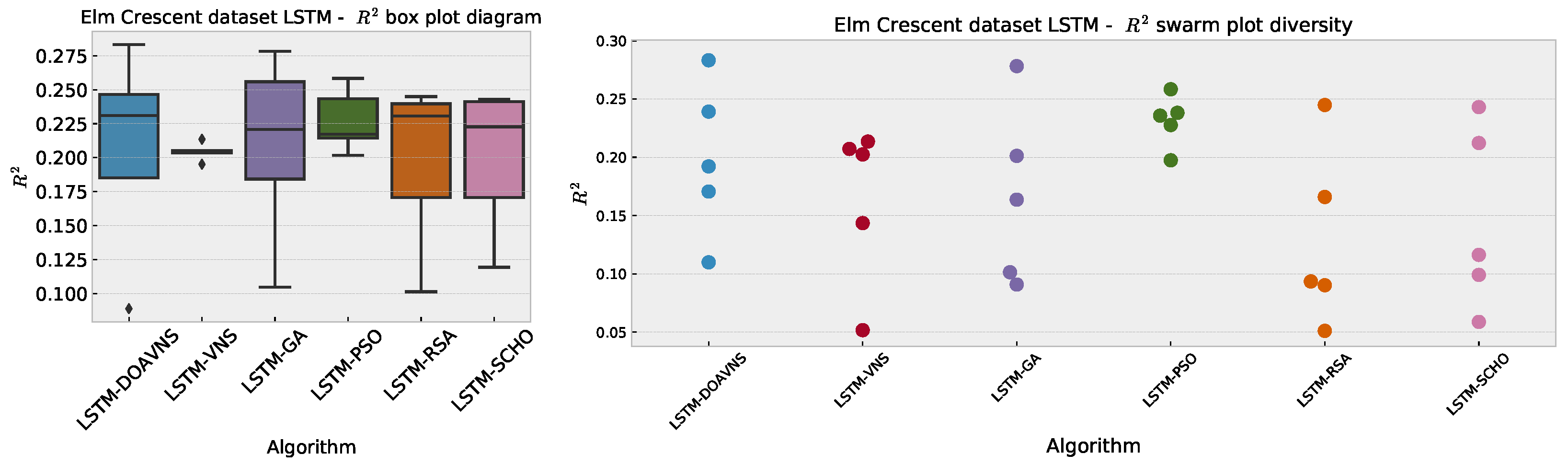
5.2. LSTM Simulations

5.2.1. LSTM Elm Crescent Simulations

Comparisons in terms of the objective function for Elm Crescent LSTM simulation scores are presented in Table 8. The introduced optimizer attained the best-performing model, scoring an objective function result of 0.001054 . The PSO optimizer showcases decent results for the worst and mean scores; however, the introduced optimizer showcases the highest median scores. The VNS showcases the highest rate of stability when compared to other optimizers included in the comparative simulations. Further stability comparisons are provided in terms of objective and indicator score distribution diagrams for the objective function in Figure 17 and indicator function in Figure 18. A notable drop in stability can be observed for the introduced optimizer. This is to be somewhat expected with increasing diversification. However, the introduced modifications help improve performance, allowing the introduced modified algorithm to locate the most promising region and attain the highest objective scores.
Table 8. Elm Crescent LSTM simulations’ objective function outcomes.
Figure 17. Elm Crescent LSTM simulations’ objective function distribution diagrams.
Figure 18. Elm Crescent LSTM simulations’ indicator function distribution diagrams.
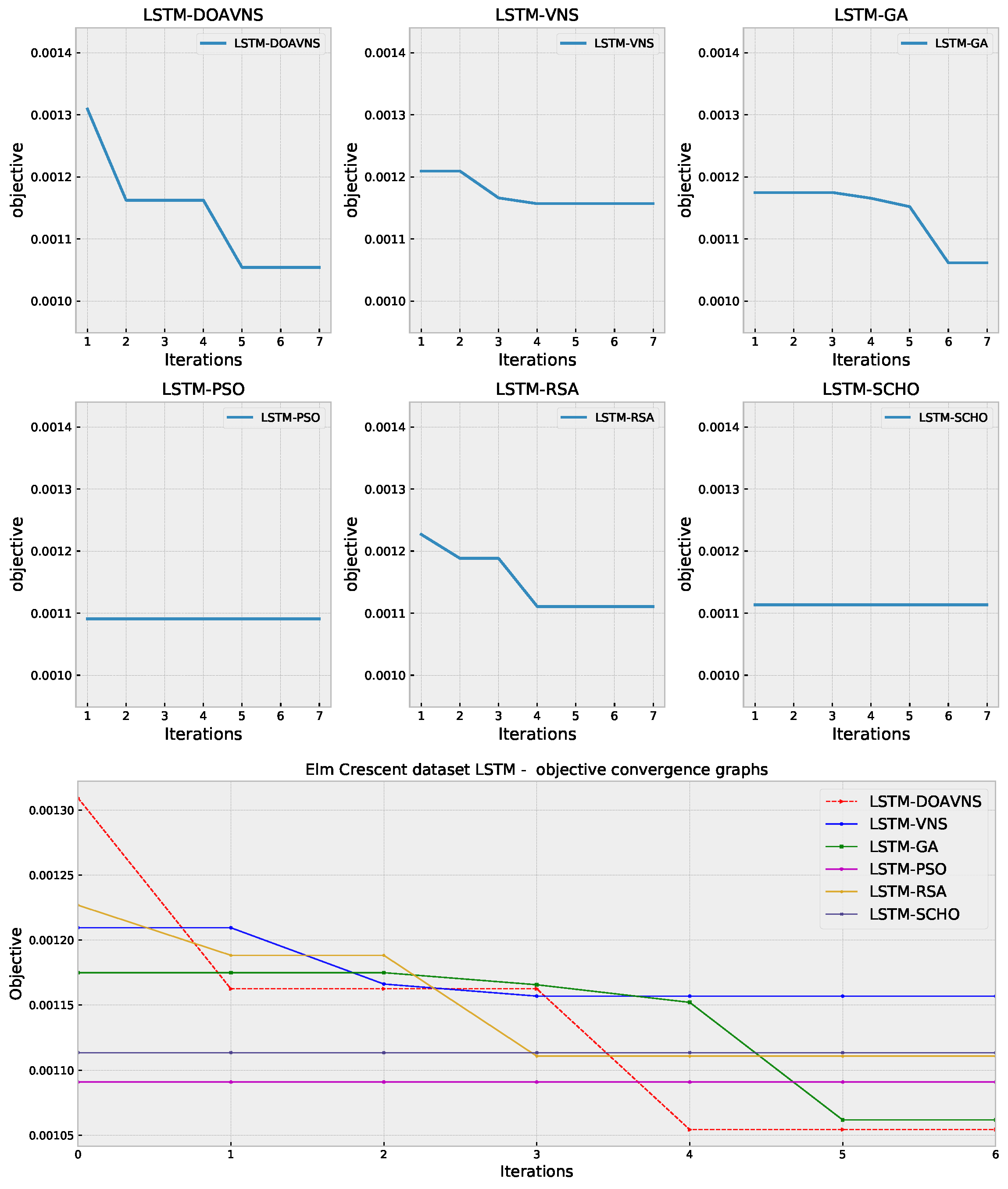
Further comparisons in terms of detailed metrics are provided in Table 9. The model optimized by the introduced DOAVNS optimizer showcases the best scores in terms of all metrics except the IoA, where the GA showcases the highest score.
Table 9. Elm Crescent LSTM simulations’ detailed metrics for the best-performing optimized models.
Convergence diagrams for each optimizer are provided in Figure 19 and Figure 20 for objective and indicator scores. The introduced optimizer overcomes a local optimum and converges toward a better solution in iteration four, outperforming competing optimizers.
Figure 19. Elm Crescent LSTM simulations’ objective function convergence diagrams.
Figure 20. Elm Crescent LSTM simulations’ indicator function convergence diagrams.
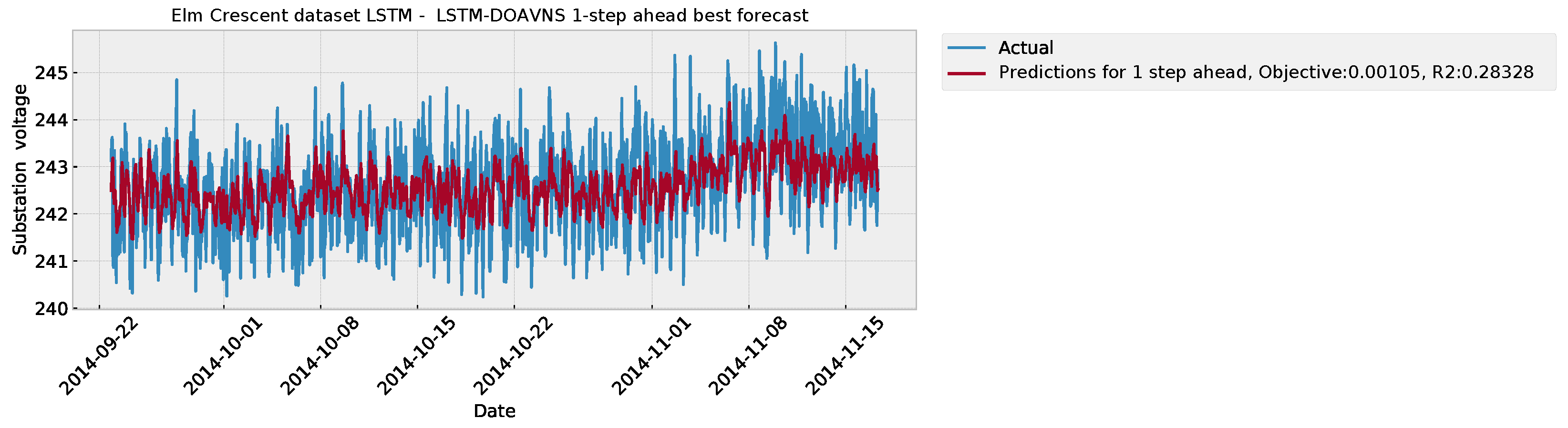
The parameter selections made by each algorithm for the respective best-performing model are provided in Table 10 to facilitate simulation repeatability. The predictions made by the best-performing model are provided in Figure 21, while the plot showcasing the error over time is outlined in Figure 22.
Table 10. Best-performing LSTM model parameter selections for Elm Crescent simulations.
Figure 21. Forecasts of best DOAVNS model from Elm Crescent LSTM simulations.
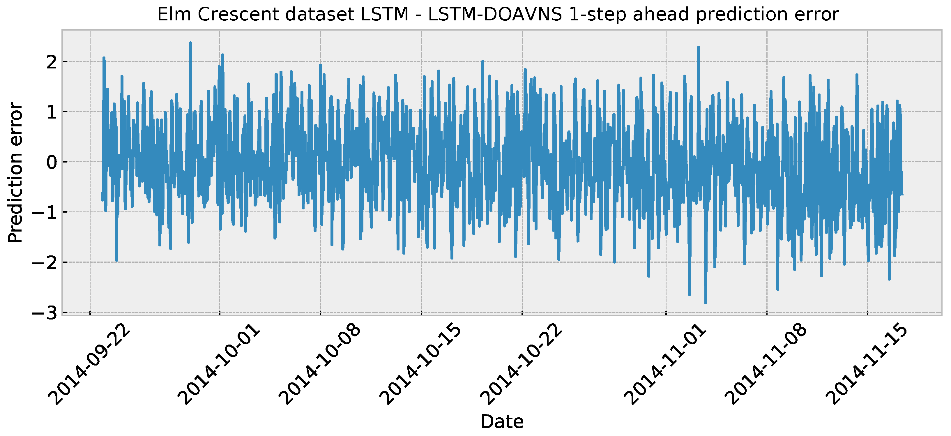
Figure 22. Elm Crescent LSTM simulations’ error over time.

5.2.2. LSTM Forest Road Simulations

Comparisons in terms of the objective function for Forest Road LSTM simulation scores are presented in Table 11. The introduced optimizer attained the best-performing model, scoring an objective function result of 0.007066 . The optimizer also scores highly in terms of the mean and median. However, the RSA attains the best outcome in the worst-case simulation. The GA showcases the highest stability rating. Further stability comparisons are provided in terms of objective and indicator score distribution diagrams for the objective function in Figure 23 and indicator function in Figure 24. A slight drop in stability can be observed for the introduced optimizer. This is to be somewhat expected with increasing diversification. Nevertheless, these modifications also allow the optimizer to avoid local optima, attaining overall better results in comparison to other tested algorithms.
Table 11. Forest Road LSTM simulations’ objective function outcomes.
Figure 23. Forest Road LSTM simulations’ objective function distribution diagrams.
Figure 24. Forest Road LSTM simulations’ indicator function distribution diagrams.
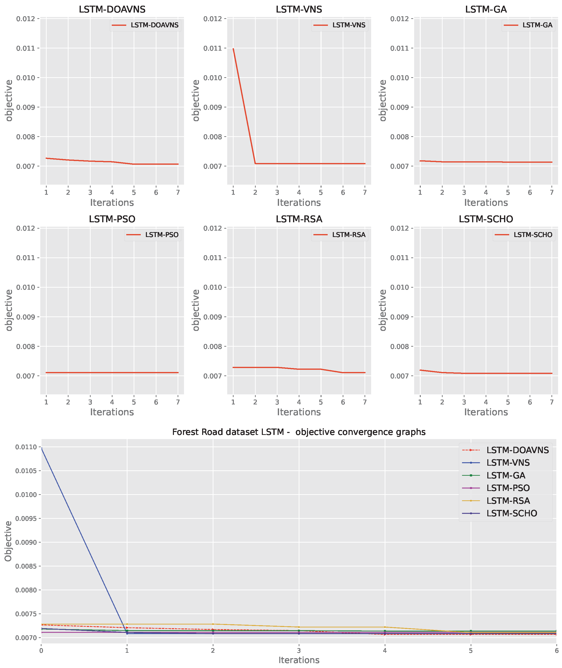
Further comparisons in terms of detailed metrics are provided in Table 12. The model optimized by the introduced DOAVNS optimizer showcases the best scores in terms of all metrics in the conducted tests.
Table 12. Forest Road LSTM simulations’ detailed metrics for the best-performing optimized models.
Convergence diagrams for each optimizer are provided in Figure 25 and Figure 26 for objective and indicator scores. The introduced optimizer overcomes a local optimum and converges toward a better solution, outperforming competing optimizers.
Figure 25. Forest Road LSTM simulations’ objective function convergence diagrams.
Figure 26. Forest Road LSTM simulations’ indicator function convergence diagrams.
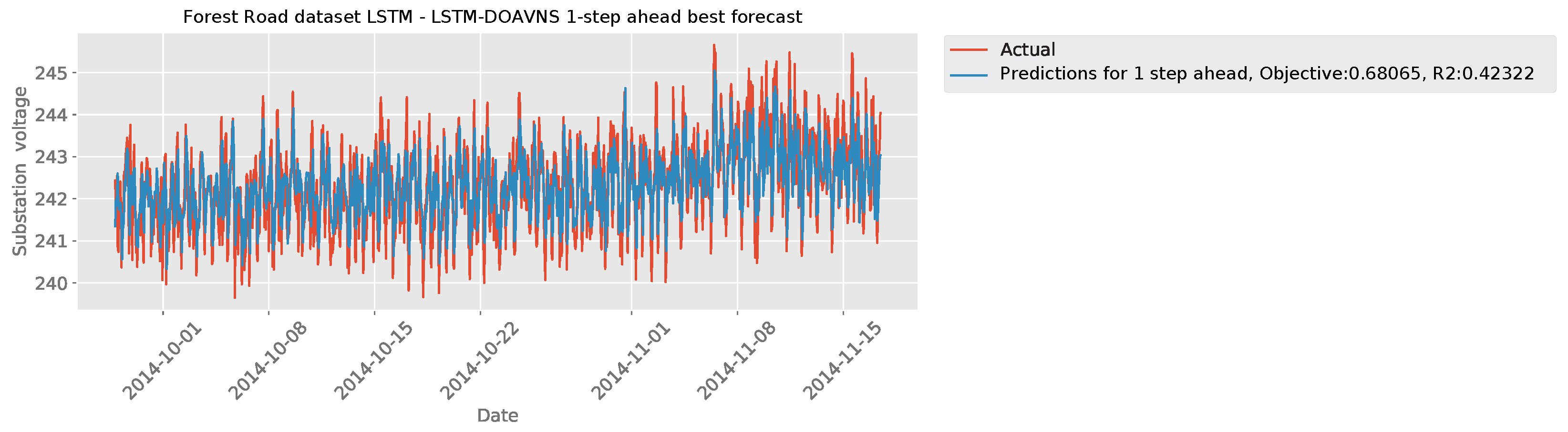
The parameter selections made by each algorithm for the respective best-performing model are provided in Table 13 to facilitate simulation repeatability. The predictions made by the best-performing model are provided in Figure 27, while Figure 28 provides insight into the error over time.
Table 13. Best-performing LSTM model parameter selections for Forest Road simulations.
Figure 27. Forecasts of best DOAVNS model from Forest Road LSTM simulations.
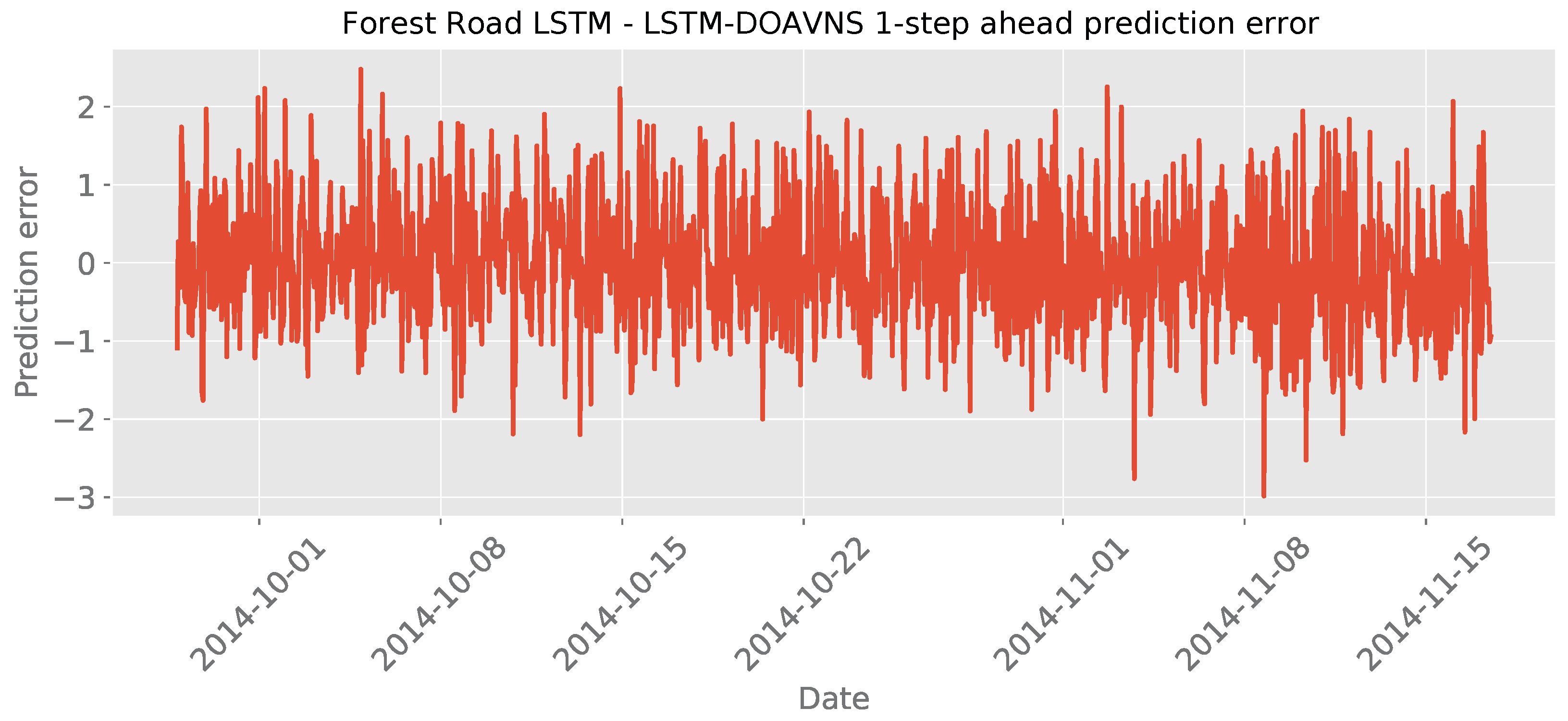
Figure 28. Forest Road LSTM simulations’ error over time.
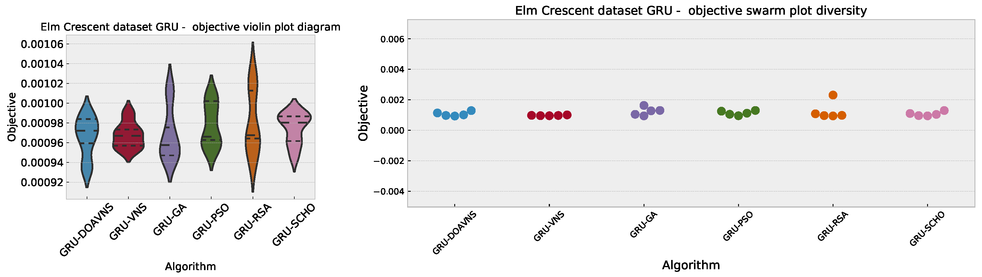
5.3. GRU Simulations

5.3.1. GRU Elm Crescent Simulations

Comparisons in terms of the objective function for Elm Crescent GRU simulation scores are presented in Table 14. The introduced optimizer attained the best-performing model, scoring an objective function result of 0.000935 , as well as the best worst-case and mean scores. However, the best median performance goes to the GA. Stability rates are best maintained by the VNA algorithm, despite the models not attaining high scores in other metrics. Further stability comparisons are provided in terms of objective and indicator score distribution diagrams for the objective function in Figure 29 and indicator function in Figure 30. A notable drop in stability can be observed for the introduced optimizer. However, as previously stated, this drop can be attributed to the boost in diversification.
Table 14. Elm Crescent GRU simulations’ objective function outcomes.
Figure 29. Elm Crescent GRU simulations’ objective function distribution diagrams.
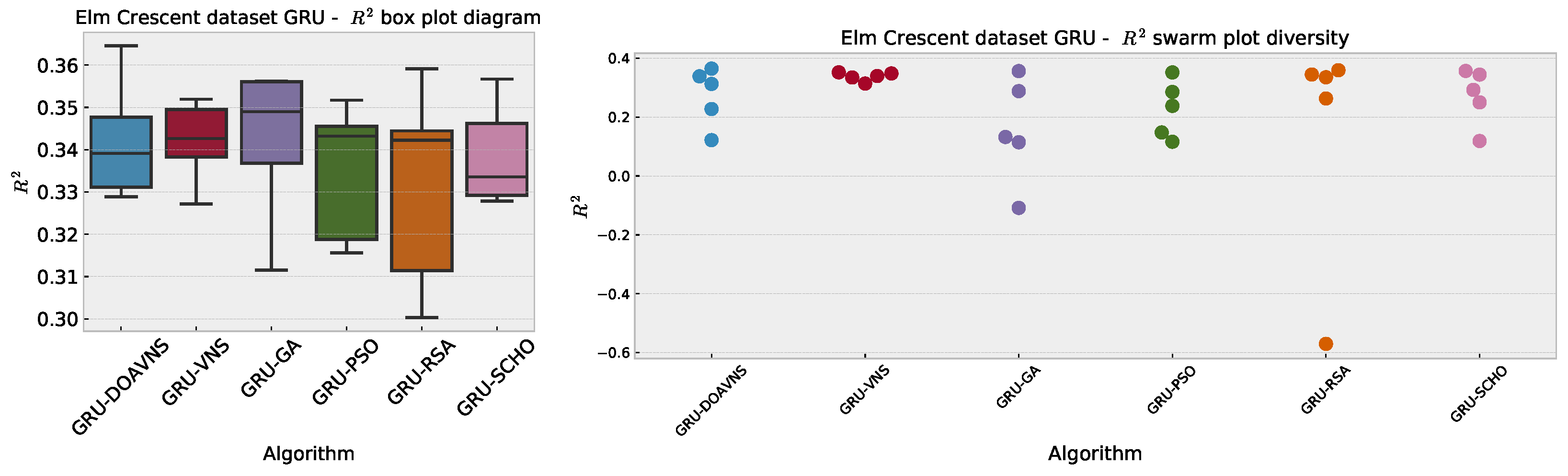
Figure 30. Elm Crescent GRU simulations’ indicator function distribution diagrams.
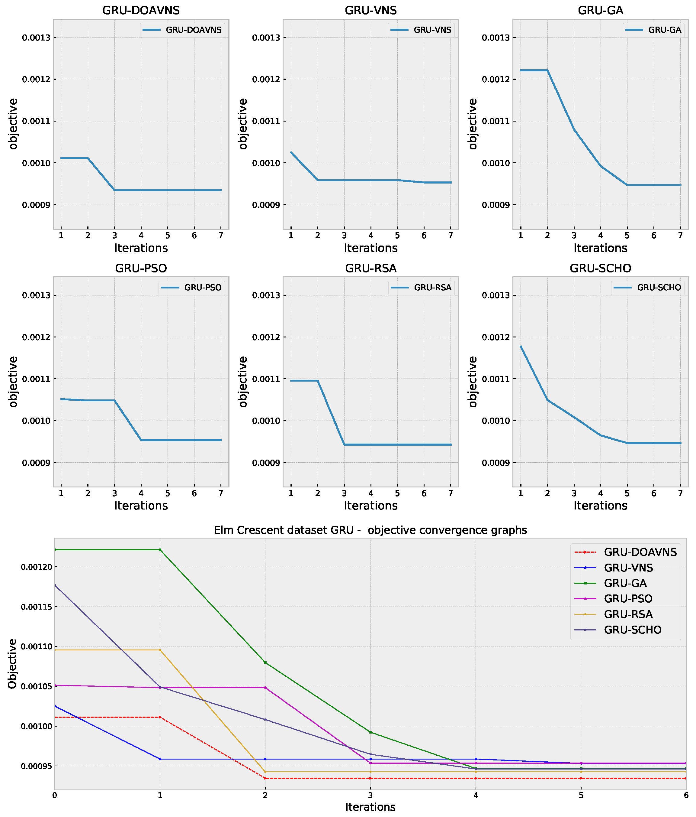
Further comparisons in terms of detailed metrics are provided in Table 15. The model optimized by the introduced DOAVNS optimizer showcases the best scores in terms of all metrics in the conducted tests.
Table 15. Elm Crescent GRU simulations’ detailed metrics for the best-performing optimized models.
Convergence diagrams for each optimizer are provided in Figure 31 and Figure 32 for objective and indicator scores. The introduced optimizer overcomes a local optimum and converges toward a better solution, outperforming competing optimizers.
Figure 31. Elm Crescent GRU simulations’ objective function convergence diagrams.
Figure 32. Elm Crescent GRU simulations’ indicator function convergence diagrams.
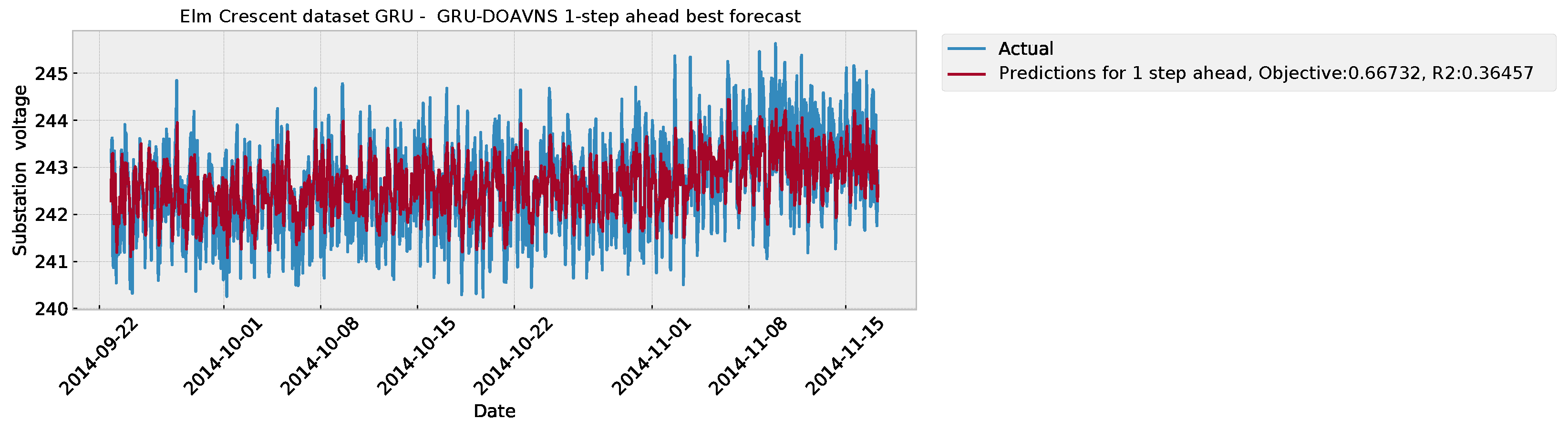
The parameter selections made by each algorithm for the respective best-performing model are provided in Table 16 to facilitate simulation repeatability. The predictions made by the best-performing model are provided in Figure 33. The plot of the error over time is given in Figure 34.
Table 16. Best-performing GRU model parameter selections for Elm Crescent simulations.
Figure 33. Forecasts of best DOAVNS model from Elm Crescent GRU simulations.
Figure 34. Elm Crescent GRU simulations’ error over time.
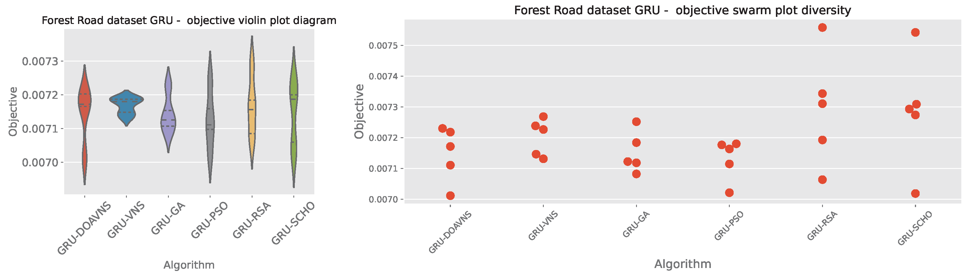
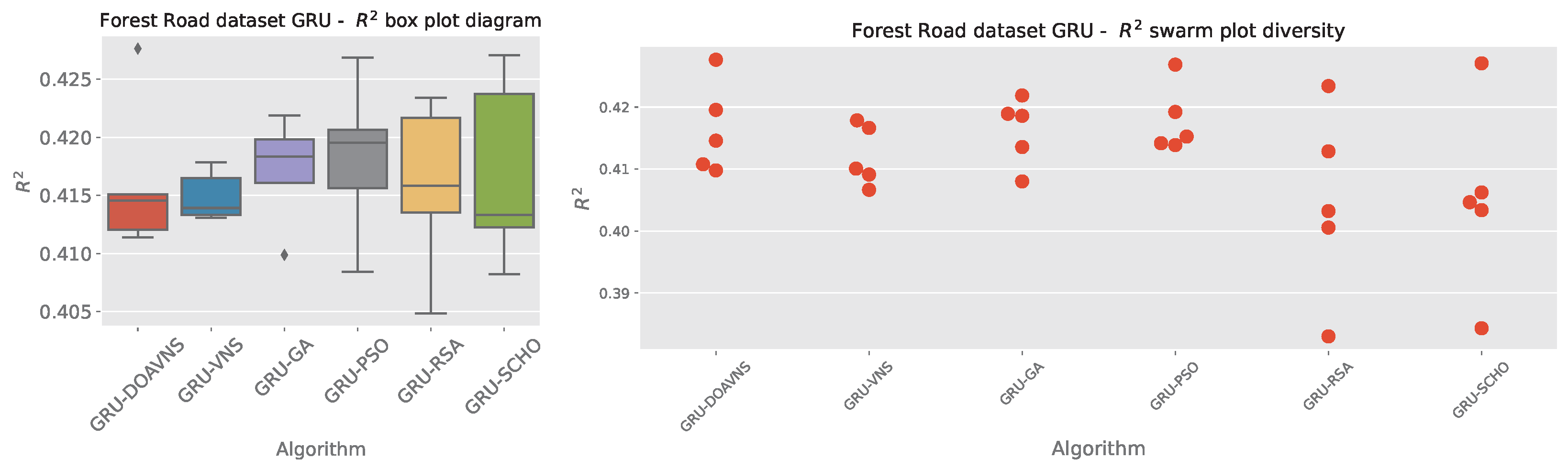
5.3.2. GRU Forest Road Simulations

Comparisons in terms of the objective function for Forest Road GRU simulation scores are presented in Table 17. While the introduced optimizer showcases the best outcome in terms of best-case executions with a score of 0.007011 , the other optimizers showcase good performance as well, with the VNS scoring highest in terms of worst-case outcomes, while the PSO has high scores in terms of the median and mean, and the VNS optimizer has the highest rate of stability. Further stability comparisons are provided in terms of objective and indicator score distribution diagrams for the objective function in Figure 35 and indicator function in Figure 36. A notable drop in stability can be observed for the introduced optimizer. However, as previously stated, this drop can be attributed to the boost in diversification.
Table 17. Forest Road GRU simulations’ objective function outcomes.
Figure 35. Forest Road GRU simulations’ objective function distribution diagrams.
Figure 36. Forest Road GRU simulations’ indicator function distribution diagrams.
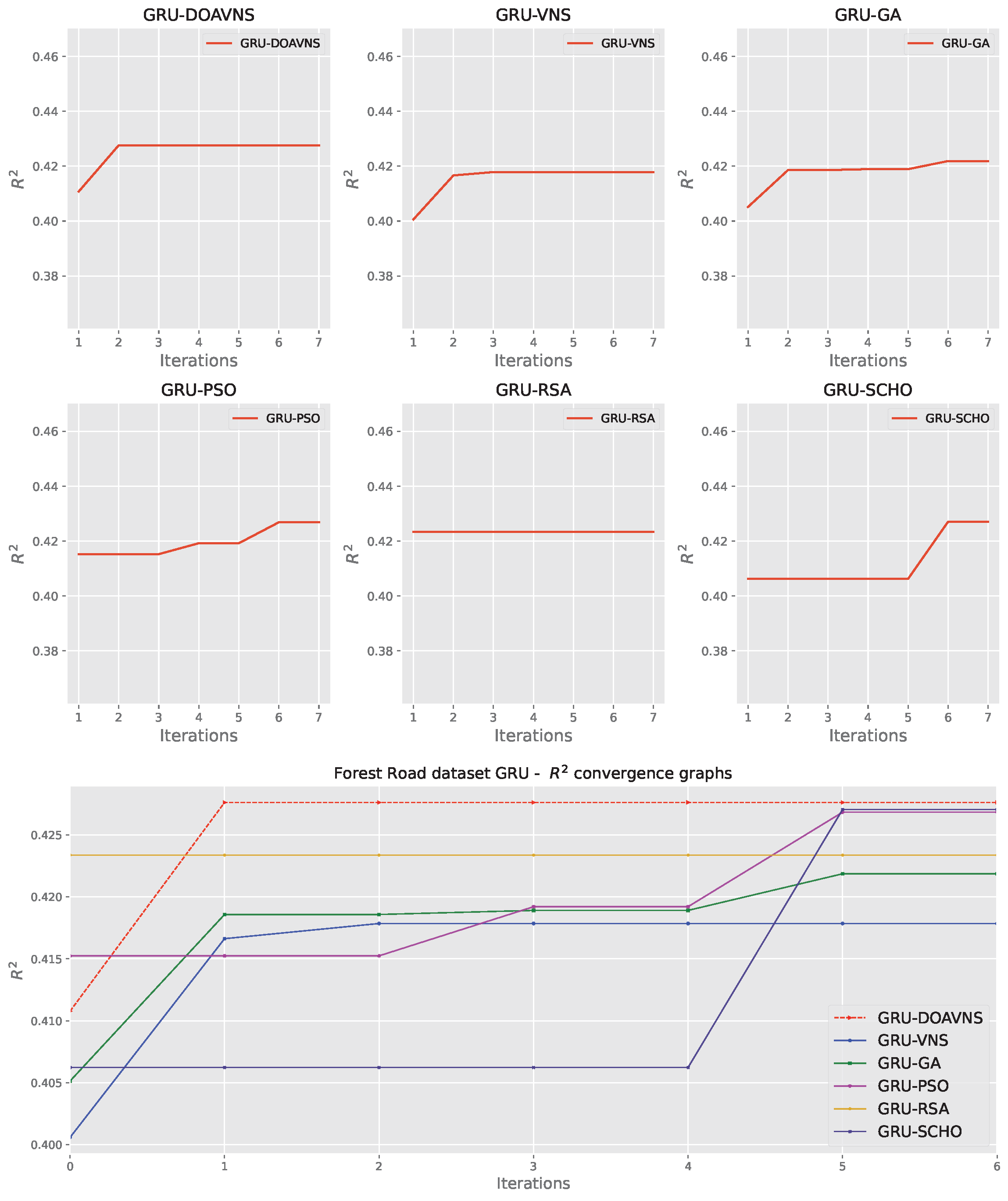
Further comparisons in terms of detailed metrics are provided in Table 18. The model optimized by the introduced DOAVNS optimizer showcases the best scores in terms of all metrics in the conducted tests. The introduced optimizer scores the highest in terms of R2, MSE, and RMSE. However, the RSA shows admirable performance in terms of MAE as well as the IoA.
Table 18. Forest Road GRU simulations’ detailed metrics for the best-performing optimized models.
Convergence diagrams for each optimizer are provided in Figure 37 and Figure 38 for objective and indicator scores. The introduced optimizer overcomes a local optimum and converges toward a better solution, outperforming competing optimizers.
Figure 37. Forest Road GRU simulations’ objective function convergence diagrams.
Figure 38. Forest Road GRU simulations’ indicator function convergence diagrams.
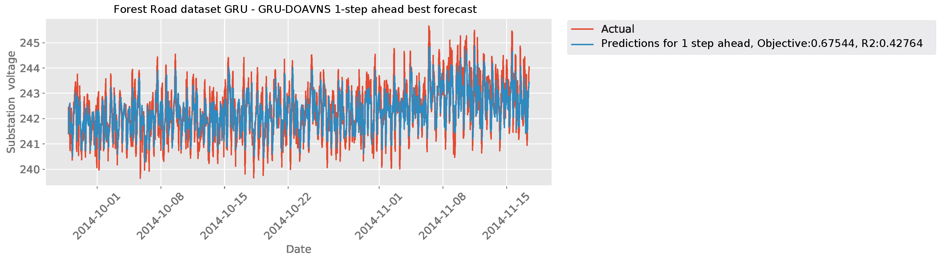
The parameter selections made by each algorithm for the respective best-performing model are provided in Table 19 to facilitate simulation repeatability. The predictions made by the best-performing model are provided in Figure 39. Lastly, Figure 40 plots the error over time.
Table 19. Best-performing GRU model parameter selections for Forest Road simulations.
Figure 39. Forecasts of best DOAVNS model from Forest Road GRU simulations.
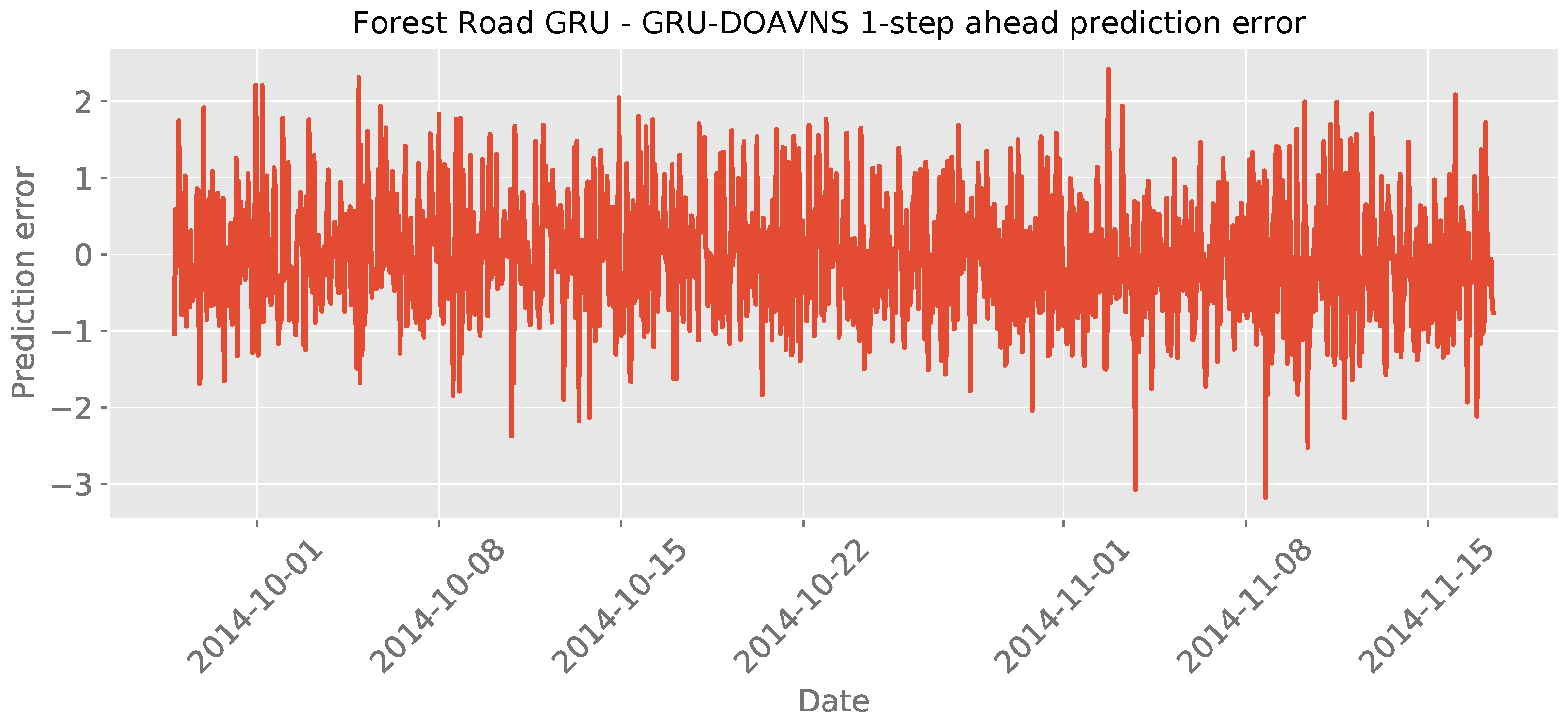
Figure 40. Forest Road GRU simulations’ error over time.
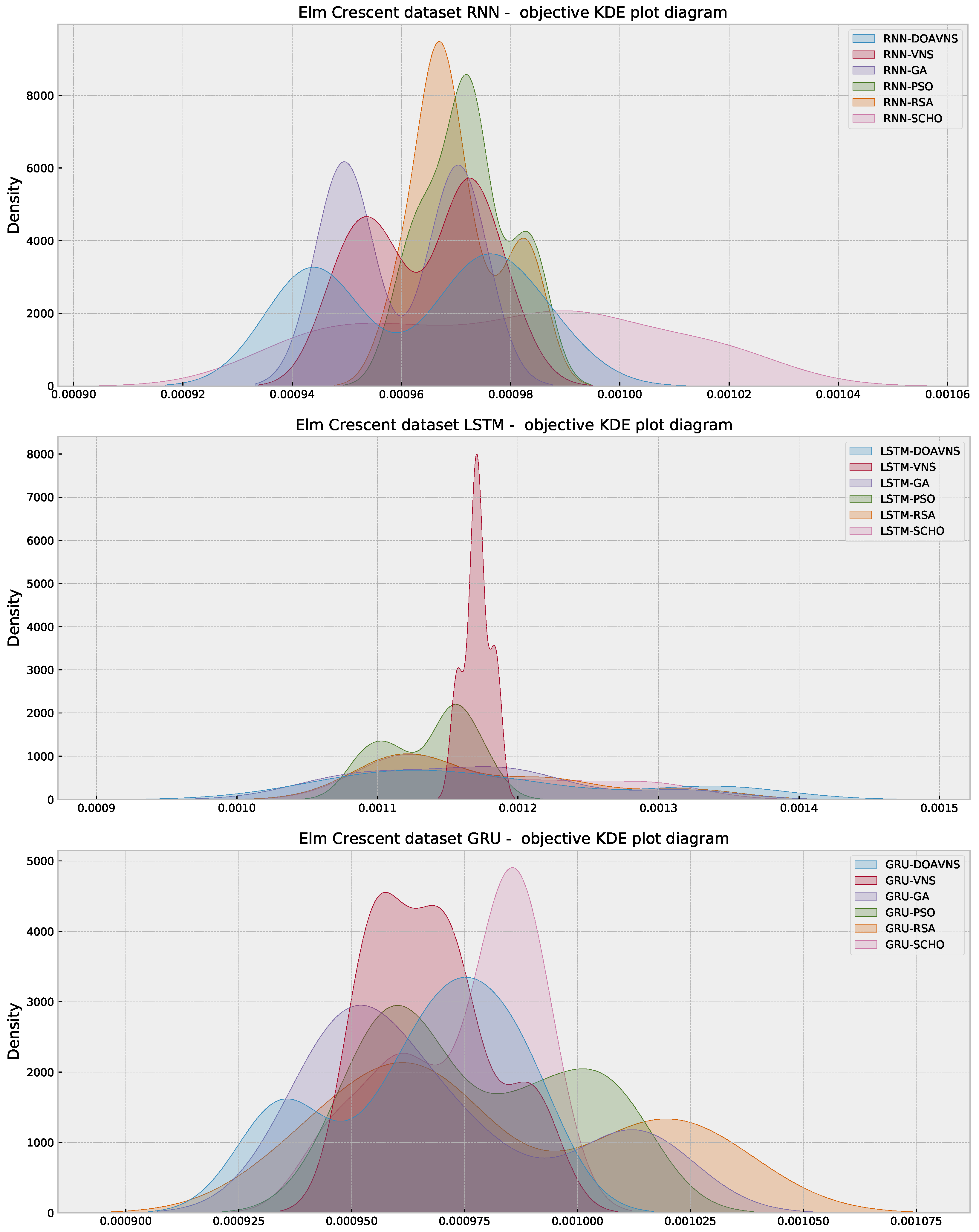
5.4. Comparison Between Best-Performing Models

A comparison between the best-performing optimized models in each simulation is presented in Table 20. The attained outcomes suggest that for the Elm Crescent dataset simulation, the GRU model showcases the best performance, with an R2 score of 0.364567 and an MSE of 0.000935 . In the case of Forest Road simulations, the GRU model also showcases the best scores, with an R2 of 0.427637 and an MSE of 0.007011 . Nevertheless, it is important to consider several factors when deciding on the most suitable model for use. The favorable performance of GRU makes these networks ideal for use in TinyML applications due to their relatively low computational demands in comparison to LSTM modes while still showing higher robustness and resistance to common issues in simple RNNs. For this reason, the GRU models are chosen for simulations with ESP32 devices, developed by Espressif Systems, a Chinese company based in Shanghai, China, and manufactured by TSMC using their 40 nm process.
Table 20. A comparison between the best-performing models in each simulation.

5.5. Optimization Statistical Validation

To establish a comparison between the evaluated algorithms, statistical validation is necessary, as relying on simple one-time executions can provide misleading conclusions. The conducted simulations need to meet an established set of criteria in order to be eligible for evaluation using parametric testing. Otherwise, non-parametric tests need to be utilized [58]. A sufficient number of simulations is needed to conduct testing; therefore, 30 turns were conducted for each of the conducted experiments, with independent random seeds satisfying the independence criteria. Homoscedasticity was established via Levene’s test [59], where the resulting p values are 0.62 for each of the simulations, suggesting this criterion is also met. Finally, the normality criterion was tested with the Shapiro–Wilk [60] test. The attained outcomes are presented in Table 21. With the attained values falling below 0.05 , the null hypothesis is rejected, suggesting that the normality assumption is not satisfied, and parametric test usage cannot be justified. Normality observations are further confirmed by the objective function KDE diagrams presented in Figure 41 and Figure 42 for Elm Crescent and Forest Road simulations.
Table 21. Shapiro–Wilk scores for forecasting experiments for normality condition evaluation.
Figure 41. Elm Crescent simulation KDE diagrams.
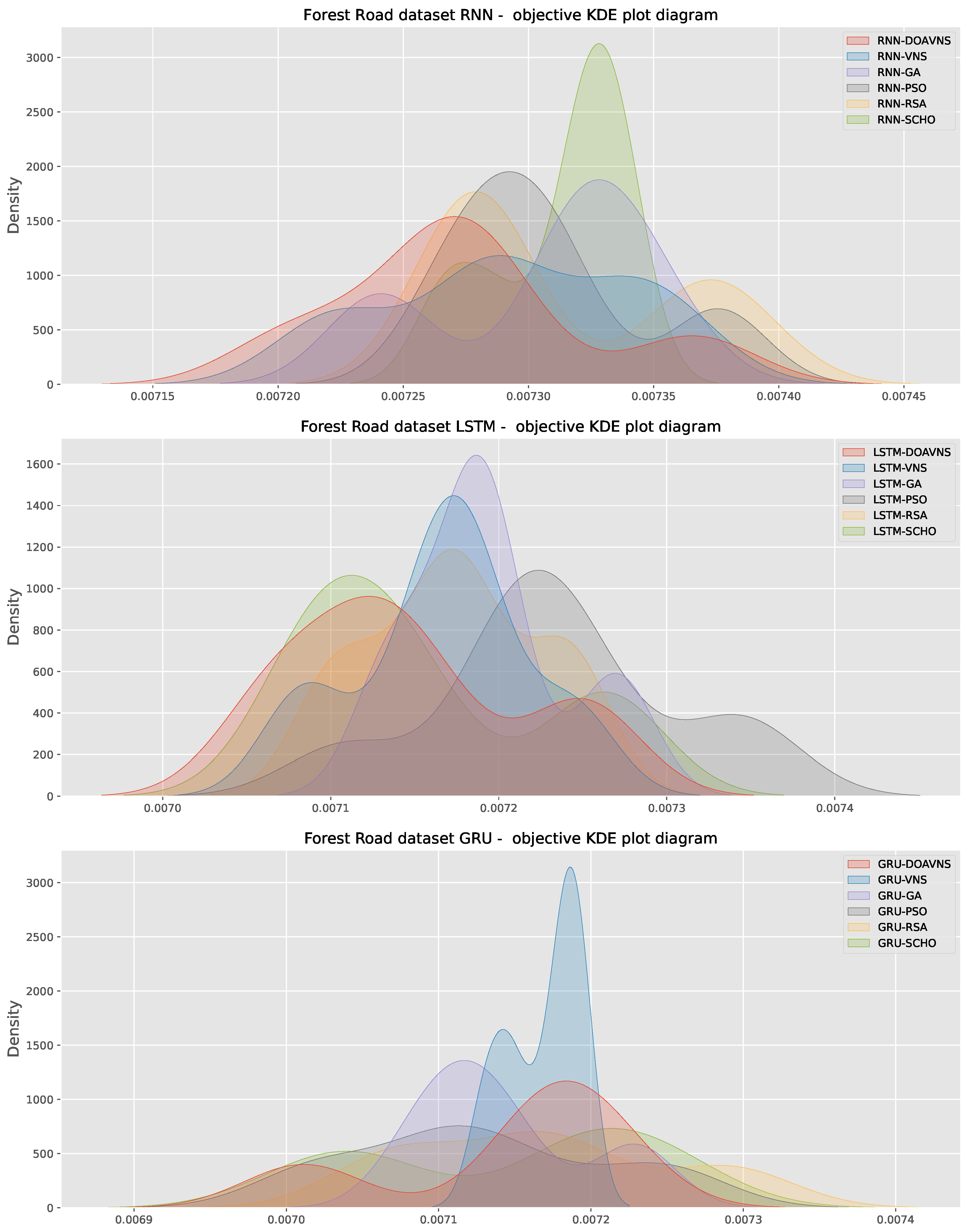
Figure 42. Forest road simulation KDE diagrams.
As the conditions needed for parametric test application were not met, this work resorted to the utilization of the Wilcoxon signed-rank test [61] to establish a comparison between the proposed DOAVNS and other optimizers. The outcomes of this test are outlined in Table 22. As all criteria fall below the threshold limit α = 0.05 , the attained outcomes suggest the statistical significance of the attained comparative analysis scores.
Table 22. Wilcoxon signed-rank test scores in forecasting experiments.

5.6. Deployment Simulations

Based on simulation outcomes, GRU models showcase optimal performance once optimized and trained for prediction in both simulation cases. This is favorable, as the lower computational demands of GRUs make them ideal for deployment on MCUs that face challenges with limited computational resources. In this study, the models were re-implemented using TensorFlow Lite, compiled, converted to C, and uploaded to an ESP32 development board using the Arduino IDE. The device is configured to monitor a serial port input and, based on a series of inputs, generates responses accordingly. Simulations using the test portion of the datasets yield results consistent with the scores reported in prior tables, suggesting viability for real-world use.
It is important to note that the ESP32 supports additional configurations, such as a web server and the direct monitoring of voltages using a step-down transformer or external ADC, which could also be integrated with the platform. The proof-of-concept study conducted in this work suggests that an expanded version of this system could significantly aid in the distribution and democratization of IoT devices for energy forecasting, thereby improving renewable energy integration into existing power distribution networks and reducing losses from power overproduction and distribution.

6. Conclusions

With limited fossil resources and their unsustainable impacts, there is an increasing shift toward renewable energy. However, successfully incorporating these new sources into current power grids remains challenging, with both technical and regulatory obstacles to address. Although enhancing reliability could greatly improve energy sustainability, solar energy’s reliance on weather introduces variability that often requires costly storage to ensure stable output.
This study focuses on leveraging metaheuristic optimization to fine-tune recurrent forecasting models aimed at predicting solar power production, designed for TinyML deployment on MCUs in in situ applications. Various recurrent models—RNN, LSTM, and GRU—were tested to identify the most effective model. Additionally, a comparative evaluation on two real-world datasets for separate locations was conducted, encompassing multiple optimizers to validate the approach; a custom optimizer showed promising results, achieving an MSE as low as 0.000935v and 0.007011v in the best-case scenarios on the two evaluated datasets, signaling its potential for real-world implementation. The best models were further assessed on an ESP32 chip, utilizing a UART terminal to simulate execution. Model performance was consistent, with minimal latency for the application’s needs. By deploying models directly on-site, network infrastructure costs are reduced, and local functionalities can be added to help manage demand and supply more effectively, including alerting in critical situations.
One drawback is that, in this setup, models deployed on MCUs cannot be updated in real time; instead, they require retraining on separate hardware and reprogramming MCU firmware for updates. Other limitations include restricted population sizes and optimization times, given the high computational load. Future research aims to extend this methodology, exploring broader applications for the optimized model and developing the experimental framework within the TinyML environment. Specific directions will include the implementation of real-time model updates, the integration of wireless sensor networks, and the development of distributed forecasting systems over different renewable energy sources like wind, hydroelectric, and solar power. The research will also examine a solar power dataset from the Balkans, which is currently being collected; however, it is currently neither openly available nor complete for experiments of this scale. Ultimately, the application of TinyML models will be extended to other application domains, including healthcare, agriculture, IoT security, and industry, where these models may help in image classification, wireless sensor network routing, fault detection, fall prediction for children and elderly persons, etc.

Policy Implications

Precise TinyML-based solar energy forecasting systems can significantly impact legal policies related to grid reliability and renewable energy integration in the Western Balkans. By providing accurate, localized forecasts, these systems enhance compliance with EU regulations, like RED II, which promotes greater renewable energy use and efficient grid integration. Such models support policies aimed at improving grid stability by balancing renewable energy supply and demand, aligning with national energy security and greenhouse gas reduction goals set forth in NECPs. Furthermore, precise in situ forecasts can help reduce reliance on fossil fuel backups during periods of fluctuating solar output, advancing both regional and EU emission reduction targets.
TinyML’s cost-effective, localized deployment enables decentralized monitoring, reducing the need for extensive networking infrastructure and making renewable integration more accessible, particularly for smaller towns and remote areas. Building on incentives like feed-in tariffs, this capability could prompt policymakers to offer financial support for TinyML within larger renewable energy subsidies. Moreover, TinyML supports continuous monitoring and analysis of real-time data coming from sensors, which can aid in the identification of patterns indicating anomalies, like equipment malfunctioning or deviations in electricity output, ensuring fast interventions and reducing system downtime. Continuous monitoring can help in the integration of renewable systems with smart grids, ensuring that energy production matches demand and stabilizing the grid through predictions of energy fluctuations. Improved monitoring and storage capabilities enabled by TinyML could also support cross-border energy exchange regulations. With more accurate forecasting of production surpluses, energy can be stored or traded internationally, aiding regional energy independence, lowering reliance on imports, and achieving the Energy Community’s goal of harmonized market integration across the Western Balkans.
Finally, TinyML’s predictive accuracy aligns with environmental protection regulations by enabling solar projects to anticipate and mitigate environmental impacts more effectively. Accurate production models ensure compliance with air quality and resource conservation standards, expediting environmental impact assessments under regulations like the Environmental Protection Law. By integrating TinyML, regulatory oversight could become more efficient through real-time data that identify inefficiencies or excessive emissions. TinyML thus has the potential to drive policies supporting a resilient and sustainable energy grid across the Western Balkans, equipping decision-makers with improved monitoring and forecasting tools.

Author Contributions

Conceptualization, G.P., L.S. and L.J.; methodology, N.B.; software, N.B.; validation, N.B., M.Z. and Z.S.; formal analysis, M.Z.; investigation, M.Z.; resources, L.J.; data curation, L.J.; writing—original draft preparation, Z.S.; writing—review and editing, G.P.; visualization, M.Z.; supervision, Z.S.; project administration, N.B.; funding acquisition, L.S. All authors have read and agreed to the published version of the manuscript.

Funding

This research received no external funding.

Data Availability Statement

The data utilized in this work are publicly available at https://www.kaggle.com/datasets/pythonafroz/solar-panel-energy-generation-data (accessed on 25 October 2024); Code snippets from the framework and datasets that were used for testing are available on the following github URL: https://github.com/nbacanin/solarforecastingtinyml (accessed on 25 October 2024).

Conflicts of Interest

The authors declare no conflicts of interest.

References

  1. Höök, M.; Tang, X. Depletion of fossil fuels and anthropogenic climate change—A review. Energy Policy 2013, 52, 797–809. [Google Scholar] [CrossRef]
  2. Hayat, M.B.; Ali, D.; Monyake, K.C.; Alagha, L.; Ahmed, N. Solar energy—A look into power generation, challenges, and a solar-powered future. Int. J. Energy Res. 2019, 43, 1049–1067. [Google Scholar] [CrossRef]
  3. Hassan, Q.; Algburi, S.; Sameen, A.Z.; Salman, H.M.; Jaszczur, M. A review of hybrid renewable energy systems: Solar and wind-powered solutions: Challenges, opportunities, and policy implications. Results Eng. 2023, 20, 101621. [Google Scholar] [CrossRef]
  4. Simankov, V.; Buchatskiy, P.; Kazak, A.; Teploukhov, S.; Onishchenko, S.; Kuzmin, K.; Chetyrbok, P. A Solar and Wind Energy Evaluation Methodology Using Artificial Intelligence Technologies. Energies 2024, 17, 416. [Google Scholar] [CrossRef]
  5. European Parliament and Council of the European Union. Directive (EU) 2018/2001 of the European Parliament and of the Council on the Promotion of the Use of Energy from Renewable Sources (Recast); Text with EEA relevance; European Parliament and Council of the European Union: Brussels, Belgium, 2018. [Google Scholar]
  6. European Commission. EU’s Revised Renewable Energy Directive. 2018. Available online: https://eur-lex.europa.eu/eli/dir/2018/2001/oj (accessed on 31 October 2024).
  7. Lim, B.; Zohren, S. Time-series forecasting with deep learning: A survey. Philos. Trans. R. Soc. A 2021, 379, 20200209. [Google Scholar] [CrossRef]
  8. Kataray, T.; Nitesh, B.; Yarram, B.; Sinha, S.; Cuce, E.; Shaik, S.; Vigneshwaran, P.; Roy, A. Integration of smart grid with renewable energy sources: Opportunities and challenges—A comprehensive review. Sustain. Energy Technol. Assess. 2023, 58, 103363. [Google Scholar] [CrossRef]
  9. Khalid, M. Smart grids and renewable energy systems: Perspectives and grid integration challenges. Energy Strategy Rev. 2024, 51, 101299. [Google Scholar] [CrossRef]
  10. Berta, R.; Dabbous, A.; Lazzaroni, L.; Pau, D.; Bellotti, F. Developing a TinyML Image Classifier in a Hour. IEEE Open J. Ind. Electron. Soc. 2024, 5, 946–960. [Google Scholar] [CrossRef]
  11. Ficco, M.; Guerriero, A.; Milite, E.; Palmieri, F.; Pietrantuono, R.; Russo, S. Federated learning for IoT devices: Enhancing TinyML with on-board training. Inf. Fusion 2024, 104, 102189. [Google Scholar] [CrossRef]
  12. Elhanashi, A.; Dini, P.; Saponara, S.; Zheng, Q. Advancements in TinyML: Applications, Limitations, and Impact on IoT Devices. Electronics 2024, 13, 3562. [Google Scholar] [CrossRef]
  13. Medsker, L.; Jain, L.C. Recurrent Neural Networks: Design and Applications; CRC Press: Boca Raton, FL, USA, 1999. [Google Scholar]
  14. Bischl, B.; Binder, M.; Lang, M.; Pielok, T.; Richter, J.; Coors, S.; Thomas, J.; Ullmann, T.; Becker, M.; Boulesteix, A.L.; et al. Hyperparameter optimization: Foundations, algorithms, best practices, and open challenges. Wiley Interdiscip. Rev. Data Min. Knowl. Discov. 2023, 13, e1484. [Google Scholar] [CrossRef]
  15. Alazemi, T.; Darwish, M.; Radi, M. Renewable energy sources integration via machine learning modelling: A systematic literature review. Heliyon 2024, 10, e26088. [Google Scholar] [CrossRef] [PubMed]
  16. Khurshid, H.; Mohammed, B.S.; Al-Yacoubya, A.M.; Liew, M.; Zawawi, N.A.W.A. Analysis of hybrid offshore renewable energy sources for power generation: A literature review of hybrid solar, wind, and waves energy systems. Dev. Built Environ. 2024, 19, 100497. [Google Scholar] [CrossRef]
  17. Bacanin, N.; Jovanovic, L.; Zivkovic, M.; Kandasamy, V.; Antonijevic, M.; Deveci, M.; Strumberger, I. Multivariate energy forecasting via metaheuristic tuned long-short term memory and gated recurrent unit neural networks. Inf. Sci. 2023, 642, 119122. [Google Scholar] [CrossRef]
  18. Park, K.; Yim, J.; Lee, H.; Park, M.; Kim, H. Real-time solar power estimation through rnn-based attention models. IEEE Access 2023, 12, 62502–62510. [Google Scholar] [CrossRef]
  19. Zameer, A.; Jaffar, F.; Shahid, F.; Muneeb, M.; Khan, R.; Nasir, R. Short-term solar energy forecasting: Integrated computational intelligence of LSTMs and GRU. PLoS ONE 2023, 18, e0285410. [Google Scholar] [CrossRef]
  20. Moradzadeh, A.; Moayyed, H.; Mohammadi-Ivatloo, B.; Vale, Z.; Ramos, C.; Ghorbani, R. A novel cyber-Resilient solar power forecasting model based on secure federated deep learning and data visualization. Renew. Energy 2023, 211, 697–705. [Google Scholar] [CrossRef]
  21. Salman, D.; Direkoglu, C.; Kusaf, M.; Fahrioglu, M. Hybrid deep learning models for time series forecasting of solar power. Neural Comput. Appl. 2024, 36, 9095–9112. [Google Scholar] [CrossRef]
  22. Olcay, K.; Tunca, S.G.; Özgür, M.A. Forecasting and performance analysis of energy production in solar power plants using long short-term memory (LSTM) and random forest models. IEEE Access 2024, 12, 103299–103312. [Google Scholar] [CrossRef]
  23. Jailani, N.L.M.; Dhanasegaran, J.K.; Alkawsi, G.; Alkahtani, A.A.; Phing, C.C.; Baashar, Y.; Capretz, L.F.; Al-Shetwi, A.Q.; Tiong, S.K. Investigating the power of LSTM-based models in solar energy forecasting. Processes 2023, 11, 1382. [Google Scholar] [CrossRef]
  24. Guo, X.; Zhan, Y.; Zheng, D.; Li, L.; Qi, Q. Research on short-term forecasting method of photovoltaic power generation based on clustering SO-GRU method. Energy Rep. 2023, 9, 786–793. [Google Scholar] [CrossRef]
  25. Xu, Y.; Zheng, S.; Zhu, Q.; Wong, K.c.; Wang, X.; Lin, Q. A complementary fused method using GRU and XGBoost models for long-term solar energy hourly forecasting. Expert Syst. Appl. 2024, 254, 124286. [Google Scholar] [CrossRef]
  26. Hayajneh, A.M.; Alasali, F.; Salama, A.; Holderbaum, W. Intelligent Solar Forecasts: Modern Machine Learning Models & TinyML Role for Improved Solar Energy Yield Predictions. IEEE Access 2024, 12, 10846–10864. [Google Scholar]
  27. Yang, L.; Shami, A. On hyperparameter optimization of machine learning algorithms: Theory and practice. Neurocomputing 2020, 415, 295–316. [Google Scholar] [CrossRef]
  28. Bassey, K.E. Hybrid renewable energy systems modeling. Eng. Sci. Technol. J. 2023, 4, 571–588. [Google Scholar] [CrossRef]
  29. Öcal, A.; Koyuncu, H. An in-depth study to fine-tune the hyperparameters of pre-trained transfer learning models with state-of-the-art optimization methods: Osteoarthritis severity classification with optimized architectures. Swarm Evol. Comput. 2024, 89, 101640. [Google Scholar] [CrossRef]
  30. Kennedy, J.; Eberhart, R. Particle swarm optimization. In Proceedings of the Proceedings of ICNN’95—International Conference on Neural Networks, Perth, WA, Australia, 27 November–1 December 1995; Volume 4, pp. 1942–1948. [Google Scholar] [CrossRef]
  31. Mirjalili, S. Genetic Algorithm. In Evolutionary Algorithms and Neural Networks: Theory and Applications; Springer International Publishing: Cham, Switzerland, 2019; pp. 43–55. [Google Scholar] [CrossRef]
  32. Abualigah, L.; Elaziz, M.A.; Sumari, P.; Geem, Z.W.; Gandomi, A.H. Reptile Search Algorithm (RSA): A nature-inspired meta-heuristic optimizer. Expert Syst. Appl. 2022, 191, 116158. [Google Scholar] [CrossRef]
  33. Bai, J.; Li, Y.; Zheng, M.; Khatir, S.; Benaissa, B.; Abualigah, L.; Abdel Wahab, M. A Sinh Cosh optimizer. Knowl.-Based Syst. 2023, 282, 111081. [Google Scholar] [CrossRef]
  34. Minic, A.; Jovanovic, L.; Bacanin, N.; Stoean, C.; Zivkovic, M.; Spalevic, P.; Petrovic, A.; Dobrojevic, M.; Stoean, R. Applying recurrent neural networks for anomaly detection in electrocardiogram sensor data. Sensors 2023, 23, 9878. [Google Scholar] [CrossRef]
  35. Jovanovic, L.; Djuric, M.; Zivkovic, M.; Jovanovic, D.; Strumberger, I.; Antonijevic, M.; Budimirovic, N.; Bacanin, N. Tuning xgboost by planet optimization algorithm: An application for diabetes classification. In Proceedings of the Fourth International Conference on Communication, Computing and Electronics Systems: ICCCES 2022, Coimbatore, India, 15–16 September 2022; Springer: Berlin/Heidelberg, Germany, 2023; pp. 787–803. [Google Scholar]
  36. Jovanovic, L.; Bacanin, N.; Zivkovic, M.; Antonijevic, M.; Petrovic, A.; Zivkovic, T. Anomaly detection in ECG using recurrent networks optimized by modified metaheuristic algorithm. In Proceedings of the 2023 31st Telecommunications Forum (TELFOR), Belgrade, Serbia, 21–22 November 2023; pp. 1–4. [Google Scholar]
  37. Mladenovic, D.; Antonijevic, M.; Jovanovic, L.; Simic, V.; Zivkovic, M.; Bacanin, N.; Zivkovic, T.; Perisic, J. Sentiment classification for insider threat identification using metaheuristic optimized machine learning classifiers. Sci. Rep. 2024, 14, 25731. [Google Scholar] [CrossRef]
  38. Dobrojevic, M.; Jovanovic, L.; Babic, L.; Cajic, M.; Zivkovic, T.; Zivkovic, M.; Muthusamy, S.; Antonijevic, M.; Bacanin, N. Cyberbullying Sexism Harassment Identification by Metaheurustics-Tuned eXtreme Gradient Boosting. Comput. Mater. Contin. 2024, 80, 4997–5027. [Google Scholar] [CrossRef]
  39. Pavlov-Kagadejev, M.; Jovanovic, L.; Bacanin, N.; Deveci, M.; Zivkovic, M.; Tuba, M.; Strumberger, I.; Pedrycz, W. Optimizing long-short-term memory models via metaheuristics for decomposition aided wind energy generation forecasting. Artif. Intell. Rev. 2024, 57, 45. [Google Scholar] [CrossRef]
  40. Damaševičius, R.; Jovanovic, L.; Petrovic, A.; Zivkovic, M.; Bacanin, N.; Jovanovic, D.; Antonijevic, M. Decomposition aided attention-based recurrent neural networks for multistep ahead time-series forecasting of renewable power generation. PeerJ Comput. Sci. 2024, 10, e1795. [Google Scholar] [CrossRef] [PubMed]
  41. Bacanin, N.; Petrovic, A.; Jovanovic, L.; Zivkovic, M.; Zivkovic, T.; Sarac, M. Parkinson’s Disease Induced Gain Freezing Detection using Gated Recurrent Units Optimized by Modified Crayfish Optimization Algorithm. In Proceedings of the 2024 5th International Conference on Mobile Computing and Sustainable Informatics (ICMCSI), Lalitpur, Nepal, 18–19 January 2024; pp. 1–8. [Google Scholar]
  42. Bacanin, N.; Jovanovic, L.; Djordjevic, M.; Petrovic, A.; Zivkovic, T.; Zivkovic, M.; Antonijevic, M. Crop Yield Forecasting Based on Echo State Network Tuned by Crayfish Optimization Algorithm. In Proceedings of the 2024 IEEE International Conference on Contemporary Computing and Communications (InC4), Bengaluru, India, 15–16 March 2024; Volume 1, pp. 1–6. [Google Scholar]
  43. Government of Montenegro. Zakon o Energetici. Available online: https://www.gov.me/dokumenta/d17f9f62-ea19-4dd2-a73f-cbf6bfffab5c (accessed on 31 October 2024).
  44. European Union. Communication on REPowerEU Plan. 2022. Available online: https://eur-lex.europa.eu/legal-content/EN/TXT/HTML/?uri=CELEX:52022DC0230 (accessed on 31 October 2024).
  45. Ekološka Ekonomija. Što je feed-in tarifa za obnovljive izvore? [What Is a Feed-in Tariff for Renewable Energy?]. 2016. Available online: https://ekoloskaekonomija.wordpress.com/2016/09/30/sto-je-feed-in-tarifa-za-obnovljive-izvore/ (accessed on 31 October 2024).
  46. D’Aprile, P.; Engel, H.; van Gendt, G.; Helmcke, S.; Hieronimus, S.; Nauclér, T.; Pinner, D.; Walter, D.; Witteveen, M. Net-Zero Europe: Decarbonization Pathways and Socioeconomic Implications; McKinsey & Company: Stockholm, Sweden, 2020. [Google Scholar]
  47. Sherstinsky, A. Fundamentals of recurrent neural network (RNN) and long short-term memory (LSTM) network. Phys. D Nonlinear Phenom. 2020, 404, 132306. [Google Scholar] [CrossRef]
  48. Chung, J.; Gulcehre, C.; Cho, K.; Bengio, Y. Empirical evaluation of gated recurrent neural networks on sequence modeling. In Proceedings of the NIPS 2014 Workshop on Deep Learning, Montreal, QC, Canada, 13 December 2014. [Google Scholar]
  49. Mladenović, N.; Hansen, P. Variable neighborhood search. Comput. Oper. Res. 1997, 24, 1097–1100. [Google Scholar] [CrossRef]
  50. Luo, W.; Lin, X.; Li, C.; Yang, S.; Shi, Y. Benchmark Functions for CEC 2022 Competition on Seeking Multiple Optima in Dynamic Environments. arXiv 2022, arXiv:cs.NE/2201.00523. [Google Scholar]
  51. Cheng, S.; Shi, Y. Diversity control in particle swarm optimization. In Proceedings of the 2011 IEEE Symposium on Swarm Intelligence, Paris, France, 11–15 April 2011; pp. 1–9. [Google Scholar] [CrossRef]
  52. Yang, X.S.; He, X. Firefly algorithm: Recent advances and applications. Int. J. Swarm Intell. 2013, 1, 36–50. [Google Scholar] [CrossRef]
  53. Espressif Systems. ESP32 Series Datasheet. 2024. Available online: https://www.espressif.com/en/products/socs/esp32 (accessed on 15 October 2024).
  54. Maier, A.; Sharp, A.; Vagapov, Y. Comparative analysis and practical implementation of the ESP32 microcontroller module for the internet of things. In Proceedings of the 2017 Internet Technologies and Applications (ITA), Wrexham, UK, 12–15 September 2017; pp. 143–148. [Google Scholar]
  55. Zim, M.Z.H. TinyML: Analysis of Xtensa LX6 microprocessor for neural network applications by ESP32 SoC. arXiv 2021, arXiv:2106.10652. [Google Scholar]
  56. Tatachar, A.V. Comparative assessment of regression models based on model evaluation metrics. Int. J. Innov. Technol. Explor. Eng. 2021, 8, 853–860. [Google Scholar]
  57. Willmott, C.J.; Robeson, S.M.; Matsuura, K. A refined index of model performance. Int. J. Climatol. 2012, 32, 2088–2094. [Google Scholar] [CrossRef]
  58. LaTorre, A.; Molina, D.; Osaba, E.; Poyatos, J.; Del Ser, J.; Herrera, F. A prescription of methodological guidelines for comparing bio-inspired optimization algorithms. Swarm Evol. Comput. 2021, 67, 100973. [Google Scholar] [CrossRef]
  59. Schultz, B.B. Levene’s Test for Relative Variation. Syst. Biol. 1985, 34, 449–456. [Google Scholar] [CrossRef]
  60. Shapiro, S.S.; Francia, R.S. An Approximate Analysis of Variance Test for Normality. J. Am. Stat. Assoc. 1972, 67, 215–216. [Google Scholar] [CrossRef]
  61. Woolson, R.F. Wilcoxon Signed-Rank Test. In Encyclopedia of Biostatistics; John Wiley & Sons, Ltd.: Hoboken, NJ, USA, 2005. [Google Scholar] [CrossRef]
Disclaimer/Publisher’s Note: The statements, opinions and data contained in all publications are solely those of the individual author(s) and contributor(s) and not of MDPI and/or the editor(s). MDPI and/or the editor(s) disclaim responsibility for any injury to people or property resulting from any ideas, methods, instructions or products referred to in the content.

Article Metrics

Citations

Article Access Statistics

Multiple requests from the same IP address are counted as one view.