Wind Turbine Wake Regulation Method Coupling Actuator Model and Engineering Wake Model

Abstract

The wake effect is one of the main factors affecting the power generation of wind farms. Wake regulation is often used to reduce the wake interference between wind turbines. Accurate assessment of the wake flow of wind turbine is essential to wake regulation. Engineering wake models are widely used for rapid evaluation of the wake at present due to lower computational resource cost. However, the selection of empirical parameters of the wake model has significant influence on the prediction accuracy, especially in the case of yaw. The actuator model based on CFD simulation has less dependence on empirical parameters and higher simulation accuracy. However, the computational cost is too high for wake regulation for large wind farms. This paper proposed an improved wake regulation method that combines the advantages of the actuator line model (ALM) method and the engineering wake mode. The simulation results of the ALM is used to calibrate the empirical parameters of the engineering wake model. The calibrated wake model can be used to optimize the yaw angle of wind turbines during wake regulation. The accuracy of two models is compared using wind tunnel experimental data. The ALM results give better agreement to the experimental data. The Horns Rev wind farm case is used for the coupled method verification. The power generation increase using the engineering wake model is obviously greater than that of the ALM. After calibrating the wake model, the gap between the two power predictions is greatly narrowed, which proves the effectiveness of the proposed method. The proposed coupling method can be used to improve the credibility of the wake regulation with affordable computational cost.

1. Introduction

Wind energy has gradually become a key research field of energy development due to its abundant resources, environmental friendliness, and relatively mature technology. In recent years, a number of large-scale and clustered wind farms are also being built rapidly [1].

In the context of large-scale wind farms, the wake effect of wind farms has received extensive attention, which refers to a decrease in wind speed and an increase in turbulence in the upstream region of wind turbines, resulting in a decrease in power generation and an increase in fatigue load of the downstream wind turbine [2]. The widely used maximum power point tracking (MPPT) strategy of single wind turbine control ignores the wake interference between wind turbines. Thus, it is gradually being replaced by a collaborative control strategy based on wake regulation [3].

Accurate wake assessment is the basis for effective wake regulation. The wake evaluation methods include on-site wind measurement and numerical simulations. Numerical simulations can be divided into high-precision simulations, for instance CFD-based simulations, and low-precision fast calculations, for instance engineering wake models. The geometry-resolved CFD simulation is usually used to model a single or very small number of wind turbines [4]. Thus, an actuator model is usually employed to simplify wind turbine modeling, such as the actuator line model (ALM) or actuator disk model (ADM). The actuator line approach represents the aerodynamic loads on a wind turbine blade in terms of these rotational lines by applying volumetric forces distributed along the rotational lines. Since there is no need to use the very fine grid to resolve the boundary layer on the blade surface, it significantly reduces the computational cost [5]. The ALM, in combination with large eddy simulations, has been often used to study the fundamental characteristics of wake turbulence interactions in wind farms [6]. Barthelmie et al. [7] performed CFD simulations of the Horns Rev wind farm based on actuator models, focusing on improvements in wind farm wake modeling. They argued that wake modeling for large wind farms still faces high uncertainties. Weihing et al. [8] studied the wake characteristics and loads of wind turbines using an ALM-based method. The results showed that the prediction on the wake structure, wake deflection, and wake loss was in good agreement with the results of the geometry-resolved method. Ameur et al. [9] used ALM, ADM, and RANS simulations to simulate the wind turbine nacelle circumference. It was found that the simulation effect of the actuator line on the recovery rate of the wake is better than that of ADM.

The simulation of wind turbine wake using an actuator model needs to be combined with turbulence-solving methods. Most of the work investigating the characteristics of wake development has used the Large Eddy Simulation (LES) approach. Although the LES method is capable of solving turbulent motions at a finer level, the computational cost of the LES method is too large for wake regulation of a large-scale wind farm. On the other hand, RANS simulations can obtain higher computational efficiency under the premise of guaranteeing a certain computational accuracy, which has a high prospect of practical application in engineering. Van der Laan et al. [10] proposed a modified k-ε model by limiting the turbulent viscosity based on the velocity gradient and calibrated the model against LESs for eight different single wake scenarios. The results show that the k-ε-fp model compares well with the LESs under low-turbulence conditions. Arabgolarcheh et al. [11] used the actuator line model coupled with the k-ε turbulence model to study the influence of the wake effect on the downstream turbine caused by the coupling of the longitudinal and longitudinal oscillation of the upstream turbine wake. Li et al. [12] used the CFD simulation method of the actuator disk model coupled with the k-ε turbulence model to simulate the effects of different working conditions on the wake of wind turbines and compared them with the experimental results, and the correlation coefficients were corrected to improve the accuracy of the simulation.

Due to the fact that the optimal control of wake needs to be calculated and optimized under a large number of working conditions, the engineering wake model with low computational cost and acceptable accuracy has become the primary method of wake prediction [13]. The most widely used wake model, Jensen wake model [14], is a linear wake model based on the law of conservation of mass, which considers that the wake loss of downstream wind turbines is linearly related to the distance, and the cross-sectional velocity in the wake region is uniformly distributed. Katic [15] introduced a one-dimensional momentum theory to improve it. Larsen [16] constructed the Larsen wake model based on the Prandtl system of turbulent boundary layer equations. The model is able to calculate the diameter during wake expansion and the asymptotic wind speed distribution in the wake region. With the in-depth study of the wake mechanism, scholars have found that the wake velocity loss profile is closer to a Gaussian-type distribution in wind measurement experiments, wind tunnel experiments, and numerical simulations. Bastankhah and Porté-Agel [17] proposed a Gaussian wake model based on a Gaussian function to describe the wind speed deficit in the far wake region, achieving good accuracy predictions. Relevant academics have researched the mechanism of wake development under yaw conditions of wind turbines and proposed a variety of wake models applicable to yaw conditions. Bastankhah et al. [18,19] proposed a wake model for yawing conditions to describe how the wake structure is affected by both the inflow wind shear and the turbine yaw misalignment, and its accuracy was verified by LES results, which can be used for wind farm wake control. Shapiro et al. [20] also considered the wake characteristics of wind turbines after yawing and formed a yaw wake model by integrating the traverse velocity to obtain the wake offset. Different 3D Gaussian wake models were proposed by considering the wind shear effect and turbulence intensity changes in the vertical direction and made corrections to the turbulence intensity and other parameters in different directions [21,22,23].

The engineering wake models have also been used in wind farm design and wake regulations. Bo et al. [24] used the classical one-dimensional Jensen wake model to establish a fast calculation method for the wake of the Horse Rev wind farm. The optimal wake regulation strategy under different wind directions and speeds is verified. Dijk et al. [25] proposed a yaw control method to minimize the wake loss of a wind farm based on an augmented version of the Jensen model. The results showed that the proposed method could increase the overall output power of the wind farm while reducing the impact of load. Zong and Porté-Agel [26] used a two-dimensional Gaussian wake model to optimize the wake of the Horns Rev wind farm, and the optimization results showed that the power generation can be increased by about 1.8% averaged by each wind direction. Nash R reviews a variety of wake control strategies, including yaw control, pitch control, torque control, and cone angle control. Then, a wake redirection technique is proposed and the effectiveness of the proposed technique is compared with existing wake control techniques [27]. However, in these engineering wake models used in previous studies, it is often difficult to determine appropriate empirical parameter values for real engineering applications, and differences in application environments and wind turbine models can also have an impact on model accuracy.

Considering the high computational cost of the CFD-based method, it is not suitable for wake regulation of a large-scale wind farm, while the engineering wake model-based method has the problem of parameter uncertainty. In this paper, a coupled method between CFD simulation and engineering wake model based on ALM is proposed, which avoids a significant increase in the computational cost on the CFD simulation method and, at the same time, provides a more accurate wake regulation result, which can effectively calibrate the wake model in practical engineering applications. The paper is organized as follows. The second section introduces the numerical methods, including the wake model and the CFD-based ALM method. Section 3 presents the validation of the numerical methods. Section 4 discusses the wake regulation method and test case. Some conclusions are drawn in Section 5.

2. Numerical Methods

This section introduces the wake simulation methods used in this paper, including the engineering wake model and the CFD-based ALM method.

2.1. Wake Model

The most widely used wake model is the classical Jensen wake model [14], which is also known as the “top hat” model shown in Figure 1. The Jensen model has the advantages of simplicity, practicability, and robustness. According to the conservation law of mass, the wake flow at the downstream position x should be equal to the sum of the wake flow at the wind turbine position and the coil suction momentum at the boundary:

$$\pi {\left({\displaystyle \frac{D_w}{2}}\right)}^2{u}_w=\pi {\left({\displaystyle \frac{D_r}{2}}\right)}^2{u}_r+\pi \left[{\left({\displaystyle \frac{D_w}{2}}\right)}^2-{\left({\displaystyle \frac{D_r}{2}}\right)}^2\right]u_0$$

(1)

where $u_0$ is the wind speed of the incoming flow, $u_w$ is the wake velocity at the corresponding position downstream, and $a$ is denoted as the axial induction factor and can be expressed as $a=(1-\sqrt{1-C_T})/2$, given the wind speed at the position of the rotation plane $u_r=u_0(1-2a)$. Assuming that the wake as a function of the downstream distance x expands linearly at the rate k_w, which is an empirical parameter, known as the wake expansion coefficient. The value of k_w is usually set to 0.075 for the onshore wind turbine and 0.05 for the offshore wind turbine. D_r is the wind turbine diameter, then the wake diameter is denoted by $D_w=D_r+2k_{w}x$. Substituting them into Equation (1), the Jensen model normalizes the velocity as:

$${\displaystyle \frac{u_w}{u_0}}=1-{\displaystyle \frac{2a}{{\left(1+2k_w/D_r\right)}^2}}$$

(2)

The Jensen wake model has been used widely in wind farm design and wake evaluation. However, it is only a one-dimensional simplified model. According to the wind tunnel experimental data of relevant research, the wake profile of wind turbines is closer to a Gaussian distribution or a cosine distribution. So, 2D engineering wake models were proposed to improve the velocity profile prediction in a wake flow region, which usually gives a better power calculation. The BPA Gaussian wake model is one of 2D wake models, which gains more attention recently. The BPA model is derived similar to the Jensen model, using Gaussian function to describe the velocity loss profile. In the study of Bastankhah and Porté-Agel, the calculated results of the BPA model under different boundary conditions are in good agreement with the comparison results of the wind tunnel measurement data and LESs [17]. So, in the current paper, the BPA wake model is employed.

Similarly to the Jensen wake model, the BPA model also assumes that the wake is linearly expanded. Thus, the representative width of the wake region ${\displaystyle \frac{\sigma }{{\mathrm{D}}_r}}$ can be calculated as follows,

$${\displaystyle \frac{\sigma }{{\mathrm{d}}_0}}={\mathrm{k}}^{\ast }{\displaystyle \frac{\mathrm{x}}{{\mathrm{d}}_0}}+\mathrm{b}$$

(3)

where $\sigma$ is the standard deviation of the Gaussian velocity distribution along the flow direction distance x. ${\mathrm{d}}_0$ refers to the diameter of the wind turbine. ${\mathrm{k}}^{\ast }=\partial \sigma /\partial x$ is the wake expansion rate, the main empirical parameter in the BPA model, and b is the basic value when x tends to 0.

If the loss of wake velocity is denoted as $\Delta U$, then the normalized loss of wind speed is

$${\displaystyle \frac{\Delta U}{U_{\infty }}}=\left(1-\sqrt{1-{\displaystyle \frac{C_T}{8{\left(\sigma /d_0\right)}^2}}}\right)\times \exp \left(-{\displaystyle \frac{1}{2{\left(\sigma /d_0\right)}^2}}{\left({\displaystyle \frac{r_{ij}}{d_0}}\right)}^2\right)$$

(4)

where $U_{\infty }$ is the incoming wind speed, $C_T$ is the thrust coefficient, and $r_{ij}$ denotes the radial distance from the center line.

For yawed wind turbines, it is necessary to use the wake deflection model to correct the velocity variation due to the non-axial thrust of wind turbine. Several wake deflection models have been developed, such as the Jiménez model, the Bastankhah model, and the Shapiro model [26]. The basic idea behind the derivation of the yaw wake model described above is similar. Firstly, the initial lateral wind speed is calculated, then this speed is assumed to gradually decay with the dispersion of the wake, and finally the offset of the wake is determined by integrating the transverse wind speed. The Bastankhah model is employed in the current paper; the detailed information of this model can be found in Ref. [17].

In a wind farm, the downstream wind turbine may be influenced by wakes from several upstream wind turbines, so a wake superposition model is required. Commonly used methods include the geometric additive model, linear superposition model, energy conservation model, and square superposition model [7]. Among them, the square superposition model is simple, which is used in this paper. This model forms the wake superposition flow field through the combination of the square of the multiple wakes from upstream influential wind turbines,

$${\left(1-{\displaystyle \frac{u_i}{u_0}}\right)}^2={\displaystyle \sum _j{\left(1-\frac{u_{ij}}{u_j}\right)}^2}$$

(5)

where $u_0$, $u_i$, and $u_j$ are the free-flow wind speed. The wind speed in front of the ith and the jth wind turbines, respectively, and $u_{ij}$ is the wake velocity of the upstream wind turbine, j, at the downstream wind turbine, i.

It should be noted that since the purpose of this study is to explore the coupling method of two different accuracy simulation methods, a two-dimensional Gaussian wake model is selected for engineering applications. A three-dimensional wake model that takes into account the effect of vertical-scale wind shear is also planned to be investigated in subsequent work.

2.2. Actuator Line Model

The actuator model simplifies the reaction of the wind turbine on the flow field into a momentum source in the flow governing equations. According to the simplification method, the actuator model can be divided into the actuator disk model (ADM) and the actuator line model (ALM). In the ALM, the force on the convective flow field of the blade in a line extending from the hub to the tip. Thus, for a three-bladed horizontally axial wind turbine, the ALM is represented by three virtual lines that rotate with the rotor, as shown in Figure 2a, and the angular velocity is equal to the angular velocity of the rotor.

According to the airfoil selection of the blades, the blade is discretized into several span sections. The actuator lines are also discretized into a series of points [5]. One point at each airfoil section. According to the lifting resistance characteristics of the airfoil at the span position of each point, the volume force at each actuator point is calculated by the blade element theory. Figure 2b shows the local coordinate system of the blade cross-section represented by the actuator point. In the figure, x is the direction of the incoming flow, ω is the angular velocity of the rotor rotation, and the local velocity of the airfoil section is:

$${\mathrm{V}}_{\mathrm{r}\mathrm{e}\mathrm{l}}=\sqrt{{\mathrm{V}}_{\mathrm{x}}^2+{(\mathsf{\omega }\mathrm{r}-{\mathrm{V}}_{\mathsf{\theta }})}^2}$$

(6)

where r is the radial distance of the span section and ${\mathrm{V}}_{\mathrm{x}}$ and ${\mathrm{V}}_{\mathsf{\theta }}$ are the axial and tangential velocities of the fluid sampled, respectively. Φ is the local angle of attack, γ is the local pitch angle, and the angle of attack is expressed as α. Usually, according to the incoming wind speed calculated by CFD, the wind speed vector of the grid near each actuator point is obtained. The angle of attack and Reynolds number of the local airfoil are calculated, and the aerodynamic coefficients at each span position of the blade are obtained, that is, the lift and drag coefficients C_L and C_D corresponding to each angle of attack. The lift and drag force per unit blade span length of each element can be further calculated according to the following equation:

$${\mathrm{F}}_{\mathrm{L}}={\displaystyle \frac{1}{2}}\mathsf{\rho }{\mathrm{V}}_{\mathrm{r}\mathrm{e}\mathrm{l}}^2·\mathrm{c}·({\mathrm{C}}_{\mathrm{L}}{\mathrm{e}}_{\mathrm{L}})$$

(7)

$${\mathrm{F}}_{\mathrm{D}}={\displaystyle \frac{1}{2}}\mathsf{\rho }{\mathrm{V}}_{\mathrm{r}\mathrm{e}\mathrm{l}}^2·\mathrm{c}·({\mathrm{C}}_{\mathrm{D}}{\mathrm{e}}_{\mathrm{D}})$$

(8)

where ρ is the density of air, c is the chord length of the blade section, and sum is the unit vector of the direction of rise and resistance. The axial force, F_x, and the tangential force, F_T, can be further transformed from the lift force and drag force.

$${\mathrm{F}}_{\mathrm{x}}={\mathrm{F}}_{\mathrm{L}}\cos \mathsf{\varphi }+{\mathrm{F}}_{\mathrm{D}}\sin \mathsf{\varphi }$$

(9)

$${\mathrm{F}}_{\mathrm{T}}={\mathrm{F}}_{\mathrm{L}}\sin \mathsf{\varphi }-{\mathrm{F}}_{\mathrm{D}}\cos \mathsf{\varphi }$$

(10)

After calculating the lift and drag force at each actuator point based on the local wind speed and angle of attack, a volume force of equal magnitude and opposite direction is applied by sampling the source term in the momentum equation. However, these forces cannot be applied directly to the grid points, and assigning a source term to the grid where the actuator point is located will result in numerical distortion. Therefore, there needs to be a process of volume force smoothing, generally through a three-dimensional Gaussian function, to disperse the reaction force of the actuator point on the flow field to the surrounding grid. The Gaussian weight function is as follows:

$${\mathsf{\eta }}_{\mathsf{\epsilon }}(\mathrm{d})={\displaystyle \frac{1}{{\mathsf{\epsilon }\mathrm{*}}^3{\mathsf{\pi }}^{\raisebox{1ex}{$3$}\!\left/ \!\raisebox{-1ex}{$2$}\right.}}}\mathrm{e}\mathrm{x}\mathrm{p}\left[-{\left({\displaystyle \frac{\mathrm{d}}{\mathsf{\epsilon }}}\right)}^2\right]$$

(11)

where ε* is the length factor of the smoothness function, which determines the range of the volume force of the blade on the flow field, which needs to be carefully selected. d is the distance between a point (x, y, z) in the flow field and the actuator point, then the force of the actuator point acting on each grid point in the surrounding flow field is:

$${\mathrm{f}}_{\mathsf{\epsilon }}=\mathrm{f}\times {\mathsf{\eta }}_{\mathsf{\epsilon }}\left(\mathrm{d}\right)$$

(12)

The volumetric force at the right end of the momentum equation in the N-S equation is the ${\mathrm{f}}_{\mathsf{\epsilon }}$.

The Glauert tip correction model is added to obtain the tip loss correction model formula:

$$F_{tip}={\displaystyle \frac{2}{\pi }}\arccos \theta \left[\exp \left(-{\displaystyle \frac{B\left(R-r\right)}{2r\sin \varphi }}\right)\right]$$

(13)

where $F_{tip}$ is the tip loss coefficient. B denotes the number of blades. R is the radius of the wind turbine, and r is the width of the blade element section. Similarly, the blade root loss correction model equation:

$$F_{hub}={\displaystyle \frac{2}{\pi }}\arccos \theta \left[\exp \left(-{\displaystyle \frac{B}{2}}{\displaystyle \frac{\left(r-R_{hub}\right)}{r\sin \varphi }}\right)\right]$$

(14)

R_hub is the radius of the blade root of the wind turbine.

3. Validation of Numerical Methods

Since the engineering wake model has been validated comprehensively, this section only verifies the accuracy of the ALM.

3.1. Simulation Settings

The study utilizes the open-source Computational Fluid Dynamics (CFD) software OpenFOAM-v2106 for simulation research. In OpenFOAM, discretization is achieved through the finite volume method. During the solution process, OpenFOAM provides three solution algorithms based on the finite volume method: the SIMPLE algorithm is used for solving steady-state problems, the PISO algorithm is suitable for transient or unsteady problems, while the PIMPLE algorithm combines the characteristics of the two and is applicable to a broader range of cases.

This study adopts the RANS (Reynolds-Averaged Navier–Stokes) method, where the k-ε two-equation turbulence model in the RANS method is characterized by fast computation and high computational stability. It also provides high accuracy in simulating the flow field of wind farms in complex terrains, making it the most commonly used turbulence model in engineering applications. The equations for turbulent kinetic energy, k, and dissipation rate, ε, are as follows:

$${\upsilon }_{\mathrm{t}}=C_{\mu }{\displaystyle \frac{k^2}{\epsilon }}$$

(15)

$${\displaystyle \frac{\partial k}{\partial t}}+\overline{u_j}{\displaystyle \frac{\partial k}{\partial x_j}}={\displaystyle \frac{\partial }{\partial x_j}}\left[\left(\upsilon +{\displaystyle \frac{{\upsilon }_t}{{\sigma }_k}}\right){\displaystyle \frac{\partial k}{\partial x_j}}\right]-\left(\overline{{u^{\prime }}_i{u^{\prime }}_j}\right){\displaystyle \frac{\partial \overline{u_i}}{\partial x_j}}-\epsilon$$

(16)

$${\displaystyle \frac{\partial \epsilon }{\partial t}}+\overline{u_j}{\displaystyle \frac{\partial \epsilon }{\partial x_j}}={\displaystyle \frac{\partial }{\partial x_j}}\left[\left(\upsilon +{\displaystyle \frac{{\upsilon }_t}{{\sigma }_{\epsilon }}}\right){\displaystyle \frac{\partial \epsilon }{\partial x_j}}\right]-C_{\epsilon 1}\left(\overline{{u^{\prime }}_i{u^{\prime }}_j}\right){\displaystyle \frac{\partial \overline{u_i}}{\partial x_j}}{\displaystyle \frac{\epsilon }{k}}-C_{\epsilon 2}{\displaystyle \frac{{\epsilon }^2}{k}}$$

(17)

In the above model, there are five turbulence model constants, $C_{\mu }$, $C_{\epsilon 1}$, $C_{\epsilon 2}$, ${\sigma }_k$, ${\sigma }_{\epsilon }$. The values of these turbulence model constants have a significant impact on the flow field calculation results. The default values for these five parameters are 0.09, 1.4, 1.92, 1, and 1.3, respectively.

$$k={\displaystyle \frac{3}{2}}{(UI)}^2$$

(18)

$$\epsilon =C_{\mu }^{\raisebox{1ex}{$3$}\!\left/ \!\raisebox{-1ex}{$4$}\right.}\cdot {\displaystyle \frac{k^{3/2}}{L}}$$

(19)

By adding a turbulence kinetic energy dissipation rate source term, the generation rate and dissipation rate of turbulence kinetic energy can be balanced. The source term is applied in the vicinity of the rotor, coaxial with the rotor, with a width of 0.5D and extending 0.25D both upstream and downstream. The ε source term is denoted as $S_{\epsilon }$, with the calculation formula as follows:

$$s_{\epsilon }=C_{4\epsilon }{\displaystyle \frac{P_k^2}{\rho k}}$$

(20)

$C_{4\epsilon }$ is a model parameter, with a value of 0.37 used in the literature for the actuator disk model of wind turbines [29]. However, since the reference does not specify the velocity gradient position selected for calculating, the $C_{4\epsilon }$ value may need to be adjusted in practical applications.

In addition to adding the ε source term, the extended k-ε model proposed by Kasmi [29] also adjusts the model constants of the k-ε turbulence model. The parameter values are set as follows:

$$C_{\mu }=0.033; C_{\epsilon 1}=1.176; C_{4\epsilon }=0.37;$$

Considering the variation in the blade airfoil chord length and twist angle with radius, the distribution of volumetric force in the actuator disk is modified accordingly. Consequently, the turbulence dissipation generated by rotor rotation should also vary along the radius. The calculation formula for the adjusted model parameter, $C_{4\epsilon }$, is as follows:

$$C_{4\epsilon }=0.9\tilde{r}$$

(21)

In the formula, $\tilde{r}$ represents the ratio of the distance to the hub center to the radius.

In CFD simulation, the CFL number is primarily determined by wind speed, time step, and mesh size, and its formula is as follows:

$$\mathrm{C}\mathrm{o}=\mathsf{\delta }\mathrm{t}\left|\mathrm{U}\right|/\mathsf{\delta }\mathrm{x}$$

(22)

where Co represents the CFL number, $\mathsf{\delta }\mathrm{t}$ is the time step (s), |U| is the magnitude of the velocity vector within a cell (m/s), and $\mathsf{\delta }\mathrm{x}$ is the mesh length in the direction of the velocity (m).

The wind turbine model tested in the NTNU wind tunnel was taken as the validation case. Researchers from NTNU, including Nodeland et al. [30], established the ALM for wind turbine simulations and performed validation of the actuator line model and mesh through comparison with blind test data. Troldborg et al. [31], after conducting an in-depth study on the distribution of body forces in the actuator line method, pointed out that when using a Gaussian distribution to project the body forces into the flow field, the effect is closest to the real flow field when the distribution factor g = 2Δx, where Δx represents the grid size at the actuator line distribution points.

Based on the above research, in the current paper, the extended k-ε turbulence model is realized by adding the ε source term, the minimum grid size of the actuator simulation is set to 0.01 m, the time step is set to 0.001 s, the flow velocity is 10 m/s, and three-level mesh encryption is used, which results in the maximum CFL number of about 1, and the stability of the computation is higher in all cases. The grid encryption schematic shown in Figure 3.

3.2. Results Analysis

Figure 4 and Figure 5 show the velocity contour downstream of the wind turbine without and with yaw of 30 degree; the turbulence intensity is 0.23% and 10%, respectively. Compared with the velocity contour before and after yaw 30°, the wake deflection effect simulated by ALM is obvious, and the width of the wake gradually narrows with the increase in flow distance. The results are similar for the 0.23% and 10% turbulence conditions, and the relative velocity of the wake at 10% turbulence intensity is slightly higher.

For a wind farm design, the alignment spacing of wind turbines is usually within the distance of 5~7D, so the influence of far wake should be considered in wake control. The velocity profile distribution at the 6D position behind the wind turbine is compared with the NTNU wind tunnel measurement data, as shown in Figure 6. For comparison, the results calculated using Jensen model and the BPA model are also presented. The main empirical parameter of the wake model, k*, is set to 0.38, referring to Ref. [32]. It is seen from the comparison that the ALM results give much better agreement with the measurement data than that of the wake model. When the wind turbine does not yaw, it is found that the wake velocity profile simulated by the actuator line is in good agreement with the wind tunnel measurements at both 0.23% and 10% turbulence intensity conditions. Under the condition of 0.23% turbulence intensity, the wind tunnel data are distributed in a single-peak shape, but the velocity distribution of the ALM near the horizontal position of the hub shows a three-peak shape, which should be the uneven development of wake caused by the influence of the hub and the tower. The BPA model underestimated the velocity recovery, especially at the central line.

When the wind turbine yaw is 30°, whether under the condition of 0.23% or 10% turbulence intensity, the degree of agreement between the wake velocity profile simulated by the actuator line and the measured value of the wind tunnel decreases to a certain extent, which is mainly reflected in the wake width. Although the deviation of the velocity profile in the results is slightly smaller than that of the wind tunnel data, the magnitude of the position of the lowest point of the velocity profile is similar to that of the wind tunnel data, indicating that the ALM simulation of the degree of wake velocity deficit under the yaw condition still has good prediction accuracy. The error between the BPA model results and the measurement data were becoming bigger compared to the non-yaw case.

4. Wake Regulation Using the Coupled Method

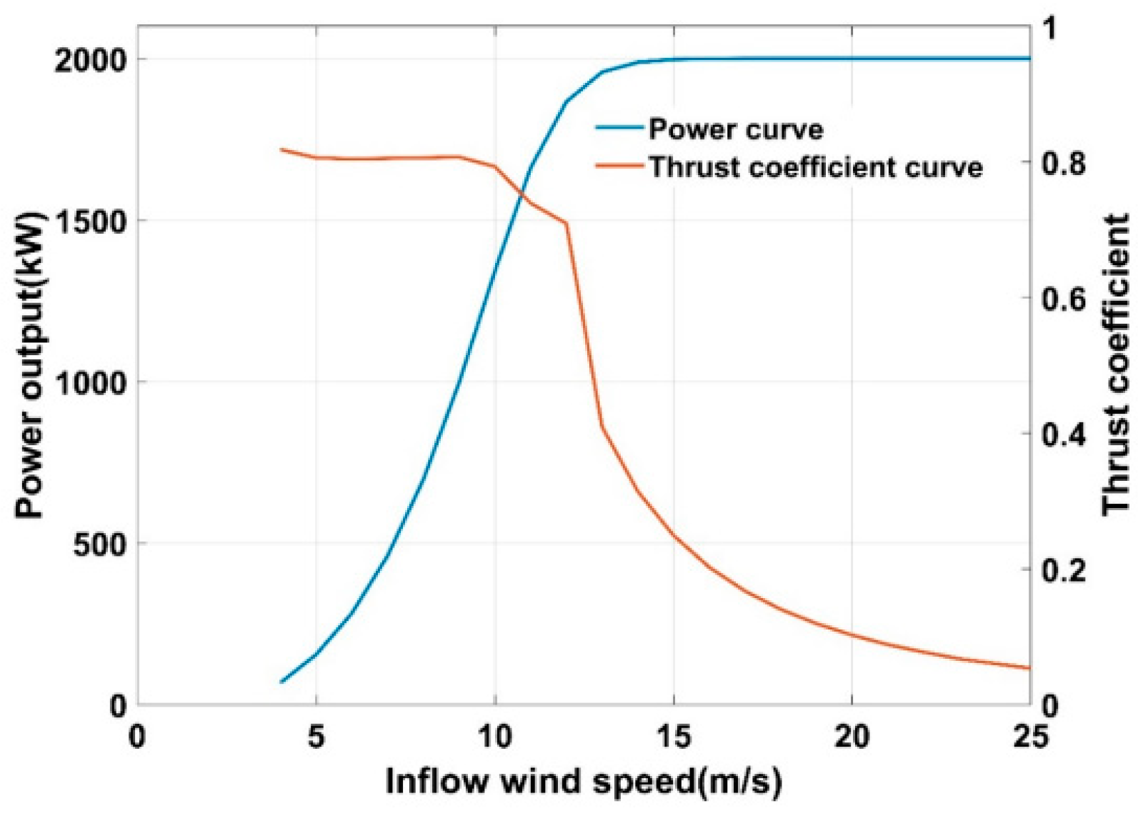
The Horns Rev wind farm is a large-scale offshore wind farm, which is often used for wake prediction studies around the world because of its long-term observation data. The wind farm consists of 80 Vestas-V80 2 MW wind turbines arranged in a regular array of 8 rows and 10 columns distanced by 7D. The Vestas-V80 2 MW wind turbine has a diameter of 80 m and a hub height of 70 m. The power curve and thrust coefficient curve of the wind turbine are shown in Figure 7.

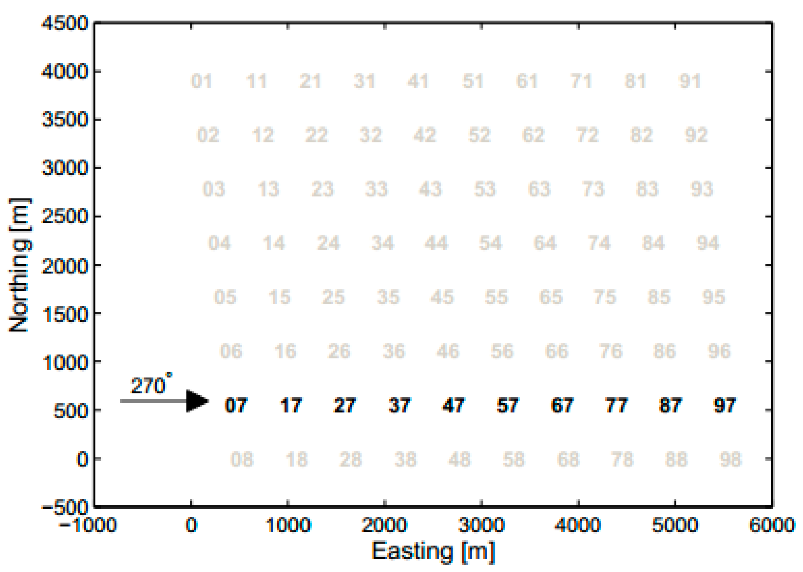
When the wind direction is westerly, that is, the incoming flow is 270°, the difference in the average power of rows 2~7 is negligible compared with that of rows 7 alone [34]. Therefore, as shown in Figure 8, the 10 wind turbines in the 7th row of the wind farm are used as the simulation objects to study wind farm wake regulation.

4.1. Simulation Settings

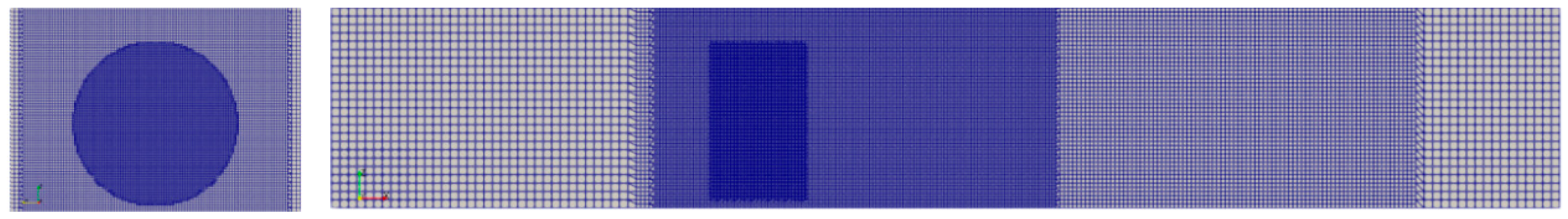
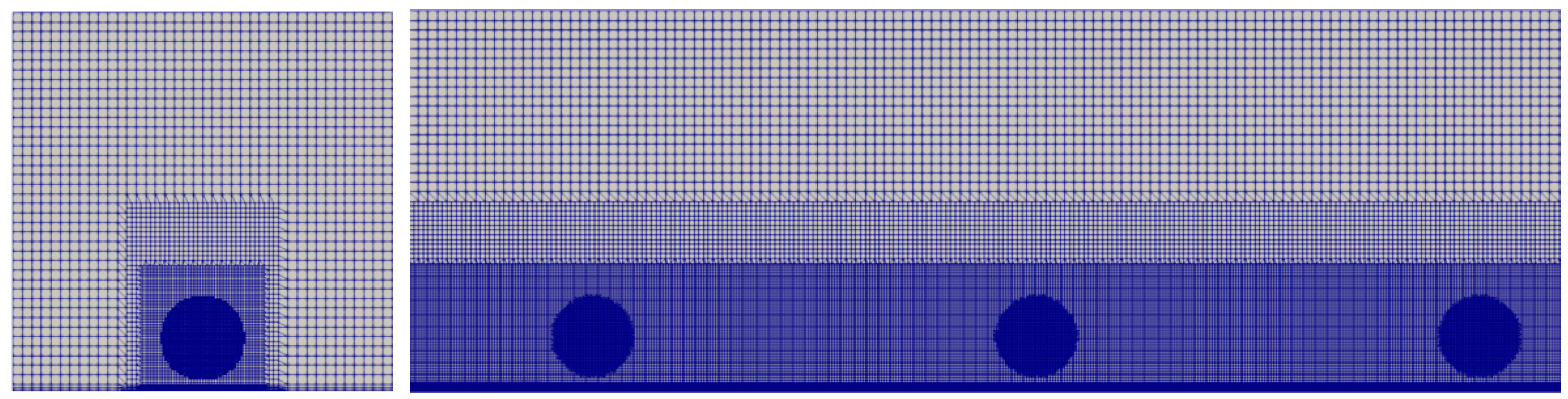
In the ALM method, the size of the calculation domain is set to 6240 m × 480 m × 480 m, that is, 78D × 6D × 6D. The first wind turbine is located downstream of the inlet surface, and the spacing of all wind turbines is 7D. Sarlak et al. [35] studied the effect of blockage rate on the simulation of wind turbine wake and the results show that when the blockage rate is greater than 5%, it will affect the simulation results of wind turbines, and the blockage rate is usually required to be less than 3%. The blockage rate of this case is 2.2%, which satisfies the corresponding requirements. The open-source structural mesh generator blockMesh is used to generate the background grid, and the snappyHexMesh is used for mesh refinement. The ALM mesh was refined three times, and the minimum mesh size after refinement was 1.5 m, which is less than 1.722 m, in compliance with the requirement that the mesh resolution is less than half of the maximum chord length of the blade [36]. The final mesh has about 13.02 million grid nodes, and the entire flow field consists of hexahedral cells, ensuring overall good mesh quality. The non-orthogonality, max aspect ratio, max skewness, and face pyramids are shown in

Table 1. Mesh quality parameters.

Elements	Result
Non-orthogonality	0 (ok)
Max skawness	6.8 × 10−13 (ok)
Face pyramids	ok
Max aspect ratio	1 (ok)

. Figure 9 shows a schematic diagram of the partial ALM mesh refinement, only three of the ALM zones are shown along direction.

Reynolds-averaged Navier–Stokes equations have been solved with an extended k-ε turbulence model. A velocity shear distribution in a logarithmic rate profile is set at the inlet of the domain. The wind speed at the hub height is 8.5 m/s, and the turbulence intensity is set at the magnitude of I = 8%. The outlet face boundary is set to the pressure outlet, the lower bottom boundary to the non-slip wall, and the upper and left and right boundaries to the slip boundary.

The simulation time step is set to 0.025 s, with a total simulation time of 2000 s, and the convergence residual is set to 10⁻⁶. The minimum mesh size is 1.5 m, and the flow velocity is 8.5 m/s. The calculated maximum CFL number is approximately 0.1417, which is less than 1, indicating a high level of computational stability.

For the wake model calculation, the open-source code, FLORIS, was used to simulate the wake flow, developed by the National Renewable Energy Laboratory (NREL). FLORIS is a low-cost, control-oriented modeling tool used for the calculation of steady-state tail current characteristics of wind farms, with a variety of built-in wake models and optimization algorithms available for a combination of choices, with the visual display of flow field, power generation assessment of wind farms, and optimization of tail current yaw control functions. It has the functions of flow field display, wind farm power generation assessment, wind farm turbine layout optimization, and wake yaw optimization control.

The execution process of yaw optimization firstly uses the velocity loss model, yaw wake model, and wake superposition model in the engineering wake model to describe the distribution of wake loss in the actual wind farm, the yaw wake offset of the yawing wind turbines, and the superposition of wake loss under the influence of upstream multiple wind turbines to achieve the functions of assessing the loss of the wake in the wind farm and the prediction of the output power; and secondly, takes the yaw angle of each unit as the optimization variable, and makes use of the intelligent optimization algorithm to establish a single-objective or multi-objective optimization algorithm. Secondly, the yaw angle of each unit is used as the optimization variable, and the intelligent optimization algorithm is used to establish a single-objective or multi-objective optimization module, which outputs the optimal yaw control strategy for wind farms under different wind conditions and arrangements.

The simulation adopts the BPA wake model and the Bastankhah yaw model built in FLORIS to describe the development of wake under the yaw condition of a single unit, establishes a fast calculation method for the wake of multiple wind turbines using the square and wake superposition model, and then uses the SciPy (Sequential Least Squares Programming)-based SciPy (Sequential Least Squares Programme) optimization controller for the maximum power generation of the whole farm. The optimization controller is used to perform the single-objective optimization calculation for the maximum power generation of the whole field. The main empirical parameter in the wake model, i.e., the wake expansion coefficient, is set to the value k* = 0.38 in reference [32], and the parameter is calibrated based on the Horns Rev I. wind farm example in the subsequent calculation work.

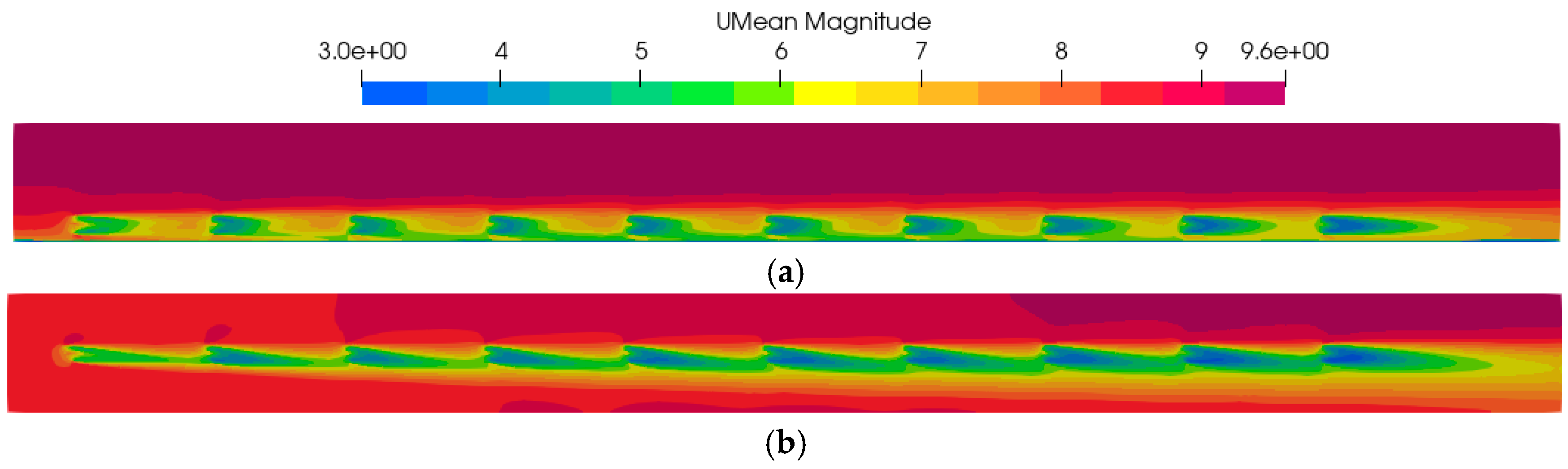
4.2. Without Wake Regulation

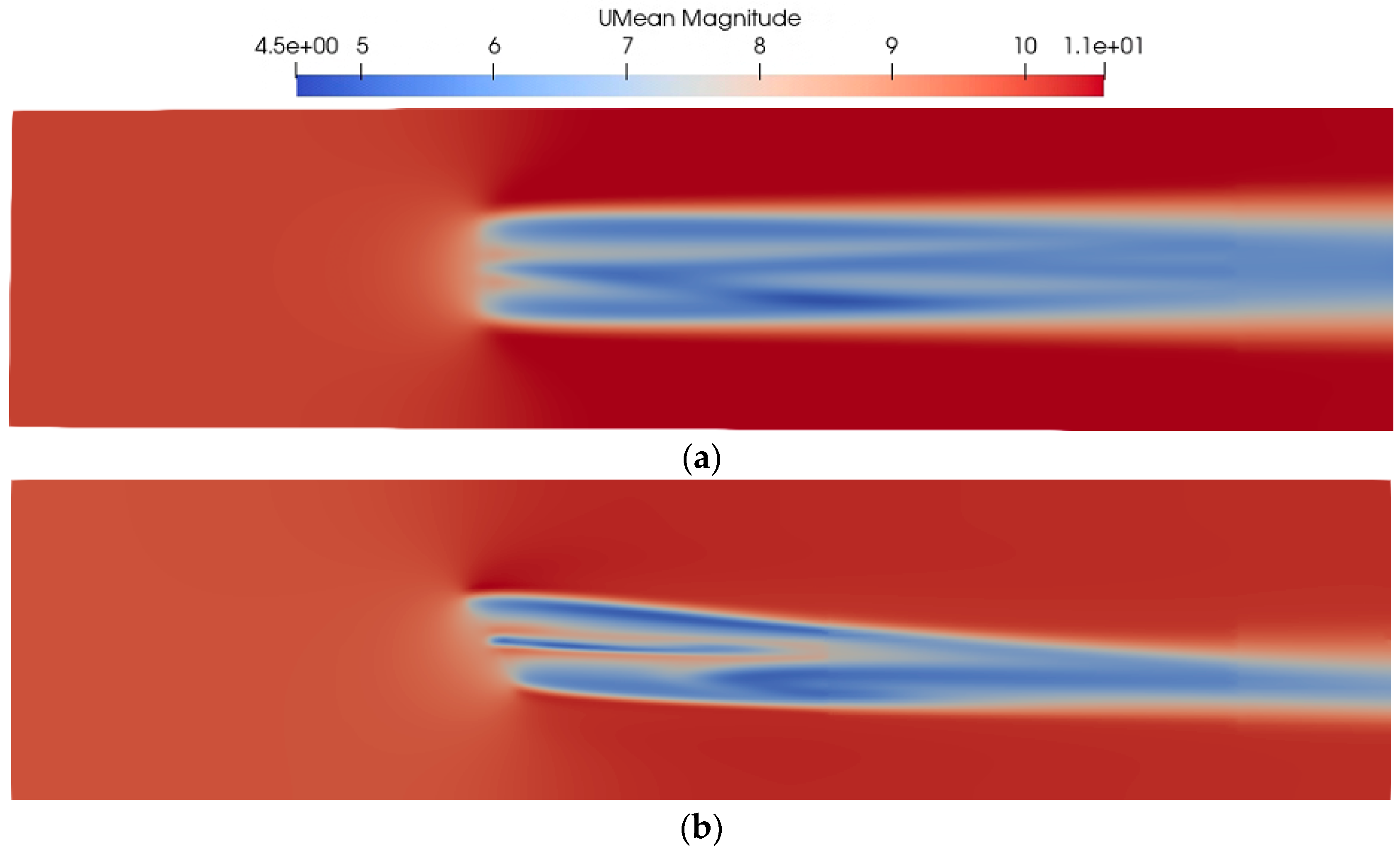
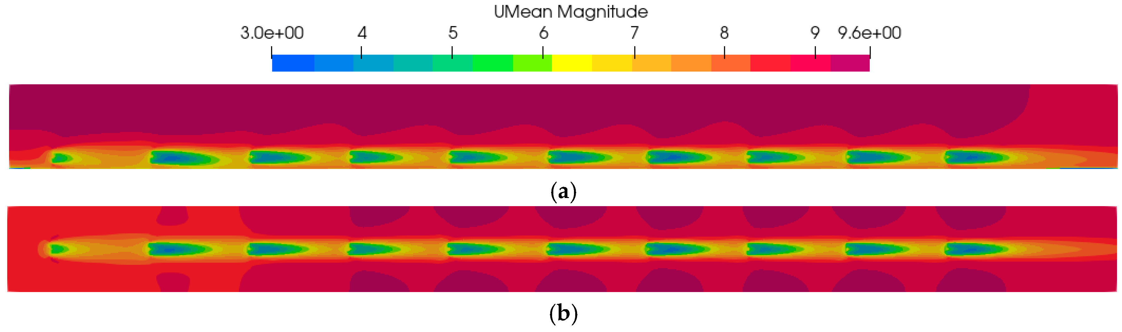
Figure 10 shows the velocity contour of the ALM simulated results at the hub height wind speed of 8.5 m/s. It can be seen from the results that the wind speed behind each wind turbine is the lowest, and gradually recovers with the increase in distance, and the wake can recover to about 7 m/s at about 5D downstream of each wind turbine. The expansion of the wake can be clearly seen from the horizontal velocity profile, and it is found that the shape and area of the wake low-speed area of the first wind turbine are the smallest, and the area of the low-speed area of the wake of the second wind turbine is slightly larger than that of the other wind turbines in the rear row.

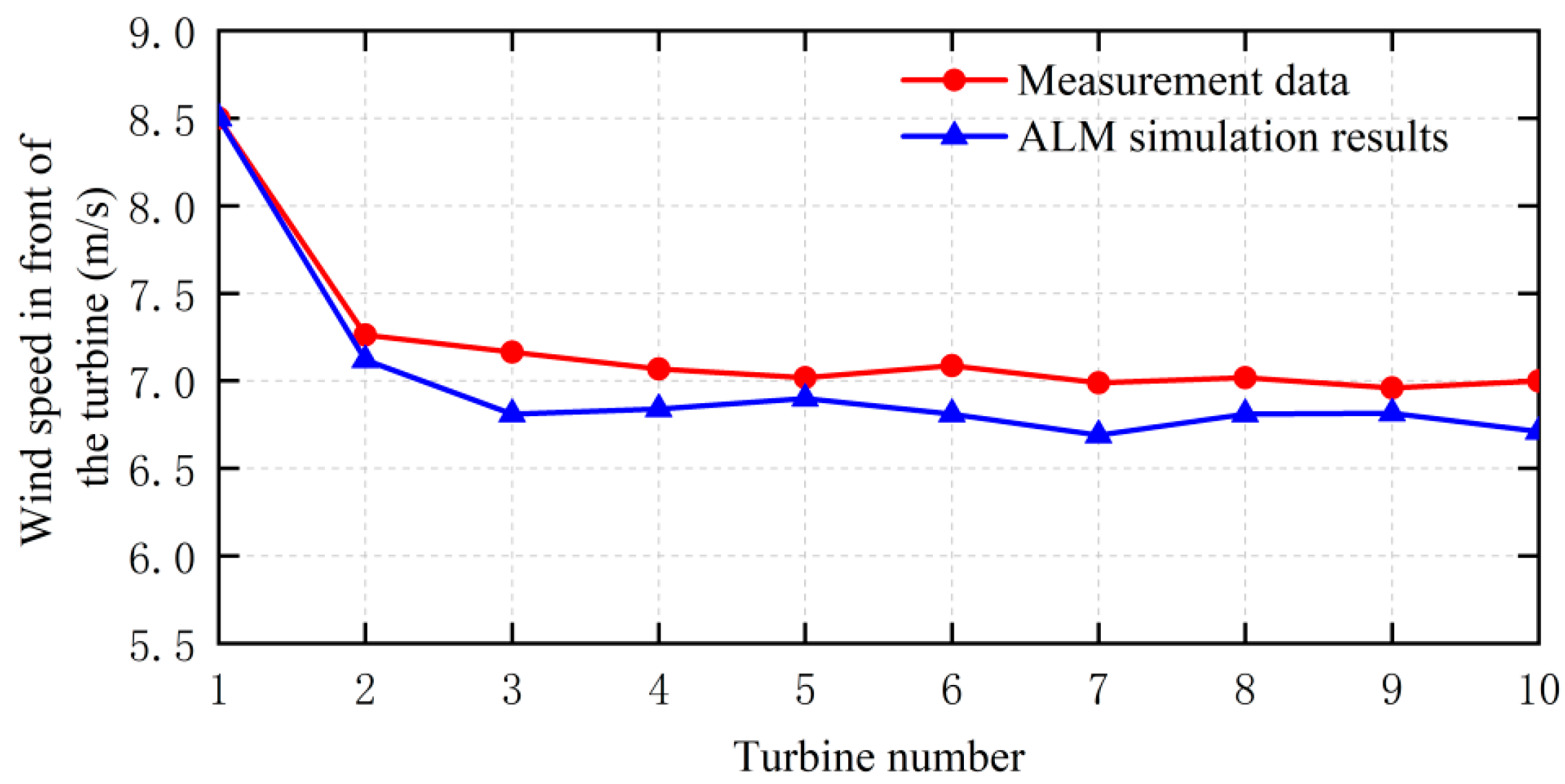
Figure 11 shows the comparison between the ALM simulation results and the measured wind speed data in front of each wind turbine in row 7 of the wind farm. It can be seen that the ALM simulation has satisfied agreement with the measurement data. The maximum relative error is about 4.4%, occurring at the third wind turbine. The relative error is defined by the absolute error normalized by the incoming wind speed, i.e., 8 m/s. It shows that the ALM can predict the recovery of wind speed in the wake of tandem wind turbines with high accuracy.

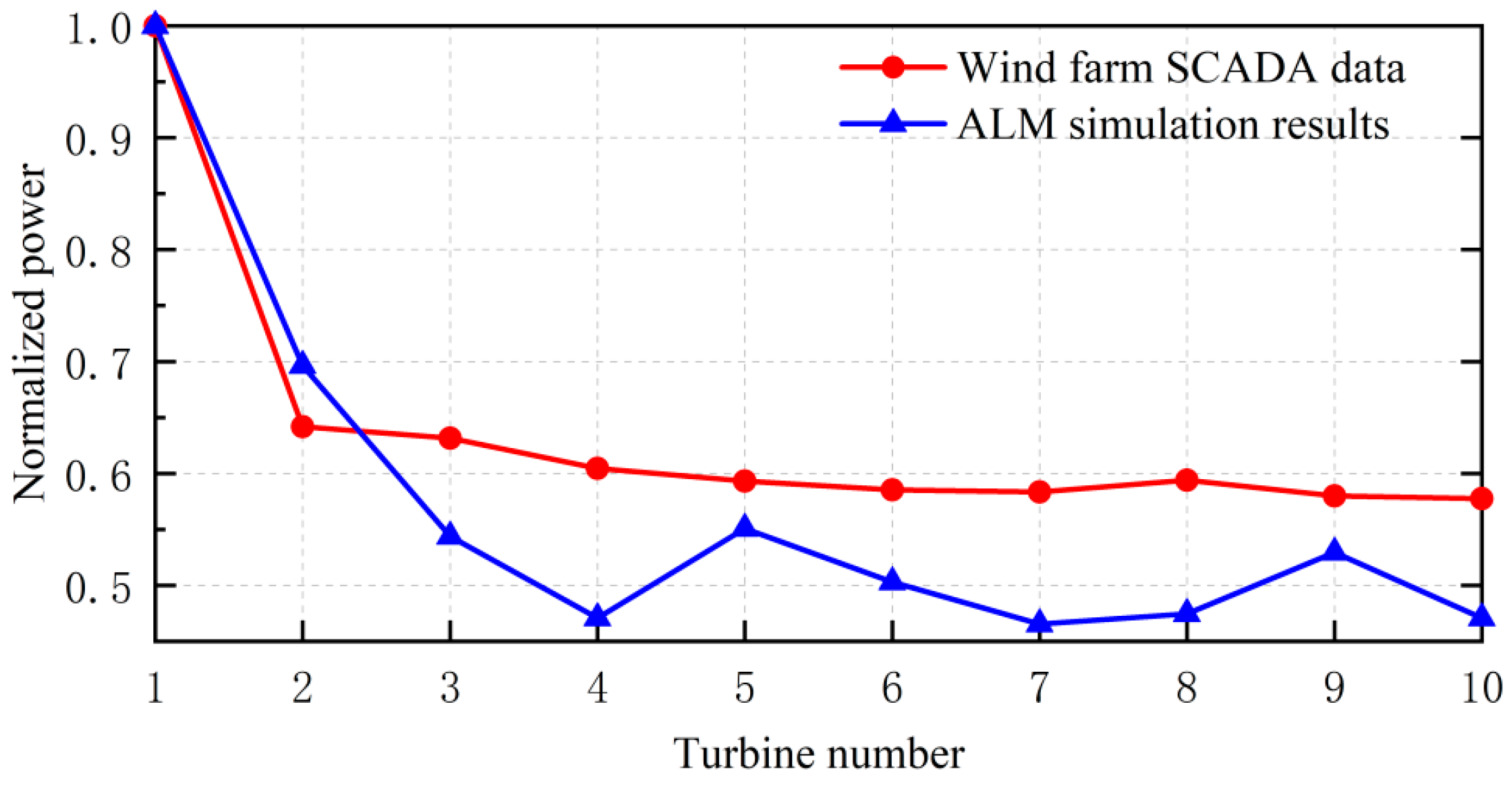
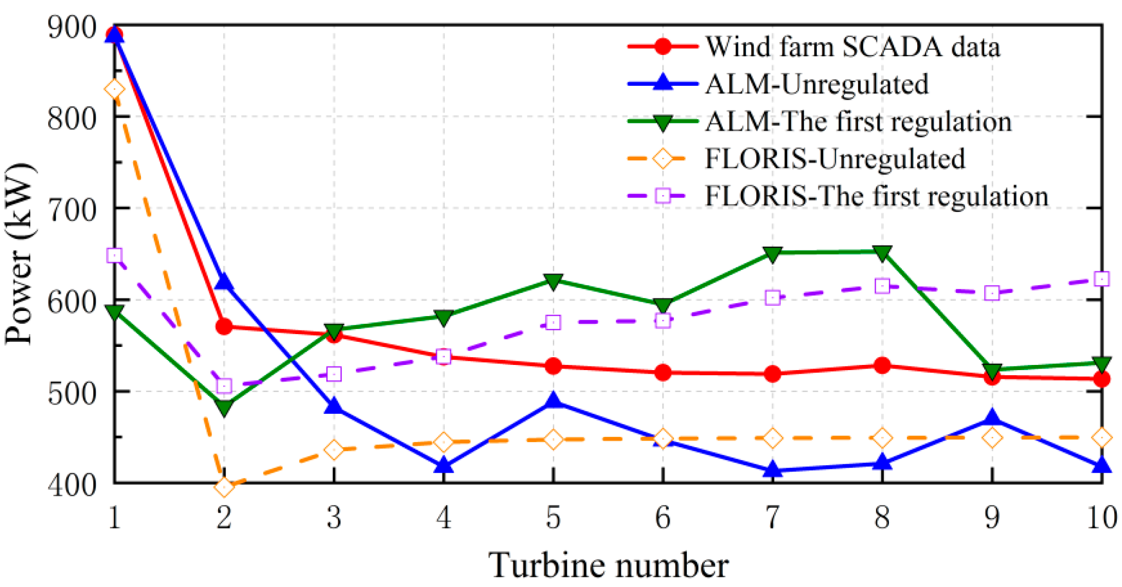
The calculation results of the ALM power are compared with the SCADA data of the wind farm, and the curves are shown in Figure 12. The SCADA data show that the power of the wind turbines from the 2nd to the 5th unit decreases one by one, and the power of the back row wind turbines is no longer decreasing and basically remains stable. The ALM successfully simulates the decreasing trend of the power of the back row wind turbines of the tandem wind turbines in the wind farm, but among them, the 5th and the 9th wind turbines have an increase in power compared to the previous one because of the sufficient turbulence in the wake stream and the exchange of kinetic energy. Following kinetic energy exchange, the wind speed has recovered, and the power has increased compared to the previous unit. Except for the first two wind turbines, the ALM simulated power output of the back-row wind turbines is overall lower than the measured data published by the wind farm, and the maximum deviation of power between the two is 11.9%, which occurs in the 8th turbine. Since the SCADA data are the averaged results over a period of time and the actuator line is difficult to accurately restore, the control law of the unit itself in the transient simulation leads to a certain degree of error in the calculation of the power coefficient Cp by the ALM. Considering that the power of the wind turbine is proportional to the cubic of the wind speed, it is still enough to consider that the ALM simulation of ten wind turbines established in this paper has high accuracy.

According to the wind farm SCADA data, the total power of the ten wind turbines in row 7 is calculated to be 5682.695 kW. The total power of the ten wind turbines simulated in this paper is 5061.183 kW, and the relation error is 10.94%, which can be considered to be within the allowable error range [5].

Similarly, the 10 wind turbines in line 7 of Horns Rev I. were modeled using the open-source wind farm wake control software FLORIS—3.5 to verify the accuracy of the wake disturbance simulation of the software.

Figure 13 shows the normalized power calculated by FLORIS, and it is observed that although the error of the second wind turbine reaches 16.56%, it can correctly simulate the trend of decreasing power of the tandem arrangement wind turbines. FLORIS calculates a total power of 4798.354 kW from the SCADA measurement, which is 15.56% off. Relevant studies have shown that due to the existence of more idealistic assumptions and empirical parameters in the derivation of the wake model, the recovery of the wake will be underestimated in the process of practical application, resulting in high results of the calculation of the wake loss [37]. The comprehensive comparison shows that the engineering wake model is lower than the ALM in the accuracy of wind farm total power prediction, and the use of ALM for correction has guiding significance.

4.3. Wake Regulation Without Parameter Calibration

The wake regulation without parameter calibration is performed first. The improved genetic algorithm is used to optimize the yaw angle in the wake regulation strategy. The maximum yaw angle change is set to ±30°, the wind turbine change in yaw angle was 0.25°, and the optimal yaw matrix of ten wind turbines in row 7 was obtained.

According to the yaw matrix calculated using FLORIS without parameter calibration, the yaw angle of each wind turbine was set separately for CFD-based ALM simulation, the yaw matrix shown in

Table 2. Yaw matrix without parameter calibration.

Index of Wind Turbine	1	2	3	4	5	6	7	8	9	10
Yaw angle/°	28.15	22.5	22.5	22.5	18.75	18.75	15	11.25	11.25	0

. The calculated wake velocity contour is shown in Figure 14. The cross-section of the deflection of the wake can be observed from the horizontal profile at the hub height. The first wind turbine has the largest yaw angle and the narrowest low-speed area of the wake; the second wind turbine realizes the deflection of the wake at a larger angle from the first wind turbine. Compared with Figure 9, it is seen that the rear wind turbine is reduced by the influence of the wake, and the area of the wind turbine obtains a relatively higher incoming wind speed.

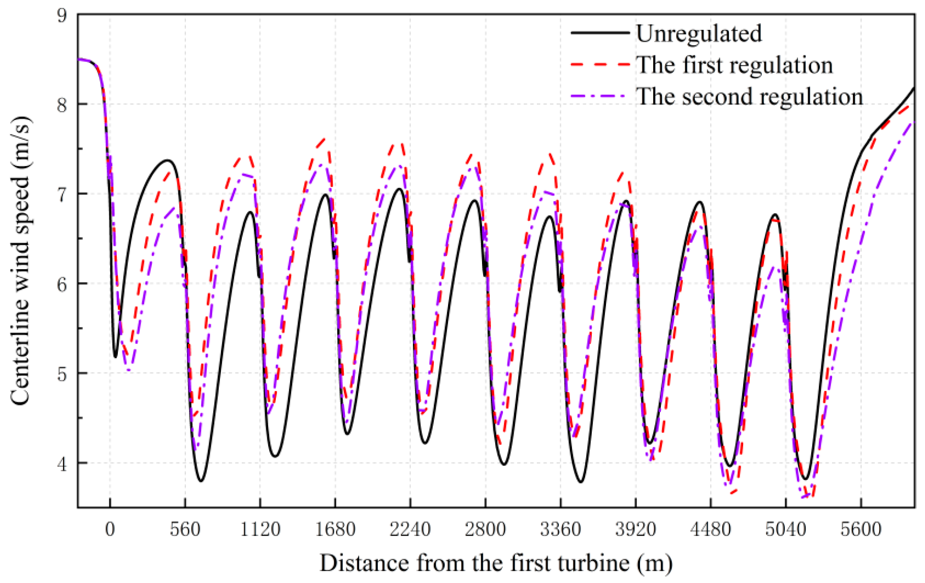
By extracting the wake velocity at the centerline of the contour map, shown in Figure 15, it can be found that before the implementation of the wake regulation, the inlet wind speed of the third wind turbine is lower than that of the second wind turbine, then increases slightly, then decreases in the 6th and 7th wind turbines, and then the inlet wind speed in front of the 8th wind turbine increases slightly. After the implementation of the active yaw control strategy, the incoming wind speed in front of the 3rd~8th wind turbines increased significantly due to the wake deflection of the upstream wind turbines.

The most direct test criterion for the implementation of active wake regulation is the increase in wind turbine power. It can be intuitively observed from the curve shown in Figure 16 that the power of the rear wind turbine is greatly increased after the implementation of active wake control. After active yaw control, the total power of the ten wind turbines was 5808.97 kW, which was 21.06% higher than that before the regulation. According to the calculation results of the ALM, the total power is 5794.65 kW, which is 14.49% higher than that before regulation.

4.4. Wake Regulation with Parameter Calibration

As shown in previous section, the wake model results have obvious differences to the ALM results. According to the wake expansion and deflection data obtained by the ALM results and the power calculation results, the parameter k* of the BPA model in FLORIS was corrected to 0.5. Then, adjusting the parameters of the engineering wake model in FLORIS, the updated yaw matrix is obtained as shown in

Table 3. Yaw matrix with twice parameter calibrations.

No. of Wind Turbine	1	2	3	4	5	6	7	8	9	10
Yaw angle/°	22.5	22.5	22.5	18.75	18.75	15	15	11.25	7.5	0

.

When k* is 0.5, the total power of the wind farm before the implementation of active wake regulation is 5388.04 kW, and the total power after the optimized control is 6050.38 kW, which is increased by 12.29%. The second CFD simulation is performed according to the updated yaw matrix.

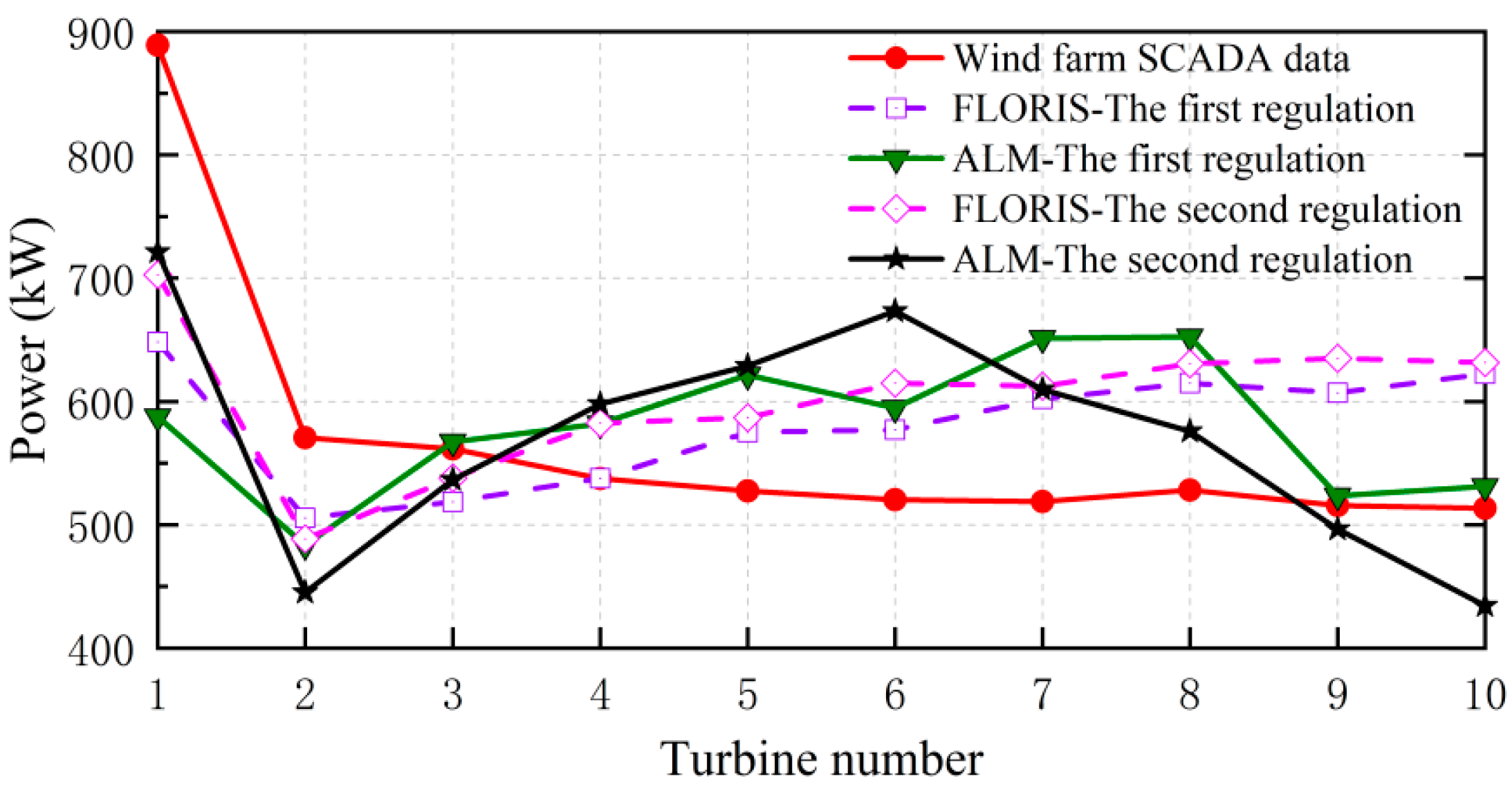
Figure 17 shows the change process of wind speed at the centerline of the horizontal profile of the hub height, and it is found that the highest point of the second simulated wake velocity recovery between the two wind turbines is lower than that of the first one, indicating that the overall recovery degree of wake is slightly weaker than that of the first iteration. The simulated power of each wind turbine is shown in Figure 18, and the power output of each wind turbine has some variations. For example, the power of the first wind turbine increases due to the decrease in its yaw angle, the second wind turbine is affected by the wake of the first wind turbine, the power decreases, and the power of the rear wind turbine gradually increases. The FLORIS simulation results show a steady increase in the rear wind turbines, while the CFD-based ALM simulation results show that the power decreases in the 6th and 8th wind turbines, respectively.

In

Table 4. The total power of the wind farm before and after the implementation of active wake regulation.

Working Conditions		Total Power Capacity/kW	Relative Increment
FLORIS, k* = 0.38	Non-yaw	4798.35	/
	Wake regulation with once parameter calibrations	5808.97	21.06%
FLORIS, k* = 0.5	Non-yaw	5388.04	/
	Wake regulation with twice parameter calibrations	6050.38	12.29%
ALM	Non-yaw	5061.18	/
	Wake regulation with once parameter calibrations	5794.65	14.49%
	Wake regulation with twice parameter calibrations	5719.90	13.02%

, the total power of the wind farm simulated by the ALM with the second active yaw control strategy is 5719.9 kW, which is 13.02% higher than that before yaw control. The second active yaw control strategy is 1.47% lower than the first strategy, because the yaw angle of the first wind turbine decreases and the yaw angle of other wind turbines changes, resulting in the wind speed of some wind turbines in the back row being lower than that of the first-time yaw strategy, so that the total power is slightly becoming lower.

In the process of the wake regulation for the first time in the previous section, k* = 0.38, and the difference between the ALM results and the wake model results is about 6.57%. Comparing the results of the second active yaw control strategy, the total power increase before and after yaw control was 13.02% and 12.29%, respectively, with a difference of only 0.73%. After two iterative calculations of wake control, the model parameters of the FLORIS software were successfully calibrated using the results of the CFD-based ALM simulation. It proved that the method proposed in this paper by using CFD-based ALM simulation and iterative calculation of engineering wake model can improve the credibility and implementability of the active wake control strategy of wind farms. It should be noted that the calibration could be iterated multiple times till an error tolerance is reached. For the current case, only two CFD-based ALM simulations were performed and, thus, the computational cost increase is neglectable.

Since the accuracy and reliability of the CFD-based ALM simulations and the wake model may have a large difference due to the changes in the application scenario, the actuator line model with less simplification has high confidence in the power calculation results. Moreover, the verification work of the exemplification carried out in this paper is sufficient to confirm the high accuracy of the ALM.

5. Conclusions

A parameter calibration method for the deflection engineering wake model by coupling the actuator line model was proposed in this paper. Based on this coupled method, an active yaw control of wind turbines was established and validated using the Horns Rev wind farm case. The following conclusions were obtained:

• CFD-based ALM simulation can correctly predict the recovery rate and deflection of the wake of wind turbines under different turbulence intensities. Especially in the case of large yaw angle, the prediction of the wake deflection angle of the ALM method has much better prediction compared to that of the wake model.
• Both the wake model and the ALM based on the engineering wake model can correctly simulate the change trend of the power decline of the rear wind turbine when the number of rows in the random group increases. However, for the prediction of the increase amplitude of the total power of the wind farm before and after yaw control, the empirical parameters of the engineering wake model using the default value may overestimate the increase in the total power.
• After calibrating the parameters of the wake model in the FLORIS software using the ALM simulation results, the gap between the two power predictions is greatly reduced. The effectiveness of the proposed wake regulation method coupling the actuator line model and the engineering wake model is proved, and the credibility of the prediction of the wake control effect of wind turbines is improved with only a small computational cost increase.

It should be noted that the main research objective of this paper is to establish a coupled approach of two wake simulation methods for wake regulation in wind farms. Only 2D wake models are used. In future work, 3D Gaussian wake models will also be considered for the research.