Improved Fault Detection Using Shifting Window Data Augmentation of Induction Motor Current Signals

Abstract

Deep learning models have demonstrated potential in Condition-Based Monitoring (CBM) for rotating machinery, such as induction motors (IMs). However, their performance is significantly influenced by the size of the training dataset and the way signals are presented to the model. When trained on segmented signals over a fixed period, the model’s accuracy can decline when tested on signals that differ from the training interval or are randomly sampled. Conversely, models utilizing data augmentation techniques exhibit better generalization to unseen conditions. This paper highlights the bias introduced by traditional training methods towards specific periodic waveform sampling and proposes a new method to augment phase current signals during training using a shifting window technique. This approach is considered as a practical approach for motor current augmentation and is shown to enhance classification accuracy and improved generalization when compared to existing techniques.

1. Introduction

The fourth industrial revolution, known as Industry 4.0, is transforming modern manufacturing through the development and integration of advanced technologies. This revolution is reshaping how companies manufacture, enhance, and distribute products. A key aspect of this industrial renaissance is the integration of new technologies, such as data-driven intelligent fault diagnosis. Early fault detection is essential in manufacturing to maintain reliability, where the continuous operation of equipment is imperative. Induction motors (IMs), being among the most vital equipment of the industrial sector [1], are a primary focus for Condition-Based Monitoring (CBM) in preventing expensive and unplanned downtimes [2].

Contemporary CBM strategies increasingly incorporate data-driven techniques, particularly machine learning (ML) methods, for fault detection of rotating machinery [3]. A key benefit of ML approaches is their independence from prior system knowledge, contrasted to traditional methods that required expert intervention and bespoke designs for each equipment. Additionally, ML methods are recognized for their robustness to varying operating conditions and parameter fluctuations, making them highly effective in challenging industrial environments. Numerous ML techniques have been proposed for fault diagnosis in IM applications including Deep Neural Networks [4], Radial Basis Functions [5], Auto-encoders [6,7,8,9], 1-D Convolutional Neural Networks [10,11], and 2-D Convolutional Neural Networks (CNN) [12,13,14,15,16,17,18,19,20,21,22,23]. Among the used deep learning architectures, the most used ones are CNN strategies. These models have been shown to provide higher classification accuracy when compared to other techniques. Particularly, 2-D CNNs are advantageous to 1-D strategies due to time–frequency analysis (TFA) techniques. For 2-D CNN applications, the waveform is directly transformed into time–frequency representations, known as a spectrogram, that captures both temporal and frequency information. Using local receptive fields, 2-D CNNs are adept at learning local hierarchical patterns, such as specific frequency bands at certain times. While using the original waveform preserves the temporal structure, it may not capture frequency information as effectively as a spectrogram.

Although current research shows that ML techniques perform well in fault classification of IMs, when preprocessing data for training samples, these approaches must account for the practical constraints of signal acquisition. Typically, research employs a straightforward signal segmentation technique for data preprocessing, where the signal is divided sequentially into equal-length segments [8,11,13,20,21,22,23,24]. Despite potentially achieving high accuracy during inference, this method lacks the robustness required for reliable deployment. Segmenting signals with periodic characteristics in this manner can cause signal characteristics to consistently appear in the same segment, leading the model to depend on these specific regions for fault discrimination. As a result, the model’s resilience and performance can deteriorate if the signal is not sampled at the same interval during field applications. Furthermore, CBM models require training on sufficiently large datasets to prevent overfitting and promote generalization [25]. Research has demonstrated that overlapping the segments can expand the training set [26,27]. However, a challenge with this method is determining the optimal overlap amount. Minimal overlap may lead to poor generalization, while excessive overlap can increase training times and strain memory resources.

In computer vision, data augmentation enhances the training dataset by artificially increasing the number and diversity of samples. Here, models are trained on these augmented images instead of the original ones. Common augmentation techniques include random cropping, scaling, contrast adjustments, and color jittering. These modifications are applied randomly with varying severity, ensuring that both augmented and original images are used during training. This study explores a data augmentation method that randomly crops the signal in every batch during training. The approach is applied to IM stator current signals for fault diagnosis and is compared to sequential segmentation and overlapping segmentation techniques. It is shown that when using the conventional slicing techniques, the model overfits to the training data which can result in the model becoming biased and ultimately reduces the performance of the model during practical implementation. Whereas the proposed shifting window data augmentation is demonstrated to have superior performance in terms of accuracy and generalization. The model is also shown to not have the bias observed with the conventional techniques.

2. Dataset and Methodology

2.1. Dataset

Electric machine faults, illustrated in Figure 1, are classified as either electrical or mechanical damage and can be further divided into stator, rotor, and bearing faults [3]. Bearing faults are the most common source of failure and are the most detrimental to the machine’s operation. The damaged bearing signals used in this study were obtained from the Kat-Data Center, contributed by the Mechanical Engineering Research Center at Paderborn University, Germany [28]. These data were collected from a 425 W motor, which has a nominal torque of T = 1.35 Nm, using thirty-two different ball bearings of type 6203. The ball bearings varied in condition, with 6 being healthy, 12 artificially damaged, and 14 subjected to accelerated lifetime damage. The test rig consisted of an IM, a torque-measurement shaft, a bearing module, a flywheel, and a load motor, as shown in Figure 2. A frequency inverter was used to operate the 425 W electric machine with a switching frequency of 16 kHz. The equipment used included a Type SD4CDu8S-009 from Hanning Elektro-Werke GmbH & Co. KG (Oerlinghausen, Germany) and a Combivert 07F5E 1D-2B0A from KEB Automation KG (Barntrup, Germany). The faults were tested multiple times under different operating conditions, as detailed in Table 1. The signals analyzed in this study were obtained from an IM with bearing damage, as shown in Table 2, operating under various conditions. For each bearing, 20 measurements were taken, each capturing 4 s of data. The signals were then filtered using a 25 kHz low-pass filter and sampled at a rate of 64 kHz.

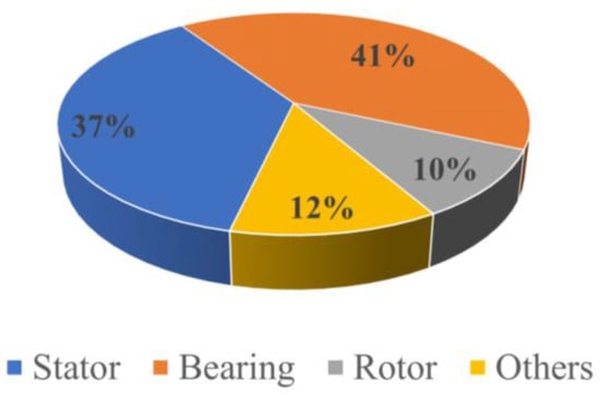
Figure 1. Percentage contribution of common IM faults.

Figure 2. Bearing test rig of Paderborn University experiment.

Table 1. Operating conditions of Paderborn University’s testbed.

Number	Rotational Speed [rpm]	Load Torque [Nm]	Radial Force [N]	Name of File
0	1500	0.7	1000	N15_M07_F10
1	1500	0.1	1000	N15_M01_F10
2	1500	0.7	400	N15_M07_F04

Table 2. Bearing damage files considered.

Bearing Damage	Bearing Codes	Class Label
Healthy Bearing	K001, K002, K003, K004, K005, K006	K0
Outer Ring	KA04, KA15, KA16, KA22, KA30	KA
Inner Ring	KI04, KI14, KI16, KI17, KI18, KI21	KI

2.2. Model

2.2.1. Convolutional Neural Network

The CNN is a fully connected, deep learning algorithm that combines feature extraction and feature classification approaches, particularly prevalent in the domain of computer vision. CNNs are structured with multiple convolutional layers, pooling layers, a fully connected layer, and a final output layer. Due to CNNs’ desirable features, such as local pattern extraction, translational invariance, and their ability to analyze frequency patterns across spectrogram representations [29], they have been shown to be adept in discriminating fault characteristics from IM signals. The classifier architecture adopted in this paper was taken from [30] and was considered for each test, as visually depicted in Figure 3.

Figure 3. Convolutional neural network model architecture.

The CNN model’s input layer takes a single spectrogram image with dimensions of 33 × 33. The initial convolutional layer uses 32 filters with a 5 × 5 kernel. Following this, a max-pooling layer is applied. The next two convolutional layers each use 32 filters with a 3 × 3 kernel, followed by another max-pooling layer. Subsequently, the final two convolutional layers each employ 64 filters with a 3 × 3 kernel, and another max-pooling layer is applied. All max-pooling layers use “same” padding and each have a size of 2 × 2. The outputs from these layers are flattened and connected to three fully connected dense layers with sizes 256, 1024, and 128, respectively. The Rectified Linear Unit (ReLU) activation function is applied to all layers due to its computational efficiency and reduced risk of gradient vanishing. The output layer uses a softmax activation function, with its size matching the number of classes within the dataset. The model architecture, along with the number of parameters, is detailed in Table 3.

Table 3. Structural parameters of the CNN model.

Layer	Output Shape	Parameter Numbers
Input	(None, 33, 33, 1)	0
Conv2d ((5, 5), 32)	(None, 29, 29, 32)	832
MaxPool2d (2, 2)	(None, 15, 15, 32)	0
Conv2d ((3, 3), 32)	(None, 13, 13, 32)	9248
Conv2d ((3, 3), 32)	(None, 11, 11, 32)	9248
MaxPool2d (2, 2)	(None, 6, 6, 32)	0
Conv2d ((3, 3), 64)	(None, 4, 4, 64)	18,496
Conv2d ((3, 3), 64)	(None, 2, 2, 64)	36,928
MaxPool2d (2, 2)	(None, 1, 1, 64)	0
Dense (256)	(None, 256)	16,640
Dense (1024)	(None, 1024)	263,168
Dense (128)	(None, 128)	131,200
Dense (3)	(None, 3)	387
Total Parameters:		486,147
Trainable Parameters:		486,147
Non-trainable Parameters:		0

The model for these trainings was constructed using Keras 2.10.0 on TensorFlow 2.10.1 and trained on a workstation with an Intel i9-13900K CPU, 64-GB main memory, and an NVIDIA GeForce 4090 GPU. During training, two callbacks were utilized: ReduceLROnPlateau and EarlyStopping. When a model’s Learning Rate (LR) is too large, the model can oscillate around the global minimum, approaching a sub-optimal solution. By tracking the model’s validation accuracy, the LR is decreased when the performance stagnates over four epochs by a factor of 2. EarlyStopping is a regularization strategy designed to avoid overfitting. This callback monitors for stagnation after a patience of ten epochs, where the training then terminates, potentially saving the model from overfitting.

2.2.2. Short-Time Fourier Transform

TFA technology finds broad applications in speech processing and equipment fault diagnosis [29,31]. Leveraging the feature extraction strengths of CNNs, TFA methods are employed to discern spectro-temporal patterns within signal waveforms to provide visual representations of spectrums for frequencies as they vary over time. Short-time Fourier transform (STFT) is one of the most frequently used time–frequency analysis methods. STFT is a modified Fourier transform that enables analysis of nonstationary signals in the time–frequency domain. STFT operates by dividing the time-domain signal into equally sized, localized windows and performs the Fourier transformation, thereby offering valuable time–frequency information while preserving locality in both axes of frequency and time. This enables the extraction of a frequency distribution within specific time intervals. In the realm of continuous-time analysis, the mathematical expression for STFT is as follows:

$$STFT\left(\tau ,\omega \right)={\int }_{-\infty }^{\infty }x\left(t\right)h\left(t-\tau \right)e^{-j\omega \tau }dt$$

(1)

where $h\left(t-\tau \right)$ denotes the window function centered at moment $\tau$, $\omega$ denotes the frequency, and $\tau$ indicates time. The magnitude squared of the STFT, known as a spectrogram, can then be used to approximate frequency components, constructed from (1) and (2), and is shown in Figure 4. Here, the horizontal and vertical axis represents time and frequency. The amplitude of a specific frequency at a given time is represented by the third dimension, color, where the dark blues correspond to low amplitudes and brighter colors to stronger amplitudes. Since the collected fault signals in rotating electric machinery are usually nonstationary [23], the STFT method is utilized in extracting the time–frequency-domain characteristics of the signals.

$$G\left(t,\omega \right)={\left|{\int }_{-\infty }^{\infty }x\left(t\right)h\left(t-\tau \right)e^{-j\omega \tau }dt\right|}^2$$

(2)

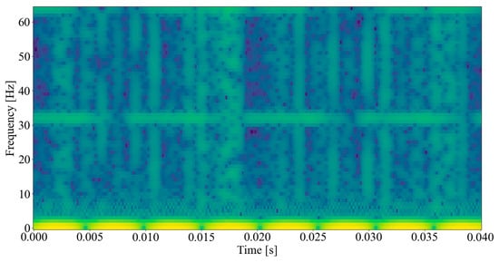
Figure 4. Spectrogram of phase current waveform.

2.3. Data Preprocessing

Data preprocessing involves formatting signals prior to their utilization in model training and testing. In motor current fault diagnosis, this process often involves segmenting the original signals into smaller, equally sized portions, thereby generating significantly sized datasets. These segments are subsequently randomized, then divided into training, validation, and testing samples for model training and inference. Depending on the model architecture, stator current samples may be utilized directly as time-domain signals [24] or transformed into time–frequency images using methods like STFT [31] or Continuous Wavelet Transform (CWT) [20]. Spectrograms can be generated either during the data preprocessing phase [15] or synchronously during training. For this study, the signal is segmented during the data preprocessing phase and is converted into a time–frequency image using STFT synchronously during training via the CPU.

Traditional Data Segmentation Techniques

When creating the segments for the dataset, strategies ordinarily employ sequential segmentation techniques, shown in Figure 5. Here, the original signal is partitioned into numerous smaller signals, each with $n$ data points. These segments are gathered sequentially, ensuring that every data point of the original signal is employed once.

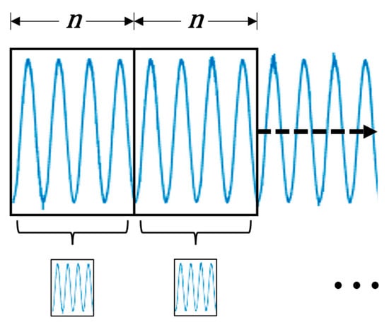
Figure 5. Traditional sequential segmentation preprocessing technique for motor current samples.

One concern with this approach is the potential repetition of fault characteristics within the signal, such as when the stator current aligns with the damaged bearing. In such cases, segments may contain fault information at distinct intervals. For instance, each signal within the depicted set consistently starts at the trough of the current waveform across the dataset, potentially biasing the model against samples lacking this feature. Additionally, Zhang et al. also suggest that this method overlooks the opportunity to generate more diverse samples for generalization [28]. Instead of shifting the next sample immediately after the previous one, as is traditionally performed, overlapping segments can be employed, as illustrated in Figure 6.

Figure 6. Overlapping segmentation preprocessing technique for motor current.

By overlapping the segments by $m$ data points, the signal is divided into more samples, with $m$ being smaller than $n$. This approach significantly expands the dataset, aiding in generalization. However, certain combinations of $n$ and $m$ may yield repetitive samples for the model. Still, there exists values of $n$ and $m$ that provide repeating samples for the model; thus, identifying optimal values of $m$ for effective model generalization can be time-consuming. Furthermore, because the dataset size is directly proportional to the value of $m$, using larger values of $m$ results in longer training times and can be challenging in terms of memory management.

In addition to sizing of the data samples, preprocessing strategies normalize the signals [12]. Normalization of signals is pivotal as it standardizes input features, facilitating quicker convergence during training. By constraining data within small intervals, near zero, the model mitigates overfitting risks and curbs issues such as exploding gradients. Additionally, this scaling further generalizes the model for all motor loads. In this study, the signals were each normalized by their $I_{RMS}$.

$$I={\displaystyle \frac{I_{MEAS}}{\sqrt{2}·I_{RMS}}}$$

(3)

where $I$ denotes the normalized sample, $I_{MEAS}$ is the measured current signal from the database, and $I_{RMS}$ indicates the calculated root mean square of the measured current signal.

2.4. Proposed Data Augmentation

Data augmentation involves artificially generating additional training data by applying random, yet realistic, transformations to existing samples. Unlike data preprocessing, which standardizes signals before training, data augmentation adjusts samples after each epoch with a certain probability. By integrating modified data, the model can learn from a broader and more varied dataset, enhancing its ability to generalize and perform well when faced with unseen samples. Without data augmentation, classification accuracy may seem to improve, but the model could practically struggle with performance across a wider range of samples. For this reason, we investigate the application of data augmentation and highlight its importance in the application of IM fault detection.

In the proposed data augmentation approach, the machine’s phase current signals are randomly modified during training. In the data preprocessing phase, we employ a similar slicing technique as demonstrated in the previous two methods, apart from using $N$ data samples rather than the previous $n$, where $N$ is a value larger than $n$. In each epoch, the data augmentation will impose random cropping of the sample to size it back down to $n$ data points through a shifting window operation, applicable to both sequential and overlapped segmented samples, as depicted in Figure 7a,b.

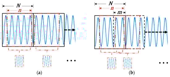
Figure 7. Shifting window data augmentation technique for motor current samples: (a) sequential segmentation and (b) overlapping segmentation.

The model is fed a more diverse and realistic dataset by applying random crops and shuffling the samples for each epoch. Thus, the samples will not begin at the same value for each epoch, allowing the model to ignore periodic characteristics, which is essential when considering practical implementations that do not have a meaningful way to capture signals at predetermined instances. Without zero-crossing detection, the signals collected from the field might not align with the intervals used during the preprocessing of training samples, potentially leading to reduced performance.

3. Results

3.1. Model and Training

The measured signal, $I_A$, was segmented into a sequence of frames consisting of an entire mechanical rotation of the electric machine. The number of samples required to represent a single revolution can be calculated from the following equations:

$$\mathrm{r}\mathrm{p}\mathrm{s}=\mathrm{r}\mathrm{p}\mathrm{m}/60$$

(4)

$$T_R={\mathrm{r}\mathrm{p}\mathrm{s}}^{-1}$$

(5)

$$s=f_{sampling}\times T_R.$$

(6)

where $s$ represents the data points completing one revolution, $T_R$ is the time required for one rotation, and $f_{sampling}$ is the sampling frequency. Thus, when the speed of the motor is $1500 \mathrm{r}\mathrm{p}\mathrm{m}$ and the sampling frequency is $64 \mathrm{k}\mathrm{H}\mathrm{z}$, (4)–(6) are calculated as follows: $\mathrm{r}\mathrm{p}\mathrm{s}=25$; $T_R=0.04$; and $s=2560$. A summarized flowchart of the shifting window procedure is shown in the flowchart in Figure 8. Here, the preprocessing was performed before the training, and the data augmentation was executed every epoch by the CPU to prefetch the samples to be used by the GPU for training in the next epoch.

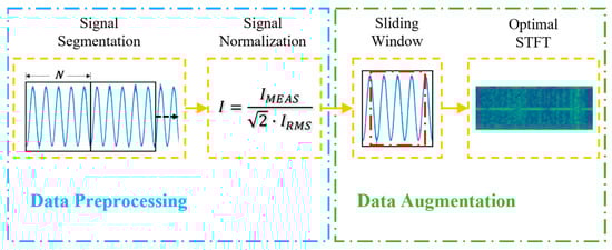
Figure 8. Flowchart of the proposed preprocessing and augmentation techniques.

3.2. Simulation Results

3.2.1. Random Sampling Test

For data preprocessing segmentation, $n$ was taken to be the same as $s$. The original signal was then divided in half, where the first half is preprocessed into the training data for each technique. To facilitate the shifting window data augmentation, the signals length for data augmentation tests were increased by 25%, providing $N=3200$. Similarly, for the overlapping signals, a value of $m=640$ was used, giving an overlapping of 25% between samples. The sizes of the resulting datasets, created by each technique, are provided in Table 4.

Table 4. Number of samples in each dataset.

Training Technique	Total Samples
Sequential segmentation	60,294
Shifting window with sequential segmentation	48,022
Overlapping segmentation	80,736
Shifting window with overlapping segmentation	64,384

Although the shifting window method has fewer samples for training, the data augmentation procedure will artificially increase the total number of samples observed by the model. The second half of the signals were then randomly sampled at $n=2560$, unmodified further into 51,000 unique samples, and were used to evaluate each method. The training samples were then randomly shuffled into an 80/20 testing/validation split. To evaluate the performance of these methods, all models were trained multiple times while varying hyper-parameters such as batch size and LR. After various trainings, the highest classification accuracy parameters were determined, as presented in Table 5.

Table 5. Benchmark model parameter settings.

Parameter	Setting
STFT Frame Length	100
STFT Frame Step	10
STFT Window	Hann
Batch Size	32
Initial LR	0.001
LR Factor	0.5
Optimizer	Adam
Loss Function	Categorical Cross-Entropy
Train/Val	0.8/0.2

The procedure was repeated ten times using these hyperparameters to obtain statistical characteristics. The accuracy and loss curves of the best-performing models from each method are compared in Figure 9 and Figure 10. Figure 11 and Figure 12 exhibit the confusion matrices for the trials without and with the proposed data segmentation, with predicted fault labels on the vertical axis and ground truth labels on the horizontal axis. The F1-score, recall, precision, and accuracy for these evaluations are detailed in Table 6, Table 7, Table 8 and Table 9. Figure 13 presents the box and whisker plot analysis of each strategy.

Figure 9. Model accuracy in the CNN training.

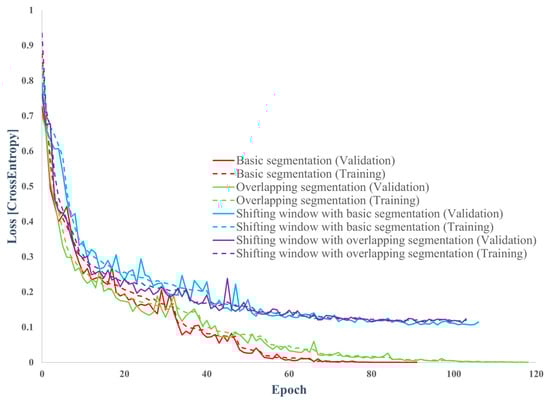
Figure 10. Cross-entropy losses in CNN training.

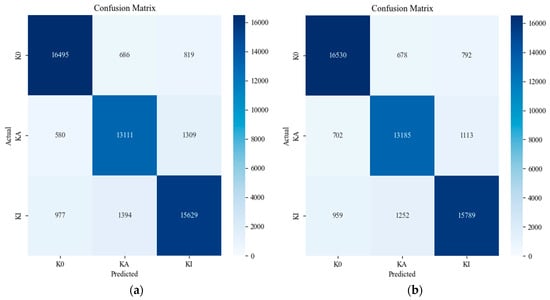
Figure 11. Confusion matrix for traditional segmentation techniques: (a) sequential segmentation and (b) overlapping segmentation.

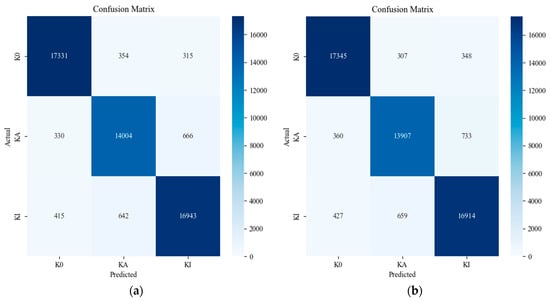
Figure 12. Confusion matrix for segmentation techniques using shifting window augmentation: (a) sequential segmentation and (b) overlapping segmentation.

Table 6. Analysis of sequential segmentation.

	Precision	Recall	F1-Score	Support
K0	0.9137	0.9164	0.9151	18,000
KA	0.8631	0.8741	0.8685	15,000
KI	0.8802	0.8683	0.8742	18,000
Accuracy			0.8870

Table 7. Analysis of overlapping segmentation.

	Precision	Recall	F1-Score	Support
K0	0.9087	0.9183	0.9135	18,000
KA	0.8723	0.8790	0.8756	15,000
KI	0.8923	0.8772	0.8847	18,000
Accuracy			0.8922

Table 8. Analysis of the shifting window with sequential segmentation.

	Precision	Recall	F1-Score	Support
K0	0.9588	0.9628	0.9608	18,000
KA	0.9336	0.9336	0.9336	15,000
KI	0.9453	0.9413	0.9433	18,000
Accuracy			0.9466

Table 9. Analysis of the shifting window with overlapping segmentation.

	Precision	Recall	F1-Score	Support
K0	0.9566	0.9636	0.9601	18,000
KA	0.9351	0.9271	0.9311	15,000
KI	0.9399	0.9397	0.9398	18,000
Accuracy			0.9444

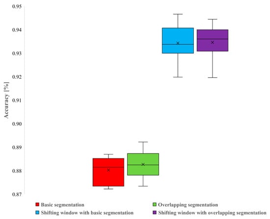
Figure 13. Model accuracy of each technique for all runs.

3.2.2. Predetermined Sampling Test

To further assess the impact of signal segmentation on model performance, a worst-case scenario is examined. In this scenario, the model is trained on segmented signals where each class starts at unique, predetermined intervals. During preprocessing, the original waveforms are time-shifted and segmented into 2560 datapoints across the entire signal. Specifically, K0 is time-shifted to its zero-crossing point; KA is time-shifted 160 datapoints past its zero-crossing point to start at a positive value; KI is time-shifted 320 datapoints past its zero-crossing point to start at a negative value. These signals are then partitioned into training and validation datasets, using an 80/20 split. For the testing dataset, a similar procedure is followed, but with different starting points for each class. KI is time-shifted to its zero-crossing; K0 is time-shifted 160 datapoints past its zero-crossing; and KA is time-shifted 320 datapoints past its zero-crossing. Figure 14 illustrates the resulting training and testing signals used. It is important to note that the training and testing datasets are identical, except for the intervals from which the segments are sampled from. Additionally, the testing dataset signals are specifically shifted, respective to the training data, to resemble that of a different class. Figure 15 and Figure 16 and Table 10 show the epoch metrics, confusion matrix, and statistical analysis, respectively, of the model trained with sequential segmentation tested on signals that were sampled at predetermined intervals.

Figure 14. Training and testing signals segmented around their zero-crossing for sequential segmentation.

Figure 15. Epoch metrics for model trained with sequential segmentation, sampled at predetermined intervals: (a) accuracy and (b) cross-entropy losses.

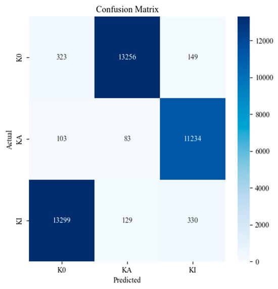
Figure 16. Confusion matrix for model trained with sequential segmentation, sampled at predetermined intervals.

Table 10. Analysis of model trained with sequential segmentation, sampled at predetermined intervals.

	Precision	Recall	F1-Score	Support
K0	0.0235	0.0235	0.0235	13,728
KA	0.0062	0.0073	0.0067	11,420
KI	0.0282	0.0240	0.0259	13,758
Accuracy			0.0189

To assess the efficacy of the proposed data augmentation method, we conducted the same test on a model trained using shifting window augmentation. The testing database was kept consistent with the previous procedure; while the training and validation datasets were generated using the same zero-crossing and time-shifting scheme, the signal lengths were extended from 2560 datapoints to 3200, resulting in a 25% overlap. Figure 17 displays the training signals used in this evaluation.

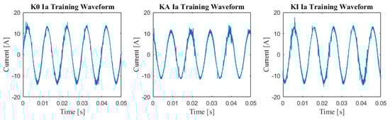
Figure 17. Training signals segmented around their zero-crossing for overlapping segmentation using shifting window augmentation.

Similarly, Figure 18 and Figure 19 display the epoch metrics and confusion matrix of the model trained using shifting window augmentation tested on signals that were sampled at predetermined intervals, respectively. Table 11 presents this model’s statistical analysis.

Figure 18. Epoch metrics for model trained using shifting window augmentation, sampled at predetermined intervals: (a) accuracy and (b) cross-entropy losses.

Figure 19. Confusion matrix for model trained using shifting window augmentation, sampled at predetermined intervals.

Table 11. Analysis of model trained using shifting window augmentation, sampled at predetermined intervals.

	Precision	Recall	F1-Score	Support
K0	0.9538	0.9663	0.9600	13,728
KA	0.9400	0.9321	0.9360	11,420
KI	0.9455	0.9396	0.9425	13,758
Accuracy			0.9468

To further underscore the impact of signal segmentation on model accuracy, a second type of machine learning model was included in this study. A recurrent neural network, specifically a Long Short-Term Memory (LSTM) model, was trained with the same procedures to verify whether the worst-case scenario had a meaningful impact on this type of model’s performance, as it had with the CNN model. Details of the LSTM model’s architecture and parameters are provided in Table 12.

Table 12. Structural parameters of the LSTM model.

Layer	Output Shape	Parameter Numbers
LSTM (128, (247,65))	(None, 128)	99,328
Dropout (0.2)	(None, 128)	0
Dense (128)	(None, 128)	16,512
Dense (64)	(None, 64)	8256
Dropout (0.4)	(None, 64)	0
Dense (48)	(None, 48)	3120
Dropout (0.4)	(None, 48)	0
Dense (3)	(None, 3)	147
Total Parameters:		127,363
Trainable Parameters:		127,363
Non-trainable Parameters:		0

Figure 20 and Figure 21 display the epoch metrics of the LSTM model trained using sequential segmentation and shifting window augmentation, respectively. Finally, Figure 22 demonstrates the confusion matrices for both these strategies.

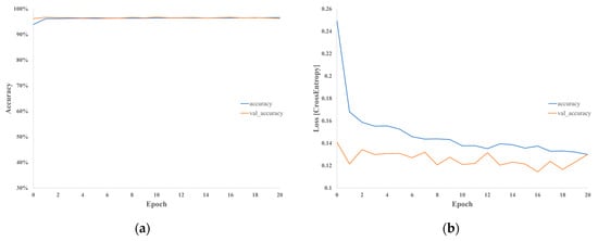
Figure 20. Epoch metrics for LSTM model trained using sequential segmentation, sampled at predetermined intervals: (a) accuracy and (b) cross-entropy losses.

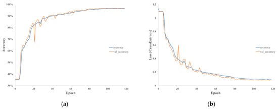
Figure 21. Epoch metrics for LSTM model trained using shifting window augmentation, sampled at predetermined intervals: (a) accuracy and (b) cross-entropy losses.

Figure 22. Confusion Matrix for LSTM model trained with samples at predetermined intervals using: (a) sequential segmentation and (b) shifting window augmentation.

4. Discussion

The model training curves suggest that models without augmentation clustered the training data more effectively. However, when evaluating the models on the random test samples, statistical analyses indicate that augmentation methods significantly improved performance. While models without data augmentation achieved near-perfect classification during training and validation, their maximum overall accuracy on unseen data was only 89.22%, indicating overfitting. In contrast, models with data augmentation maintained consistent accuracy across training, validation, and inference.

Across all trials, the models trained with data augmentation consistently outperformed when evaluating the randomly sampled datasets. Data augmentation improved accuracy by about 5.299% on average. Notably, when the testing data are segmented using the sequential segmentation technique, all models achieved over 99% accuracy. Additionally, when comparing the shifting window technique with sequential segmentation and 25% overlapping segmentation, it is observed that there was no appreciable gain in accuracy. These results indicate that the data augmentation procedure enhances the model’s ability to generalize for fault classification of IMs’ phase current signals, while also reducing the number of samples needed in the dataset.

Analyzing the epoch metrics, confusion matrix, and statistical analysis for the model trained with sequential segmentation and tested on time-shifted datasets reveals that data segmentation impacts overfitting. Despite being tested on the same waveforms used for training, the model’s performance significantly declined. During training, the model indicates high accuracy; however, it frequently misclassified K0 signals as KA, KA signals as KI, and KI signals as K0 during testing. This pattern mirrors the shifts in the training data, suggesting that the model developed a bias based on the signal presentation during training. In contrast, the model trained using shifting window augmentation showed time invariance in the presentation of testing signals, as indicated by the epoch metrics, confusion matrix, and statistical analysis. This overfitting issue in traditional sequential segmentation is evident in both CNN and LSTM models and is shown to negatively impact both models’ performance. This suggests that the preprocessing segmentation technique can degrade accuracy, regardless of the model topology used. Consequently, data augmentation proves to be an effective approach to realizing higher model generalization and accuracy for practical CBM applications.

5. Conclusions

This paper proposed a data augmentation framework for induction motors. In this approach, phase current samples from an IM, with varying degrees of bearing damage, were randomly cropped using a shifting window every epoch, enhancing database diversity while reducing its overall size. A convolutional neural network was employed as the deep learning model to automatically learn discriminative features of IM faults, with comparisons made between strategies with and without data augmentation. This study demonstrates that data augmentation improves the model’s generalizability, while models without augmentation tend to overfit. This improvement is crucial for practical applications, where it is not always possible to ensure that input data are referenced at the same point as the training data or that fault characteristics are in the same region. Future research could explore the accuracy of models using vibration data as input and investigate other advanced data augmentation techniques.

References

- Brusamarello, B.; da Silva, J.C.C.; Sousa, K.d.M.; Guarneri, G.A. Bearing Fault Detection in Three-Phase Induction Motors Using Support Vector Machine and Fiber Bragg Grating. IEEE Sens. J. 2023, 23, 4413–4421. [Google Scholar] [CrossRef]
- Liu, Y.; Bazzi, A.M. A review and comparison of fault detection and diagnosis methods for squirrel-cage induction motors: State of the art. ISA Trans. 2017, 70, 400–409. [Google Scholar] [CrossRef] [PubMed]
- Yakhni, M.F.; Cauet, S.; Sakout, A.; Assoum, H.; Etien, E.; Rambault, L.; El-Gohary, M. Variable speed induction motors’ fault detection based on transient motor current signatures analysis: A review. Mech. Syst. Signal Process. 2023, 184, 109737. [Google Scholar] [CrossRef]
- Afrasiabi, S.; Afrasiabi, M.; Parang, B.; Mohammadi, M. Real-Time Bearing Fault Diagnosis of Induction Motors with Accelerated Deep Learning Approach. In Proceedings of the 2019 10th International Power Electronics, Drive Systems and Technologies Conference (PEDSTC), Shiraz, Iran, 12–14 February 2019. [Google Scholar]
- Chattopadhyay, P.; Saha, N.; Delpha, C.; Sil, J. Deep Learning in Fault Diagnosis of Induction Motor Drives. In Proceedings of the 2018 Prognostics and System Health Management Conference (PHM-Chongqing), Chongqing, China, 26–28 October 2018. [Google Scholar]
- Li, C.; Zhang, W.; Peng, G.; Liu, S. Bearing Fault Diagnosis Using Fully-Connected Winner-Take-All Autoencoder. IEEE Access 2018, 6, 6103–6115. [Google Scholar] [CrossRef]
- Principi, E.; Rossetti, D.; Squartini, S.; Piazza, F. Unsupervised electric motor fault detection by using deep autoencoders. IEEE/CAA J. Autom. Sin. 2019, 6, 441–451. [Google Scholar] [CrossRef]
- Toma, R.N.; Piltan, F.; Kim, J.-M. A Deep Autoencoder-Based Convolution Neural Network Framework for Bearing Fault Classification in Induction Motors. Sensors 2021, 21, 8453. [Google Scholar] [CrossRef] [PubMed]
- Abdellatif, S.; Aissa, C.; Hamou, A.A.; Chawki, S.; Oussama, B.S. A Deep Learning Based on Sparse Auto-Encoder with MCSA for Broken Rotor Bar Fault Detection and Diagnosis. In Proceedings of the 2018 International Conference on Electrical Sciences and Technologies in Maghreb, Algiers, Algeria, 29–31 October 2018. [Google Scholar]
- Ince, T.; Kiranyaz, S.; Eren, L.; Askar, M.; Gabbouj, M. Real-Time Motor Fault Detection by 1-D Convolutional Neural Networks. IEEE Trans. Ind. Electron. 2016, 63, 7067–7075. [Google Scholar] [CrossRef]
- Gu, Y.; Zhang, Y.; Yang, M.; Li, C. Motor On-Line Fault Diagnosis Method Research Based on 1D-CNN and Multi-Sensor Information. Appl. Sci. 2023, 13, 4192. [Google Scholar] [CrossRef]
- Skowron, M.; Orlowska-Kowalska, T.; Wolkiewicz, M.; Kowalski, C.T. Convolutional Neural Network-Based Stator Current Data-Driven Incipient Stator Fault Diagnosis of Inverter-Fed Induction Motor. Energies 2020, 13, 1475. [Google Scholar] [CrossRef]
- Hsueh, Y.-M.; Ittangihal, V.R.; Wu, W.-B.; Chang, H.-C.; Kuo, C.-C. Fault Diagnosis System for Induction Motors by CNN Using Empirical Wavelet Transform. Symmetry 2019, 11, 1212. [Google Scholar] [CrossRef]
- Xu, G.; Liu, M.; Jiang, Z.; Söffker, D.; Shen, W. Bearing Fault Diagnosis Method Based on Deep Convolutional Neural Network and Random Forest Ensemble Learning. Sensors 2019, 19, 1088. [Google Scholar] [CrossRef]
- Du, Y.; Wang, A.; Wang, S.; He, B.; Meng, G. Fault Diagnosis under Variable Working Conditions Based on STFT and Transfer Deep Residual Network. Shock. Vib. 2020, 2020, 1–18. [Google Scholar] [CrossRef]
- Shao, S.; McAleer, S.; Yan, R.; Baldi, P. Highly Accurate Machine Fault Diagnosis Using Deep Transfer Learning. IEEE Trans. Ind. Inform. 2019, 15, 2446–2455. [Google Scholar] [CrossRef]
- Xu, G.; Liu, M.; Jiang, Z.; Shen, W.; Huang, C. Online Fault Diagnosis Method Based on Transfer Convolutional Neural Networks. IEEE Trans. Instrum. Meas. 2020, 69, 509–520. [Google Scholar] [CrossRef]
- Ibrahim, A.; Anayi, F.; Packianather, M. New Transfer Learning Approach Based on a CNN for Fault Diagnosis. In Proceedings of the 1st International Electronic Conference on Machines and Applications, Online, 15–30 September 2022. [Google Scholar]
- Zhong, H.; Yu, S.; Trinh, H.; Lv, Y.; Yuan, R.; Wang, Y. Fine-tuning transfer learning based on DCGAN integrated with self-attention and spectral normalization for bearing fault diagnosis. Measurement 2023, 210, 112421. [Google Scholar] [CrossRef]
- Chang, H.-C.; Wang, Y.-C.; Shih, Y.-Y.; Kuo, C.-C. Fault Diagnosis of Induction Motors with Imbalanced Data Using Deep Convolutional Generative Adversarial Network. Appl. Sci. 2022, 12, 4080. [Google Scholar] [CrossRef]
- Misra, S.; Kumar, S.; Sayyad, S.; Bongale, A.; Jadhav, P.; Kotecha, K.; Abraham, A.; Gabralla, L.A. Fault Detection in Induction Motor Using Time Domain and Spectral Imaging-Based Transfer Learning Approach on Vibration Data. Sensors 2022, 22, 8210. [Google Scholar] [CrossRef]
- Zhang, W.; Li, C.; Peng, G.; Chen, Y.; Zhang, Z. A deep convolutional neural network with new training methods for bearing fault diagnosis under noisy environment and different working load. Mech. Syst. Signal Process. 2018, 100, 439–453. [Google Scholar] [CrossRef]
- Xue, Y.; Yang, R.; Chen, X.; Tian, Z.; Wang, Z. A Novel Local Binary Temporal Convolutional Neural Network for Bearing Fault Diagnosis. IEEE Trans. Instrum. Meas. 2023, 72, 1–13. [Google Scholar] [CrossRef]
- Shi, H.; Chen, J.; Si, J.; Zheng, C. Fault Diagnosis of Rolling Bearings Based on a Residual Dilated Pyramid Network and Full Convolutional Denoising Autoencoder. Sensors 2020, 20, 5734. [Google Scholar] [CrossRef]
- Cui, X.; Goel, V.; Kingsbury, B. Data augmentation for deep convolutional neural network acoustic modeling. In Proceedings of the ICASSP 2015—2015 IEEE International Conference on Acoustics, Speech and Signal Processing (ICASSP), South Brisbane, QLD, Australia, 19–24 April 2015; pp. 4545–4549. [Google Scholar]
- Tong, Q.; Lu, F.; Feng, Z.; Wan, Q.; An, G.; Cao, J.; Guo, T. A Novel Method for Fault Diagnosis of Bearings with Small and Imbalanced Data Based on Generative Adversarial Networks. Appl. Sci. 2022, 12, 7346. [Google Scholar] [CrossRef]
- Zhang, W.; Peng, G.; Li, C.; Chen, Y.; Zhang, Z. A New Deep Learning Model for Fault Diagnosis with Good Anti-Noise and Domain Adaptation Ability on Raw Vibration Signals. Sensors 2017, 17, 425. [Google Scholar] [CrossRef] [PubMed]
- Lessmeier, C.; Kimotho, J.K.; Zimmer, D.; Sextro, W. Condition Monitoring of Bearing Damage in Electromechanical Drive Systems by Using Motor Current Signals of Electric Motors: A Benchmark Data Set for Data-Driven Classification. Phm Soc. Eur. Conf. 2016, 3, 1577. [Google Scholar] [CrossRef]
- Hamid, O.A.; Mohamed, A.R.; Jiang, H.; Deng, L.; Penn, G.; Yen, D. Convolutional Neural Networks for Speech Recognition. IEEE/ACM Trans. Audio Speech Lang. Process. 2014, 22, 1533–1545. [Google Scholar] [CrossRef]
- Zhang, Q.; Deng, L. An Intelligent Fault Diagnosis Method of Rolling Bearings Based on Short-Time Fourier Transform and Convolutional Neural Network. J. Fail. Anal. Prev. 2023, 23, 795–811. [Google Scholar] [CrossRef]
- Mohammad-Alikhani, A.; Pradhan, S.; Dhale, S.; Nahid-Mobarakeh, B. Fault Diagnosis of Electric Motors by a Novel Convolutional-based Neural Network and STFT. In Proceedings of the 2023 IEEE 14th International Conference on Power Electronics and Drive Systems (PEDS), Montreal, QC, Canada, 7–10 August 2023; pp. 1–6. [Google Scholar]
Disclaimer/Publisher’s Note: The statements, opinions and data contained in all publications are solely those of the individual author(s) and contributor(s) and not of MDPI and/or the editor(s). MDPI and/or the editor(s) disclaim responsibility for any injury to people or property resulting from any ideas, methods, instructions or products referred to in the content. |
© 2024 by the authors. Licensee MDPI, Basel, Switzerland. This article is an open access article distributed under the terms and conditions of the Creative Commons Attribution (CC BY) license (https://creativecommons.org/licenses/by/4.0/).